Kepler Geometry of IHO (Isotropic Harmonic Oscillator) Elliptical Orbits (Ch. 9 and Ch. 11 of Unit 1)

Constructing 2D IHO orbital phasor “clock” dynamics in uniform-body Constructing 2D IHO orbits using Kepler anomaly plots

Mean-anomaly and eccentric-anomaly geometry Calculus and vector geometry of IHO orbits A confusing introduction to Coriolis-centrifugal force geometry (Derived better in Ch. 12)

Some Kepler’s “laws” for all central (isotropic) force F(r) fields Angular momentum invariance of IHO: F(r)=-k·r with U(r)=k·r2/2 (Derived here) Angular momentum invariance of Coulomb: F(r)=-GMm/r2 with U(r)=-GMm·/r (Derived in Unit 5) Total energy E=KE+PE invariance of IHO: F(r)=-k·r (Derived here) Total energy E=KE+PE invariance of Coulomb: F(r)=-GMm/r2 (Derived in Unit 5)

Introduction to dual matrix operator contact geometry (based on IHO orbits) Quadratic form ellipse r•Q•r=1 vs.inverse form ellipse p•Q -1•p=1

Duality norm relations ( r•p=1) Q-Ellipse tangents r′ normal to dual Q -1-ellipse position p ( r′•p=0=r•p′)

Operator geometric sequences and eigenvectors Alternative scaling of matrix operator geometry

Vector calculus of tensor operation Q:Where is this headed? A: Lagrangian-Hamiltonian duality

Lecture 7 Wed. 9.18.2019

BoxIt simulation: IHO orbits w/Stokes plotRelaWavity Simulation: IHO orbital time rates of changeRelaWavity Simulation: Exegesis Plot

Class YouTube Channel

2019 CMwBang! site

Web Links

Lecture #7

This Lecture’s Reference Link ListingWeb Resources - front pageUAF Physics UTube channel

Classical Mechanics with a Bang!Principles of Symmetry, Dynamics, and Spectroscopy

Quantum Theory for the Computer Age

Modern Physics and its Classical Foundations2018 AMOP

2019 Advanced Mechanics

2017 Group Theory for QM2018 Adv CM

Pirelli Site: Phasors animimation CMwithBang Lecture #6, page=70 (9.10.18) BoxIt Web Simulations:

Generic/Default Most Basic A-Type Basic A-Type w/reference lines Basic A-Type A-Type with Potential energy A-Type with Potential energy and Stokes Plot A-Type w/3 time rates of change A-Type w/3 time rates of change with Stokes Plot B-Type (A=1.0, B=-0.05, C=0.0, D=1.0)

RelaWavity Web Elliptical Motion Simulations: Orbits with b/a=0.125 Orbits with b/a=0.5 Orbits with b/a=0.7 Exegesis with b/a=0.125 Exegesis with b/a=0.5 Exegesis with b/a=0.7 Contact Ellipsometry

Burning a hole in reality—design for a new laser may be powerful enough to pierce space-time Trampoline mirror may push laser pulse through fabric of the Universe Achieving_Extreme_Light_Intensities_using_Optically_Curved_Relativistic_Plasma_Mirrors_-_Vincenti-prl-2019 A_Soft_Matter_Computer_for_Soft_Robots_-_Garrad-sr-2019 Correlated_Insulator_Behaviour_at_Half-Filling_in_Magic-Angle_Graphene_Superlattices_-_cao-n-2018

RelaWavity Web Simulation: Contact Ellipsometry BoxIt Web Simulation: Elliptical Motion (A-Type) CMwBang Course: Site Title Page Pirelli Relativity Challenge: Describing Wave Motion With Complex Phasors UAF Physics UTube channel BounceIt Web Animation - Scenarios:

Generic Scenario: 2-Balls dropped no Gravity (7:1) - V vs V Plot (Power=4) 1-Ball dropped w/Gravity=0.5 w/Potential Plot: Power=1, Power=4 7:1 - V vs V Plot: Power=1 3-Ball Stack (10:3:1) w/Newton plot (y vs t) - Power=4 3-Ball Stack (10:3:1) w/Newton plot (y vs t) - Power=1 3-Ball Stack (10:3:1) w/Newton plot (y vs t) - Power=1 w/Gaps 4-Ball Stack (27:9:3:1) w/Newton plot (y vs t) - Power=4 4-Newton's Balls (1:1:1:1) w/Newtonian plot (y vs t) - Power=4 w/Gaps 6-Ball Totally Inelastic (1:1:1:1:1:1) w/Gaps: Newtonian plot (t vs x), V6 vs V5 plot 5-Ball Totally Inelastic Pile-up w/ 5-Stationary-Balls - Minkowski plot (t vs x1) w/Gaps 1-Ball Totally Inelastic Pile-up w/ 5-Stationary-Balls - Vx2 vs Vx1 plot w/Gaps

Velocity Amplification in Collision Experiments Involving Superballs - Harter, 1971 MIT OpenCourseWare: High School/Physics/Impulse and Momentum Hubble Site: Supernova - SN 1987A

Running Reference Link ListingPrior to Lecture #7

More Advanced QM and classical references at the end of this Lecture

X2 paper: Velocity Amplification in Collision Experiments Involving Superballs - Harter, et. al. 1971 (pdf) Car Collision Web Simulator: https://modphys.hosted.uark.edu/markup/CMMotionWeb.html Superball Collision Web Simulator: https://modphys.hosted.uark.edu/markup/BounceItWeb.html; with Scenarios: 1007 BounceIt web simulation with g=0 and 70:10 mass ratio With non zero g, velocity dependent damping and mass ratio of 70:35 Elastic Collision Dual Panel Space vs Space: Space vs Time (Newton) , Time vs. Space(Minkowski) Inelastic Collision Dual Panel Space vs Space: Space vs Time (Newton), Time vs. Space(Minkowski) Matrix Collision Simulator:M1=49, M2=1 V2 vs V1 plot <<Under Construction>>

With g=0 and 70:10 mass ratio With non zero g, velocity dependent damping and mass ratio of 70:35 M1=49, M2=1 with Newtonian time plot M1=49, M2=1 with V2 vs V1 plot Example with friction Low force constant with drag displaying a Pass-thru, Fall-Thru, Bounce-Off m1:m2= 3:1 and (v1, v2) = (1, 0) Comparison with Estrangian

m1:m2 = 4:1 v2 vs v1, y2 vs y1 m1:m2 = 100:1, (v1, v2)=(1, 0): V2 vs V1 Estrangian plot, y2 vs y1 plot

v2 vs v1 and V2 vs V1, (v1, v2)=(1, 0.1), (v1, v2)=(1, 0) y2 vs y1 plots: (v1, v2)=(1, 0.1), (v1, v2)=(1, 0), (v1, v2)=(1, -1) Estrangian plot V2 vs V1: (v1, v2)=(0, 1), (v1, v2)=(1, -1)

m1:m2 = 3:1BounceIt Dual plots BounceItIt Web Animation - Scenarios:

49:1 y vs t, 49:1 V2 vs V1, 1:500:1 - 1D Gas Model w/ faux restorative force (Cool), 1:500:1 - 1D Gas (Warm), 1:500:1 - 1D Gas Model (Cool, Zoomed in), Farey Sequence - Wolfram Fractions - Ford-AMM-1938 Monstermash BounceItIt Animations: 1000:1 - V2 vs V1, 1000:1 with t vs x - Minkowski Plot Quantum Revivals of Morse Oscillators and Farey-Ford Geometry - Li-Harter-2013 Quantum_Revivals_of_Morse_Oscillators_and_Farey-Ford_Geometry - Li-Harter-cpl-2015 Quant. Revivals of Morse Oscillators and Farey-Ford Geom. - Harter-Li-CPL-2015 (Publ.) Velocity_Amplification_in_Collision_Experiments_Involving_Superballs-Harter-1971 WaveIt Web Animation - Scenarios: Quantum_Carpet, Quantum_Carpet_wMBars, Quantum_Carpet_BCar, Quantum_Carpet_BCar_wMBars Wave Node Dynamics and Revival Symmetry in Quantum Rotors - Harter-JMS-2001 Wave Node Dynamics and Revival Symmetry in Quantum Rotors - Harter-jms-2001 (Publ.)

AJP article on superball dynamics AAPT Summer Reading List

Scitation.org - AIP publications HarterSoft Youtube Channel

These are hot off the presses. Out in MISC for quick reference. Sorting_ultracold_atoms_in_a_three-dimensional_optical_lattice_in_a_ realization_of_Maxwell's_Demon - Kumar-n-2018Synthetic_three-dimensional_atomic_structures_assembled_atom_by_atom - Barredo-n-2018Older ones:Wave-particle_duality_of_C60_molecules - Arndt-ltn-1999Optical_Vortex_Knots_-_One_Photon__At_A_Time - Tempone-Wiltshire-Sr-2018Baryon_Deceleration_by_Strong_Chromofields_in_Ultrarelativistic_, Nuclear_Collisions - Mishustin-PhysRevC-2007, APS Link & Abstract Hadronic Molecules - Guo-x-2017 Hidden-charm_pentaquark_and_tetraquark_states - Chen-pr-2016

Introducing 2D IHO orbits and phasor geometry Phasor “clock” geometry

Fx

v0Fy

F=-r(a) (b)

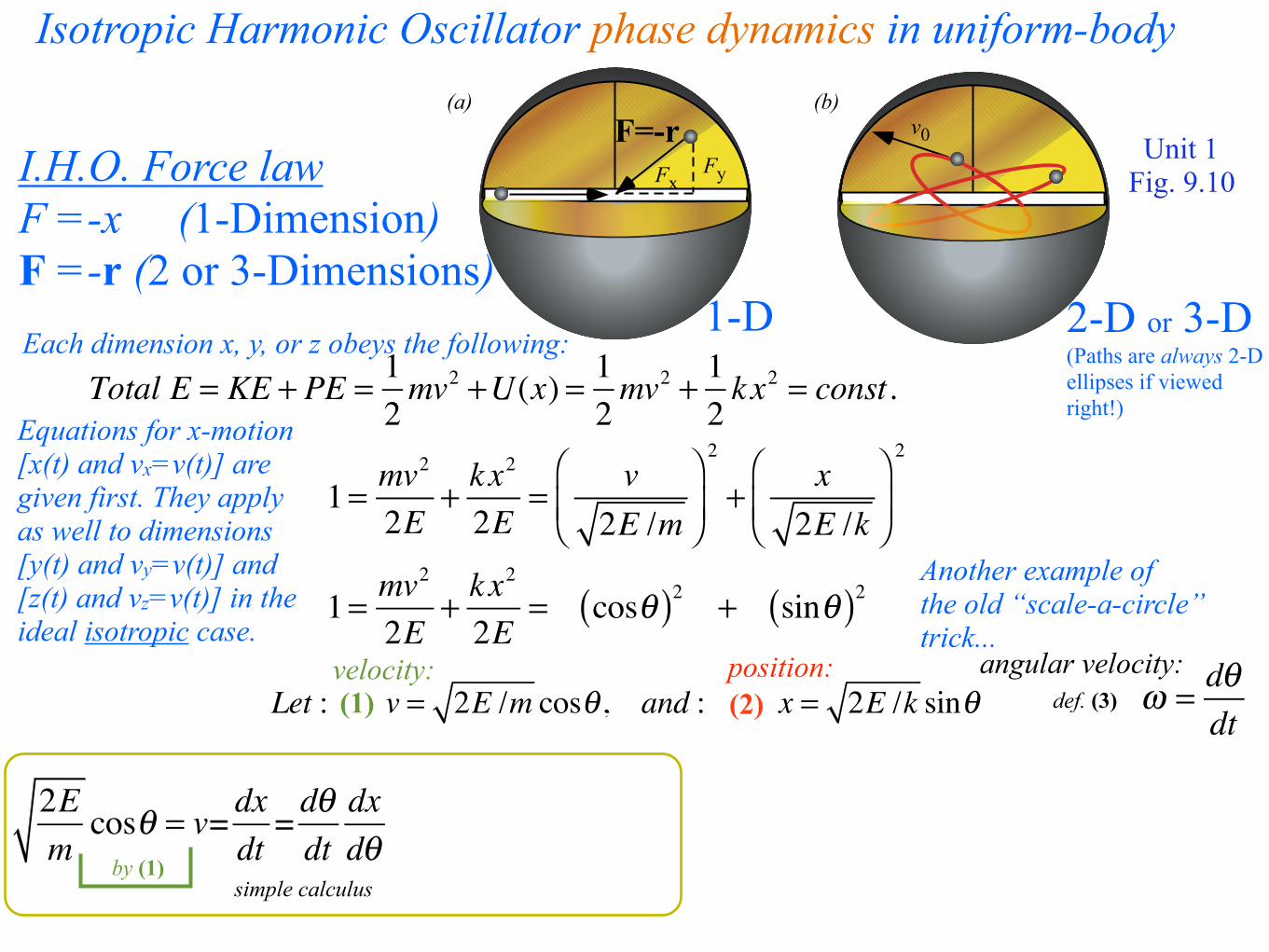
Isotropic Harmonic Oscillator phase dynamics in uniform-body

I.H.O. Force law F =-x (1-Dimension) F =-r (2 or 3-Dimensions)Each dimension x, y, or z obeys the following:

1-D 2-D or 3-D (Paths are always 2-D ellipses if viewed right!)

Unit 1 Fig. 9.10

Equations for x-motion [x(t) and vx=v(t)] are given first. They apply as well to dimensions [y(t) and vy=v(t)] and [z(t) and vz=v(t)] in the ideal isotropic case.

Total E = KE + PE = 12mv2 +U(x) = 1

2mv2 + 1

2kx2 = const.

Fx

v0Fy

F=-r(a) (b)

Total E = KE + PE = 12mv2 +U(x) = 1

2mv2 + 1

2kx2 = const.

1= mv2

2E+ kx

2

2E= v

2E /m⎛

⎝⎜⎞

⎠⎟

2

+ x2E /k

⎛

⎝⎜⎞

⎠⎟

2

1= mv2

2E+ kx

2

2E= cosθ( )2 + sinθ( )2

Let : v = 2E /m cosθ , and : x = 2E /k sinθ(1) (2)

Isotropic Harmonic Oscillator phase dynamics in uniform-body

I.H.O. Force law F =-x (1-Dimension) F =-r (2 or 3-Dimensions)Each dimension x, y, or z obeys the following:

Another example of the old “scale-a-circle” trick...

1-D

Unit 1 Fig. 9.10

Equations for x-motion [x(t) and vx=v(t)] are given first. They apply as well to dimensions [y(t) and vy=v(t)] and [z(t) and vz=v(t)] in the ideal isotropic case.

2-D or 3-D (Paths are always 2-D ellipses if viewed right!)

velocity: position:

Fx

v0Fy

F=-r(a) (b)

Total E = KE + PE = 12mv2 +U(x) = 1

2mv2 + 1

2kx2 = const.

1= mv2

2E+ kx

2

2E= v

2E /m⎛

⎝⎜⎞

⎠⎟

2

+ x2E /k

⎛

⎝⎜⎞

⎠⎟

2

1= mv2

2E+ kx

2

2E= cosθ( )2 + sinθ( )2

Let : v = 2E /m cosθ , and : x = 2E /k sinθ(1) (2)

Isotropic Harmonic Oscillator phase dynamics in uniform-body

I.H.O. Force law F =-x (1-Dimension) F =-r (2 or 3-Dimensions)Each dimension x, y, or z obeys the following:

Another example of the old “scale-a-circle” trick...

1-D

Unit 1 Fig. 9.10

Equations for x-motion [x(t) and vx=v(t)] are given first. They apply as well to dimensions [y(t) and vy=v(t)] and [z(t) and vz=v(t)] in the ideal isotropic case.

2-D or 3-D (Paths are always 2-D ellipses if viewed right!)

ω = dθdt

def. (3)velocity: position: angular velocity:

Fx

v0Fy

F=-r(a) (b)

Total E = KE + PE = 12mv2 +U(x) = 1

2mv2 + 1

2kx2 = const.

1= mv2

2E+ kx

2

2E= v

2E /m⎛

⎝⎜⎞

⎠⎟

2

+ x2E /k

⎛

⎝⎜⎞

⎠⎟

2

1= mv2

2E+ kx

2

2E= cosθ( )2 + sinθ( )2

2Emcosθ = v= dx

dt

Let : v = 2E /m cosθ , and : x = 2E /k sinθ(1) (2)

by (1)

Isotropic Harmonic Oscillator phase dynamics in uniform-body

I.H.O. Force law F =-x (1-Dimension) F =-r (2 or 3-Dimensions)Each dimension x, y, or z obeys the following:

Another example of the old “scale-a-circle” trick...

1-D

Unit 1 Fig. 9.10

Equations for x-motion [x(t) and vx=v(t)] are given first. They apply as well to dimensions [y(t) and vy=v(t)] and [z(t) and vz=v(t)] in the ideal isotropic case.

2-D or 3-D (Paths are always 2-D ellipses if viewed right!)

ω = dθdt

def. (3)velocity: position: angular velocity:

Fx

v0Fy

F=-r(a) (b)

Total E = KE + PE = 12mv2 +U(x) = 1

2mv2 + 1

2kx2 = const.

1= mv2

2E+ kx

2

2E= v

2E /m⎛

⎝⎜⎞

⎠⎟

2

+ x2E /k

⎛

⎝⎜⎞

⎠⎟

2

1= mv2

2E+ kx

2

2E= cosθ( )2 + sinθ( )2

2Emcosθ = v= dx

dt= dθdt

dxdθ

Let : v = 2E /m cosθ , and : x = 2E /k sinθ(1) (2)

by (1)

Isotropic Harmonic Oscillator phase dynamics in uniform-body

I.H.O. Force law F =-x (1-Dimension) F =-r (2 or 3-Dimensions)Each dimension x, y, or z obeys the following:

Another example of the old “scale-a-circle” trick...

1-D

Unit 1 Fig. 9.10

Equations for x-motion [x(t) and vx=v(t)] are given first. They apply as well to dimensions [y(t) and vy=v(t)] and [z(t) and vz=v(t)] in the ideal isotropic case.

2-D or 3-D (Paths are always 2-D ellipses if viewed right!)

ω = dθdt

def. (3)velocity: position: angular velocity:

simple calculus

Fx

v0Fy

F=-r(a) (b)

Total E = KE + PE = 12mv2 +U(x) = 1

2mv2 + 1

2kx2 = const.

1= mv2

2E+ kx

2

2E= v

2E /m⎛

⎝⎜⎞

⎠⎟

2

+ x2E /k

⎛

⎝⎜⎞

⎠⎟

2

1= mv2

2E+ kx

2

2E= cosθ( )2 + sinθ( )2

2Emcosθ = v= dx

dt= dθdt

dxdθ=ω dx

dθ

Let : v = 2E /m cosθ , and : x = 2E /k sinθ(1) (2)

by (1)by def. (3)

Isotropic Harmonic Oscillator phase dynamics in uniform-body

I.H.O. Force law F =-x (1-Dimension) F =-r (2 or 3-Dimensions)Each dimension x, y, or z obeys the following:

Another example of the old “scale-a-circle” trick...

1-D

Unit 1 Fig. 9.10

Equations for x-motion [x(t) and vx=v(t)] are given first. They apply as well to dimensions [y(t) and vy=v(t)] and [z(t) and vz=v(t)] in the ideal isotropic case.

2-D or 3-D (Paths are always 2-D ellipses if viewed right!)

ω = dθdt

def. (3)velocity: position: angular velocity:

Fx

v0Fy

F=-r(a) (b)

Total E = KE + PE = 12mv2 +U(x) = 1

2mv2 + 1

2kx2 = const.

1= mv2

2E+ kx

2

2E= v

2E /m⎛

⎝⎜⎞

⎠⎟

2

+ x2E /k

⎛

⎝⎜⎞

⎠⎟

2

1= mv2

2E+ kx

2

2E= cosθ( )2 + sinθ( )2

2Emcosθ = v= dx

dt= dθdt

dxdθ=ω dx

dθ=ω 2E

kcosθ

Let : v = 2E /m cosθ , and : x = 2E /k sinθ(1) (2)

by (1)by def. (3) by (2)

Isotropic Harmonic Oscillator phase dynamics in uniform-body

I.H.O. Force law F =-x (1-Dimension) F =-r (2 or 3-Dimensions)Each dimension x, y, or z obeys the following:

Another example of the old “scale-a-circle” trick...

1-D

Unit 1 Fig. 9.10

Equations for x-motion [x(t) and vx=v(t)] are given first. They apply as well to dimensions [y(t) and vy=v(t)] and [z(t) and vz=v(t)] in the ideal isotropic case.

2-D or 3-D (Paths are always 2-D ellipses if viewed right!)

ω = dθdt

def. (3)velocity: position: angular velocity:

Fx

v0Fy

F=-r(a) (b)

Total E = KE + PE = 12mv2 +U(x) = 1

2mv2 + 1

2kx2 = const.

1= mv2

2E+ kx

2

2E= v

2E /m⎛

⎝⎜⎞

⎠⎟

2

+ x2E /k

⎛

⎝⎜⎞

⎠⎟

2

1= mv2

2E+ kx

2

2E= cosθ( )2 + sinθ( )2

2Emcosθ = v= dx

dt= dθdt

dxdθ=ω dx

dθ=ω 2E

kcosθ ω = dθ

dt

Let : v = 2E /m cosθ , and : x = 2E /k sinθ(1) (2)

by (1)by def. (3) by (2)

by def. (3)

Isotropic Harmonic Oscillator phase dynamics in uniform-body

I.H.O. Force law F =-x (1-Dimension) F =-r (2 or 3-Dimensions)Each dimension x, y, or z obeys the following:

Another example of the old “scale-a-circle” trick...

1-D

Unit 1 Fig. 9.10

Equations for x-motion [x(t) and vx=v(t)] are given first. They apply as well to dimensions [y(t) and vy=v(t)] and [z(t) and vz=v(t)] in the ideal isotropic case.

2-D or 3-D (Paths are always 2-D ellipses if viewed right!)

ω = dθdt

def. (3)

Fx

v0Fy

F=-r(a) (b)

Total E = KE + PE = 12mv2 +U(x) = 1

2mv2 + 1

2kx2 = const.

1= mv2

2E+ kx

2

2E= v

2E /m⎛

⎝⎜⎞

⎠⎟

2

+ x2E /k

⎛

⎝⎜⎞

⎠⎟

2

1= mv2

2E+ kx

2

2E= cosθ( )2 + sinθ( )2

2Emcosθ = v= dx

dt= dθdt

dxdθ=ω dx

dθ=ω 2E

kcosθ ω = dθ

dt=

2Emcosθ

2Ekcosθ

Let : v = 2E /m cosθ , and : x = 2E /k sinθ(1) (2)

by (1)by def. (3) by (2)

by def. (3)

Isotropic Harmonic Oscillator phase dynamics in uniform-body

I.H.O. Force law F =-x (1-Dimension) F =-r (2 or 3-Dimensions)Each dimension x, y, or z obeys the following:

Another example of the old “scale-a-circle” trick...

1-D

Unit 1 Fig. 9.10

Equations for x-motion [x(t) and vx=v(t)] are given first. They apply as well to dimensions [y(t) and vy=v(t)] and [z(t) and vz=v(t)] in the ideal isotropic case.

2-D or 3-D (Paths are always 2-D ellipses if viewed right!)

ω = dθdt

def. (3)

by (2) derivative

divide (1)

Fx

v0Fy

F=-r(a) (b)

Total E = KE + PE = 12mv2 +U(x) = 1

2mv2 + 1

2kx2 = const.

1= mv2

2E+ kx

2

2E= v

2E /m⎛

⎝⎜⎞

⎠⎟

2

+ x2E /k

⎛

⎝⎜⎞

⎠⎟

2

1= mv2

2E+ kx

2

2E= cosθ( )2 + sinθ( )2

2Emcosθ = v= dx

dt= dθdt

dxdθ=ω dx

dθ=ω 2E

kcosθ ω = dθ

dt=

2Emcosθ

2Ekcosθ

= km

Let : v = 2E /m cosθ , and : x = 2E /k sinθ(1) (2)

by (1)by def. (3) by (2)

by def. (3)

Isotropic Harmonic Oscillator phase dynamics in uniform-body

I.H.O. Force law F =-x (1-Dimension) F =-r (2 or 3-Dimensions)Each dimension x, y, or z obeys the following:

Another example of the old “scale-a-circle” trick...

1-D

Unit 1 Fig. 9.10

Equations for x-motion [x(t) and vx=v(t)] are given first. They apply as well to dimensions [y(t) and vy=v(t)] and [z(t) and vz=v(t)] in the ideal isotropic case.

2-D or 3-D (Paths are always 2-D ellipses if viewed right!)

ω = dθdt

def. (3)

by (2) derivative

divide (1)

Fx

v0Fy

F=-r(a) (b)

Total E = KE + PE = 12mv2 +U(x) = 1

2mv2 + 1

2kx2 = const.

1= mv2

2E+ kx

2

2E= v

2E /m⎛

⎝⎜⎞

⎠⎟

2

+ x2E /k

⎛

⎝⎜⎞

⎠⎟

2

1= mv2

2E+ kx

2

2E= cosθ( )2 + sinθ( )2

2Emcosθ = v= dx

dt= dθdt

dxdθ=ω dx

dθ=ω 2E

kcosθ ω = dθ

dt= k

m

Let : v = 2E /m cosθ , and : x = 2E /k sinθ(1) (2)

by (1)by def. (3) by (2)

by def. (3)

Isotropic Harmonic Oscillator phase dynamics in uniform-body

I.H.O. Force law F =-x (1-Dimension) F =-r (2 or 3-Dimensions)Each dimension x, y, or z obeys the following:

Another example of the old “scale-a-circle” trick...

1-D

Unit 1 Fig. 9.10

Equations for x-motion [x(t) and vx=v(t)] are given first. They apply as well to dimensions [y(t) and vy=v(t)] and [z(t) and vz=v(t)] in the ideal isotropic case.

by integration given constant ω:

θ = ω⋅dt∫ =ω⋅t +α

2-D or 3-D (Paths are always 2-D ellipses if viewed right!)

ω = dθdt

def. (3)angular velocity:

Review of IHO orbital phasor “clock” dynamics in uniform-body with two “movie” examples

0 12

3

4

5

6

78-7-6

-5

-4

-3

-2-1

01

2

3 4 5

6

78

-7-6

-5

-4-3

-2-1

(2,4)(3,5)(4,6)

(5,7)

(6,8)

(7,-7)

x-position

x-velocity vx/ω

position

x

velocity vx/ω

(a) 1-D Oscillator Phasor Plot

(b) 2-D Oscillator Phasor Plot

Phasor goes

clockwise

by angle ω t

ω t

(8,-6)(9,-5)

y-velocity

vy/ω

(x-Phase 45°

behind

the y-Phase)y-position

φ counter-clockwise

if y is behind x

clockwise

orbit

if x is behind y

(1,3) Left-

handed

Right-

handed

(0,2)

Fx

v0Fy

F=-r(a) (b)

Unit 1 Fig. 9.10

Review of IHO orbital phase dynamics in uniform-body

Introduction to Phasors at our Pirelli Relativity SiteBoxIt web simulation - With y-Phasor is on other side of xy plot

RelaWavity web simulation - Contact ellipsometry

Geometry of Kepler anomalies for vectors [r(φ), v(φ)] in coordinate (x,y) space rendered by animation web-apps BoxIt and RelaWavity described below after p.70.RelaWavity web simulation - Contact ellipsometry (User Mouse Input allowed for setting phasor values)

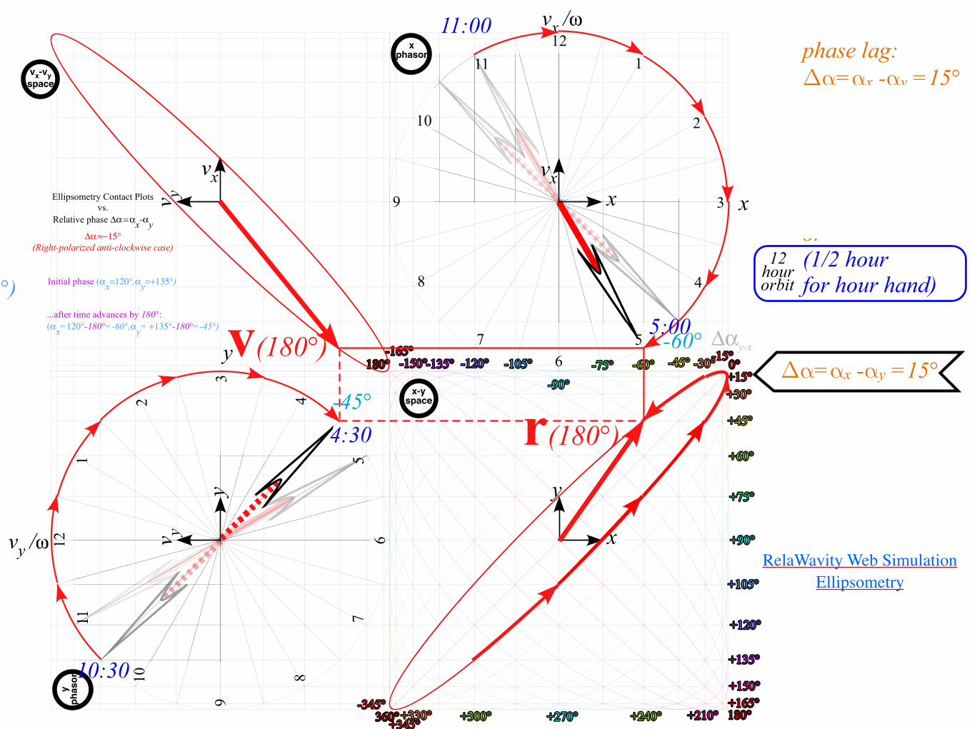
RelaWavity Web Simulation Ellipsometry

Geometry of Kepler anomalies for vectors [r(φ), v(φ)] in coordinate (x,y) space rendered by animation web-apps BoxIt and RelaWavity described below after p.7 and p.17.

RelaWavity web simulation - Contact ellipsometry (User Mouse Input allowed for setting phasor values)

RelaWavity Web Simulation Ellipsometry

x

y

121

2

3

4

56

7

8

9

10

121

2

3

4

56

7

8

9

10

11

00°°--1155°°--3300°°--4455°°++1155°°++3300°°

++4455°°

--6600°°

++6600°°

--7755°°

++7755°°

--9900°°

++9900°°

--110055°°

++110055°°

--112200°°

++112200°°

--113355°°

++113355°°

--115500°°

++115500°°

--116655°°

++116655°°

118800°°

118800°°++227700°° ++224400°°++330000°°336600°° ++221100°°++333300°°

vx /ω

vy /ω

Δαy-x

xphasor

yphasor

x-yspace

x

y

xvx

y

v y

++334455°°--334455°°

...after time advances by 180°:(αx=120°-180°=-60°,αy= +135°-180°=-45°)

r(180°)

Ellipsometry Contact Plotsvs.

Relative phase Δα=αx-αyΔα=−15°

(Right-polarized anti-clockwise case)

...after time advances by 180°:(αx=120°-180°=-60°,αy= +135°-180°=-45°)

Initial phase (αx=120°,αy=+135°)

vxv y

vx-vyspace

v(180°)-45°

-60°

phase lag: Δα=αx -αy =15° (2.5 seconds for second hand) or (2.5 minutes for minute hand) or (1/2 hour for hour hand)

1 minute orbit

1 hour orbit

12 hour orbit

Δα=αx -αy =15°

10:30

11:00

5:00

4:30

RelaWavity Web Simulation Ellipsometry

Constructing 2D IHO orbits using Kepler anomaly plots Mean-anomaly and eccentric-anomaly geometry Calculus and vector geometry of IHO orbits A confusing introduction to Coriolis-centrifugal force geometry (Derived better in Ch. 12)

b bsin ω t

ω t

ω ta cos ω t

ay=bsin ω t

x=a cos ω t

ω t

r

φ

b

-b

-b

a

a

-a

ω t

a

y=bsin ω t

x=a cos ω t

r

b

-b

-b

a

a

-a

-a

ω t

Step 1. Draw concentriccircles of radius a and band a radius OA at angleω t

Step 3. Draw horizontial line BRfrom b-circle at ω t to line AX.Intersection is orbit point R.

Step 2. Draw vertical line AXfrom a-circle at ωt to x-axis

O

A

O

A

O

A

X X

BR

abω t

b

-b

-b

a

-a

-a

ab

O X O X

Step 4-NRepeatas oftenas needed

ba

Linear HarmonicForce-FieldOrbits

Unit 1 Fig. 11.1

(top 2/3’s)

Kepler’s Mean Anomaly Line (slope angle θ =ωt)

Kepler’s Eccentric Anomaly Line

(slope is polar angle φ=atan[y/x])

A

RB

Zig!

Zag!

Another example of a

Zig-Zag construction:

b bsin ω t

ω t

ω ta cos ω t

ay=bsin ω t

x=a cos ω t

ω t

r

φ

b

-b

-b

a

a

-a

ω t

a

y=bsin ω t

x=a cos ω t

r

b

-b

-b

a

a

-a

-a

ω t

Step 1. Draw concentriccircles of radius a and band a radius OA at angleω t

Step 3. Draw horizontial line BRfrom b-circle at ω t to line AX.Intersection is orbit point R.

Step 2. Draw vertical line AXfrom a-circle at ωt to x-axis

O

A

O

A

O

A

X X

BR

abω t

b

-b

-b

a

-a

-a

ab

O X O X

Step 4-NRepeatas oftenas needed

ba

Linear HarmonicForce-FieldOrbits

Unit 1 Fig. 11.1

Kepler’s Mean Anomaly

Line

Kepler’s Eccentric Anomaly Line

(slope is polar angle φ=atan[y/x])

Constructing 2D IHO orbits using Kepler anomaly plots Mean-anomaly and eccentric-anomaly geometry Calculus and vector geometry of IHO orbits A confusing introduction to Coriolis-centrifugal force geometry (Derived better in Ch. 12)

r(t) φv(t)/ω

90°

a(t)/ω2

j(t)/ω3

acceleration

jerk

velocity

position

90°

r(t)φ=ω tv(t)/ω

a(t)/ω2

j(t)/ω3

acceleration

jerk

velocity

position

90°

90°

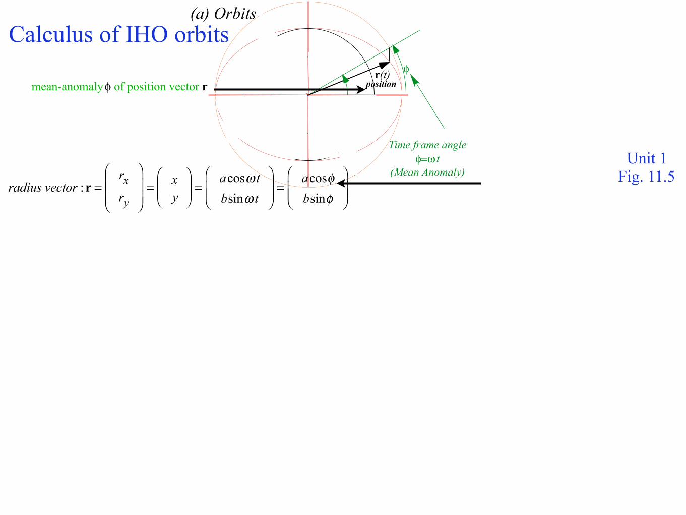
Time frame angle

φ=ω t(Mean Anomaly)

(a) Orbits (b) Tangents

radius vector :r =rx

ry

⎛

⎝⎜⎜

⎞

⎠⎟⎟= x

y

⎛

⎝⎜

⎞

⎠⎟ =

acosω tbsinω t

⎛

⎝⎜⎜

⎞

⎠⎟⎟=

acosφbsinφ

⎛

⎝⎜⎜

⎞

⎠⎟⎟

Unit 1 Fig. 11.5

Calculus of IHO orbits

mean-anomaly φ of position vector r

r(t) φv(t)/ω

90°

a(t)/ω2

j(t)/ω3

acceleration

jerk

velocity

position

90°

r(t)φ=ω tv(t)/ω

a(t)/ω2

j(t)/ω3

acceleration

jerk

velocity

position

90°

90°

Time frame angle

φ=ω t(Mean Anomaly)

(a) Orbits (b) Tangents

radius vector :r =rx

ry

⎛

⎝⎜⎜

⎞

⎠⎟⎟= x

y

⎛

⎝⎜

⎞

⎠⎟ =

acosω tbsinω t

⎛

⎝⎜⎜

⎞

⎠⎟⎟=

acosφbsinφ

⎛

⎝⎜⎜

⎞

⎠⎟⎟

velocity vector : v =vx

vy

⎛

⎝⎜⎜

⎞

⎠⎟⎟=

−aω sinω tbω cosω t

⎛

⎝⎜⎜

⎞

⎠⎟⎟= dr

dt= !r =

acos φ + 2π( )

bsin φ + 2π( )

⎛

⎝

⎜⎜⎜

⎞

⎠

⎟⎟⎟

( for ω = 1)

Unit 1 Fig. 11.5

Calculus of IHO orbitsTo make velocity vector v just rotate by π/2 or 90° the mean-anomaly φ of position vector r

mean-anomaly φ of position vector r rotated by π/2 or 90° is m.a. of vector v

r(t) φv(t)/ω

90°

a(t)/ω2

j(t)/ω3

acceleration

jerk

velocity

position

90°

r(t)φ=ω tv(t)/ω

a(t)/ω2

j(t)/ω3

acceleration

jerk

velocity

position

90°

90°

Time frame angle

φ=ω t(Mean Anomaly)

(a) Orbits (b) Tangents

radius vector :r =rx

ry

⎛

⎝⎜⎜

⎞

⎠⎟⎟= x

y

⎛

⎝⎜

⎞

⎠⎟ =

acosω tbsinω t

⎛

⎝⎜⎜

⎞

⎠⎟⎟=

acosφbsinφ

⎛

⎝⎜⎜

⎞

⎠⎟⎟

velocity vector : v =vx

vy

⎛

⎝⎜⎜

⎞

⎠⎟⎟=

−aω sinω tbω cosω t

⎛

⎝⎜⎜

⎞

⎠⎟⎟= dr

dt= !r =

acos φ + 2π( )

bsin φ + 2π( )

⎛

⎝

⎜⎜⎜

⎞

⎠

⎟⎟⎟

( for ω = 1)

accelerationor force vector :Fm= a =

ax

ay

⎛

⎝⎜⎜

⎞

⎠⎟⎟=

−aω 2 cosω t

−bω 2 sinω t

⎛

⎝⎜⎜

⎞

⎠⎟⎟= dv

dt= !v = !!r = d2r

dt2=

acos φ + 22π( )

bsin φ + 22π( )

⎛

⎝

⎜⎜⎜

⎞

⎠

⎟⎟⎟

Unit 1 Fig. 11.5

or changeof velocity

Calculus of IHO orbitsTo make velocity vector v just rotate by π/2 or 90° the mean-anomaly φ of position vector r

mean-anomaly φ of position vector r rotated by π/2 or 90° is m.a. of vector v

m.a. φ+π/2 of vector v rotated by another π/2 is m.a. of vector a

r(t) φv(t)/ω

90°

a(t)/ω2

j(t)/ω3

acceleration

jerk

velocity

position

90°

r(t)φ=ω tv(t)/ω

a(t)/ω2

j(t)/ω3

acceleration

jerk

velocity

position

90°

90°

Time frame angle

φ=ω t(Mean Anomaly)

(a) Orbits (b) Tangents

radius vector :r =rx

ry

⎛

⎝⎜⎜

⎞

⎠⎟⎟= x

y

⎛

⎝⎜

⎞

⎠⎟ =

acosω tbsinω t

⎛

⎝⎜⎜

⎞

⎠⎟⎟=

acosφbsinφ

⎛

⎝⎜⎜

⎞

⎠⎟⎟

velocity vector : v =vx

vy

⎛

⎝⎜⎜

⎞

⎠⎟⎟=

−aω sinω tbω cosω t

⎛

⎝⎜⎜

⎞

⎠⎟⎟= dr

dt= !r =

acos φ + 2π( )

bsin φ + 2π( )

⎛

⎝

⎜⎜⎜

⎞

⎠

⎟⎟⎟

( for ω = 1)

accelerationor force vector :Fm= a =

ax

ay

⎛

⎝⎜⎜

⎞

⎠⎟⎟=

−aω 2 cosω t

−bω 2 sinω t

⎛

⎝⎜⎜

⎞

⎠⎟⎟= dv

dt= !v = !!r = d2r

dt2=

acos φ + 22π( )

bsin φ + 22π( )

⎛

⎝

⎜⎜⎜

⎞

⎠

⎟⎟⎟

jerk or changeof acceleration : j=jxjy

⎛

⎝⎜⎜

⎞

⎠⎟⎟=

+aω 3sinω t

−bω 3cosω t

⎛

⎝⎜⎜

⎞

⎠⎟⎟= da

dt= !a = !!v = !!!r = d3r

dt3=

acos φ + 23π( )

bsin φ + 23π( )

⎛

⎝

⎜⎜⎜

⎞

⎠

⎟⎟⎟

Unit 1 Fig. 11.5

or changeof velocity or changeof velocity

Calculus of IHO orbitsTo make velocity vector v just rotate by π/2 or 90° the mean-anomaly φ of position vector r

mean-anomaly φ of position vector r rotated by π/2 or 90° is m.a. of vector v

m.a. φ+π/2 of vector v rotated by another π/2 is m.a. of vector a

...and so forth...

r(t) φv(t)/ω

90°

a(t)/ω2

j(t)/ω3

acceleration

jerk

velocity

position

90°

r(t)φ=ω tv(t)/ω

a(t)/ω2

j(t)/ω3

acceleration

jerk

velocity

position

90°

90°

Time frame angle

φ=ω t(Mean Anomaly)

(a) Orbits (b) Tangents

radius vector :r =rx

ry

⎛

⎝⎜⎜

⎞

⎠⎟⎟= x

y

⎛

⎝⎜

⎞

⎠⎟ =

acosω tbsinω t

⎛

⎝⎜⎜

⎞

⎠⎟⎟=

acosφbsinφ

⎛

⎝⎜⎜

⎞

⎠⎟⎟

velocity vector : v =vx

vy

⎛

⎝⎜⎜

⎞

⎠⎟⎟=

−aω sinω tbω cosω t

⎛

⎝⎜⎜

⎞

⎠⎟⎟= dr

dt= !r =

acos φ + 2π( )

bsin φ + 2π( )

⎛

⎝

⎜⎜⎜

⎞

⎠

⎟⎟⎟

( for ω = 1)

accelerationor force vector :Fm= a =

ax

ay

⎛

⎝⎜⎜

⎞

⎠⎟⎟=

−aω 2 cosω t

−bω 2 sinω t

⎛

⎝⎜⎜

⎞

⎠⎟⎟= dv

dt= !v = !!r = d2r

dt2=

acos φ + 22π( )

bsin φ + 22π( )

⎛

⎝

⎜⎜⎜

⎞

⎠

⎟⎟⎟

jerk or changeof acceleration : j=jxjy

⎛

⎝⎜⎜

⎞

⎠⎟⎟=

+aω 3sinω t

−bω 3cosω t

⎛

⎝⎜⎜

⎞

⎠⎟⎟= da

dt= !a = !!v = !!!r = d3r

dt3=

acos φ + 23π( )

bsin φ + 23π( )

⎛

⎝

⎜⎜⎜

⎞

⎠

⎟⎟⎟

inaugurationor changeof jerk :i =ixiy

⎛

⎝⎜⎜

⎞

⎠⎟⎟=

+aω 4 cosω t

+bω 4 sinω t

⎛

⎝⎜⎜

⎞

⎠⎟⎟= dj

dt= !j= !!a = !!!v = !!!!r = d4r

dt4=

acos φ + 24π( )

bsin φ + 24π( )

⎛

⎝

⎜⎜⎜

⎞

⎠

⎟⎟⎟

Unit 1 Fig. 11.5

or changeof velocity or changeof velocity or changeof velocity

Calculus of IHO orbitsTo make velocity vector v just rotate by π/2 or 90° the mean-anomaly φ of position vector r

mean-anomaly φ of position vector r rotated by π/2 or 90° is m.a. of vector v

m.a. φ+π/2 of vector v rotated by another π/2 is m.a. of vector a

...and so forth...

...and so on......But, now it repeats after 4 t-derivatives

r(t) φv(t)/ω

90°

a(t)/ω2

j(t)/ω3

acceleration

jerk

velocity

position

90°

r(t)φ=ω tv(t)/ω

a(t)/ω2

j(t)/ω3

acceleration

jerk

velocity

position

90°

90°

Time frame angle

φ=ω t(Mean Anomaly)

(a) Orbits (b) Tangents

radius vector :r =rx

ry

⎛

⎝⎜⎜

⎞

⎠⎟⎟= x

y

⎛

⎝⎜

⎞

⎠⎟ =

acosω tbsinω t

⎛

⎝⎜⎜

⎞

⎠⎟⎟=

acosφbsinφ

⎛

⎝⎜⎜

⎞

⎠⎟⎟

velocity vector : v =vx

vy

⎛

⎝⎜⎜

⎞

⎠⎟⎟=

−aω sinω tbω cosω t

⎛

⎝⎜⎜

⎞

⎠⎟⎟= dr

dt= !r =

acos φ + 2π( )

bsin φ + 2π( )

⎛

⎝

⎜⎜⎜

⎞

⎠

⎟⎟⎟

( for ω = 1)

accelerationor force vector :Fm= a =

ax

ay

⎛

⎝⎜⎜

⎞

⎠⎟⎟=

−aω 2 cosω t

−bω 2 sinω t

⎛

⎝⎜⎜

⎞

⎠⎟⎟= dv

dt= !v = !!r = d2r

dt2=

acos φ + 22π( )

bsin φ + 22π( )

⎛

⎝

⎜⎜⎜

⎞

⎠

⎟⎟⎟

jerk or changeof acceleration : j=jxjy

⎛

⎝⎜⎜

⎞

⎠⎟⎟=

+aω 3sinω t

−bω 3cosω t

⎛

⎝⎜⎜

⎞

⎠⎟⎟= da

dt= !a = !!v = !!!r = d3r

dt3=

acos φ + 23π( )

bsin φ + 23π( )

⎛

⎝

⎜⎜⎜

⎞

⎠

⎟⎟⎟

inaugurationor changeof jerk :i =ixiy

⎛

⎝⎜⎜

⎞

⎠⎟⎟=

+aω 4 cosω t

+bω 4 sinω t

⎛

⎝⎜⎜

⎞

⎠⎟⎟= dj

dt= !j= !!a = !!!v = !!!!r = d4r

dt4=

acos φ + 24π( )

bsin φ + 24π( )

⎛

⎝

⎜⎜⎜

⎞

⎠

⎟⎟⎟

Unit 1 Fig. 11.5

or changeof velocity or changeof velocity or changeof velocity

Calculus of IHO orbitsTo make velocity vector v just rotate by π/2 or 90° the mean-anomaly φ of position vector r

mean-anomaly φ of position vector r rotated by π/2 or 90° is m.a. of vector v

m.a. φ+π/2 of vector v rotated by another π/2 is m.a. of vector a

...and so forth...

...and so on......But, now it repeats after 4 t-derivatives

Link → IHO Exegesis Plot

Link ⇒ BoxIt simulation of IHO orbits

Link → IHO orbital time rates of change

Geometry of Kepler anomalies for vectors [r(φ), v(φ), a(φ), j(φ),] in coordinate (x,y) space rendered by animation web-apps BoxIt and RelaWavity.

RelaWavity orbit web-app

Link → IHO orbital time rates of change

https://modphys.hosted.uark.edu/markup/BoxItWeb.html

Geometry of Kepler anomalies for vectors [r(φ)] in coordinate (x,y) space and 2-particle (x1,x2) space rendered by animation web-apps BoxIt.

BoxIt Web Stokes Simulation

BoxIt minimal detailBoxIt more detailBoxIt still more detail

Geometry of Kepler anomalies for vectors [r(φ), v(φ), a(φ), j(φ),] in coordinate (x,y) space and 2-particle (x1,x2) space rendered by animation web-apps BoxIt. BoxIt Web Simulation - w/Derivatives

BoxIt minimal detailBoxIt more detailBoxIt still more detail

Geometry of vectors [r(φ), p(φ)] and quantum spin S-space and 2-particle (x1,x2) space rendered by animation web-apps BoxIt.

BoxIt Web Simulation - B-Type Motion

BoxIt minimal detailBoxIt more detailBoxIt still more detail

Constructing 2D IHO orbits using Kepler anomaly plots Mean-anomaly and eccentric-anomaly geometry Calculus and vector geometry of IHO orbits A confusing introduction to Coriolis-centrifugal force geometry (Derived better in Ch. 12)

F = -kr

orbital velocity=V

(b) “Carnival kid” orbiting inspace attached to a spring

centrifugalforce=+kr=+mω2r

ω t

centripetalforce=

(due to spring)

Carnival kidsays:

“This is awful!I can hardlyhold ontothis darnspring.”

F = -kr

orbital velocity=V

(a) “Earthronaut” orbitingtunnel inside Earth

centrifugalforce=+kr=+mω2r

ω t

centripetalforce=

(due to gravity)

Earthronautsays:

“This is great!I’m weightless.”

apogee(x=a, y=0)aphelion=a

perigee(x=0,y=b)

θperhelion=bmass gaining speed

as it falls

VelocityV

θVelocityV centripetal force F=-kr

Negative power( F•V=|F||V|cos θ <0)

Positive power( F•V=|F||V|cos θ >0)

mass losing speedas it rises

Unit 1 Fig. 11.2

Unit 1 Fig. 11.3

(Radius r decreasing)(Radius r increasing)

centrifugal force

Velocityalongradialpath

Coriolis force(depends onradial pathspeed)

RotationalvelocityV=ωr

(a) Centrifugal and CoriolisForces on Merry-Go-Round

centrifugal force

Velocityalongradialpath

Coriolis forcePhysicist Force (where m wants to go)

Mathematician Force (to hold m back)

Constraint force keeps m in radial slot

centrifugal force

Velocityalongradialpath

Coriolis force(depends onradial pathspeed)

RotationalvelocityV=ωr

(a) Centrifugal and CoriolisForces on Merry-Go-Round

centrifugal force

Velocityalongradialpath

Coriolis forcePhysicist Force (where m wants to go)

Mathematician Force (to hold m back)

Constraint force keeps m in radial slot

Velocity

V

centripetal force F=-kr

centrifugal force

Total inertial force F=+kr

Coriolis forcecircle

of

curvature

(b) Centrifugal and Coriolis

Forces on Oscillator Orbit

(Falling phase)

centrifugal force

Velocityalongradialpath

Coriolis force(depends onradial pathspeed)

RotationalvelocityV=ωr

(a) Centrifugal and CoriolisForces on Merry-Go-Round

centrifugal force

Velocityalongradialpath

Coriolis forcePhysicist Force (where m wants to go)

Mathematician Force (to hold m back)

Constraint force keeps m in radial slot

Velocity

V

centripetal force F=-kr

centrifugal force

Total inertial force F=+kr

Coriolis forcecircle

of

curvature

(b) Centrifugal and Coriolis

Forces on Oscillator Orbit

(Falling phase)

centrifugal force

Velocityalongradialpath

Coriolis force(depends onradial pathspeed)

RotationalvelocityV=ωr

(a) Centrifugal and CoriolisForces on Merry-Go-Round

centrifugal force

Velocityalongradialpath

Coriolis forcePhysicist Force (where m wants to go)

Mathematician Force (to hold m back)

Constraint force keeps m in radial slot

(c) Centrifugal and Coriolis

Forces on Oscillator Orbit

(Rising phase)

Velocity

V

centripetal force F=-kr

centrifugal force

Total inertial force F=+kr

Coriolis force

circle

of

curvature

Velocity

V

centripetal force F=-kr

centrifugal force

Total inertial force F=+kr

Coriolis force

centrifugal force

Velocity

along

radial

path

Coriolis force

(depends on

radial path

speed)

Rotational

velocity

V=ωr

circle

of

curvature

Velocity

V

centrifugal force is

Total inertial force F=+kr

circle

of

curvature

(a) Centrifugal and Coriolis

Forces on Merry-Go-Round

(b) Centrifugal and Coriolis

Forces on Oscillator Orbit

(Falling phase)

(c) Centrifugal and Coriolis

Forces on Oscillator Orbit

(Rising phase)

centrifugal force

Velocity

along

radial

path

Coriolis force

centripetal force F=-kr

Velocity

V

centripetal force F=-kr

centrifugal force

Total inertial force F=+kr

Coriolis force

circle

of

curvature

(d) Centrifugal Force

on Oscillator Orbit

(apogee and perigee)

Velocity

V

centripetal force F=-kr

centrifugal force is

Total inertial force F=+kr

Unit 1 Fig. 11.4

a-d

A little confusing? Discussion of Coriolis forces will be done more elegantly and made more physically intuitive in Ch. 12 of Unit1 and in Unit 6.

Physicist Force (where m wants to go)

Mathematician Force (to hold m back)

Constraint force keeps m in radial slot

Some Kepler’s “laws” for all central (isotropic) force F(r) fields Angular momentum invariance of IHO: F(r)=-k·r with U(r)=k·r2/2 (Derived here) Angular momentum invariance of Coulomb: F(r)=-GMm/r2 with U(r)=-GMm·/r (Derived in Unit 5) Total energy E=KE+PE invariance of IHO: F(r)=-k·r (Derived here) Total energy E=KE+PE invariance of Coulomb: F(r)=-GMm/r2 (Derived in Unit 5)

1. Area of triangle ! rv = r × v/2 is constant

r × v = rxvy − ryvx = acosω t ⋅ bω cosω t( )− bsinω t ⋅ −aω sinω t( ) = ab ⋅ω cos2ω t + sin2ω t( )

t = 0 t = π/3ω t = π/2ωv=a ωv=b ω

r rr

ba

Unit 1 Fig. 11.8

Some Kepler’s “laws” for central (isotropic) force F(r) ...and certainly apply to the IHO: F(r)=-k·r with U(r)=k·r2/2

for IHO

vx

vy

⎛

⎝⎜⎜

⎞

⎠⎟⎟=

−aω sinω tbω cosω t

⎛

⎝⎜⎜

⎞

⎠⎟⎟

rxry

⎛

⎝⎜⎜

⎞

⎠⎟⎟= x

y

⎛

⎝⎜

⎞

⎠⎟ =

acosω tbsinω t

⎛

⎝⎜⎜

⎞

⎠⎟⎟

(Recall from Lecture 6: k = Gm 4π

3ρ⊕ )

1. Area of triangle ! rv = r × v/2 is constant

r × v = rxvy − ryvx = acosω t ⋅ bω cosω t( )− asinω t ⋅ −bω sinω t( ) = ab ⋅ω

2. Angular momentum L = mr × v is conserved

L = m |r × v |= m rxvy − ryvx( ) = m ⋅ab ⋅ω

t = 0 t = π/3ω t = π/2ωv=a ωv=b ω

r rr

ba

Unit 1 Fig. 11.8

Some Kepler’s “laws” that apply to any central (isotropic) force F(r) ...and certainly apply to the IHO: F(r)=-k·r with U(r)=k·r2/2

for IHO

for IHO

rv

|r×v| =r·v·sin!rv

(Recall from Lecture 6: k = Gm 4π

3ρ⊕ )

1. Area of triangle ! rv = r × v/2 is constant

r × v = rxvy − ryvx = acosω t ⋅ bω cosω t( )− asinω t ⋅ −bω sinω t( ) = ab ⋅ω2. Angular momentum L = mr × v is conserved

L = m |r × v |= m rxvy − ryvx( ) = m ⋅ab ⋅ω

t = 0 t = π/3ω t = π/2ωv=a ωv=b ω

r rr

ba

Unit 1 Fig. 11.8

Some Kepler’s “laws” that apply to any central (isotropic) force F(r) ...and certainly apply to the IHO: F(r)=-k·r with U(r)=k·r2/2

for IHO

for IHO

3. Equal area is swept by radius vector in each equal time interval T

AT =r × dr

20

T

∫ =r × dr

dt2

dt0

T

∫ = r × v2

dt0

T

∫ = L2m

dt0

T

∫ = L2m

T for IHO

by 2.

rdr

|r×dr| =r·dr·sin!rdr

(Recall from Lecture 6: k = Gm 4π

3ρ⊕ )

1. Area of triangle ! rv = r × v/2 is constant

r × v = rxvy − ryvx = acosω t ⋅ bω cosω t( )− asinω t ⋅ −bω sinω t( ) = ab ⋅ω2. Angular momentum L = mr × v is conserved

L = mr × v = m rxvy − ryvx( ) = m ⋅ab ⋅ω = m ⋅ab ⋅ 2πτ

t = 0 t = π/3ω t = π/2ωv=a ωv=b ω

r rr

ba

Unit 1 Fig. 11.8

Some Kepler’s “laws” that apply to any central (isotropic) force F(r) ...and certainly apply to the IHO: F(r)=-k·r with U(r)=k·r2/2

for IHO

for IHO

3. Equal area is swept by radius vector in each equal time interval T

AT =r × dr

20

T

∫ =r × dr

dt2

dt0

T

∫ = r × v2

dt0

T

∫ = L2m

dt0

T

∫ = L2m

T for IHO

In one period: τ= 1υ

= 2πω

= 2mAτ

L the area is: Aτ =

Lτ2m

( = ab ⋅π for ellipse orbit)

(Recall from Lecture 6: k = Gm 4π

3ρ⊕ )

1. Area of triangle ! rv = r × v/2 is constant

r × v = rxvy − ryvx = acosω t ⋅ bω cosω t( )− asinω t ⋅ −bω sinω t( ) = ab ⋅ω2. Angular momentum L = mr × v is conserved

L = mr × v = m rxvy − ryvx( ) = m ⋅ab ⋅ω = m ⋅ab ⋅ 2πτ

t = 0 t = π/3ω t = π/2ωv=a ωv=b ω

r rr

ba

Unit 1 Fig. 11.8

Some Kepler’s “laws” that apply to any central (isotropic) force F(r) ...and certainly apply to the IHO: F(r)=-k·r with U(r)=k·r2/2

for IHO

for IHO

3. Equal area is swept by radius vector in each equal time interval T

AT =r × dr

20

T

∫ =r × dr

dt2

dt0

T

∫ = r × v2

dt0

T

∫ = L2m

dt0

T

∫ = L2m

T for IHO

In one period: τ= 1υ

= 2πω

= 2mAτ

L the area is: Aτ =

Lτ2m

( = ab ⋅π for ellipse orbit)

( Recall from Lecture 6: ω = k /m = Gρ⊕4π / 3 )

(Recall from Lecture 6: k = Gm 4π

3ρ⊕ )

(IHO formulas from Lect. 6 p.70-79)

Some Kepler’s “laws” for all central (isotropic) force F(r) fields Angular momentum invariance of IHO: F(r)=-k·r with U(r)=k·r2/2 (Derived here) Angular momentum invariance of Coulomb: F(r)=-GMm/r2 with U(r)=-GMm·/r (Derived in Unit 5) Total energy E=KE+PE invariance of IHO: F(r)=-k·r (Derived here) Total energy E=KE+PE invariance of Coulomb: F(r)=-GMm/r2 (Derived in Unit 5)

1. Area of triangle ! rv = r × v/2 is constant

r × v = rxvy − ryvx =ab ⋅ Gρ⊕4π / 3 for IHO

a−1/2b GM⊕ for Coul.

⎧⎨⎪

⎩⎪

t = 0 t = π/3ω t = π/2ωv=a ωv=b ω

r rr

ba

Some Kepler’s “laws” that apply to any central (isotropic) force F(r) Apply to IHO: F(r)=-k·r with U(r)=k·r2/2 and Coulomb: F(r)=-GMm/r2 with U(r)=-GMm·/r

for IHO

t = 0 vv

r rrba

v

vrCoulomb:

IHO:

for Coul.(Derived in Unit 5)

(IHO formulas from Lect. 6 p.70-79)

1. Area of triangle ! rv = r × v/2 is constant

r × v = rxvy − ryvx =ab ⋅ Gρ⊕4π / 3 for IHO

a−1/2b GM⊕ for Coul.

⎧⎨⎪

⎩⎪2. Angular momentum L = mr × v is conserved

L = mr × v = m rxvy − ryvx( ) = m·ab ⋅ Gρ⊕4π / 3 for IHO

m·a−1/2b GM⊕ for Coul.

⎧⎨⎪

⎩⎪

t = 0 t = π/3ω t = π/2ωv=a ωv=b ω

r rr

ba

Some Kepler’s “laws” that apply to any central (isotropic) force F(r) Apply to IHO: F(r)=-k·r with U(r)=k·r2/2 and Coulomb: F(r)=-GMm/r2 with U(r)=-GMm·/r

for IHO

for IHO

t = 0 vv

r rrba

v

vrCoulomb:

IHO:

for Coul.

for Coul.

(Derived in Unit 5)

(... in Unit 5)

(IHO formulas from Lect. 6 p.70-79)

1. Area of triangle ! rv = r × v/2 is constant

r × v = rxvy − ryvx =ab ⋅ Gρ⊕4π / 3 for IHO

a−1/2b GM⊕ for Coul.

⎧⎨⎪

⎩⎪2. Angular momentum L = mr × v is conserved

L = mr × v = m rxvy − ryvx( ) = m·ab ⋅ Gρ⊕4π / 3 for IHO

m·a−1/2b GM⊕ for Coul.

⎧⎨⎪

⎩⎪

t = 0 t = π/3ω t = π/2ωv=a ωv=b ω

r rr

ba

Some Kepler’s “laws” that apply to any central (isotropic) force F(r) Apply to IHO: F(r)=-k·r with U(r)=k·r2/2 and Coulomb: F(r)=-GMm/r2 with U(r)=-GMm·/r

for IHO

for IHO

3. Equal area is swept by radius vector in each equal time interval T

τ= 1υ= 2πω

= 2mAτ

L= 2m·ab ⋅π

L=

2m·ab ⋅πm·ab ⋅ Gρ⊕4π / 3

2m·ab ⋅πm·a−1/2b GM⊕

⎧

⎨

⎪⎪

⎩

⎪⎪

t = 0 vv

r rrba

v

vrCoulomb:

IHO:

for Coul.

for Coul.

In one period:

Applies to any central

F(r)

Applies to IHO and Coulomb

(Derived in Unit 5)

(... in Unit 5)

(IHO formulas from Lect. 6 p.70-79)

1. Area of triangle ! rv = r × v/2 is constant

r × v = rxvy − ryvx =ab ⋅ Gρ⊕4π / 3 for IHO

a−1/2b GM⊕ for Coul.

⎧⎨⎪

⎩⎪2. Angular momentum L = mr × v is conserved

L = mr × v = m rxvy − ryvx( ) = m·ab ⋅ Gρ⊕4π / 3 for IHO

m·a−1/2b GM⊕ for Coul.

⎧⎨⎪

⎩⎪

t = 0 t = π/3ω t = π/2ωv=a ωv=b ω

r rr

ba

Some Kepler’s “laws” that apply to any central (isotropic) force F(r) Apply to IHO: F(r)=-k·r with U(r)=k·r2/2 and Coulomb: F(r)=-GMm/r2 with U(r)=-GMm·/r

for IHO

for IHO

3. Equal area is swept by radius vector in each equal time interval T

τ= 1υ= 2πω

= 2mAτ

L= 2m·ab ⋅π

L=

2m·ab ⋅πm·ab ⋅ Gρ⊕4π / 3

= 2πGρ⊕4π / 3

for IHO

2m·ab ⋅πm·a−1/2b GM⊕

= 2πa−3/2 GM⊕

for Coul.

⎧

⎨

⎪⎪

⎩

⎪⎪

t = 0 vv

r rrba

v

vrCoulomb:

IHO:

for Coul.

for Coul.

In one period:

that is ωIHO

that is ωCoul

Applies to any central

F(r)

Applies to IHO and Coulomb

(not a function of b)

(Derived in Unit 5)

(... in Unit 5)

(not a function of a or b)

Some Kepler’s “laws” for all central (isotropic) force F(r) fields Angular momentum invariance of IHO: F(r)=-k·r with U(r)=k·r2/2 (Derived here) Angular momentum invariance of Coulomb: F(r)=-GMm/r2 with U(r)=-GMm·/r (Derived in Unit 5) Total energy E=KE+PE invariance of IHO: F(r)=-k·r (Derived here) Total energy E=KE+PE invariance of Coulomb: F(r)=-GMm/r2 (Derived in Unit 5)

Kepler laws involve !-momentum conservation in isotropic force F(r) Now consider orbital energy conservation of the IHO: F(r)=-k·r with U(r)=k·r2/2

Total energy=KE+PE is constant

KE + PE = 12v iM i v + 1

2r iK i r

= 12

vx vy( )• m 00 m

⎛⎝⎜

⎞⎠⎟•

vxvy

⎛

⎝⎜⎜

⎞

⎠⎟⎟+ rx ry( )• k 0

0 k⎛⎝⎜

⎞⎠⎟•

rxry

⎛

⎝⎜⎜

⎞

⎠⎟⎟

= 12mv2

x + 12mv2

y + 12kr2

x + 12kr2

y

= 12m(−aω sinω t)2 + 1

2m(bω cosω t)2 + 1

2k(acosω t)2 + 1

2k(bsinω t)2

vx

vy

⎛

⎝⎜⎜

⎞

⎠⎟⎟=

−aω sinω tbω cosω t

⎛

⎝⎜⎜

⎞

⎠⎟⎟

rxry

⎛

⎝⎜⎜

⎞

⎠⎟⎟= x

y

⎛

⎝⎜

⎞

⎠⎟ =

acosω tbsinω t

⎛

⎝⎜⎜

⎞

⎠⎟⎟

Kepler laws involve !-momentum conservation in isotropic force F(r) Now consider orbital energy conservation of the IHO: F(r)=-k·r with U(r)=k·r2/2

Total IHO energy=KE+PE is constant

KE + PE = 12v iM i v + 1

2r iK i r

= 12

vx vy( )• m 00 m

⎛⎝⎜

⎞⎠⎟•

vxvy

⎛

⎝⎜⎜

⎞

⎠⎟⎟+ rx ry( )• k 0

0 k⎛⎝⎜

⎞⎠⎟•

rxry

⎛

⎝⎜⎜

⎞

⎠⎟⎟

= 12mv2

x + 12mv2

y + 12kr2

x + 12kr2

y

= 12m(−aω sinω t)2 + 1

2m(bω cosω t)2 + 1

2k(acosω t)2 + 1

2k(bsinω t)2

= 12ma2ω 2 (sin2ω t) + 1

2mb2ω 2 (cos2ω t)2 + 1

2ka2 (cos2ω t) + 1

2kb2 (sin2ω t)

= 12mω 2 (a2 + b2 ) Given : k = mω 2

= 12ma2ω 2 (sin2ω t) + 1

2mb2ω 2 (cos2ω t)2 + 1

2ka2 (cos2ω t) + 1

2kb2 (sin2ω t)

= 12mω 2 (a2 + b2 ) Given : k = mω 2

E = KE + PE = 12mω 2 (a2 + b2 ) = 1

2k(a2 + b2 ) since: ω = k

m = Gρ⊕4π / 3 or: mω 2 = k

Kepler laws involve !-momentum conservation in isotropic force F(r) Now consider orbital energy conservation of the IHO: F(r)=-k·r with U(r)=k·r2/2

Total IHO energy=KE+PE is constant

KE + PE = 12v iM i v + 1

2r iK i r

= 12

vx vy( )• m 00 m

⎛⎝⎜

⎞⎠⎟•

vxvy

⎛

⎝⎜⎜

⎞

⎠⎟⎟+ rx ry( )• k 0

0 k⎛⎝⎜

⎞⎠⎟•

rxry

⎛

⎝⎜⎜

⎞

⎠⎟⎟

= 12mv2

x + 12mv2

y + 12kr2

x + 12kr2

y

= 12m(−aω sinω t)2 + 1

2m(bω cosω t)2 + 1

2k(acosω t)2 + 1

2k(bsinω t)2

(IHO formulas from Lect. 6 p.70-79)

Some Kepler’s “laws” for all central (isotropic) force F(r) fields Angular momentum invariance of IHO: F(r)=-k·r with U(r)=k·r2/2 (Derived here) Angular momentum invariance of Coulomb: F(r)=-GMm/r2 with U(r)=-GMm·/r (Derived in Unit 5) Total energy E=KE+PE invariance of IHO: F(r)=-k·r (Derived here) Total energy E=KE+PE invariance of Coulomb: F(r)=-GMm/r2 (Derived in Unit 5)

Kepler laws involve !-momentum conservation in isotropic force F(r) Now consider orbital energy conservation of the IHO: F(r)=-k·r with U(r)=k·r2/2

We'll see that the Coul. orbits are simpler: (like the period...not a function of b)

Total IHO energy=KE+PE is constant

KE + PE = 12v iM i v + 1

2r iK i r

= 12

vx vy( )• m 00 m

⎛⎝⎜

⎞⎠⎟•

vxvy

⎛

⎝⎜⎜

⎞

⎠⎟⎟+ rx ry( )• k 0

0 k⎛⎝⎜

⎞⎠⎟•

rxry

⎛

⎝⎜⎜

⎞

⎠⎟⎟

= 12mv2

x + 12mv2

y + 12kr2

x + 12kr2

y

= 12m(−aω sinω t)2 + 1

2m(bω cosω t)2 + 1

2k(acosω t)2 + 1

2k(bsinω t)2

= 12ma2ω 2 (sin2ω t) + 1

2mb2ω 2 (cos2ω t)2 + 1

2ka2 (cos2ω t) + 1

2kb2 (sin2ω t)

= 12mω 2 (a2 + b2 ) Given : k = mω 2

E = KE + PE = 12mω 2 (a2 + b2 ) = 1

2k(a2 + b2 ) since: ω = k

m = Gρ⊕4π / 3 or: mω 2 = k

(IHO formulas from Lect. 6 p.70-79)

Kepler laws involve !-momentum conservation in isotropic force F(r) Now consider orbital energy conservation of the IHO: F(r)=-k·r with U(r)=k·r2/2

We'll see that the Coul. orbits are simpler: (like the period...not a function of b)

E = KE + PE = 12mv2

x +12mv2

y −kr= 1

2mv2

x +12mv2

y −GM⊕m

r= −GM⊕m

a

Total IHO energy=KE+PE is constant

KE + PE = 12v iM i v + 1

2r iK i r

= 12

vx vy( )• m 00 m

⎛⎝⎜

⎞⎠⎟•

vxvy

⎛

⎝⎜⎜

⎞

⎠⎟⎟+ rx ry( )• k 0

0 k⎛⎝⎜

⎞⎠⎟•

rxry

⎛

⎝⎜⎜

⎞

⎠⎟⎟

= 12mv2

x + 12mv2

y + 12kr2

x + 12kr2

y

= 12m(−aω sinω t)2 + 1

2m(bω cosω t)2 + 1

2k(acosω t)2 + 1

2k(bsinω t)2

= 12ma2ω 2 (sin2ω t) + 1

2mb2ω 2 (cos2ω t)2 + 1

2ka2 (cos2ω t) + 1

2kb2 (sin2ω t)

= 12mω 2 (a2 + b2 ) Given : k = mω 2

E = KE + PE = 12mω 2 (a2 + b2 ) = 1

2k(a2 + b2 ) since: ω = k

m = Gρ⊕4π / 3 or: mω 2 = k

Introduction to dual matrix operator contact geometry (based on IHO orbits) Quadratic form ellipse r•Q•r=1 vs.inverse form ellipse p•Q -1•p=1

Duality norm relations ( r•p=1) Q-Ellipse tangents r′ normal to dual Q -1-ellipse position p ( r′•p=0=r•p′)

Operator geometric sequences and eigenvectors Alternative scaling of matrix operator geometry

Vector calculus of tensor operation

Quadratic forms and tangent contact geometry of their ellipses

r •Q• r = 1

x y( )•1

a20

0 1

b2

⎛

⎝

⎜⎜⎜⎜⎜

⎞

⎠

⎟⎟⎟⎟⎟

• xy

⎛

⎝⎜

⎞

⎠⎟ = 1= x y( )•

x

a2

y

b2

⎛

⎝

⎜⎜⎜⎜⎜

⎞

⎠

⎟⎟⎟⎟⎟

= x2

a2+ y2

b2

A inverse matrix Q-1 generates an ellipse by p•Q -1•p=1 called inverse or dual ellipse:

p•Q−1•p = 1

px py( )• a2 0

0 b2

⎛

⎝⎜⎜

⎞

⎠⎟⎟•

px

py

⎛

⎝⎜⎜

⎞

⎠⎟⎟= 1= px py( )• a2 px

b2 py

⎛

⎝

⎜⎜⎜

⎞

⎠

⎟⎟⎟= a2 px

2 + b2 py2

Q• r

r

Q−1•p

p

A matrix Q that generates an ellipse by r•Q•r=1 is called positive-definite (if r•Q•r always >0)

Quadratic forms and tangent contact geometry of their ellipsesA matrix Q that generates an ellipse by r•Q•r=1 is called positive-definite (if r•Q•r always >0)

r •Q• r = 1

x y( )•1

a20

0 1

b2

⎛

⎝

⎜⎜⎜⎜⎜

⎞

⎠

⎟⎟⎟⎟⎟

• xy

⎛

⎝⎜

⎞

⎠⎟ = 1= x y( )•

x

a2

y

b2

⎛

⎝

⎜⎜⎜⎜⎜

⎞

⎠

⎟⎟⎟⎟⎟

= x2

a2+ y2

b2

A inverse matrix Q-1 generates an ellipse by p•Q -1•p=1 called inverse or dual ellipse:

p•Q−1•p = 1

px py( )• a2 0

0 b2

⎛

⎝⎜⎜

⎞

⎠⎟⎟•

px

py

⎛

⎝⎜⎜

⎞

⎠⎟⎟= 1= px py( )• a2 px

b2 py

⎛

⎝

⎜⎜⎜

⎞

⎠

⎟⎟⎟= a2 px

2 + b2 py2

Q• r = p

r

Q−1•p = r

p

Defined mapping between ellipses

Introduction to dual matrix operator contact geometry (based on IHO orbits) Quadratic form ellipse r•Q•r=1 vs.inverse form ellipse p•Q -1•p=1

Duality norm relations ( r•p=1) Q-Ellipse tangents r′ normal to dual Q -1-ellipse position p ( r′•p=0=r•p′)

Operator geometric sequences and eigenvectors Alternative scaling of matrix operator geometry

Vector calculus of tensor operation

r(φ)

φ=ω t

ab

b-circle

a-circle

Original ellipse

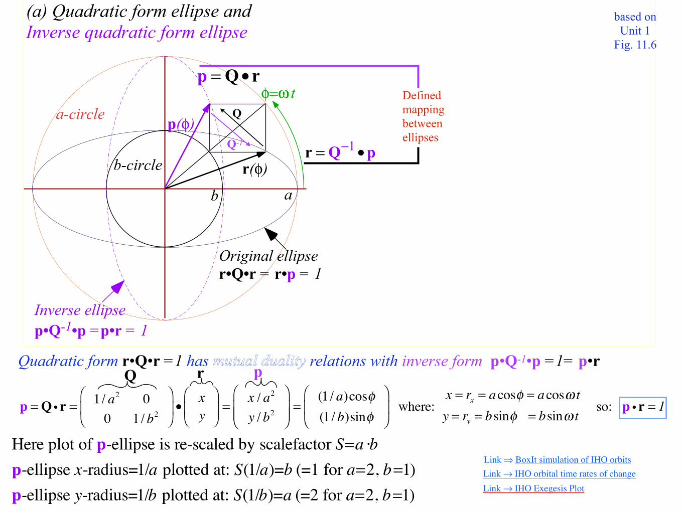
r•Q•r = r•p = 1

Inverse ellipse

p•Q-1•p =p•r = 1

p(φ)

(a) Quadratic form ellipse and

Inverse quadratic form ellipse

p = Q• r

r = Q−1•p

Defined mapping between ellipses

Q

Q-1

based on Unit 1

Fig. 11.6

r(φ)

φ=ω t

ab

b-circle

a-circle

Original ellipse

r•Q•r = r•p = 1

Inverse ellipse

p•Q-1•p =p•r = 1

p(φ)

(a) Quadratic form ellipse and

Inverse quadratic form ellipse

p = Q• r

r = Q−1•p

Defined mapping between ellipses

Q

Q-1

based on Unit 1

Fig. 11.6

Here plot of p-ellipse is re-scaled by scalefactor S=a ·bp-ellipse x-radius=1/a plotted at: S(1/a)=b (=1 for a=2, b=1)p-ellipse y-radius=1/b plotted at: S(1/b)=a (=2 for a=2, b=1)

Introduction to dual matrix operator geometry (based on IHO orbits) Quadratic form ellipse r•Q•r=1 vs.inverse form ellipse p•Q -1•p=1

Duality norm relations ( r•p=1) Q-Ellipse tangents r′ normal to dual Q -1-ellipse position p ( r′•p=0=r•p′)

Operator geometric sequences and eigenvectors Alternative scaling of matrix operator geometry

Vector calculus of tensor operation

r(φ)

φ=ω t

ab

b-circle

a-circle

Original ellipse

r•Q•r = r•p = 1

Inverse ellipse

p•Q-1•p =p•r = 1

p(φ)

(a) Quadratic form ellipse and

Inverse quadratic form ellipse

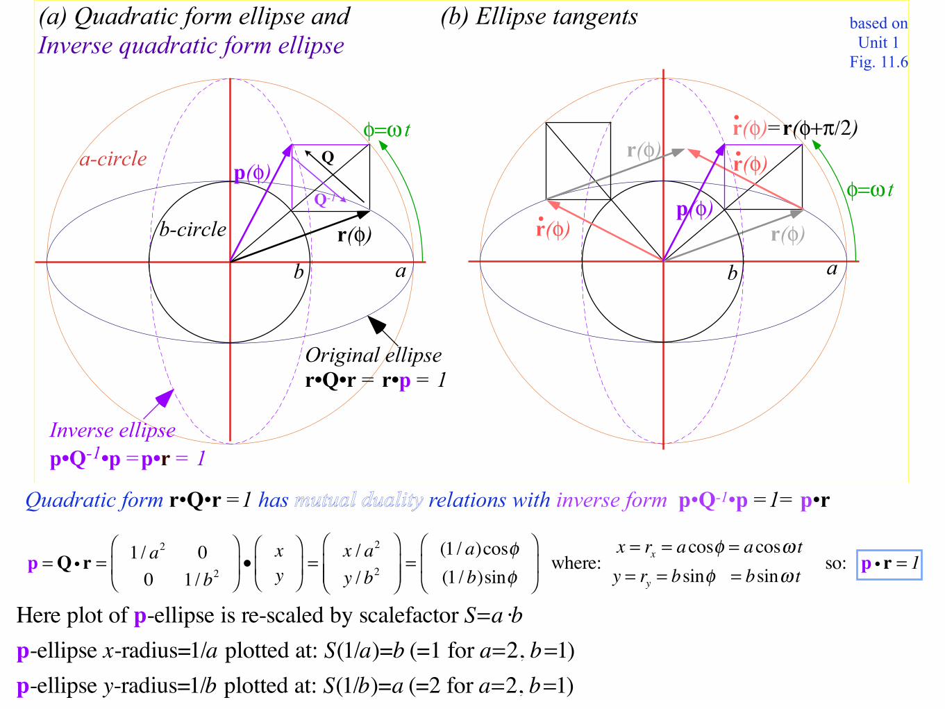
Quadratic form r•Q•r =1 has mutual duality relations with inverse form p•Q-1•p =1= p•r

p = Q• r

r = Q−1•p

Defined mapping between ellipses

Q

Q-1

based on Unit 1

Fig. 11.6

Here plot of p-ellipse is re-scaled by scalefactor S=a ·bp-ellipse x-radius=1/a plotted at: S(1/a)=b (=1 for a=2, b=1)p-ellipse y-radius=1/b plotted at: S(1/b)=a (=2 for a=2, b=1)

r(φ)

φ=ω t

ab

b-circle

a-circle

Original ellipse

r•Q•r = r•p = 1

Inverse ellipse

p•Q-1•p =p•r = 1

p(φ)

(a) Quadratic form ellipse and

Inverse quadratic form ellipse

Quadratic form r•Q•r =1 has mutual duality relations with inverse form p•Q-1•p =1= p•r

p =Q i r = 1/ a2 00 1/ b2

⎛

⎝⎜

⎞

⎠⎟ •

xy

⎛

⎝⎜

⎞

⎠⎟ =

x / a2

y / b2

⎛

⎝⎜⎜

⎞

⎠⎟⎟=

(1 / a)cosφ(1 / b)sinφ

⎛

⎝⎜

⎞

⎠⎟ where:

x = rx = acosφ = acosω ty = ry = bsinφ = bsinω t

so: p i r = 1

p = Q• r

r = Q−1•p

Defined mapping between ellipses

Q

Q-1

based on Unit 1

Fig. 11.6

r pQ

Here plot of p-ellipse is re-scaled by scalefactor S=a ·bp-ellipse x-radius=1/a plotted at: S(1/a)=b (=1 for a=2, b=1)p-ellipse y-radius=1/b plotted at: S(1/b)=a (=2 for a=2, b=1)

Link → IHO orbital time rates of change Link → IHO Exegesis Plot

Link ⇒ BoxIt simulation of IHO orbits

Introduction to dual matrix operator geometry (based on IHO orbits) Quadratic form ellipse r•Q•r=1 vs.inverse form ellipse p•Q -1•p=1

Duality norm relations ( r•p=1) Q-Ellipse tangents r′ normal to dual Q -1-ellipse position p ( r′•p=0=r•p′)

Operator geometric sequences and eigenvectors Alternative scaling of matrix operator geometry

Vector calculus of tensor operation

Quadratic form r•Q•r =1 has mutual duality relations with inverse form p•Q-1•p =1= p•r

p =Q i r = 1/ a2 00 1/ b2

⎛

⎝⎜

⎞

⎠⎟ •

xy

⎛

⎝⎜

⎞

⎠⎟ =

x / a2

y / b2

⎛

⎝⎜⎜

⎞

⎠⎟⎟=

(1 / a)cosφ(1 / b)sinφ

⎛

⎝⎜

⎞

⎠⎟ where:

x = rx = acosφ = acosω ty = ry = bsinφ = bsinω t

so: p i r = 1

r(φ)

φ=ω t

ab

b-circle

a-circle

r(φ)ab

r(φ)=r(φ+π/2)•

r(φ)•r(φ)

Original ellipse

r•Q•r = r•p = 1

p(φ)

Inverse ellipse

p•Q-1•p =p•r = 1

p(φ)

(a) Quadratic form ellipse and

Inverse quadratic form ellipse

(b) Ellipse tangents

r(φ)•

φ=ω tQ

Q-1

based on Unit 1

Fig. 11.6

Here plot of p-ellipse is re-scaled by scalefactor S=a ·bp-ellipse x-radius=1/a plotted at: S(1/a)=b (=1 for a=2, b=1)p-ellipse y-radius=1/b plotted at: S(1/b)=a (=2 for a=2, b=1)

!r •p = 0 = !rx !ry( )• pxpy

⎛

⎝⎜⎜

⎞

⎠⎟⎟= −asinφ bcosφ( )• (1 / a)cosφ

(1 / b)sinφ

⎛

⎝⎜

⎞

⎠⎟ where:

!rx = −asinφ!ry = bcosφ

and:px = (1 / a)cosφ py = (1 / b)sinφ

Quadratic form r•Q•r =1 has mutual duality relations with inverse form p•Q-1•p =1= p•r

p =Q i r = 1/ a2 00 1/ b2

⎛

⎝⎜

⎞

⎠⎟ •

xy

⎛

⎝⎜

⎞

⎠⎟ =

x / a2

y / b2

⎛

⎝⎜⎜

⎞

⎠⎟⎟=

(1 / a)cosφ(1 / b)sinφ

⎛

⎝⎜

⎞

⎠⎟ where:

x = rx = acosφ = acosω ty = ry = bsinφ = bsinω t

so: p i r = 1

r(φ)

φ=ω t

ab

b-circle

a-circle

r(φ)ab

r(φ)=r(φ+π/2)•

r(φ)•r(φ)

Original ellipse

r•Q•r = r•p = 1

p(φ)

vector p(φ) isperpendicular

to r(φ)•Inverse ellipse

p•Q-1•p =p•r = 1

p(φ)

(a) Quadratic form ellipse and

Inverse quadratic form ellipse

(b) Ellipse tangents

r(φ)•

φ=ω t

p is perpendicular to velocity v=r , a mutual orthogonality•

•

Q

Q-1

based on Unit 1

Fig. 11.6

p =Q i r = 1/ a2 00 1/ b2

⎛

⎝⎜

⎞

⎠⎟ •

xy

⎛

⎝⎜

⎞

⎠⎟ =

x / a2

y / b2

⎛

⎝⎜⎜

⎞

⎠⎟⎟=

(1 / a)cosφ(1 / b)sinφ

⎛

⎝⎜

⎞

⎠⎟ where:

x = rx = acosφ = acosω ty = ry = bsinφ = bsinω t

so: p i r = 1

!r •p = 0 = !rx !ry( )• pxpy

⎛

⎝⎜⎜

⎞

⎠⎟⎟= −asinφ bcosφ( )• (1 / a)cosφ

(1 / b)sinφ

⎛

⎝⎜

⎞

⎠⎟ where:

!rx = −asinφ!ry = bcosφ

and:px = (1 / a)cosφ py = (1 / b)sinφ

Quadratic form r•Q•r =1 has mutual duality relations with inverse form p•Q-1•p =1unit

mutual projection

p is perpendicular to velocity v=r , a mutual orthogonality. So is r perpendicular to p: p•r=0•

Unit 1 Fig. 11.6

r(φ)

φ=ω t

ab

b-circle

a-circle

r(φ)ab

r(φ)=r(φ+π/2)•

r(φ)•r(φ)

Original ellipse

r•Q•r = r•p = 1

p(φ)

p(φ)

p(φ)= p(φ+π/2)•

p(φ)•

vector p(φ) isperpendicular

to r(φ)•Inverse ellipse

p•Q-1•p =p•r = 1

p(φ)

(a) Quadratic form ellipse and

Inverse quadratic form ellipse

(b) Ellipse tangents

r(φ)•

φ=ω t

vector p(φ) isperpendicular

to r(φ)

•

• •

•

Q

Q-1

Geometry of dual ellipse Kepler anomalies for vectors [r(φ), p(φ)] and d/dt[r(φ), p(φ),] in coordinate (x,y) space rendered by animation web-app in RelaWavity and described in Lect. 12-advanced.

RelaWavity Web Simulation Ellipse/Exegesis

Introduction to dual matrix operator geometry (based on IHO orbits) Quadratic form ellipse r•Q•r=1 vs.inverse form ellipse p•Q -1•p=1

Duality norm relations ( r•p=1) Q-Ellipse tangents r′ normal to dual Q -1-ellipse position p ( r′•p=0=r•p′)

Operator geometric sequences and eigenvectors Alternative scaling of matrix operator geometry

Vector calculus of tensor operation

Start with 45° unit vector v x/y = xy

⎛

⎝⎜

⎞

⎠⎟ =

1/ 2

1 / 2

⎛

⎝⎜⎜

⎞

⎠⎟⎟

.

based on Fig. 11.7 in Unit 1Here b/a=1/2

Diagonal R-matrix acts on vector v x/y . Resulting vector has slope changed by factor a /b = 2.

R i v x/y =1/a 00 1/b

⎛

⎝⎜⎜

⎞

⎠⎟⎟

xy

⎛

⎝⎜

⎞

⎠⎟ =

x/ay/b

⎛

⎝⎜⎜

⎞

⎠⎟⎟

(Slope increases if a >b.)

Diagonal R−1-matrix acts on vector v x/y . Resulting vector has slope changed by factor b/a.

R−1 i v x/y = a 00 b

⎛⎝⎜

⎞⎠⎟

xy

⎛

⎝⎜

⎞

⎠⎟ =

x ⋅ay ⋅b

⎛

⎝⎜

⎞

⎠⎟

(Slope decreases if b< a.)

based on Fig. 11.7 in Unit 1Here b/a=1/2

Action of “sqrt-1-”matrix R -1 =√Q -1

Action of “sqrt-”matrix R=√Q

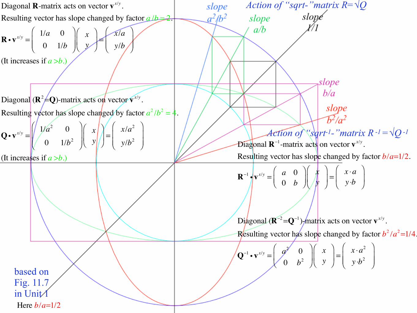
Diagonal (R2=Q)-matrix acts on vector v x/y . Resulting vector has slope changed by factor a2 /b2 = 4.

Q i v x/y =1/a2 0

0 1/b2

⎛

⎝⎜⎜

⎞

⎠⎟⎟

xy

⎛

⎝⎜

⎞

⎠⎟ =

x/a2

y/b2

⎛

⎝⎜⎜

⎞

⎠⎟⎟

(It increases if a >b.)

Diagonal (R−2=Q−1)-matrix acts on vector v x/y . Resulting vector has slope changed by factor b2 /a2=1/4.

Q−1 i v x/y = a2 00 b2

⎛

⎝⎜

⎞

⎠⎟

xy

⎛

⎝⎜

⎞

⎠⎟ =

x ⋅a2

y ⋅b2

⎛

⎝⎜⎜

⎞

⎠⎟⎟

Diagonal R-matrix acts on vector v x/y . Resulting vector has slope changed by factor a /b = 2.

R i v x/y =1/a 00 1/b

⎛

⎝⎜⎜

⎞

⎠⎟⎟

xy

⎛

⎝⎜

⎞

⎠⎟ =

x/ay/b

⎛

⎝⎜⎜

⎞

⎠⎟⎟

(It increases if a >b.)

Diagonal R−1-matrix acts on vector v x/y . Resulting vector has slope changed by factor b/a=1/2.

R−1 i v x/y = a 00 b

⎛⎝⎜

⎞⎠⎟

xy

⎛

⎝⎜

⎞

⎠⎟ =

x ⋅ay ⋅b

⎛

⎝⎜

⎞

⎠⎟

based on Fig. 11.7 in Unit 1Here b/a=1/2

Action of “sqrt-1-”matrix R -1 =√Q -1

Action of “sqrt-”matrix R=√Q

slope1/1

slopea/b

slopeb/aslopeb2/a2

slopea2/b2

slopeb3/a3

slopea3/b3

Diagonal (R2=Q)-matrix acts on vector v x/y . Resulting vector has slope changed by factor a2 /b2 = 4.

Q i v x/y =1/a2 0

0 1/b2

⎛

⎝⎜⎜

⎞

⎠⎟⎟

xy

⎛

⎝⎜

⎞

⎠⎟ =

x/a2

y/b2

⎛

⎝⎜⎜

⎞

⎠⎟⎟

(It increases if a >b.)

Diagonal R-matrix acts on vector v x/y . Resulting vector has slope changed by factor a /b = 2.

R i v x/y =1/a 00 1/b

⎛

⎝⎜⎜

⎞

⎠⎟⎟

xy

⎛

⎝⎜

⎞

⎠⎟ =

x/ay/b

⎛

⎝⎜⎜

⎞

⎠⎟⎟

(It increases if a >b.)

Either process can go on forever... Diagonal (R2n=Qn )-matrix acts on vector v x/y . Resulting vector has slope changed by factor a2n /b2n = 4n.

Either process can go on forever... Diagonal (R−2n=Q−n )-matrix acts on vector v x/y . Resulting vector has slope changed by factor b2n /a2n = 4−n.

based on Fig. 11.7 in Unit 1Here b/a=1/2

slope1/1

slopea/b

slopeb/aslopeb2/a2

slopea2/b2

slopeb3/a3

slopea3/b3

Diagonal (R2=Q)-matrix acts on vector v x/y . Resulting vector has slope changed by factor a2 /b2 = 4.

Q i v x/y =1/a2 0

0 1/b2

⎛

⎝⎜⎜

⎞

⎠⎟⎟

xy

⎛

⎝⎜

⎞

⎠⎟ =

x/a2

y/b2

⎛

⎝⎜⎜

⎞

⎠⎟⎟

(It increases if a >b.)

Diagonal R-matrix acts on vector v x/y . Resulting vector has slope changed by factor a /b = 2.

R i v x/y =1/a 00 1/b

⎛

⎝⎜⎜

⎞

⎠⎟⎟

xy

⎛

⎝⎜

⎞

⎠⎟ =

x/ay/b

⎛

⎝⎜⎜

⎞

⎠⎟⎟

(It increases if a >b.)

Either process can go on forever... Diagonal (R2n=Qn )-matrix acts on vector v x/y . Resulting vector has slope changed by factor a2n /b2n = 4n.

...Finally, the result approaches EIGENVECTOR y = 01

⎛⎝⎜

⎞⎠⎟

of ∞-slope which is "immune" to R , Q or Qn : R y = (1/b) y Qn y = (1/b2 )n y

Either process can go on forever... Diagonal (R−2n=Q−n )-matrix acts on vector v x/y . Resulting vector has slope changed by factor b2n /a2n = 4−n.

...Finally, the result approaches EIGENVECTOR x = 10

⎛⎝⎜

⎞⎠⎟

of 0-slope which is "immune" to R−1 , Q−1 or Q−n : R−1 x = (a) x Q−n x = (a2 )n x

EIGENVECTOR y

EIGENVECTOR x

Here b/a=1/2

slope1/1

slopea/b

slopeb/aslopeb2/a2

slopea2/b2

slopeb3/a3

slopea3/b3

Diagonal (R2=Q)-matrix acts on vector v x/y . Resulting vector has slope changed by factor a2 /b2 = 4.

Q i v x/y =1/a2 0

0 1/b2

⎛

⎝⎜⎜

⎞

⎠⎟⎟

xy

⎛

⎝⎜

⎞

⎠⎟ =

x/a2

y/b2

⎛

⎝⎜⎜

⎞

⎠⎟⎟

(It increases if a >b.)

Diagonal R-matrix acts on vector v x/y . Resulting vector has slope changed by factor a /b = 2.

R i v x/y =1/a 00 1/b

⎛

⎝⎜⎜

⎞

⎠⎟⎟

xy

⎛

⎝⎜

⎞

⎠⎟ =

x/ay/b

⎛

⎝⎜⎜

⎞

⎠⎟⎟

(It increases if a >b.)

Either process can go on forever... Diagonal (R2n=Qn )-matrix acts on vector v x/y . Resulting vector has slope changed by factor a2n /b2n = 4n.

...Finally, the result approaches EIGENVECTOR y = 01

⎛⎝⎜

⎞⎠⎟

of ∞-slope which is "immune" to R , Q or Qn : R y = (1/b) y Qn y = (1/b2 )n y

Either process can go on forever... Diagonal (R−2n=Q−n )-matrix acts on vector v x/y . Resulting vector has slope changed by factor b2n /a2n = 4−n.

...Finally, the result approaches EIGENVECTOR x = 10

⎛⎝⎜

⎞⎠⎟

of 0-slope which is "immune" to R−1 , Q−1 or Q−n : R−1 x = (a) x Q−n x = (a2 )n x

EIGENVECTOR y

EIGENVECTOR x

Eigensolution RelationsEigenvalues Eigenvalues

Here b/a=1/2

Introduction to dual matrix operator geometry (based on IHO orbits) Quadratic form ellipse r•Q•r=1 vs.inverse form ellipse p•Q -1•p=1

Duality norm relations ( r•p=1) Q-Ellipse tangents r′ normal to dual Q -1-ellipse position p ( r′•p=0=r•p′)

Operator geometric sequences and eigenvectors Alternative scaling of matrix operator geometry

Vector calculus of tensor operation

Start with 45° unit vector v x/y = xy

⎛

⎝⎜

⎞

⎠⎟ =

1/ 2

1 / 2

⎛

⎝⎜⎜

⎞

⎠⎟⎟

.

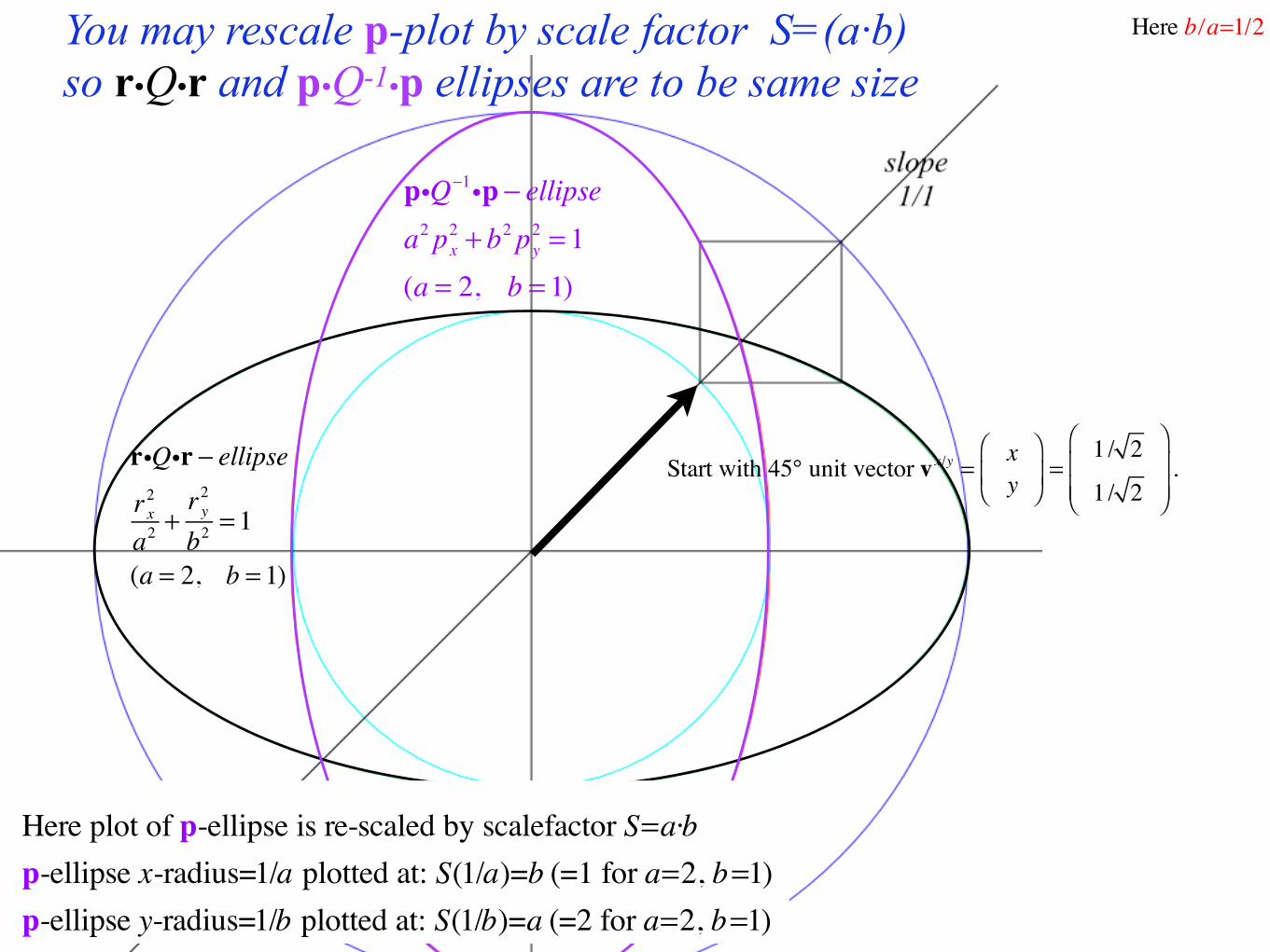
You may rescale p-plot by scale factor S=(a·b) so r•Q•r and p•Q-1•p ellipses are to be same size

riQir − ellipse

r2xa2

+r2yb2

= 1

(a = 2, b = 1)

piQ−1ip − ellipsea2p2x + b

2p2y = 1(a = 2, b = 1)

Here b/a=1/2

Here plot of p-ellipse is re-scaled by scalefactor S=a·bp-ellipse x-radius=1/a plotted at: S(1/a)=b (=1 for a=2, b=1)p-ellipse y-radius=1/b plotted at: S(1/b)=a (=2 for a=2, b=1)

Start with 45° unit vector v x/y = xy

⎛

⎝⎜

⎞

⎠⎟ =

1/ 2

1 / 2

⎛

⎝⎜⎜

⎞

⎠⎟⎟

.

riQir − ellipse

r2xa2

+r2yb2

= 1

(a = 2, b = 1)

piQ−1ip − ellipsea2p2x + b

2p2y = 1(a = 2, b = 1)

1/a = 1/ 2

2

b = 1

a = 2

1/b = 1

Here b/a=1/2..or else rescale p-plot by scale factor S=b to separate r•Q•r and p•Q-1•p ellipses into different regions

Here plot of p-ellipse is re-scaled by scalefactor S=bp-ellipse x-radius=1/a plotted at: S(1/a)=b/a (=1/2 for a=2, b=1)p-ellipse y-radius=1/b plotted at: S(1/b)=1

|r|≥1 and |p|≤1

slopeb/a=1/2

r•Q•r-ellipserx2/a2+ry

2/b2=1(a = 2.0 , b = =1.0 )

p•Q-1•p-ellipsea2px

2+b2py2=1

(a = 2.0 , b = =1.0 )

b=1.0

p(φ1) = Q i r(φ−1)

= 1/ a2 0

0 1/ b2

⎛

⎝⎜⎜

⎞

⎠⎟⎟

acosφ0

bsinφ0

⎛

⎝⎜⎜

⎞

⎠⎟⎟

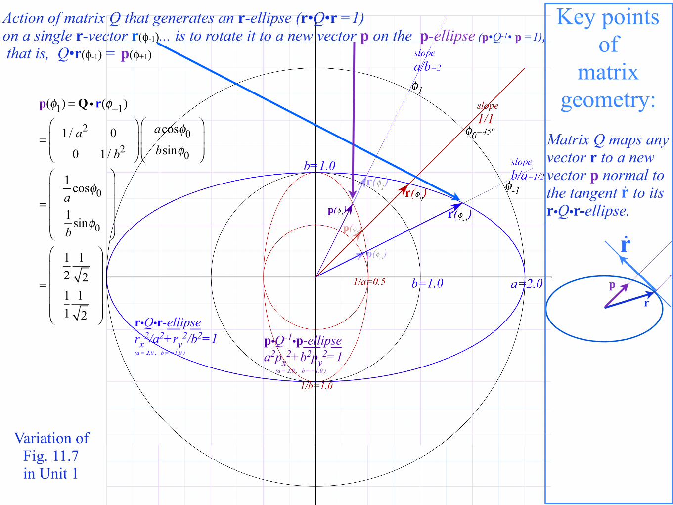
Action of matrix Q that generates an r-ellipse (r•Q• r =1) on a single r-vector r(φ-1)...

acosφ0

bsinφ0

r(φ-1)φ0

φ-1

a

b

Variation of Fig. 11.7 in Unit 1

Here plot of p-ellipse is re-scaled by scalefactor S=bp-ellipse x-radius=1/a plotted at: S(1/a)=b/a (=1/2 for a=2, b=1)p-ellipse y-radius=1/b plotted at: S(1/b)=1

slopeb/a=1/2

r•Q•r-ellipserx2/a2+ry

2/b2=1(a = 2.0 , b = =1.0 )

p•Q-1•p-ellipsea2px

2+b2py2=1

(a = 2.0 , b = =1.0 )

b=1.0

p(φ1) = Q i r(φ−1)

= 1/ a2 0

0 1/ b2

⎛

⎝⎜⎜

⎞

⎠⎟⎟

acosφ0

bsinφ0

⎛

⎝⎜⎜

⎞

⎠⎟⎟

=

1a

cosφ0

1b

sinφ0

⎛

⎝

⎜⎜⎜⎜

⎞

⎠

⎟⎟⎟⎟

=

12

1

211

1

2

⎛

⎝

⎜⎜⎜⎜⎜

⎞

⎠

⎟⎟⎟⎟⎟

Action of matrix Q that generates an r-ellipse (r•Q•r =1) on a single r-vector r(φ-1)... is to rotate it to a new vector p on the p-ellipse (p•Q-1• p =1), that is, Q•r(φ-1) = p(φ+1)

Variation of Fig. 11.7 in Unit 1

slopeb/a=1/2

r•Q•r-ellipserx2/a2+ry

2/b2=1(a = 2.0 , b = =1.0 )

p•Q-1•p-ellipsea2px

2+b2py2=1

(a = 2.0 , b = =1.0 )

b=1.0

p(φ1) = Q i r(φ−1)

= 1/ a2 0

0 1/ b2

⎛

⎝⎜⎜

⎞

⎠⎟⎟

acosφ0

bsinφ0

⎛

⎝⎜⎜

⎞

⎠⎟⎟

=

1a

cosφ0

1b

sinφ0

⎛

⎝

⎜⎜⎜⎜

⎞

⎠

⎟⎟⎟⎟

=

12

1

211

1

2

⎛

⎝

⎜⎜⎜⎜⎜

⎞

⎠

⎟⎟⎟⎟⎟

Action of matrix Q that generates an r-ellipse (r•Q•r =1) on a single r-vector r(φ-1)... is to rotate it to a new vector p on the p-ellipse (p•Q-1• p =1), that is, Q•r(φ-1) = p(φ+1)

Key points of

matrix geometry:

Matrix Q maps any vector r to a new vector p normal to the tangent to its r•Q•r-ellipse.

rp

!r

!r

Variation of Fig. 11.7 in Unit 1

slopeb/a=1/2

r•Q•r-ellipserx2/a2+ry

2/b2=1(a = 2.0 , b = =1.0 )

p•Q-1•p-ellipsea2px

2+b2py2=1

(a = 2.0 , b = =1.0 )

b=1.0

p(φ1) = Q i r(φ−1)

= 1/ a2 0

0 1/ b2

⎛

⎝⎜⎜

⎞

⎠⎟⎟

acosφ0

bsinφ0

⎛

⎝⎜⎜

⎞

⎠⎟⎟

=

1a

cosφ0

1b

sinφ0

⎛

⎝

⎜⎜⎜⎜

⎞

⎠

⎟⎟⎟⎟

=

12

1

211

1

2

⎛

⎝

⎜⎜⎜⎜⎜

⎞

⎠

⎟⎟⎟⎟⎟

Action of matrix Q that generates an r-ellipse (r•Q•r =1) on a single r-vector r(φ-1)... is to rotate it to a new vector p on the p-ellipse (p•Q-1• p =1), that is, Q•r(φ-1) = p(φ+1)

Key points of

matrix geometry:

Matrix Q maps any vector r to a new vector p normal to the tangent to its r•Q•r-ellipse.

rp

!r

!r

Matrix Q-1 maps p back to r that is normal to the tangent to its p• Q-1• p-ellipse.

!p

!p

!p

Variation of Fig. 11.7 in Unit 1

Introduction to dual matrix operator geometry (based on IHO orbits) Quadratic form ellipse r•Q•r=1 vs.inverse form ellipse p•Q -1•p=1

Duality norm relations ( r•p=1) Q-Ellipse tangents r′ normal to dual Q -1-ellipse position p ( r′•p=0=r•p′)

Operator geometric sequences and eigenvectors Alternative scaling of matrix operator geometry

Vector calculus of tensor operation

Derive matrix “normal-to-ellipse”geometry by vector calculus: Let matrix Q =

define the ellipse 1=r•Q•r =

A BB D

⎛⎝⎜

⎞⎠⎟

x y( ) i A BB D

⎛⎝⎜

⎞⎠⎟

ixy

⎛

⎝⎜

⎞

⎠⎟ = x y( ) i A ⋅ x + B ⋅ y

B ⋅ x + D ⋅ y

⎛

⎝⎜

⎞

⎠⎟ = A ⋅ x2 + 2B ⋅ xy + D ⋅ y2 = 1

rp

!rrp

!r

B = 0 B ≠ 0

Derive matrix “normal-to-ellipse”geometry by vector calculus: Let matrix Q =

define the ellipse 1=r•Q•r =

Compare operation by Q on vector r with vector derivative or gradient of r•Q•r

A BB D

⎛⎝⎜

⎞⎠⎟

x y( ) i A BB D

⎛⎝⎜

⎞⎠⎟

ixy

⎛

⎝⎜

⎞

⎠⎟ = x y( ) i A ⋅ x + B ⋅ y

B ⋅ x + D ⋅ y

⎛

⎝⎜

⎞

⎠⎟ = A ⋅ x2 + 2B ⋅ xy + D ⋅ y2 = 1

rp

!rrp

!r

A BB D

⎛⎝⎜

⎞⎠⎟

ixy

⎛

⎝⎜

⎞

⎠⎟ =

A ⋅ x + B ⋅ yB ⋅ x + D ⋅ y

⎛

⎝⎜

⎞

⎠⎟

∂∂rr iQ i r( ) = ∇ r iQ i r( )

∂∂x∂∂y

⎛

⎝

⎜⎜⎜⎜

⎞

⎠

⎟⎟⎟⎟

A ⋅ x2 + 2B ⋅ xy + D ⋅ y2( ) = 2A ⋅ x + 2B ⋅ y2B ⋅ x + 2D ⋅ y

⎛

⎝⎜

⎞

⎠⎟

B = 0 B ≠ 0

Derive matrix “normal-to-ellipse”geometry by vector calculus: Let matrix Q =

define the ellipse 1=r•Q•r =

Compare operation by Q on vector r with vector derivative or gradient of r•Q•r

A BB D

⎛⎝⎜

⎞⎠⎟

x y( ) i A BB D

⎛⎝⎜

⎞⎠⎟

ixy

⎛

⎝⎜

⎞

⎠⎟ = x y( ) i A ⋅ x + B ⋅ y

B ⋅ x + D ⋅ y

⎛

⎝⎜

⎞

⎠⎟ = A ⋅ x2 + 2B ⋅ xy + D ⋅ y2 = 1

rp

!rrp

!r

Very simple result:

A BB D

⎛⎝⎜

⎞⎠⎟

ixy

⎛

⎝⎜

⎞

⎠⎟ =

A ⋅ x + B ⋅ yB ⋅ x + D ⋅ y

⎛

⎝⎜

⎞

⎠⎟

∂∂rr iQ i r( ) = ∇ r iQ i r( )

∂∂x∂∂y

⎛

⎝

⎜⎜⎜⎜

⎞

⎠

⎟⎟⎟⎟

A ⋅ x2 + 2B ⋅ xy + D ⋅ y2( ) = 2A ⋅ x + 2B ⋅ y2B ⋅ x + 2D ⋅ y

⎛

⎝⎜

⎞

⎠⎟

∂∂r

r iQ i r2

⎛⎝⎜

⎞⎠⎟ = ∇ r iQ i r

2⎛⎝⎜

⎞⎠⎟ =Q i r

B = 0 B ≠ 0

Introduction to dual matrix operator geometry (based on IHO orbits) Quadratic form ellipse r•Q•r=1 vs.inverse form ellipse p•Q -1•p=1

Duality norm relations ( r•p=1) Q-Ellipse tangents r′ normal to dual Q -1-ellipse position p ( r′•p=0=r•p′)

(Still more) Operator geometric sequences and eigenvectors Alternative scaling of matrix operator geometry

Vector calculus of tensor operation

slopeb/a=1/2

r•Q•r-ellipserx2/a2+ry

2/b2=1(a = 2.0 , b = =1.0 )

p•Q-1•p-ellipsea2px

2+b2py2=1

(a = 2.0 , b = =1.0 )

b=1.0

u = Q i r(φ−1) = R i r(φ−1)

= 1/ a 00 1/ b

⎛

⎝⎜⎞

⎠⎟acosφ0

bsinφ0

⎛

⎝⎜⎜

⎞

⎠⎟⎟

=

1a

acosφ0

1b

bsinφ0

⎛

⎝

⎜⎜⎜⎜

⎞

⎠

⎟⎟⎟⎟

=cosφ0

sinφ0

⎛

⎝⎜⎜

⎞

⎠⎟⎟

=

1

21

2

⎛

⎝

⎜⎜⎜⎜⎜

⎞

⎠

⎟⎟⎟⎟⎟

Action of “sqrt-”matrix R=√Q (R generates another ellipse r•R•r =1 not shown) on a single r-vector r(φ-1)... is to rotate it to u-circle (u•u =1), that is, R•r(φ-1) = u =(const.)r(φ0)

a unit vector on unit-circle

u

Variation of Fig. 11.7 in Unit 1

slopeb2/a2

As before, these processes may be continued indefinitely.

Variation of Fig. 11.7 in Unit 1

slopeb2/a2

...And includes a cool way to construct those tangents ... etc. (see exercises!)

!r(φ−2 )

!r(φ−2 )

!p(φ1)

!p(φ1)

Variation of Fig. 11.7 in Unit 1

Q:Where is this headed? A: Lagrangian-Hamiltonian duality Preview of Lecture 8

(a) Lagrangian L = L(v1,v2)

v1

v2(b) Estrangian E = E(V1,V2)

V1=√m1v1

(c) Hamiltonian H = H(p1,p2)

p1=m1v1

p2=m2v2

V2=√m2v2

COM Bisectorslope = 1/1

Collision line andCOM tangent slope= -m1/m2 =-16

Collision line andCOM tangent slope=-√m1/√m2=-4

COM Bisector slope= √m2/√m1 =1/4

Collision line andCOM tangent slope

= -1/1

COM Bisector slope= m2/m1 =1/16

slope√m1√m2

=4

slope=1

The R and Q matrix transformations are like the mechanics rescaling matrices √M and M: Like Q=R2: Like √Q=R: Like Q-1=R-2:

M =m1 00 m2

⎛

⎝⎜⎜

⎞

⎠⎟⎟= R2

M =m1 0

0 m2

⎛

⎝⎜⎜

⎞

⎠⎟⎟= R M−1 =

1/m1 00 1 /m2

⎛

⎝⎜⎜

⎞

⎠⎟⎟= R−2

Unit 1 Fig. 12.1

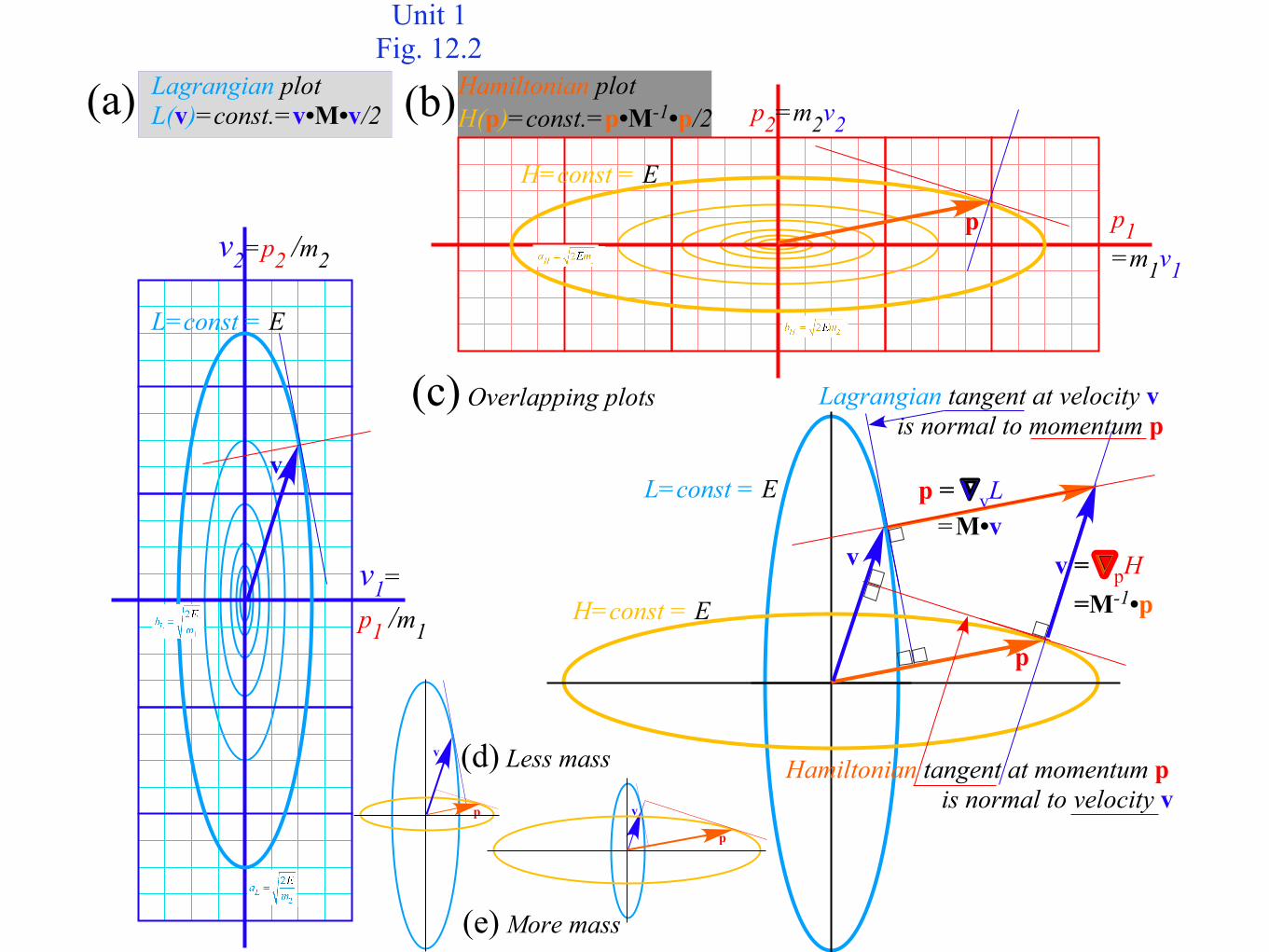
p2=m2v2

p1=m1v1

Hamiltonian plotH(p)=const.=p•M-1•p/2(b)Lagrangian plot

L(v)=const.=v•M•v/2

v2=p2 /m2

L=const = E

v1=p1 /m1

(a)

v v = ∇∇pH=M-1•p

p = ∇∇vL=M•v

p

Lagrangian tangent at velocity vis normal to momentum p

Hamiltonian tangent at momentum pis normal to velocity v

(c) Overlapping plotsv

p

v

p

p

v (d) Less mass

(e) More mass

H=const = E

L=const = E

H=const = E

Unit 1 Fig. 12.2

AMOP reference links (Updated list given on 2nd and 3rd pages of each class presentation)

Representaions Of Multidimensional Symmetries In Networks - harter-jmp-1973Alternative Basis for the Theory of Complex Spectra

Alternative_Basis_for_the_Theory_of_Complex_Spectra_I_-_harter-pra-1973Alternative_Basis_for_the_Theory_of_Complex_Spectra_II_-_harter-patterson-pra-1976Alternative_Basis_for_the_Theory_of_Complex_Spectra_III_-_patterson-harter-pra-1977

Frame Transformation Relations And Multipole Transitions In Symmetric Polyatomic Molecules - RMP-1978Asymptotic eigensolutions of fourth and sixth rank octahedral tensor operators - Harter-Patterson-JMP-1979Rotational energy surfaces and high- J eigenvalue structure of polyatomic molecules - Harter - Patterson - 1984Galloping waves and their relativistic properties - ajp-1985-HarterRovibrational Spectral Fine Structure Of Icosahedral Molecules - Cpl 1986 (Alt Scan)Theory of hyperfine and superfine levels in symmetric polyatomic molecules.

I) Trigonal and tetrahedral molecules: Elementary spin-1/2 cases in vibronic ground states - PRA-1979-Harter-Patterson (Alt scan)II) Elementary cases in octahedral hexafluoride molecules - Harter-PRA-1981 (Alt scan)

Rotation–vibration spectra of icosahedral molecules. I) Icosahedral symmetry analysis and fine structure - harter-weeks-jcp-1989 (Alt scan)II) Icosahedral symmetry, vibrational eigenfrequencies, and normal modes of buckminsterfullerene - weeks-harter-jcp-1989 (Alt scan)III) Half-integral angular momentum - harter-reimer-jcp-1991

Rotation-vibration scalar coupling zeta coefficients and spectroscopic band shapes of buckminsterfullerene - Weeks-Harter-CPL-1991 (Alt scan)Nuclear spin weights and gas phase spectral structure of 12C60 and 13C60 buckminsterfullerene -Harter-Reimer-Cpl-1992 - (Alt1, Alt2 Erratum)Gas Phase Level Structure of C60 Buckyball and Derivatives Exhibiting Broken Icosahedral Symmetry - reimer-diss-1996Fullerene symmetry reduction and rotational level fine structure/ the Buckyball isotopomer 12C 13C59 - jcp-Reimer-Harter-1997 (HiRez)Wave Node Dynamics and Revival Symmetry in Quantum Rotors - harter - jms - 2001Molecular Symmetry and Dynamics - Ch32-Springer Handbooks of Atomic, Molecular, and Optical Physics - Harter-2006Resonance and Revivals

I) QUANTUM ROTOR AND INFINITE-WELL DYNAMICS - ISMSLi2012 (Talk) OSU knowledge BankII) Comparing Half-integer Spin and Integer Spin - Alva-ISMS-Ohio2013-R777 (Talks)III) Quantum Resonant Beats and Revivals in the Morse Oscillators and Rotors - (2013-Li-Diss)

Resonance and Revivals in Quantum Rotors - Comparing Half-integer Spin and Integer Spin - Alva-ISMS-Ohio2013-R777 (Talk)Molecular Eigensolution Symmetry Analysis and Fine Structure - IJMS-harter-mitchell-2013Quantum Revivals of Morse Oscillators and Farey-Ford Geometry - Li-Harter-cpl-2013QTCA Unit 10 Ch 30 - 2013AMOP Ch 0 Space-Time Symmetry - 2019

Web Resources - front page 2014 AMOP

2018 AMOPUAF Physics UTube channel 2017 Group Theory for QM

Classical Mechanics with a Bang!Principles of Symmetry, Dynamics, and Spectroscopy

Quantum Theory for the Computer Age

Modern Physics and its Classical Foundations

*Index/Search is disabled - a web based A.M.O.P. oriented reference page, with thumbnail/previews, greater control over the information display, https://modphys.hosted.uark.edu/markup/AMOP_References.html

and eventually full on Apache-SOLR Index and search for nuanced, whole-site content/metadata level searching.

AMOP reference links (Updated list given on 2nd and 3rd pages of each class presentation)

H atom hyperfine-B-level crossing Unit 8 Ch. 24 p15

Intro spin ½ coupling Unit 8 Ch. 24 p3

Hyperf. theory Ch. 24 p48.

Intro 2p3p coupling Unit 8 Ch. 24 p17. Intro LS-jj coupling Unit 8 Ch. 24 p22.

CG coupling derived (start) Unit 8 Ch. 24 p39.

CG coupling derived (formula) Unit 8 Ch. 24 p44.

Hyperf. theory Ch. 24 p48. Deeper theory ends p53

Lande’ g-factor Unit 8 Ch. 24 p26.

Irrep Tensor building Unit 8 Ch. 25 p5.

Irrep Tensor Tables Unit 8 Ch. 25 p12.

Tensors Applied to d,f-levels. Unit 8 Ch. 25 p21.

Wigner-Eckart tensor Theorem. Unit 8 Ch. 25 p17.

Tensors Applied to high J levels. Unit 8 Ch. 25 p63.

Intro 3-particle coupling. Unit 8 Ch. 25 p28.

Intro 3,4-particle Young Tableaus GrpThLect29 p42.

Young Tableau Magic Formulae GrpThLect29 p46-48.

Int.J.Mol.Sci, 14, 714(2013), QTCA Unit 8 Ch. 23-25, QTCA Unit 9 Ch. 26, PSDS Ch. 5, PSDS Ch. 7

(Int.J.Mol.Sci, 14, 714(2013) p.755-774 , QTCA Unit 7 Ch. 23-26 ), (PSDS - Ch. 5, 7 )

*Index/Search is disabled - a web based A.M.O.P. oriented reference page, with thumbnail/previews, greater control over the information display, https://modphys.hosted.uark.edu/markup/AMOP_References.html

and eventually full on Apache-SOLR Index and search for nuanced, whole-site content/metadata level searching.

Predrag Cvitanovic’s: Birdtrack Notation, Calculations, and SimplificationChaos_Classical_and_Quantum_-_2018-Cvitanovic-ChaosBook

Group Theory - PUP_Lucy_Day_-_Diagrammatic_notation_-_Ch4Simplification_Rules_for_Birdtrack_Operators_-_Alcock-Zeilinger-Weigert-zeilinger-jmp-2017

Group Theory - Birdtracks_Lies_and_Exceptional_Groups_-_Cvitanovic-2011Simplification_rules_for_birdtrack_operators-_jmp-alcock-zeilinger-2017

Birdtracks for SU(N) - 2017-Keppeler

Frank Rioux’s: UMA method of vibrational inductionQuantum_Mechanics_Group_Theory_and_C60_-_Frank_Rioux_-_Department_of_Chemistry_Saint_Johns_U

Symmetry_Analysis_for_H20-_H20GrpTheory-_RiouxQuantum_Mechanics-Group_Theory_and_C60_-_JChemEd-Rioux-1994

Group_Theory_Problems-_Rioux-_SymmetryProblemsXComment_on_the_Vibrational_Analysis_for_C60_and_Other_Fullerenes_Rioux-RSP

Supplemental AMOP Techniques & ExperimentMany Correlation Tables are Molien Sequences - Klee (Draft 2016)

High-resolution_spectroscopy_and_global_analysis_of_CF4_rovibrational_bands_to_model_its_atmospheric_absorption-_carlos-Boudon-jqsrt-2017Symmetry and Chirality - Continuous_Measures_-_Avnir

*Special Topics & Colloquial References

r-process_nucleosynthesis_from_matter_ejected_in_binary_neutron_star_mergers-PhysRevD-Bovard-2017

AMOP reference links (Updated list given on 2nd and 3rd and 4th pages of each class presentation)

*Index/Search is disabled - a web based A.M.O.P. oriented reference page, with thumbnail/previews, greater control over the information display, https://modphys.hosted.uark.edu/markup/AMOP_References.html

and eventually full on Apache-SOLR Index and search for nuanced, whole-site content/metadata level searching.