2015年7月1日星期三 2015年7月1日星期三 2015年7月1日星期三 Data Mining: Concepts and...
114
2022年3年11年 Data Mining: Concepts and Tec hniques 1 Mining Frequent Patterns ©Jiawei Han and Micheline Kamber http://www-sal.cs.uiuc.edu/~hanj/bk2/ Chp 5, Chp 8.3 modified by Donghui Zhang
-
Upload
francis-mcdaniel -
Category
Documents
-
view
412 -
download
1
Transcript of 2015年7月1日星期三 2015年7月1日星期三 2015年7月1日星期三 Data Mining: Concepts and...

2023年4月19日Data Mining: Concepts and Technique
s 1
Mining Frequent Patterns
©Jiawei Han and Micheline Kamber
http://www-sal.cs.uiuc.edu/~hanj/bk2/
Chp 5, Chp 8.3
modified by Donghui Zhang
2023年4月19日Data Mining: Concepts and Technique
s 2
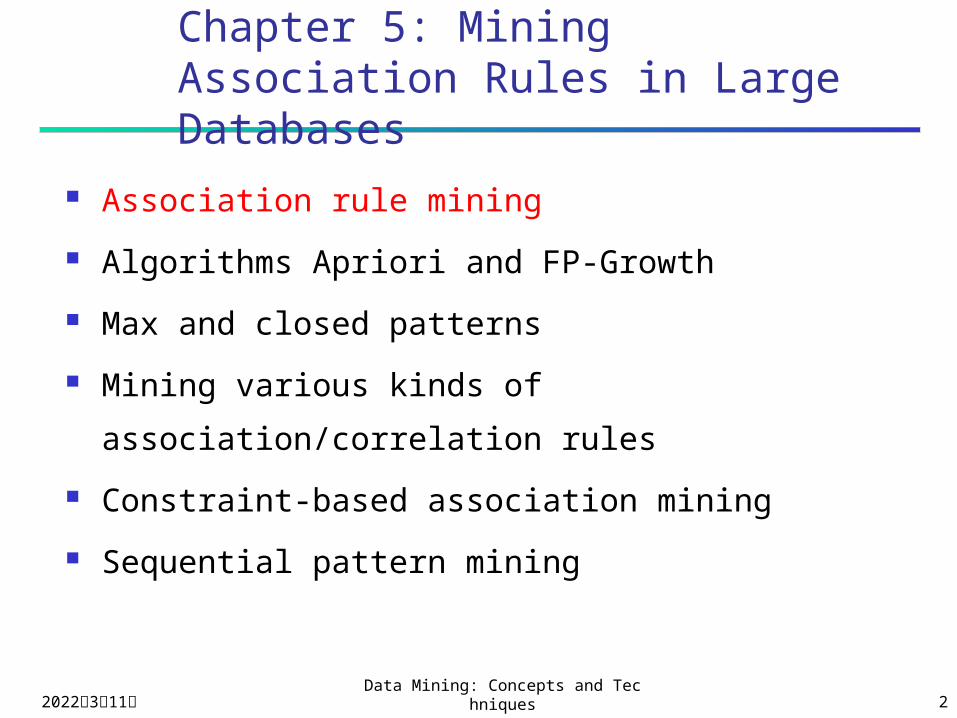
Chapter 5: Mining Association Rules in Large Databases
Association rule mining
Algorithms Apriori and FP-Growth
Max and closed patterns
Mining various kinds of association/correlation
rules
Constraint-based association mining
Sequential pattern mining
2023年4月19日Data Mining: Concepts and Technique
s 3
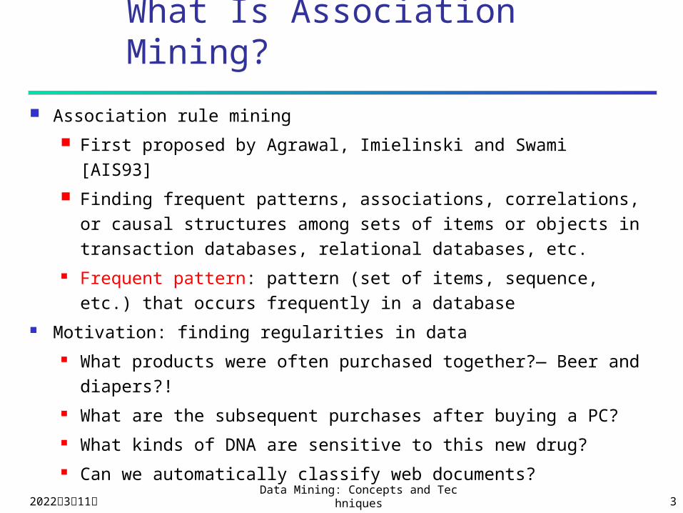
What Is Association Mining?
Association rule mining
First proposed by Agrawal, Imielinski and Swami [AIS93]
Finding frequent patterns, associations, correlations, or causal structures among sets of items or objects in transaction databases, relational databases, etc.
Frequent pattern: pattern (set of items, sequence, etc.) that occurs frequently in a database
Motivation: finding regularities in data What products were often purchased together?— Beer
and diapers?! What are the subsequent purchases after buying a PC? What kinds of DNA are sensitive to this new drug? Can we automatically classify web documents?
2023年4月19日Data Mining: Concepts and Technique
s 4
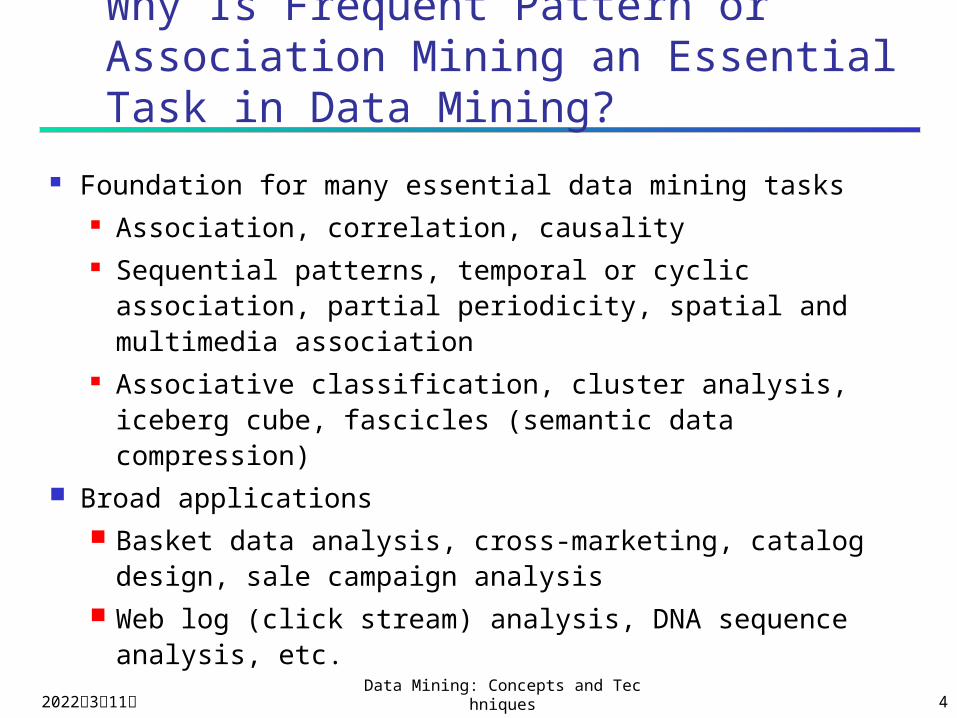
Why Is Frequent Pattern or Association Mining an Essential Task in Data Mining?
Foundation for many essential data mining tasks Association, correlation, causality Sequential patterns, temporal or cyclic association,
partial periodicity, spatial and multimedia association
Associative classification, cluster analysis, iceberg cube, fascicles (semantic data compression)
Broad applications Basket data analysis, cross-marketing, catalog
design, sale campaign analysis Web log (click stream) analysis, DNA sequence
analysis, etc.
2023年4月19日Data Mining: Concepts and Technique
s 5
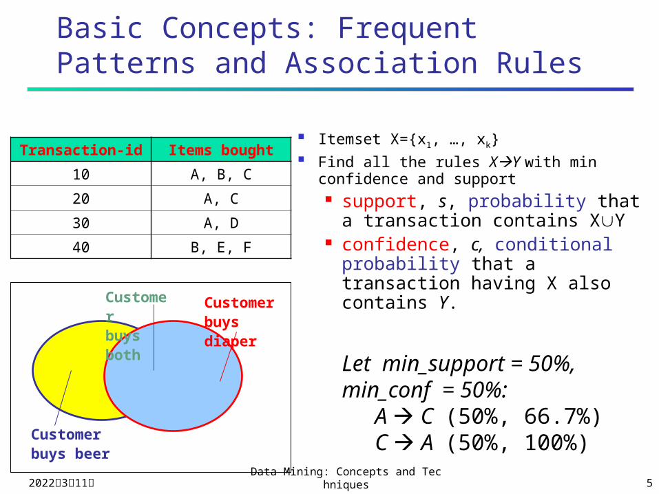
Basic Concepts: Frequent Patterns and Association Rules
Itemset X={x1, …, xk} Find all the rules XY with min
confidence and support support, s, probability that a
transaction contains XY confidence, c, conditional
probability that a transaction having X also contains Y.
Let min_support = 50%, min_conf = 50%:
A C (50%, 66.7%)C A (50%, 100%)
Customerbuys diaper
Customerbuys both
Customerbuys beer
Transaction-id Items bought
10 A, B, C
20 A, C
30 A, D
40 B, E, F
2023年4月19日Data Mining: Concepts and Technique
s 6
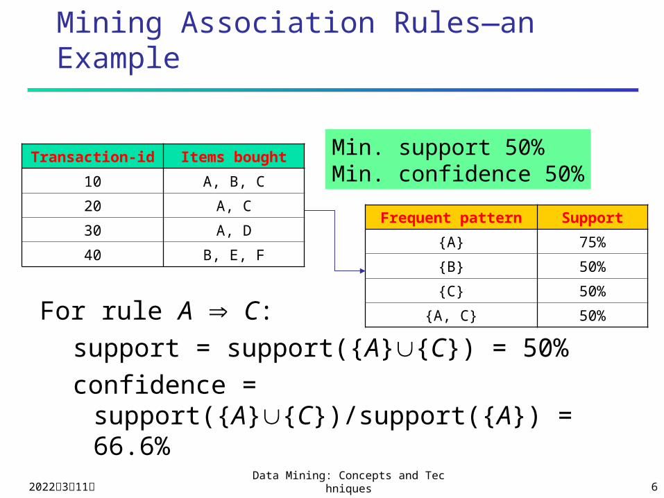
Mining Association Rules—an Example
For rule A C:support = support({A}{C}) = 50%confidence =
support({A}{C})/support({A}) = 66.6%
Min. support 50%Min. confidence 50%
Transaction-id Items bought
10 A, B, C
20 A, C
30 A, D
40 B, E, F
Frequent pattern Support
{A} 75%
{B} 50%
{C} 50%
{A, C} 50%

2023年4月19日Data Mining: Concepts and Technique
s 7
From Mining Association Rules to Mining Frequent Patterns (i.e. Frequent Itemsets)
Given a frequent itemset X, how to find association
rules?
Examine every subset S of X.
Confidence(S X – S ) = support(X)/support(S)
Compare with min_conf
An optimization is possible (refer to exercises
5.1, 5.2).
2023年4月19日Data Mining: Concepts and Technique
s 8
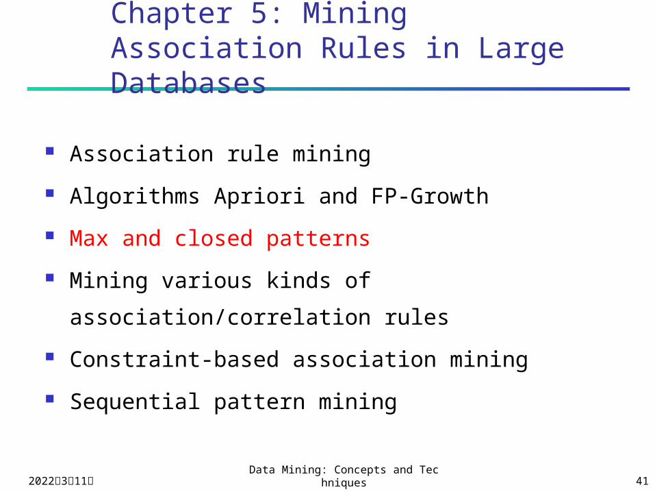
Chapter 5: Mining Association Rules in Large Databases
Association rule mining
Algorithms Apriori and FP-Growth
Max and closed patterns
Mining various kinds of association/correlation
rules
Constraint-based association mining
Sequential pattern mining
2023年4月19日Data Mining: Concepts and Technique
s 9
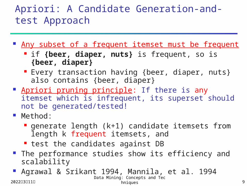
Apriori: A Candidate Generation-and-test Approach
Any subset of a frequent itemset must be frequent if {beer, diaper, nuts} is frequent, so is {beer,
diaper} Every transaction having {beer, diaper, nuts} also
contains {beer, diaper} Apriori pruning principle: If there is any itemset which is
infrequent, its superset should not be generated/tested! Method:
generate length (k+1) candidate itemsets from length k frequent itemsets, and
test the candidates against DB The performance studies show its efficiency and
scalability Agrawal & Srikant 1994, Mannila, et al. 1994
2023年4月19日Data Mining: Concepts and Technique
s 10
The Apriori Algorithm—An Example
Database TDB
1st scan
C1L1
L2
C2 C2
2nd scan
C3 L33rd scan
Tid Items
10 A, C, D
20 B, C, E
30 A, B, C, E
40 B, E
Itemset sup
{A} 2
{B} 3
{C} 3
{D} 1
{E} 3
Itemset sup
{A} 2
{B} 3
{C} 3
{E} 3
Itemset
{A, B}
{A, C}
{A, E}
{B, C}
{B, E}
{C, E}
Itemset sup{A, B} 1{A, C} 2{A, E} 1{B, C} 2{B, E} 3{C, E} 2
Itemset sup{A, C} 2{B, C} 2{B, E} 3{C, E} 2
Itemset
{B, C, E}Itemset sup{B, C, E} 2
2023年4月19日Data Mining: Concepts and Technique
s 11
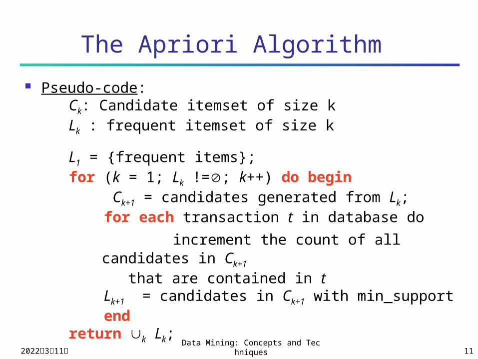
The Apriori Algorithm
Pseudo-code:Ck: Candidate itemset of size kLk : frequent itemset of size k
L1 = {frequent items};for (k = 1; Lk !=; k++) do begin Ck+1 = candidates generated from Lk; for each transaction t in database do
increment the count of all candidates in Ck+1 that are contained in t
Lk+1 = candidates in Ck+1 with min_support endreturn k Lk;
2023年4月19日Data Mining: Concepts and Technique
s 12
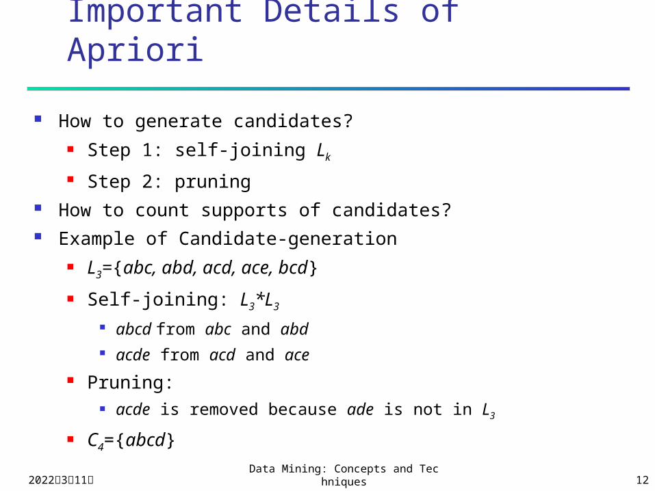
Important Details of Apriori
How to generate candidates? Step 1: self-joining Lk
Step 2: pruning How to count supports of candidates? Example of Candidate-generation
L3={abc, abd, acd, ace, bcd}
Self-joining: L3*L3
abcd from abc and abd acde from acd and ace
Pruning: acde is removed because ade is not in L3
C4={abcd}
2023年4月19日Data Mining: Concepts and Technique
s 13
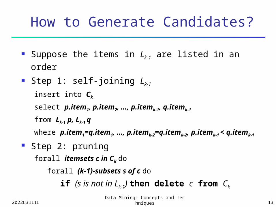
How to Generate Candidates?
Suppose the items in Lk-1 are listed in an order
Step 1: self-joining Lk-1
insert into Ck
select p.item1, p.item2, …, p.itemk-1, q.itemk-1
from Lk-1 p, Lk-1 q
where p.item1=q.item1, …, p.itemk-2=q.itemk-2, p.itemk-1
< q.itemk-1
Step 2: pruningforall itemsets c in Ck do
forall (k-1)-subsets s of c do
if (s is not in Lk-1) then delete c from Ck
2023年4月19日Data Mining: Concepts and Technique
s 14
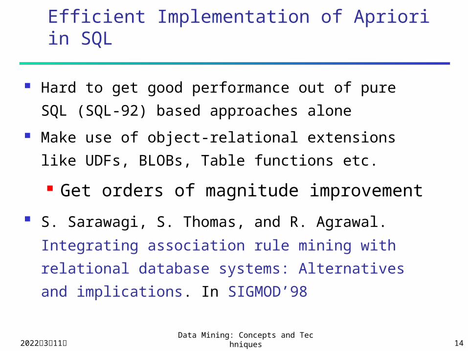
Efficient Implementation of Apriori in SQL
Hard to get good performance out of pure SQL
(SQL-92) based approaches alone
Make use of object-relational extensions like
UDFs, BLOBs, Table functions etc.
Get orders of magnitude improvement
S. Sarawagi, S. Thomas, and R. Agrawal. Integrating association rule mining with
relational database systems: Alternatives and
implications. In SIGMOD’98
2023年4月19日Data Mining: Concepts and Technique
s 15
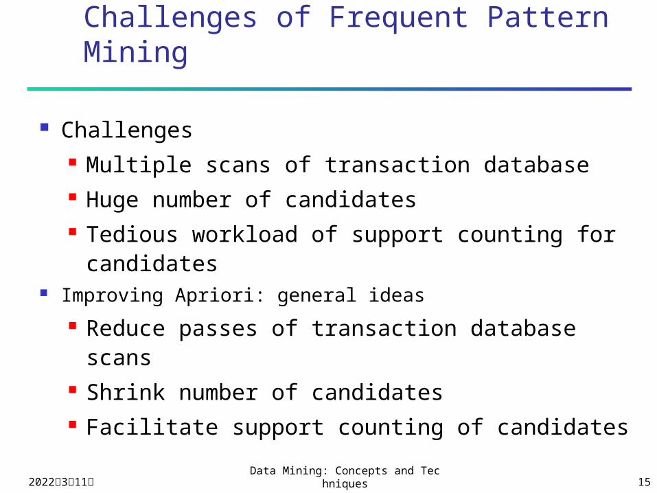
Challenges of Frequent Pattern Mining
Challenges Multiple scans of transaction database Huge number of candidates Tedious workload of support counting for
candidates Improving Apriori: general ideas
Reduce passes of transaction database scans
Shrink number of candidates Facilitate support counting of candidates
2023年4月19日Data Mining: Concepts and Technique
s 16
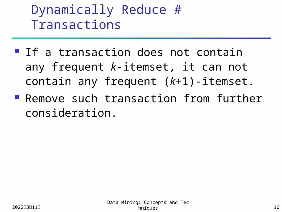
Dynamically Reduce # Transactions
If a transaction does not contain any frequent k-itemset, it can not contain any frequent (k+1)-itemset.
Remove such transaction from further consideration.
2023年4月19日Data Mining: Concepts and Technique
s 17
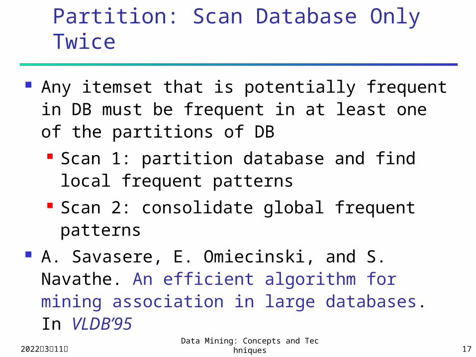
Partition: Scan Database Only Twice
Any itemset that is potentially frequent in DB must be frequent in at least one of the partitions of DB Scan 1: partition database and find local
frequent patterns Scan 2: consolidate global frequent
patterns A. Savasere, E. Omiecinski, and S. Navathe.
An efficient algorithm for mining association in large databases. In VLDB’95
2023年4月19日Data Mining: Concepts and Technique
s 18
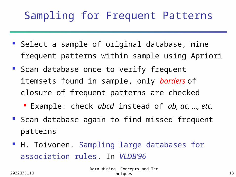
Sampling for Frequent Patterns
Select a sample of original database, mine
frequent patterns within sample using Apriori
Scan database once to verify frequent itemsets
found in sample, only borders of closure of
frequent patterns are checked
Example: check abcd instead of ab, ac, …, etc.
Scan database again to find missed frequent
patterns
H. Toivonen. Sampling large databases for
association rules. In VLDB’96
2023年4月19日Data Mining: Concepts and Technique
s 19
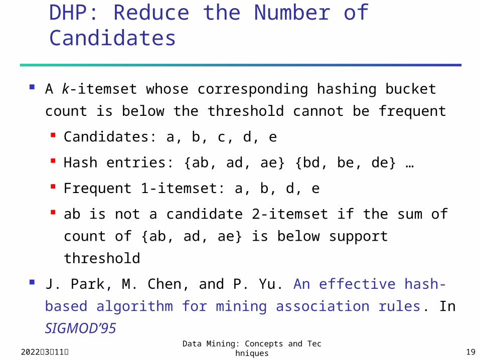
DHP: Reduce the Number of Candidates
A k-itemset whose corresponding hashing bucket
count is below the threshold cannot be frequent
Candidates: a, b, c, d, e
Hash entries: {ab, ad, ae} {bd, be, de} …
Frequent 1-itemset: a, b, d, e
ab is not a candidate 2-itemset if the sum of
count of {ab, ad, ae} is below support threshold
J. Park, M. Chen, and P. Yu. An effective hash-based
algorithm for mining association rules. In
SIGMOD’95
2023年4月19日Data Mining: Concepts and Technique
s 20
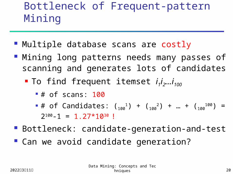
Bottleneck of Frequent-pattern Mining
Multiple database scans are costly Mining long patterns needs many passes of
scanning and generates lots of candidates To find frequent itemset i1i2…i100
# of scans: 100 # of Candidates: (100
1) + (1002) + … + (100
100) =
2100-1 = 1.27*1030 !
Bottleneck: candidate-generation-and-test Can we avoid candidate generation?
2023年4月19日Data Mining: Concepts and Technique
s 21
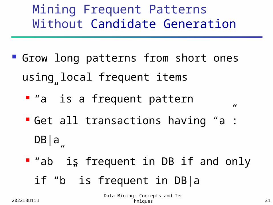
Mining Frequent Patterns Without Candidate Generation
Grow long patterns from short ones using
local frequent items
“a” is a frequent pattern
Get all transactions having “a”: DB|a
“ab” is frequent in DB if and only if “b” is
frequent in DB|a
2023年4月19日Data Mining: Concepts and Technique
s 22
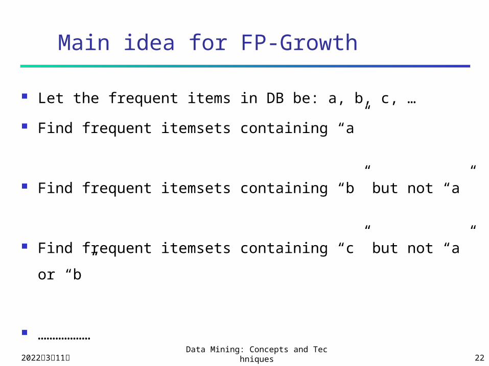
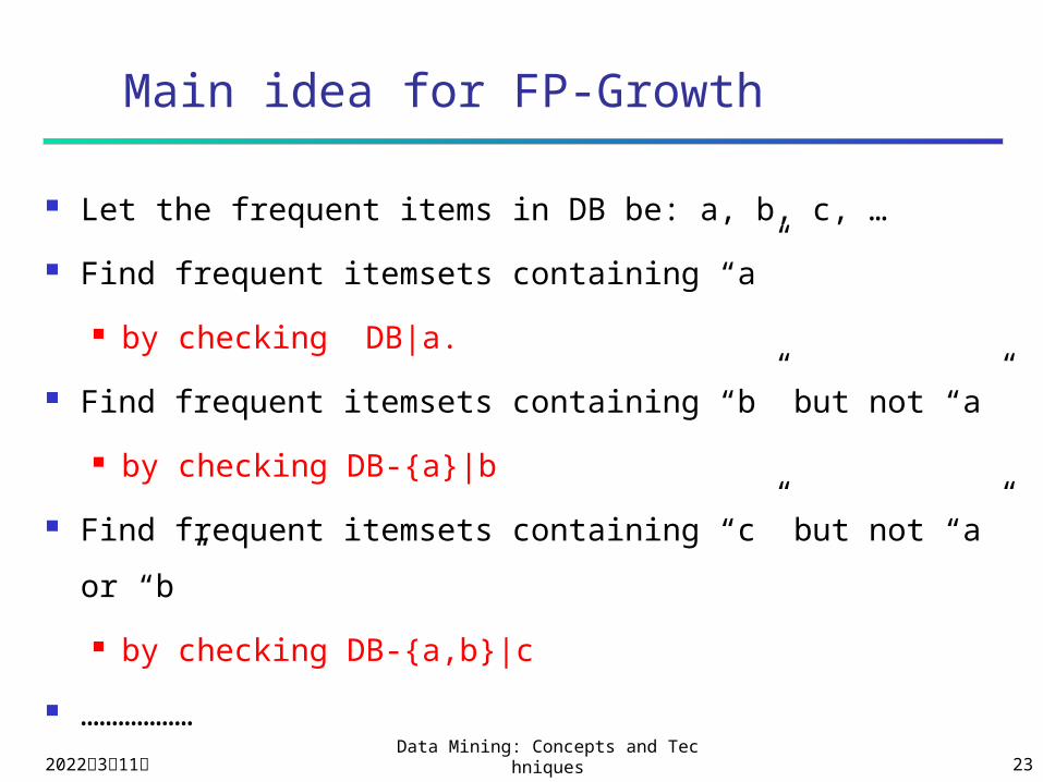
Main idea for FP-Growth
Let the frequent items in DB be: a, b, c, …
Find frequent itemsets containing “a”
Find frequent itemsets containing “b” but not “a”
Find frequent itemsets containing “c” but not “a” or “b”
………………
2023年4月19日Data Mining: Concepts and Technique
s 23
Main idea for FP-Growth
Let the frequent items in DB be: a, b, c, …
Find frequent itemsets containing “a”
by checking DB|a.
Find frequent itemsets containing “b” but not “a”
by checking DB-{a}|b
Find frequent itemsets containing “c” but not “a” or “b”
by checking DB-{a,b}|c
………………
2023年4月19日Data Mining: Concepts and Technique
s 24
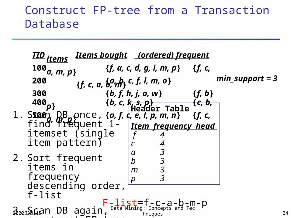
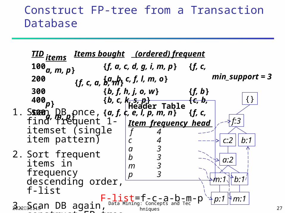
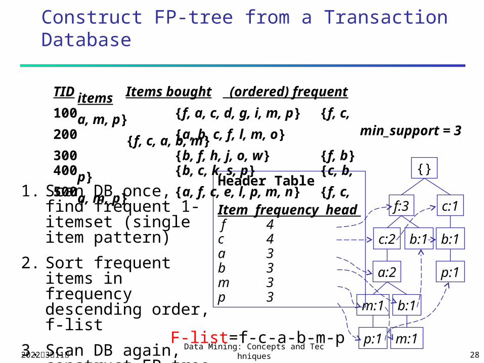
Construct FP-tree from a Transaction Database
Header Table
Item frequency head f 4c 4a 3b 3m 3p 3
min_support = 3
TID Items bought (ordered) frequent items100 {f, a, c, d, g, i, m, p} {f, c, a, m, p}200 {a, b, c, f, l, m, o} {f, c, a, b, m}300 {b, f, h, j, o, w} {f, b}400 {b, c, k, s, p} {c, b, p}500 {a, f, c, e, l, p, m, n} {f, c, a, m, p}
1. Scan DB once, find frequent 1-itemset (single item pattern)
2. Sort frequent items in frequency descending order, f-list
3. Scan DB again, construct FP-tree F-list=f-c-a-b-m-p
2023年4月19日Data Mining: Concepts and Technique
s 25
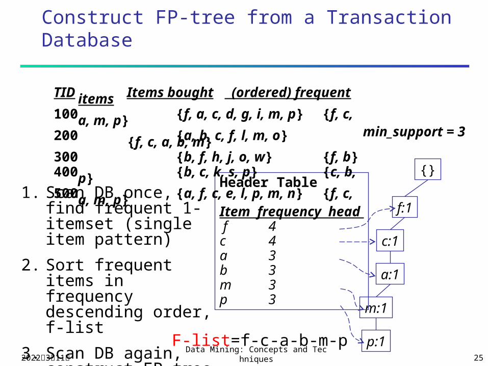
Construct FP-tree from a Transaction Database
{}
f:1
c:1
a:1
m:1
p:1
Header Table
Item frequency head f 4c 4a 3b 3m 3p 3
min_support = 3
TID Items bought (ordered) frequent items100 {f, a, c, d, g, i, m, p} {f, c, a, m, p}200 {a, b, c, f, l, m, o} {f, c, a, b, m}300 {b, f, h, j, o, w} {f, b}400 {b, c, k, s, p} {c, b, p}500 {a, f, c, e, l, p, m, n} {f, c, a, m, p}
1. Scan DB once, find frequent 1-itemset (single item pattern)
2. Sort frequent items in frequency descending order, f-list
3. Scan DB again, construct FP-tree F-list=f-c-a-b-m-p
2023年4月19日Data Mining: Concepts and Technique
s 26
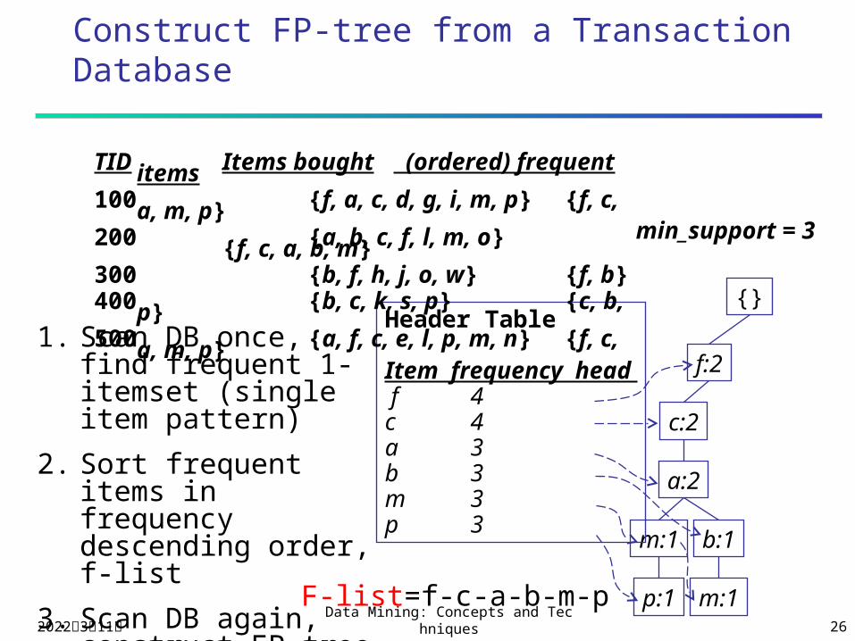
Construct FP-tree from a Transaction Database
{}
f:2
c:2
a:2
b:1m:1
p:1 m:1
Header Table
Item frequency head f 4c 4a 3b 3m 3p 3
min_support = 3
TID Items bought (ordered) frequent items100 {f, a, c, d, g, i, m, p} {f, c, a, m, p}200 {a, b, c, f, l, m, o} {f, c, a, b, m}300 {b, f, h, j, o, w} {f, b}400 {b, c, k, s, p} {c, b, p}500 {a, f, c, e, l, p, m, n} {f, c, a, m, p}
1. Scan DB once, find frequent 1-itemset (single item pattern)
2. Sort frequent items in frequency descending order, f-list
3. Scan DB again, construct FP-tree F-list=f-c-a-b-m-p
2023年4月19日Data Mining: Concepts and Technique
s 27
Construct FP-tree from a Transaction Database
{}
f:3
c:2
a:2
b:1m:1
p:1 m:1
Header Table
Item frequency head f 4c 4a 3b 3m 3p 3
min_support = 3
TID Items bought (ordered) frequent items100 {f, a, c, d, g, i, m, p} {f, c, a, m, p}200 {a, b, c, f, l, m, o} {f, c, a, b, m}300 {b, f, h, j, o, w} {f, b}400 {b, c, k, s, p} {c, b, p}500 {a, f, c, e, l, p, m, n} {f, c, a, m, p}
1. Scan DB once, find frequent 1-itemset (single item pattern)
2. Sort frequent items in frequency descending order, f-list
3. Scan DB again, construct FP-tree F-list=f-c-a-b-m-p
b:1
2023年4月19日Data Mining: Concepts and Technique
s 28
Construct FP-tree from a Transaction Database
{}
f:3 c:1
b:1
p:1
b:1c:2
a:2
b:1m:1
p:1 m:1
Header Table
Item frequency head f 4c 4a 3b 3m 3p 3
min_support = 3
TID Items bought (ordered) frequent items100 {f, a, c, d, g, i, m, p} {f, c, a, m, p}200 {a, b, c, f, l, m, o} {f, c, a, b, m}300 {b, f, h, j, o, w} {f, b}400 {b, c, k, s, p} {c, b, p}500 {a, f, c, e, l, p, m, n} {f, c, a, m, p}
1. Scan DB once, find frequent 1-itemset (single item pattern)
2. Sort frequent items in frequency descending order, f-list
3. Scan DB again, construct FP-tree F-list=f-c-a-b-m-p

2023年4月19日Data Mining: Concepts and Technique
s 29
Construct FP-tree from a Transaction Database
{}
f:4 c:1
b:1
p:1
b:1c:3
a:3
b:1m:2
p:2 m:1
Header Table
Item frequency head f 4c 4a 3b 3m 3p 3
min_support = 3
TID Items bought (ordered) frequent items100 {f, a, c, d, g, i, m, p} {f, c, a, m, p}200 {a, b, c, f, l, m, o} {f, c, a, b, m}300 {b, f, h, j, o, w} {f, b}400 {b, c, k, s, p} {c, b, p}500 {a, f, c, e, l, p, m, n} {f, c, a, m, p}
1. Scan DB once, find frequent 1-itemset (single item pattern)
2. Sort frequent items in frequency descending order, f-list
3. Scan DB again, construct FP-tree F-list=f-c-a-b-m-p
2023年4月19日Data Mining: Concepts and Technique
s 30
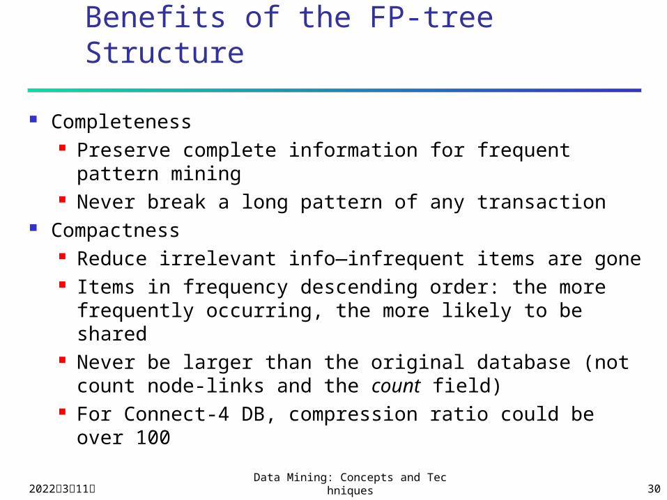
Benefits of the FP-tree Structure
Completeness Preserve complete information for frequent
pattern mining Never break a long pattern of any transaction
Compactness Reduce irrelevant info—infrequent items are gone Items in frequency descending order: the more
frequently occurring, the more likely to be shared Never be larger than the original database (not
count node-links and the count field) For Connect-4 DB, compression ratio could be
over 100
2023年4月19日Data Mining: Concepts and Technique
s 31
Partition Patterns and Databases
Frequent patterns can be partitioned into subsets according to f-list F-list=f-c-a-b-m-p Patterns containing p Patterns having m but no p … Patterns having c but no a nor b, m, p Pattern f
Completeness and non-redundency
2023年4月19日Data Mining: Concepts and Technique
s 32
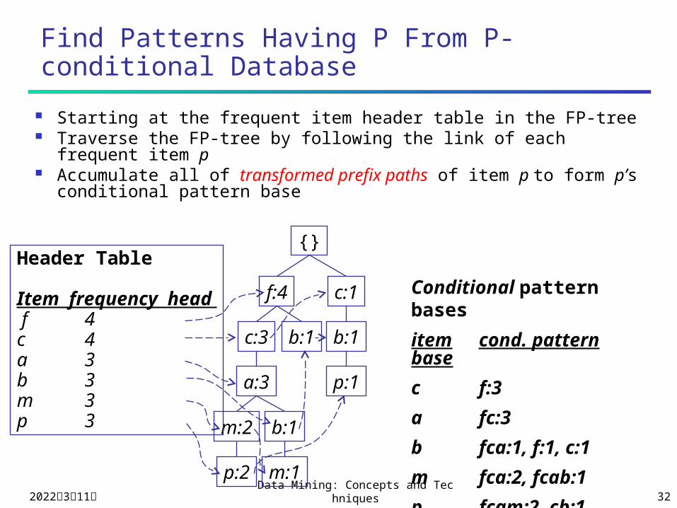
Find Patterns Having P From P-conditional Database
Starting at the frequent item header table in the FP-tree Traverse the FP-tree by following the link of each frequent
item p Accumulate all of transformed prefix paths of item p to
form p’s conditional pattern base
Conditional pattern bases
item cond. pattern base
c f:3
a fc:3
b fca:1, f:1, c:1
m fca:2, fcab:1
p fcam:2, cb:1
{}
f:4 c:1
b:1
p:1
b:1c:3
a:3
b:1m:2
p:2 m:1
Header Table
Item frequency head f 4c 4a 3b 3m 3p 3
2023年4月19日Data Mining: Concepts and Technique
s 33
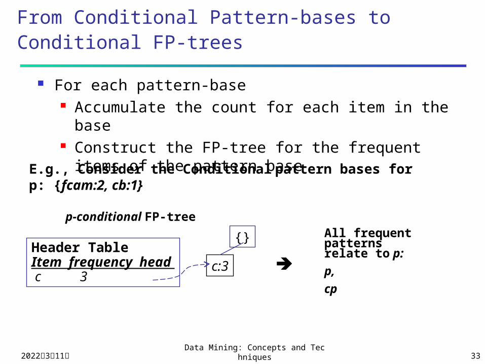
From Conditional Pattern-bases to Conditional FP-trees
For each pattern-base Accumulate the count for each item in the base Construct the FP-tree for the frequent items of
the pattern base
p-conditional FP-treeAll frequent patterns relate to p:
p,
cp
{}Header TableItem frequency head c 3
E.g., Consider the Conditional pattern bases for p: {fcam:2, cb:1}
c:3
2023年4月19日Data Mining: Concepts and Technique
s 34
From Conditional Pattern-bases to Conditional FP-trees
For each pattern-base Accumulate the count for each item in the base Construct the FP-tree for the frequent items of
the pattern base
m-conditional pattern base:fca:2, fcab:1
{}
f:3
c:3
a:3m-conditional FP-tree
All frequent patterns relate to m
m,
fm, cm, am,
fcm, fam, cam,
fcam
{}
f:4 c:1
b:1
p:1
b:1c:3
a:3
b:1m:2
p:2 m:1
Header TableItem frequency head f 4c 4a 3b 3m 3p 3
2023年4月19日Data Mining: Concepts and Technique
s 35
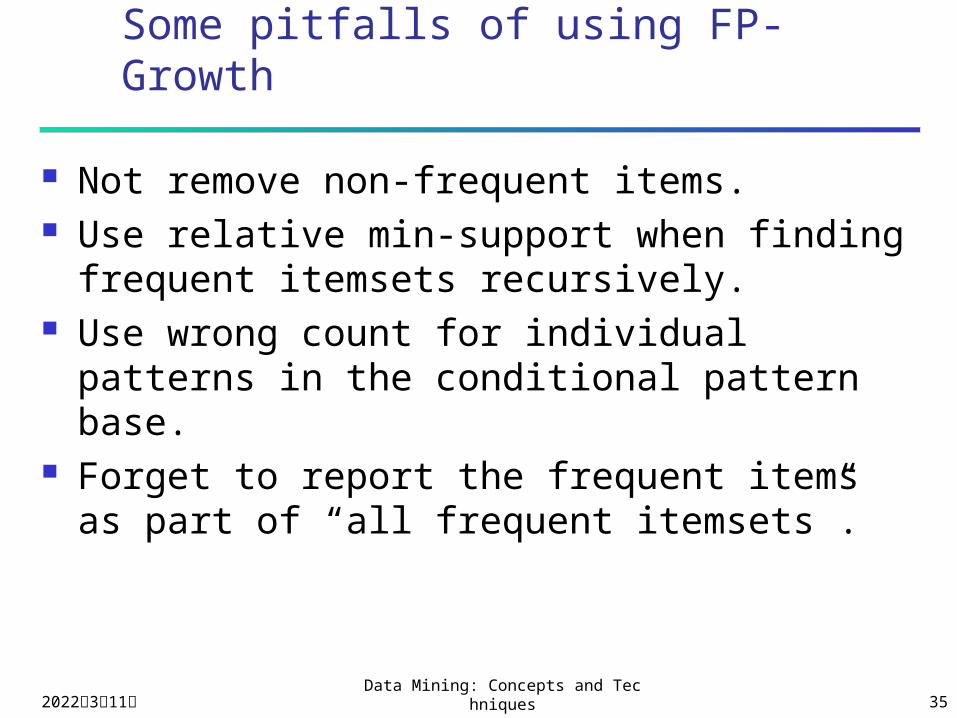
Some pitfalls of using FP-Growth
Not remove non-frequent items. Use relative min-support when finding
frequent itemsets recursively. Use wrong count for individual patterns in
the conditional pattern base. Forget to report the frequent items as part of
“all frequent itemsets”.
2023年4月19日Data Mining: Concepts and Technique
s 36
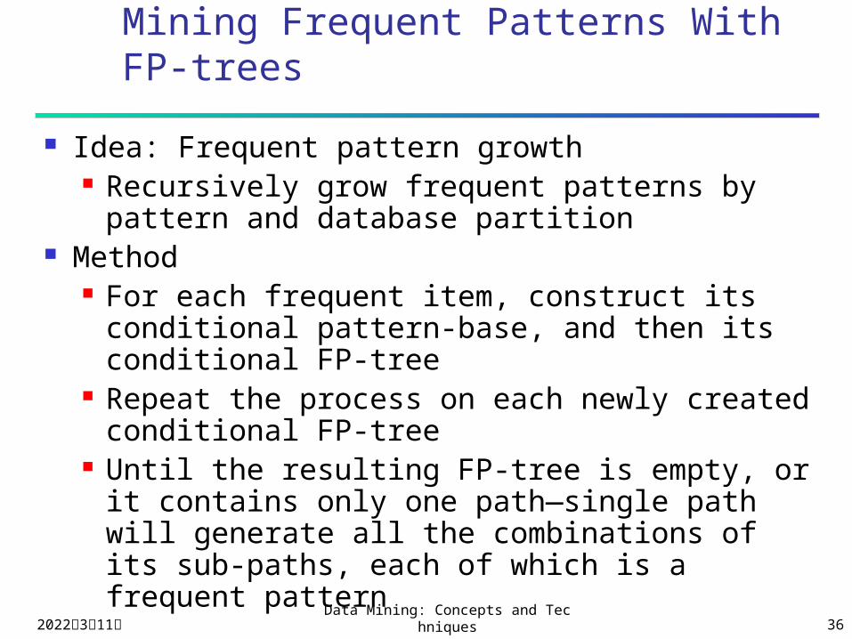
Mining Frequent Patterns With FP-trees
Idea: Frequent pattern growth Recursively grow frequent patterns by
pattern and database partition Method
For each frequent item, construct its conditional pattern-base, and then its conditional FP-tree
Repeat the process on each newly created conditional FP-tree
Until the resulting FP-tree is empty, or it contains only one path—single path will generate all the combinations of its sub-paths, each of which is a frequent pattern
2023年4月19日Data Mining: Concepts and Technique
s 37
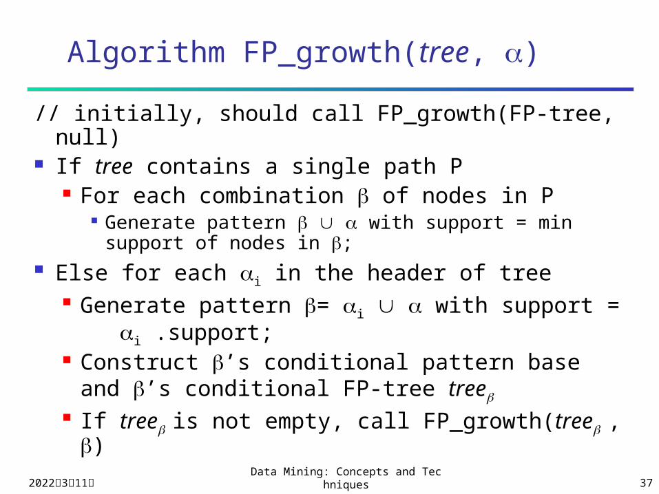
Algorithm FP_growth(tree, )
// initially, should call FP_growth(FP-tree, null) If tree contains a single path P
For each combination of nodes in P Generate pattern with support = min
support of nodes in ; Else for each i in the header of tree
Generate pattern = i with support = i .support;
Construct ’s conditional pattern base and ’s conditional FP-tree tree
If tree is not empty, call FP_growth(tree , )

2023年4月19日Data Mining: Concepts and Technique
s 38
A Special Case: Single Prefix Path in FP-tree
Suppose a (conditional) FP-tree T has a shared single prefix-path P
Mining can be decomposed into two parts Reduction of the single prefix path into one node Concatenation of the mining results of the two
parts
a2:n2
a3:n3
a1:n1
{}
b1:m1C1:k1
C2:k2 C3:k3
b1:m1C1:k1
C2:k2 C3:k3
r1
+a2:n2
a3:n3
a1:n1
{}
r1 =
2023年4月19日Data Mining: Concepts and Technique
s 39
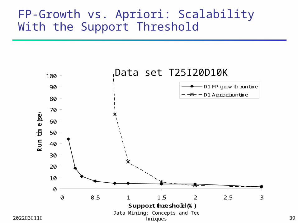
FP-Growth vs. Apriori: Scalability With the Support Threshold
0
10
20
30
40
50
60
70
80
90
100
0 0.5 1 1.5 2 2.5 3
Support threshold(%)
Ru
n t
ime
(se
c.)
D1 FP-grow th runtime
D1 Apriori runtime
Data set T25I20D10K
2023年4月19日Data Mining: Concepts and Technique
s 40
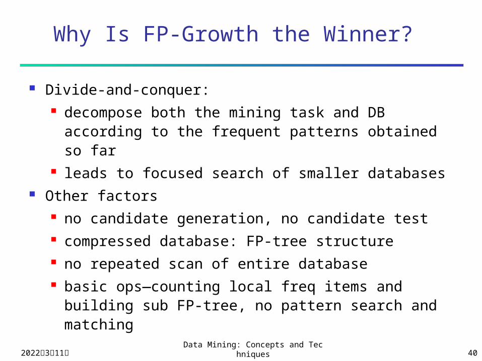
Why Is FP-Growth the Winner?
Divide-and-conquer: decompose both the mining task and DB
according to the frequent patterns obtained so far
leads to focused search of smaller databases Other factors
no candidate generation, no candidate test compressed database: FP-tree structure no repeated scan of entire database basic ops—counting local freq items and
building sub FP-tree, no pattern search and matching
2023年4月19日Data Mining: Concepts and Technique
s 41
Chapter 5: Mining Association Rules in Large Databases
Association rule mining
Algorithms Apriori and FP-Growth
Max and closed patterns
Mining various kinds of association/correlation
rules
Constraint-based association mining
Sequential pattern mining
2023年4月19日Data Mining: Concepts and Technique
s 42
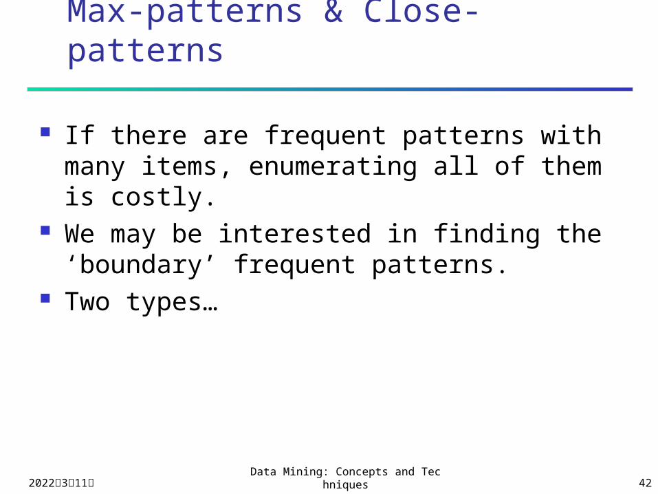
Max-patterns & Close-patterns
If there are frequent patterns with many items, enumerating all of them is costly.
We may be interested in finding the ‘boundary’ frequent patterns.
Two types…
2023年4月19日Data Mining: Concepts and Technique
s 43
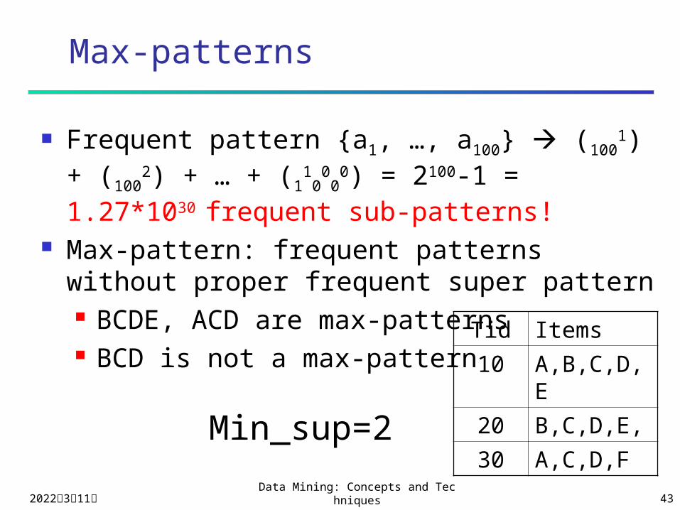
Max-patterns
Frequent pattern {a1, …, a100} (1001) +
(1002) + … + (1
10
00
0) = 2100-1 = 1.27*1030
frequent sub-patterns! Max-pattern: frequent patterns without
proper frequent super pattern BCDE, ACD are max-patterns BCD is not a max-pattern
Tid Items
10 A,B,C,D,E
20 B,C,D,E,
30 A,C,D,FMin_sup=2
2023年4月19日Data Mining: Concepts and Technique
s 44
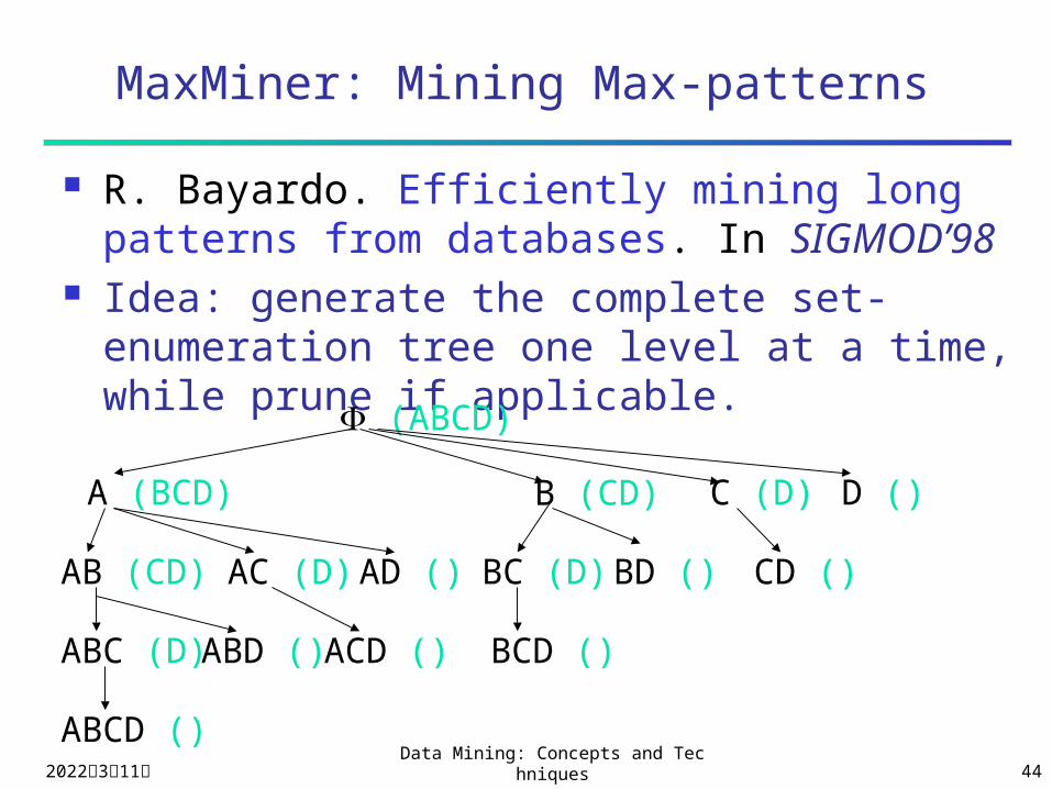
MaxMiner: Mining Max-patterns
R. Bayardo. Efficiently mining long patterns from databases. In SIGMOD’98
Idea: generate the complete set-enumeration tree one level at a time, while prune if applicable. (ABCD)
A (BCD) B (CD) C (D) D ()
AB (CD) AC (D) AD () BC (D) BD () CD ()
ABC (D)
ABCD ()
ABD () ACD () BCD ()
2023年4月19日Data Mining: Concepts and Technique
s 45
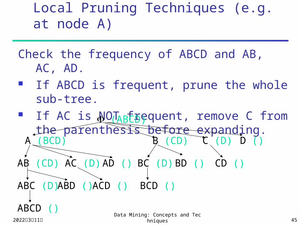
Local Pruning Techniques (e.g. at node A)
Check the frequency of ABCD and AB, AC, AD. If ABCD is frequent, prune the whole sub-
tree. If AC is NOT frequent, remove C from the
parenthesis before expanding. (ABCD)
A (BCD) B (CD) C (D) D ()
AB (CD) AC (D) AD () BC (D) BD () CD ()
ABC (D)
ABCD ()
ABD () ACD () BCD ()
2023年4月19日Data Mining: Concepts and Technique
s 46
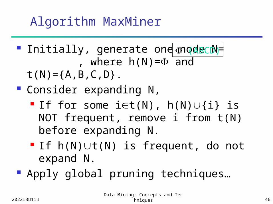
Algorithm MaxMiner
Initially, generate one node N= , where h(N)= and t(N)={A,B,C,D}.
Consider expanding N, If for some it(N), h(N){i} is NOT
frequent, remove i from t(N) before expanding N.
If h(N)t(N) is frequent, do not expand N. Apply global pruning techniques…
(ABCD)
2023年4月19日Data Mining: Concepts and Technique
s 47
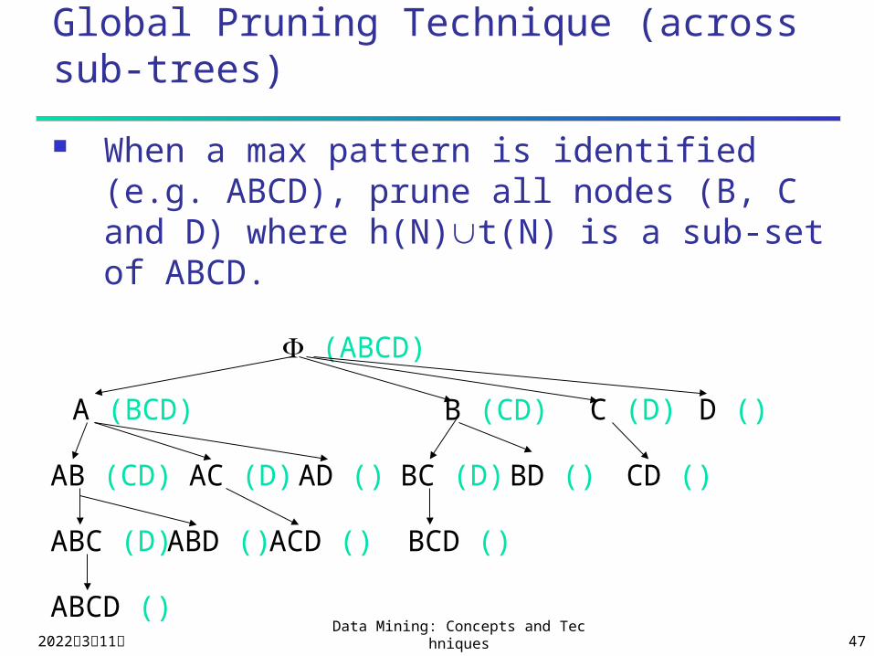
Global Pruning Technique (across sub-trees)
When a max pattern is identified (e.g. ABCD), prune all nodes (B, C and D) where h(N)t(N) is a sub-set of ABCD.
(ABCD)
A (BCD) B (CD) C (D) D ()
AB (CD) AC (D) AD () BC (D) BD () CD ()
ABC (D)
ABCD ()
ABD () ACD () BCD ()
2023年4月19日Data Mining: Concepts and Technique
s 48
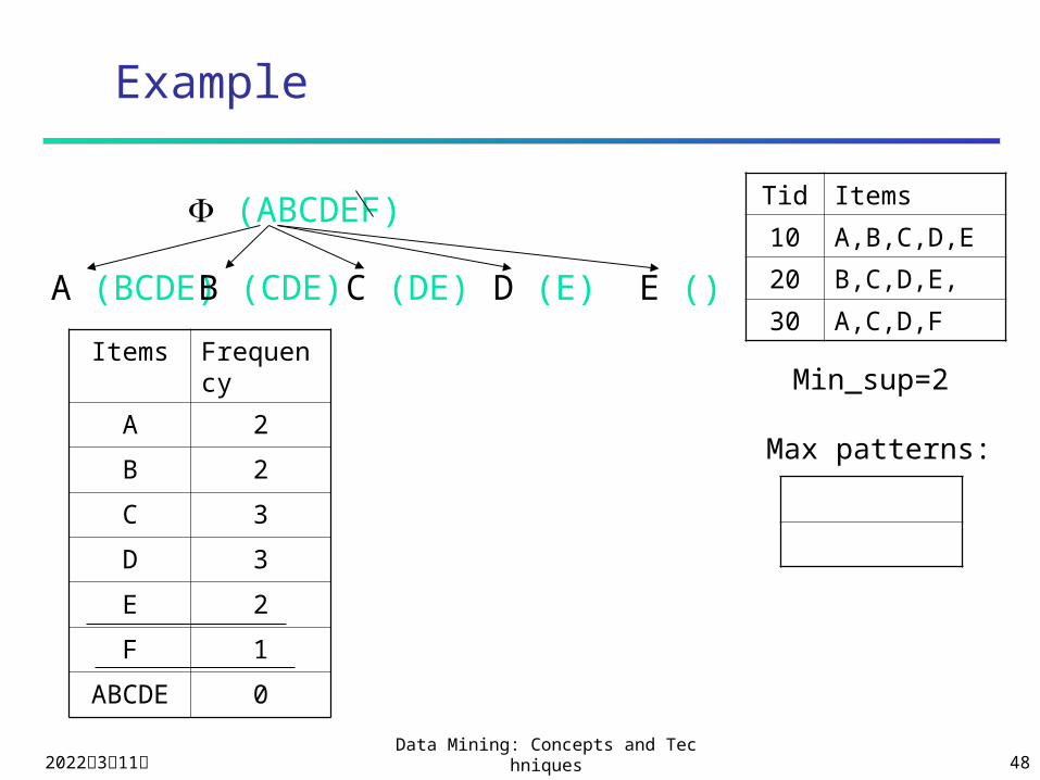
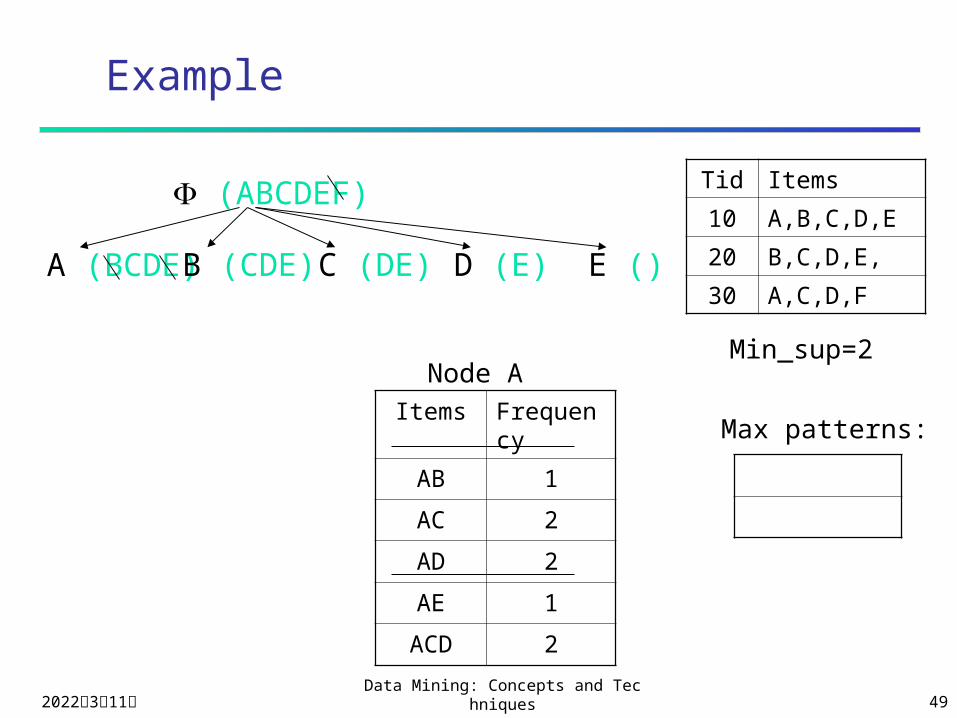
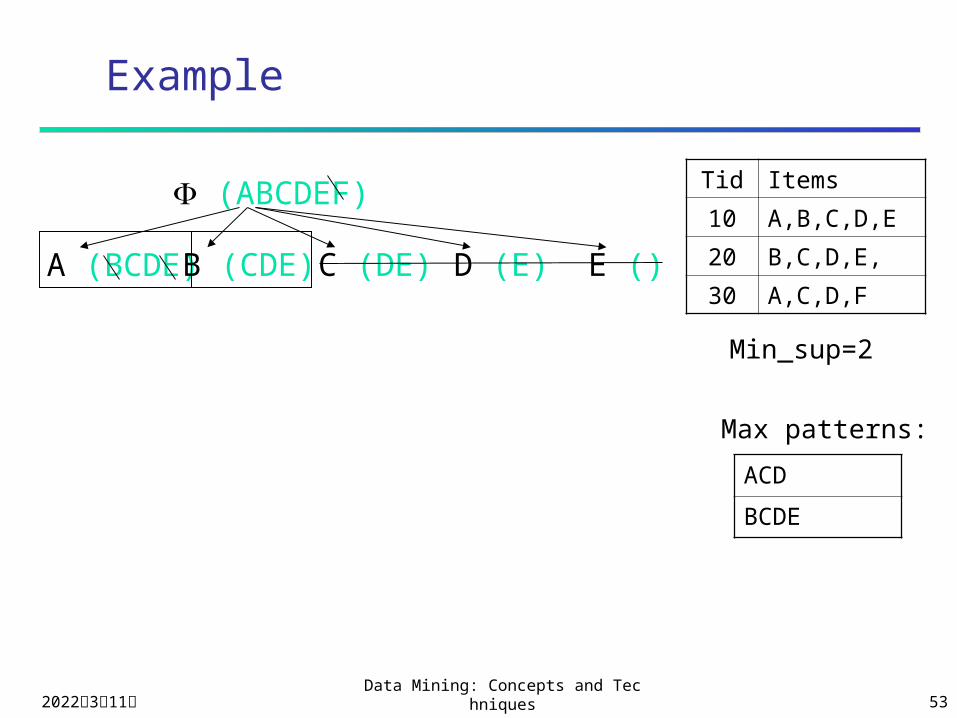
Example
Tid Items
10 A,B,C,D,E
20 B,C,D,E,
30 A,C,D,F
(ABCDEF)
Items Frequency
A 2
B 2
C 3
D 3
E 2
F 1
ABCDE 0
Min_sup=2
Max patterns:
A (BCDE)B (CDE) C (DE) E ()D (E)
2023年4月19日Data Mining: Concepts and Technique
s 49
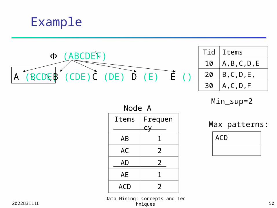
Example
Tid Items
10 A,B,C,D,E
20 B,C,D,E,
30 A,C,D,F
Items Frequency
AB 1
AC 2
AD 2
AE 1
ACD 2
Min_sup=2
(ABCDEF)
A (BCDE)B (CDE) C (DE) E ()D (E)
Max patterns:
Node A
2023年4月19日Data Mining: Concepts and Technique
s 50
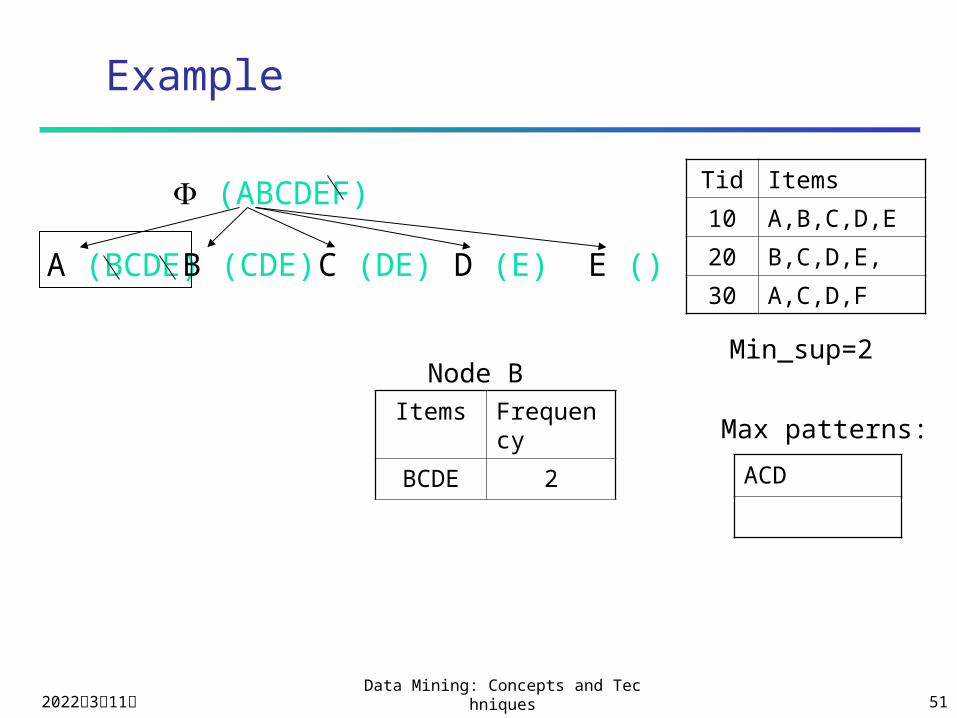
Example
Tid Items
10 A,B,C,D,E
20 B,C,D,E,
30 A,C,D,F
Items Frequency
AB 1
AC 2
AD 2
AE 1
ACD 2
Min_sup=2
(ABCDEF)
A (BCDE)B (CDE) C (DE) E ()D (E)
ACD
Max patterns:
Node A
2023年4月19日Data Mining: Concepts and Technique
s 51
Example
Tid Items
10 A,B,C,D,E
20 B,C,D,E,
30 A,C,D,F
Items Frequency
BCDE 2
Min_sup=2
(ABCDEF)
A (BCDE)B (CDE) C (DE) E ()D (E)
ACD
Max patterns:
Node B
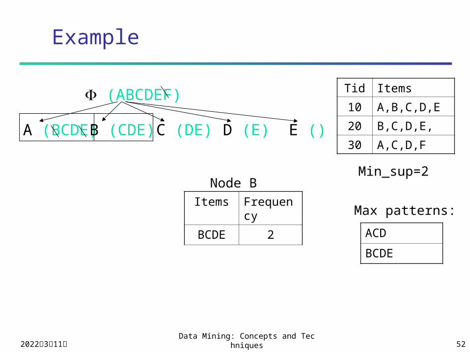
2023年4月19日Data Mining: Concepts and Technique
s 52
Example
Tid Items
10 A,B,C,D,E
20 B,C,D,E,
30 A,C,D,F
Items Frequency
BCDE 2
Min_sup=2
(ABCDEF)
A (BCDE)B (CDE) C (DE) E ()D (E)
ACD
BCDE
Max patterns:
Node B
2023年4月19日Data Mining: Concepts and Technique
s 53
Example
Tid Items
10 A,B,C,D,E
20 B,C,D,E,
30 A,C,D,F
Min_sup=2
(ABCDEF)
A (BCDE)B (CDE) C (DE) E ()D (E)
ACD
BCDE
Max patterns:
2023年4月19日Data Mining: Concepts and Technique
s 54
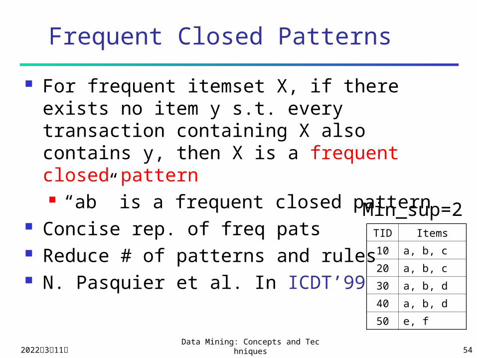
Frequent Closed Patterns
For frequent itemset X, if there exists no item y s.t. every transaction containing X also contains y, then X is a frequent closed pattern “ab” is a frequent closed pattern
Concise rep. of freq pats Reduce # of patterns and rules N. Pasquier et al. In ICDT’99
TID Items
10 a, b, c
20 a, b, c
30 a, b, d
40 a, b, d
50 e, f
Min_sup=2
2023年4月19日Data Mining: Concepts and Technique
s 55
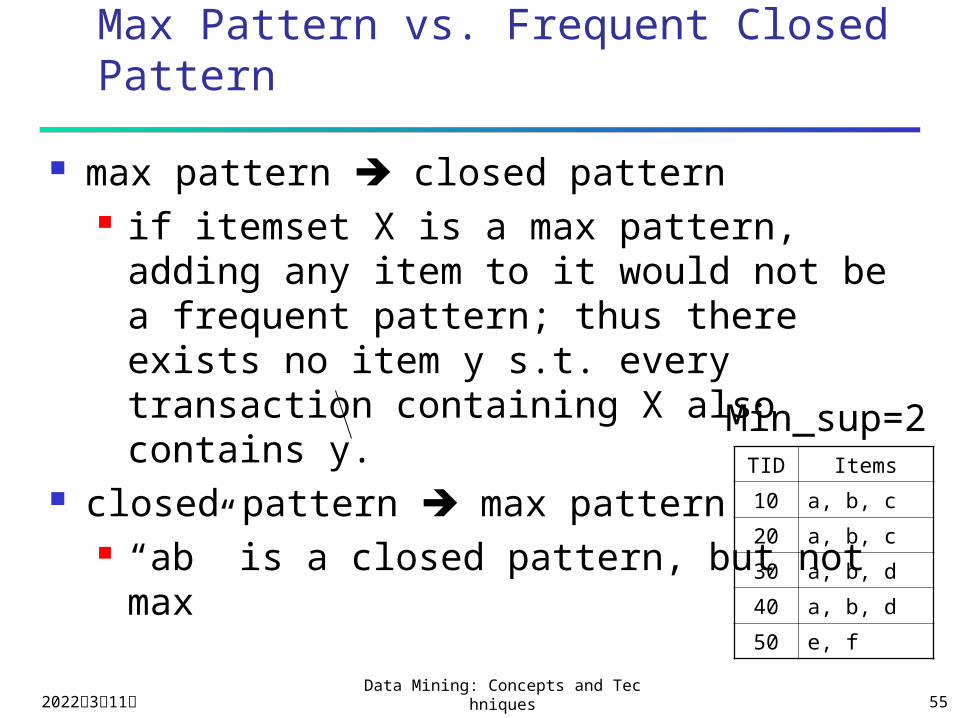
Max Pattern vs. Frequent Closed Pattern
max pattern closed pattern if itemset X is a max pattern, adding any
item to it would not be a frequent pattern; thus there exists no item y s.t. every transaction containing X also contains y.
closed pattern max pattern “ab” is a closed pattern, but not max
TID Items
10 a, b, c
20 a, b, c
30 a, b, d
40 a, b, d
50 e, f
Min_sup=2
2023年4月19日Data Mining: Concepts and Technique
s 56
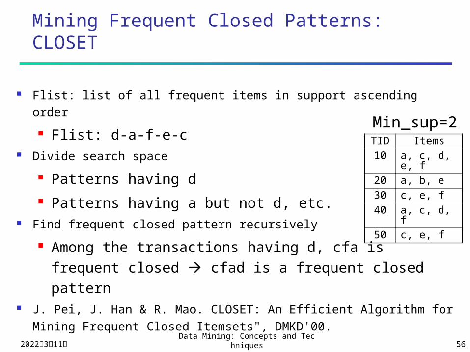
Mining Frequent Closed Patterns: CLOSET
Flist: list of all frequent items in support ascending order
Flist: d-a-f-e-c Divide search space
Patterns having d Patterns having a but not d, etc.
Find frequent closed pattern recursively
Among the transactions having d, cfa is frequent closed cfad is a frequent closed pattern
J. Pei, J. Han & R. Mao. CLOSET: An Efficient Algorithm for Mining Frequent Closed Itemsets", DMKD'00.
TID Items10 a, c, d, e, f20 a, b, e30 c, e, f40 a, c, d, f50 c, e, f
Min_sup=2
2023年4月19日Data Mining: Concepts and Technique
s 57
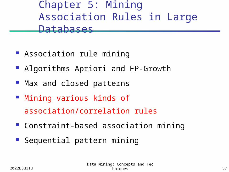
Chapter 5: Mining Association Rules in Large Databases
Association rule mining
Algorithms Apriori and FP-Growth
Max and closed patterns
Mining various kinds of association/correlation
rules
Constraint-based association mining
Sequential pattern mining

2023年4月19日Data Mining: Concepts and Technique
s 58
Mining Various Kinds of Rules or Regularities
Multi-level rules.
Multi-dimensional rules.
Correlation analysis.
2023年4月19日Data Mining: Concepts and Technique
s 59
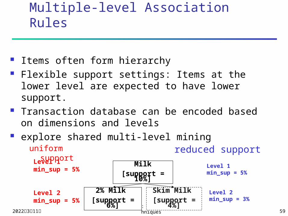
Multiple-level Association Rules
Items often form hierarchy Flexible support settings: Items at the lower level
are expected to have lower support. Transaction database can be encoded based on
dimensions and levels explore shared multi-level mining
uniform support
Milk[support = 10%]
2% Milk [support = 6%]
Skim Milk [support = 4%]
Level 1min_sup = 5%
Level 2min_sup = 5%
Level 1min_sup = 5%
Level 2min_sup = 3%
reduced support
2023年4月19日Data Mining: Concepts and Technique
s 60
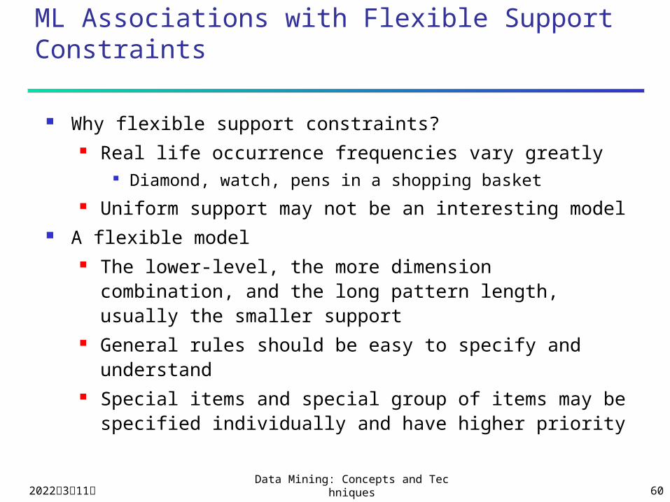
ML Associations with Flexible Support Constraints
Why flexible support constraints? Real life occurrence frequencies vary greatly
Diamond, watch, pens in a shopping basket Uniform support may not be an interesting model
A flexible model The lower-level, the more dimension combination, and
the long pattern length, usually the smaller support General rules should be easy to specify and understand Special items and special group of items may be
specified individually and have higher priority
2023年4月19日Data Mining: Concepts and Technique
s 61
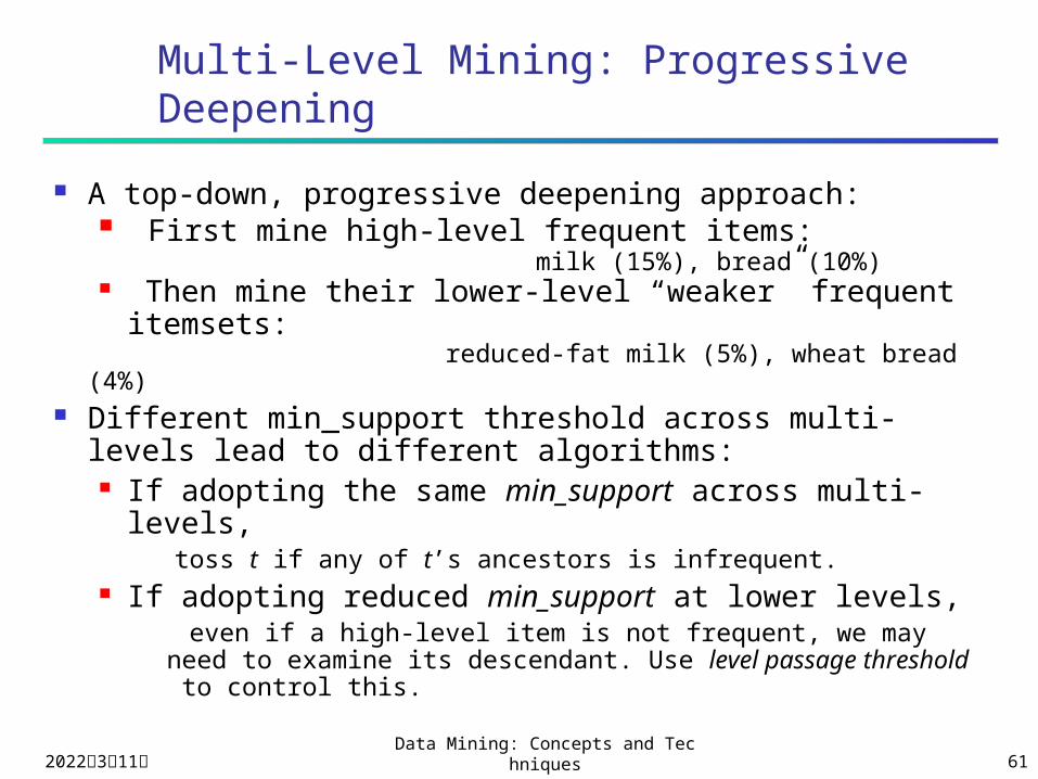
Multi-Level Mining: Progressive Deepening
A top-down, progressive deepening approach: First mine high-level frequent items:
milk (15%), bread (10%) Then mine their lower-level “weaker” frequent
itemsets: reduced-fat milk (5%), wheat bread (4%) Different min_support threshold across multi-levels
lead to different algorithms: If adopting the same min_support across multi-
levels, toss t if any of t’s ancestors is infrequent.
If adopting reduced min_support at lower levels, even if a high-level item is not frequent, we may need to
examine its descendant. Use level passage threshold to control this.
2023年4月19日Data Mining: Concepts and Technique
s 62
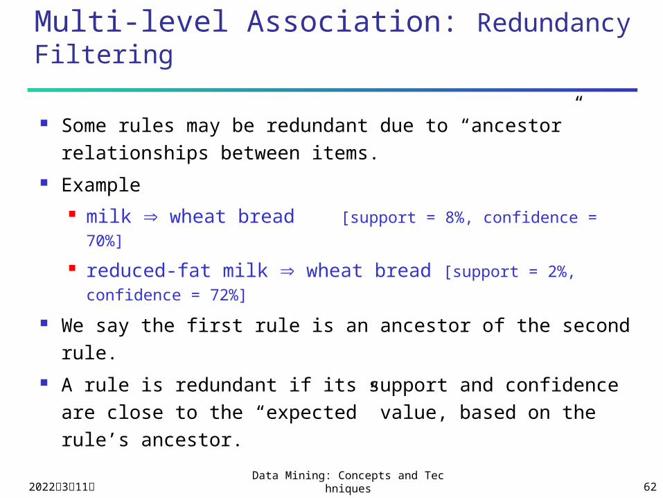
Multi-level Association: Redundancy Filtering
Some rules may be redundant due to “ancestor” relationships between items.
Example milk wheat bread [support = 8%, confidence = 70%]
reduced-fat milk wheat bread [support = 2%,
confidence = 72%]
We say the first rule is an ancestor of the second rule. A rule is redundant if its support and confidence are
close to the “expected” value, based on the rule’s ancestor.
2023年4月19日Data Mining: Concepts and Technique
s 63
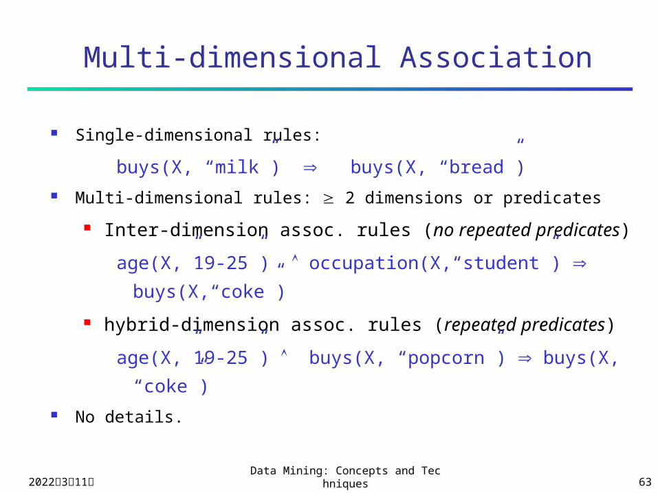
Multi-dimensional Association
Single-dimensional rules:
buys(X, “milk”) buys(X, “bread”) Multi-dimensional rules: 2 dimensions or predicates
Inter-dimension assoc. rules (no repeated predicates)
age(X,”19-25”) occupation(X,“student”)
buys(X,“coke”)
hybrid-dimension assoc. rules (repeated predicates)
age(X,”19-25”) buys(X, “popcorn”) buys(X, “coke”) No details.
2023年4月19日Data Mining: Concepts and Technique
s 64
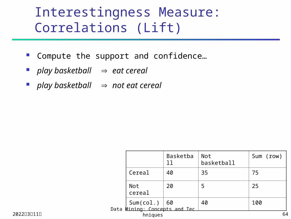
Interestingness Measure: Correlations (Lift)
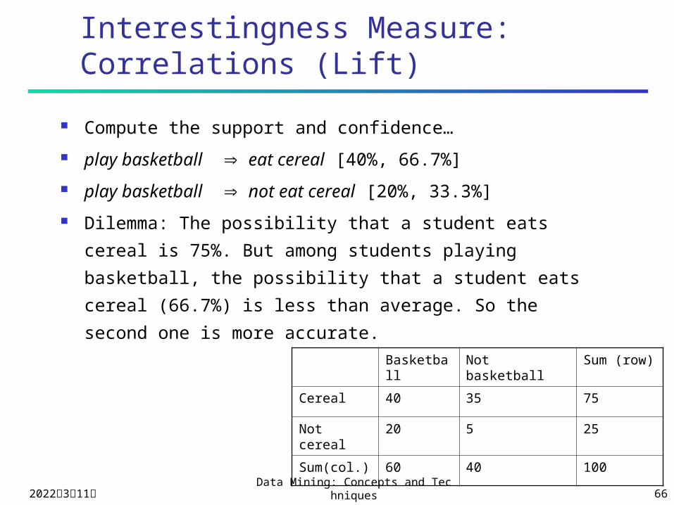
Compute the support and confidence…
play basketball eat cereal
play basketball not eat cereal
Basketball
Not basketball Sum (row)
Cereal 40 35 75
Not cereal 20 5 25
Sum(col.) 60 40 100
2023年4月19日Data Mining: Concepts and Technique
s 65
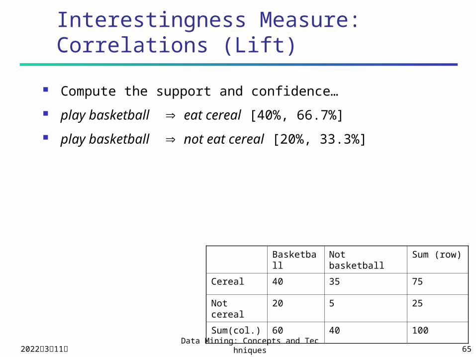
Interestingness Measure: Correlations (Lift)
Compute the support and confidence…
play basketball eat cereal [40%, 66.7%]
play basketball not eat cereal [20%, 33.3%]
Basketball
Not basketball Sum (row)
Cereal 40 35 75
Not cereal 20 5 25
Sum(col.) 60 40 100
2023年4月19日Data Mining: Concepts and Technique
s 66
Interestingness Measure: Correlations (Lift)
Compute the support and confidence…
play basketball eat cereal [40%, 66.7%]
play basketball not eat cereal [20%, 33.3%]
Dilemma: The possibility that a student eats cereal is
75%. But among students playing basketball, the
possibility that a student eats cereal (66.7%) is less
than average. So the second one is more accurate.
Basketball
Not basketball Sum (row)
Cereal 40 35 75
Not cereal 20 5 25
Sum(col.) 60 40 100
2023年4月19日Data Mining: Concepts and Technique
s 67
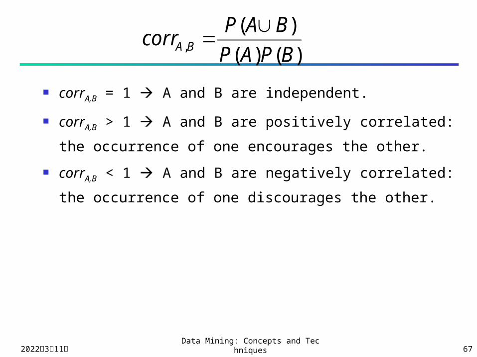
corrA,B = 1 A and B are independent.
corrA,B > 1 A and B are positively correlated: the
occurrence of one encourages the other.
corrA,B < 1 A and B are negatively correlated:
the occurrence of one discourages the other.
)()(
)(, BPAP
BAPcorr BA
2023年4月19日Data Mining: Concepts and Technique
s 68
)()(
)(, BPAP
BAPcorr BA
For instance, A=‘buy milk’, B=‘buy bread’.
Among 100 persons, 30 buys milk and 30 buys bread.
I.e. P(A)=P(B)=30.
If A and B are independent, there should have 9
person who buy both milk and bread. That is, among
those who buys milk, the possibility that someone
buys bread remains 30%.
Here, P(AB)=P(A)*P(B|A) is the possibility that a
person buys both milk and bread.
If there are 20 persons who buy both milk and bread,
i.e. corrA,B > 1, the occurrence of one encourages the
other.
2023年4月19日Data Mining: Concepts and Technique
s 69
Chapter 5: Mining Association Rules in Large Databases
Association rule mining
Algorithms Apriori and FP-Growth
Max and closed patterns
Mining various kinds of association/correlation
rules
Constraint-based association mining
Sequential pattern mining

2023年4月19日Data Mining: Concepts and Technique
s 70
Constraint-based Data Mining
Finding all the patterns in a database autonomously? — unrealistic! The patterns could be too many but not focused!
Data mining should be an interactive process User directs what to be mined using a data mining
query language (or a graphical user interface) Constraint-based mining
User flexibility: provides constraints on what to be mined
System optimization: explores such constraints for efficient mining—constraint-based mining
2023年4月19日Data Mining: Concepts and Technique
s 71
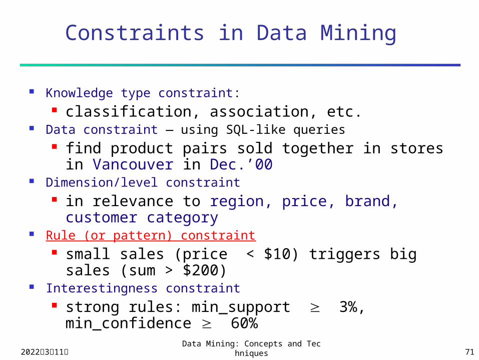
Constraints in Data Mining
Knowledge type constraint: classification, association, etc.
Data constraint — using SQL-like queries find product pairs sold together in stores in
Vancouver in Dec.’00 Dimension/level constraint
in relevance to region, price, brand, customer category
Rule (or pattern) constraint small sales (price < $10) triggers big sales (sum
> $200) Interestingness constraint
strong rules: min_support 3%, min_confidence 60%
2023年4月19日Data Mining: Concepts and Technique
s 72
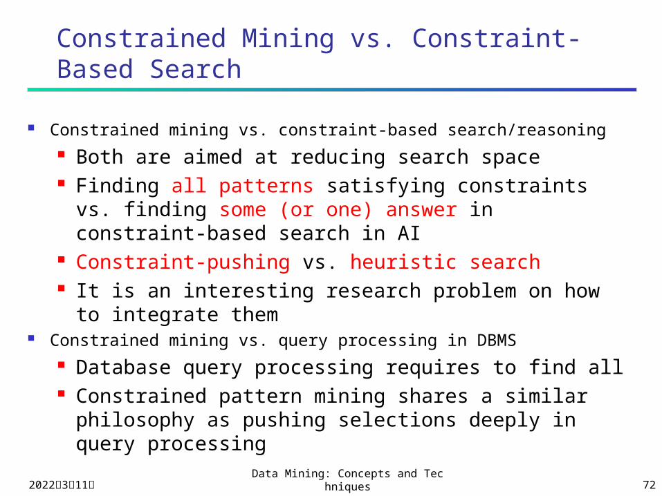
Constrained Mining vs. Constraint-Based Search
Constrained mining vs. constraint-based search/reasoning Both are aimed at reducing search space Finding all patterns satisfying constraints vs. finding
some (or one) answer in constraint-based search in AI
Constraint-pushing vs. heuristic search It is an interesting research problem on how to
integrate them Constrained mining vs. query processing in DBMS
Database query processing requires to find all Constrained pattern mining shares a similar
philosophy as pushing selections deeply in query processing
2023年4月19日Data Mining: Concepts and Technique
s 73
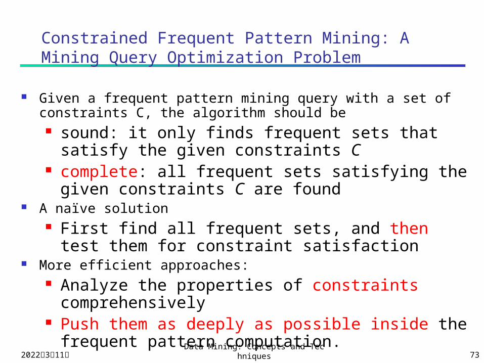
Constrained Frequent Pattern Mining: A Mining Query Optimization Problem
Given a frequent pattern mining query with a set of constraints C, the algorithm should be sound: it only finds frequent sets that satisfy the
given constraints C complete: all frequent sets satisfying the given
constraints C are found A naïve solution
First find all frequent sets, and then test them for constraint satisfaction
More efficient approaches: Analyze the properties of constraints
comprehensively Push them as deeply as possible inside the
frequent pattern computation.
2023年4月19日Data Mining: Concepts and Technique
s 74
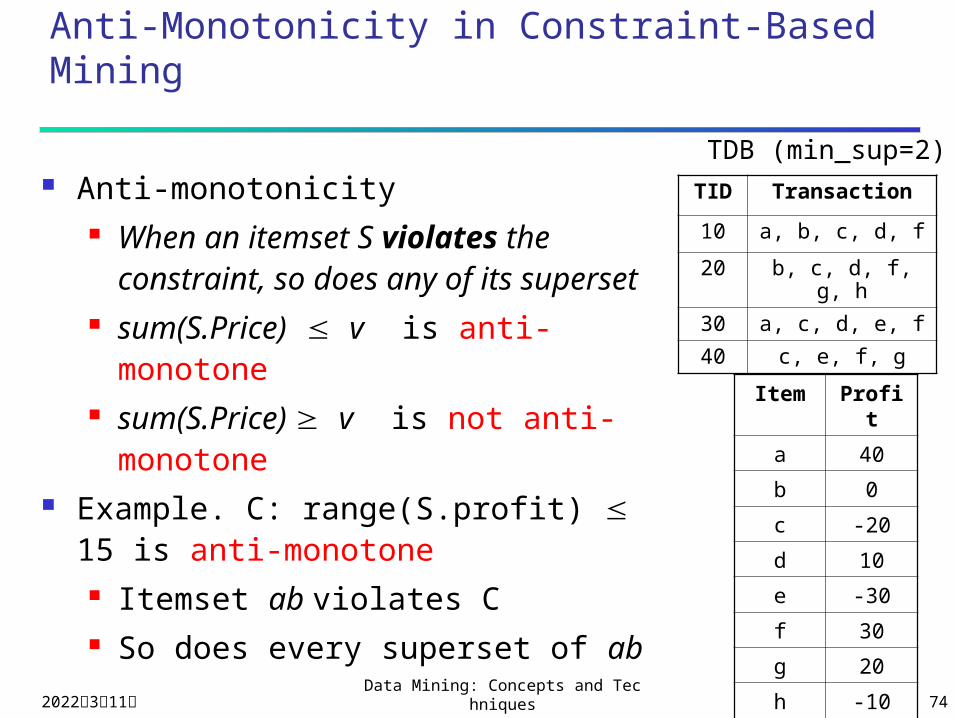
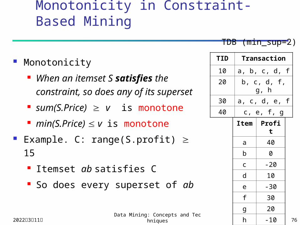
Anti-Monotonicity in Constraint-Based Mining
Anti-monotonicity When an itemset S violates the
constraint, so does any of its superset
sum(S.Price) v is anti-monotone sum(S.Price) v is not anti-
monotone Example. C: range(S.profit) 15 is
anti-monotone Itemset ab violates C So does every superset of ab
TID Transaction
10 a, b, c, d, f
20 b, c, d, f, g, h
30 a, c, d, e, f
40 c, e, f, g
TDB (min_sup=2)
Item Profit
a 40
b 0
c -20
d 10
e -30
f 30
g 20
h -10
2023年4月19日Data Mining: Concepts and Technique
s 75
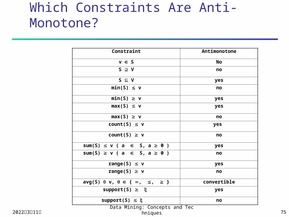
Which Constraints Are Anti-Monotone?
Constraint Antimonotone
v S No
S V no
S V yes
min(S) v no
min(S) v yes
max(S) v yes
max(S) v no
count(S) v yes
count(S) v no
sum(S) v ( a S, a 0 ) yes
sum(S) v ( a S, a 0 ) no
range(S) v yes
range(S) v no
avg(S) v, { , , } convertible
support(S) yes
support(S) no
2023年4月19日Data Mining: Concepts and Technique
s 76
Monotonicity in Constraint-Based Mining
Monotonicity When an itemset S satisfies
the constraint, so does any of its superset
sum(S.Price) v is monotone min(S.Price) v is monotone
Example. C: range(S.profit) 15 Itemset ab satisfies C So does every superset of ab
TID Transaction
10 a, b, c, d, f
20 b, c, d, f, g, h
30 a, c, d, e, f
40 c, e, f, g
TDB (min_sup=2)
Item Profit
a 40
b 0
c -20
d 10
e -30
f 30
g 20
h -10
2023年4月19日Data Mining: Concepts and Technique
s 77
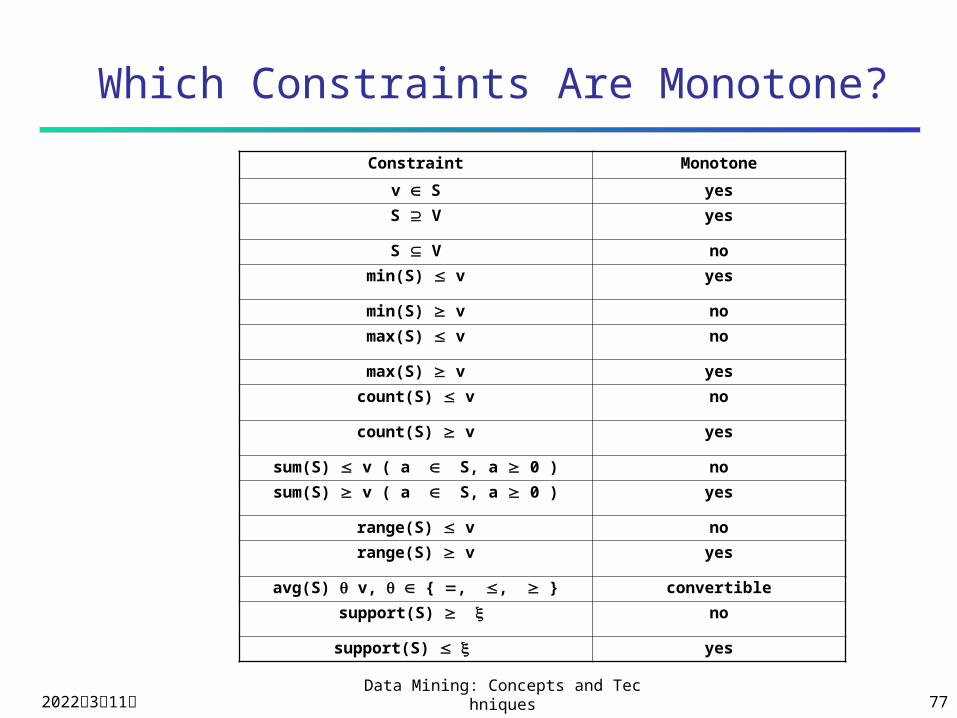
Which Constraints Are Monotone?
Constraint Monotone
v S yes
S V yes
S V no
min(S) v yes
min(S) v no
max(S) v no
max(S) v yes
count(S) v no
count(S) v yes
sum(S) v ( a S, a 0 ) no
sum(S) v ( a S, a 0 ) yes
range(S) v no
range(S) v yes
avg(S) v, { , , } convertible
support(S) no
support(S) yes
2023年4月19日Data Mining: Concepts and Technique
s 78
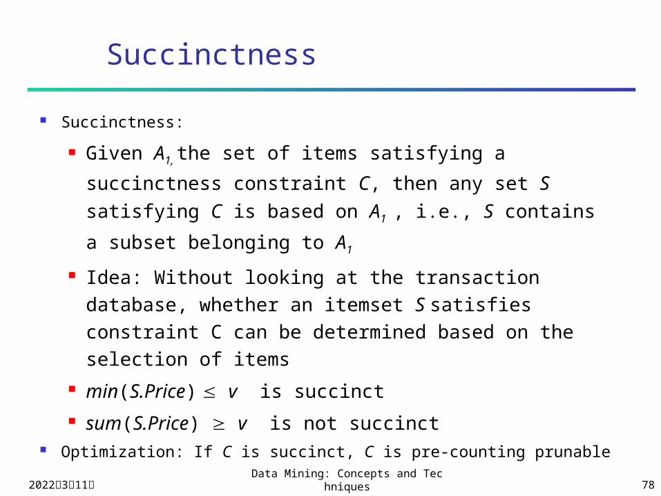
Succinctness
Succinctness:
Given A1, the set of items satisfying a
succinctness constraint C, then any set S
satisfying C is based on A1 , i.e., S contains a
subset belonging to A1
Idea: Without looking at the transaction database, whether an itemset S satisfies constraint C can be determined based on the selection of items
min(S.Price) v is succinct sum(S.Price) v is not succinct
Optimization: If C is succinct, C is pre-counting prunable
2023年4月19日Data Mining: Concepts and Technique
s 79
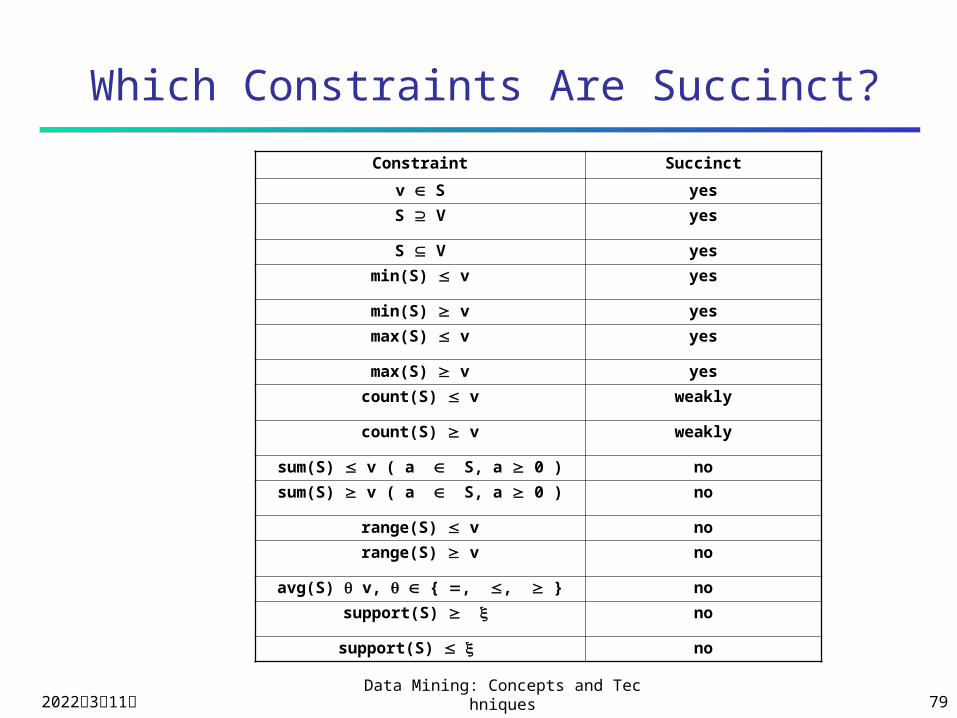
Which Constraints Are Succinct?
Constraint Succinct
v S yes
S V yes
S V yes
min(S) v yes
min(S) v yes
max(S) v yes
max(S) v yes
count(S) v weakly
count(S) v weakly
sum(S) v ( a S, a 0 ) no
sum(S) v ( a S, a 0 ) no
range(S) v no
range(S) v no
avg(S) v, { , , } no
support(S) no
support(S) no
2023年4月19日Data Mining: Concepts and Technique
s 80
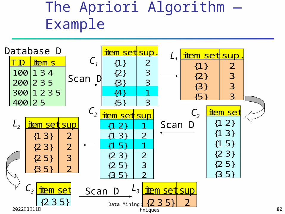
The Apriori Algorithm — Example
TID Items100 1 3 4200 2 3 5300 1 2 3 5400 2 5
Database D itemset sup.{1} 2{2} 3{3} 3{4} 1{5} 3
itemset sup.{1} 2{2} 3{3} 3{5} 3
Scan D
C1L1
itemset{1 2}{1 3}{1 5}{2 3}{2 5}{3 5}
itemset sup{1 2} 1{1 3} 2{1 5} 1{2 3} 2{2 5} 3{3 5} 2
itemset sup{1 3} 2{2 3} 2{2 5} 3{3 5} 2
L2
C2 C2
Scan D
C3 L3itemset{2 3 5}
Scan D itemset sup{2 3 5} 2
2023年4月19日Data Mining: Concepts and Technique
s 81
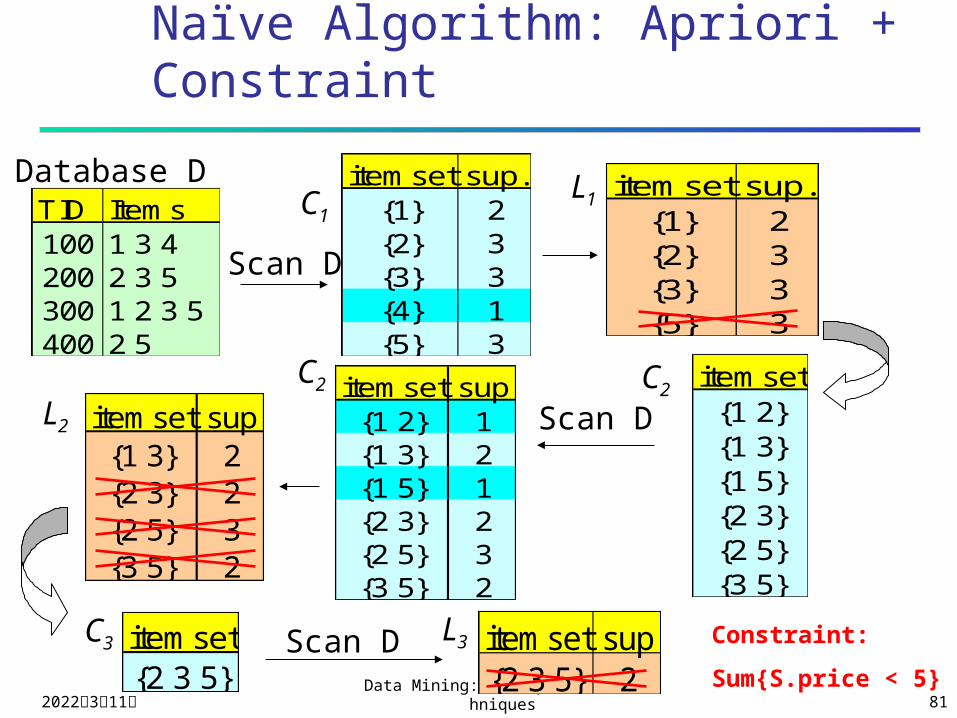
Naïve Algorithm: Apriori + Constraint
TID Items100 1 3 4200 2 3 5300 1 2 3 5400 2 5
Database D itemset sup.{1} 2{2} 3{3} 3{4} 1{5} 3
itemset sup.{1} 2{2} 3{3} 3{5} 3
Scan D
C1L1
itemset{1 2}{1 3}{1 5}{2 3}{2 5}{3 5}
itemset sup{1 2} 1{1 3} 2{1 5} 1{2 3} 2{2 5} 3{3 5} 2
itemset sup{1 3} 2{2 3} 2{2 5} 3{3 5} 2
L2
C2 C2
Scan D
C3 L3itemset{2 3 5}
Scan D itemset sup{2 3 5} 2
Constraint:
Sum{S.price < 5}
2023年4月19日Data Mining: Concepts and Technique
s 82
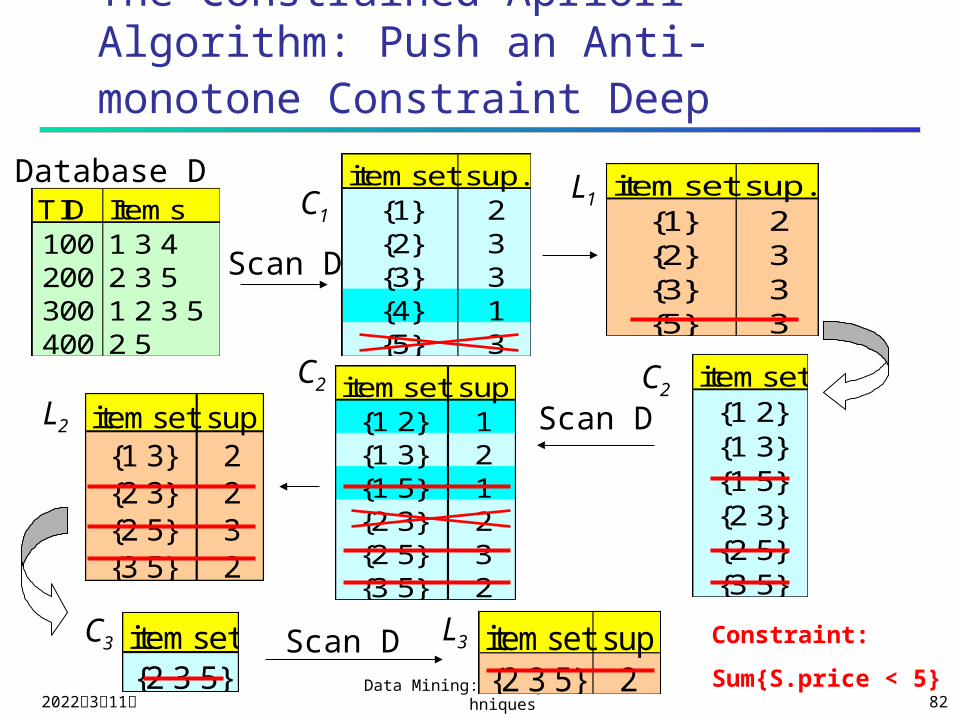
The Constrained Apriori Algorithm: Push an Anti-monotone Constraint Deep
TID Items100 1 3 4200 2 3 5300 1 2 3 5400 2 5
Database D itemset sup.{1} 2{2} 3{3} 3{4} 1{5} 3
itemset sup.{1} 2{2} 3{3} 3{5} 3
Scan D
C1L1
itemset{1 2}{1 3}{1 5}{2 3}{2 5}{3 5}
itemset sup{1 2} 1{1 3} 2{1 5} 1{2 3} 2{2 5} 3{3 5} 2
itemset sup{1 3} 2{2 3} 2{2 5} 3{3 5} 2
L2
C2 C2
Scan D
C3 L3itemset{2 3 5}
Scan D itemset sup{2 3 5} 2
Constraint:
Sum{S.price < 5}
2023年4月19日Data Mining: Concepts and Technique
s 83
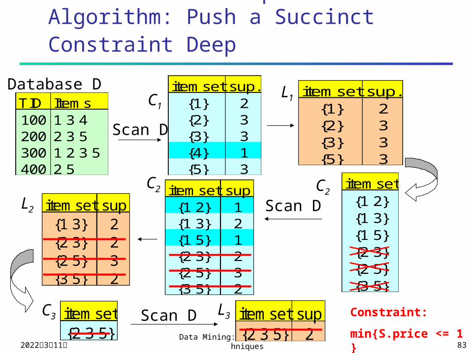
The Constrained Apriori Algorithm: Push a Succinct Constraint Deep
TID Items100 1 3 4200 2 3 5300 1 2 3 5400 2 5
Database D itemset sup.{1} 2{2} 3{3} 3{4} 1{5} 3
itemset sup.{1} 2{2} 3{3} 3{5} 3
Scan D
C1L1
itemset{1 2}{1 3}{1 5}{2 3}{2 5}{3 5}
itemset sup{1 2} 1{1 3} 2{1 5} 1{2 3} 2{2 5} 3{3 5} 2
itemset sup{1 3} 2{2 3} 2{2 5} 3{3 5} 2
L2
C2 C2
Scan D
C3 L3itemset{2 3 5}
Scan D itemset sup{2 3 5} 2
Constraint:
min{S.price <= 1 }
2023年4月19日Data Mining: Concepts and Technique
s 84
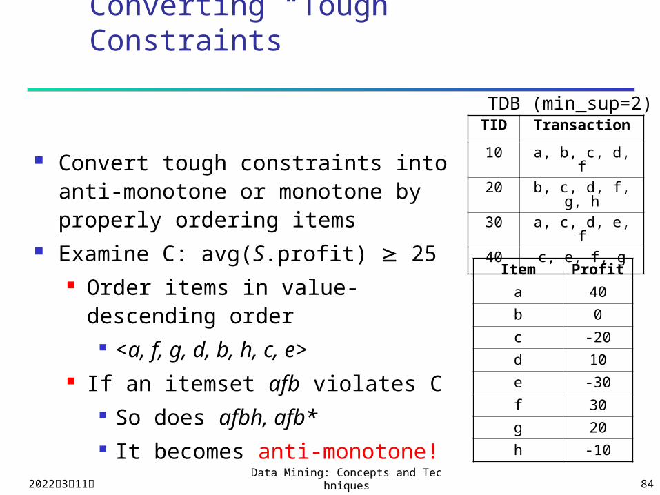
Converting “Tough” Constraints
Convert tough constraints into anti-monotone or monotone by properly ordering items
Examine C: avg(S.profit) 25 Order items in value-descending
order <a, f, g, d, b, h, c, e>
If an itemset afb violates C So does afbh, afb* It becomes anti-monotone!
TID Transaction
10 a, b, c, d, f
20 b, c, d, f, g, h
30 a, c, d, e, f
40 c, e, f, g
TDB (min_sup=2)
Item Profit
a 40
b 0
c -20
d 10
e -30
f 30
g 20
h -10
2023年4月19日Data Mining: Concepts and Technique
s 85
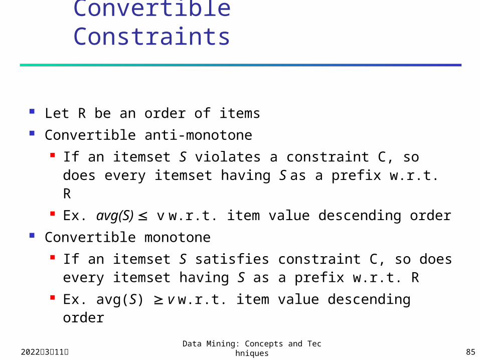
Convertible Constraints
Let R be an order of items Convertible anti-monotone
If an itemset S violates a constraint C, so does every itemset having S as a prefix w.r.t. R
Ex. avg(S) v w.r.t. item value descending order Convertible monotone
If an itemset S satisfies constraint C, so does every itemset having S as a prefix w.r.t. R
Ex. avg(S) v w.r.t. item value descending order
2023年4月19日Data Mining: Concepts and Technique
s 86
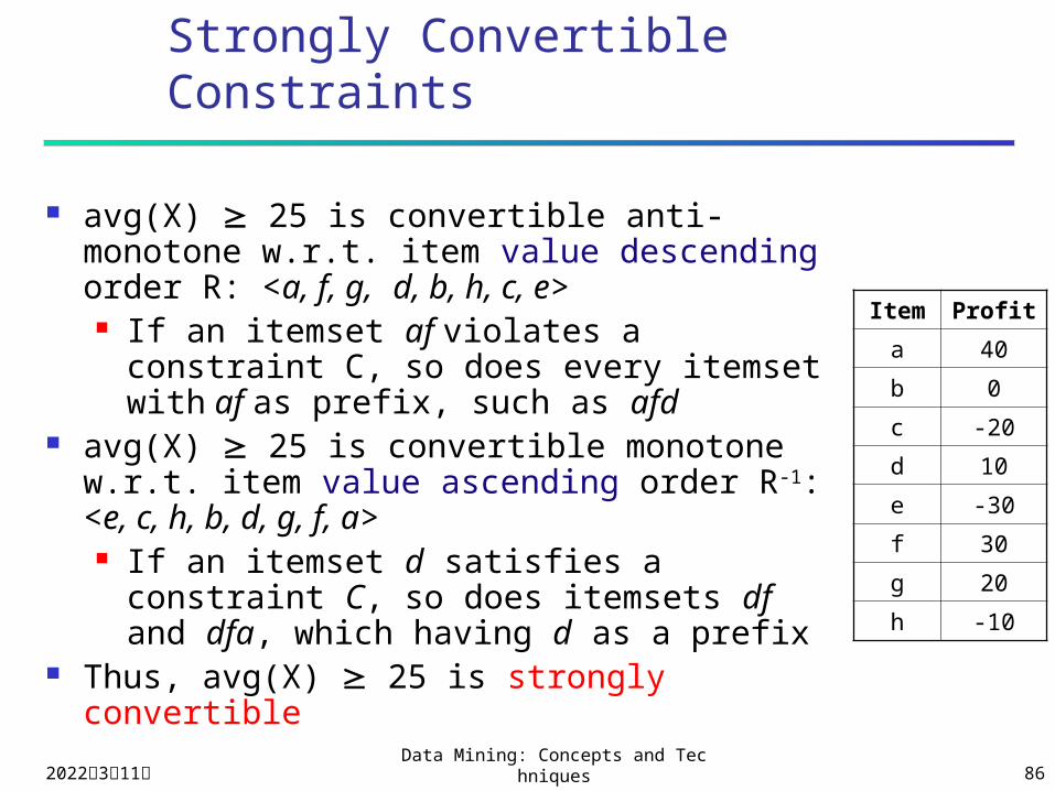
Strongly Convertible Constraints
avg(X) 25 is convertible anti-monotone w.r.t. item value descending order R: <a, f, g, d, b, h, c, e> If an itemset af violates a constraint C,
so does every itemset with af as prefix, such as afd
avg(X) 25 is convertible monotone w.r.t. item value ascending order R-1: <e, c, h, b, d, g, f, a> If an itemset d satisfies a constraint C,
so does itemsets df and dfa, which having d as a prefix
Thus, avg(X) 25 is strongly convertible
Item Profit
a 40
b 0
c -20
d 10
e -30
f 30
g 20
h -10
2023年4月19日Data Mining: Concepts and Technique
s 87
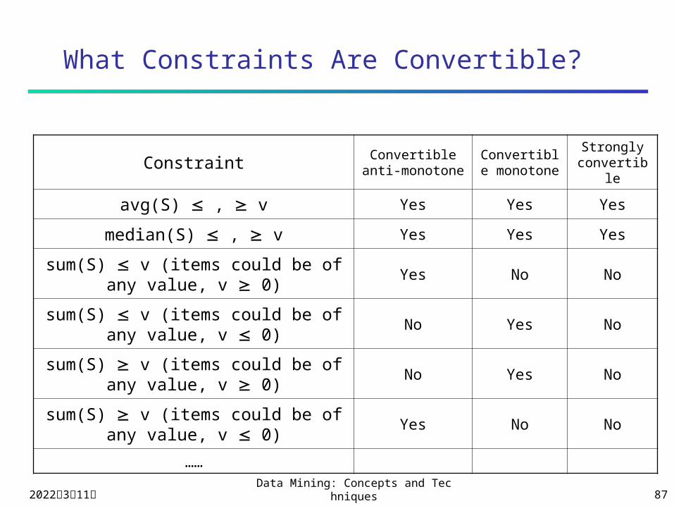
What Constraints Are Convertible?
Constraint Convertible anti-monotone
Convertible monotone
Strongly convertible
avg(S) , v Yes Yes Yes
median(S) , v Yes Yes Yes
sum(S) v (items could be of any value, v 0)
Yes No No
sum(S) v (items could be of any value, v 0)
No Yes No
sum(S) v (items could be of any value, v 0)
No Yes No
sum(S) v (items could be of any value, v 0)
Yes No No
……
2023年4月19日Data Mining: Concepts and Technique
s 88
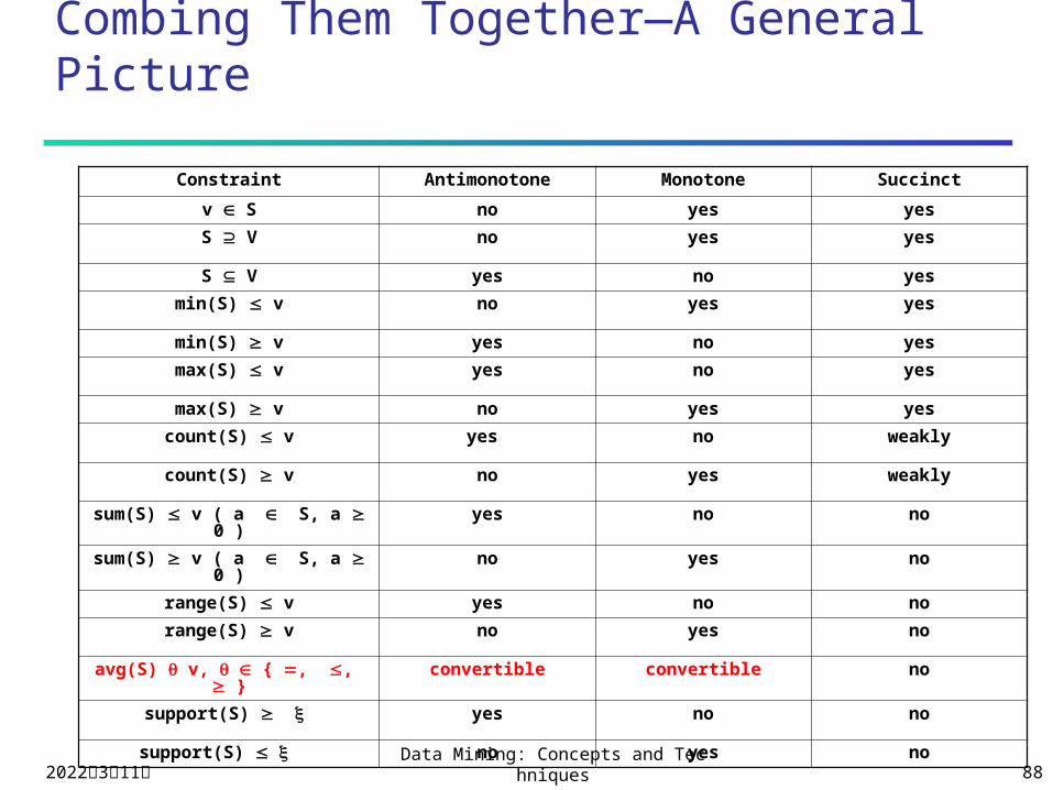
Combing Them Together—A General Picture
Constraint Antimonotone Monotone Succinct
v S no yes yes
S V no yes yes
S V yes no yes
min(S) v no yes yes
min(S) v yes no yes
max(S) v yes no yes
max(S) v no yes yes
count(S) v yes no weakly
count(S) v no yes weakly
sum(S) v ( a S, a 0 ) yes no no
sum(S) v ( a S, a 0 ) no yes no
range(S) v yes no no
range(S) v no yes no
avg(S) v, { , , } convertible convertible no
support(S) yes no no
support(S) no yes no
2023年4月19日Data Mining: Concepts and Technique
s 89
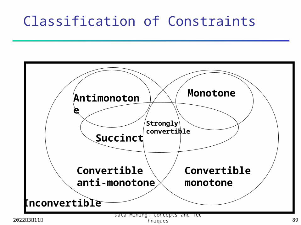
Classification of Constraints
Convertibleanti-monotone
Convertiblemonotone
Stronglyconvertible
Inconvertible
Succinct
Antimonotone
Monotone
2023年4月19日Data Mining: Concepts and Technique
s 90
Chapter 5 (in fact 8.3): Mining Association Rules in Large Databases
Association rule mining
Algorithms Apriori and FP-Growth
Max and closed patterns
Mining various kinds of association/correlation
rules
Constraint-based association mining
Sequential pattern mining
2023年4月19日Data Mining: Concepts and Technique
s 91
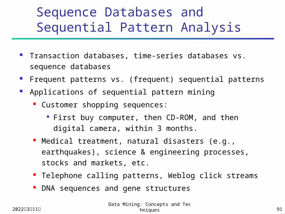
Sequence Databases and Sequential Pattern Analysis
Transaction databases, time-series databases vs. sequence databases
Frequent patterns vs. (frequent) sequential patterns Applications of sequential pattern mining
Customer shopping sequences: First buy computer, then CD-ROM, and then digital
camera, within 3 months. Medical treatment, natural disasters (e.g.,
earthquakes), science & engineering processes, stocks and markets, etc.
Telephone calling patterns, Weblog click streams DNA sequences and gene structures
2023年4月19日Data Mining: Concepts and Technique
s 92
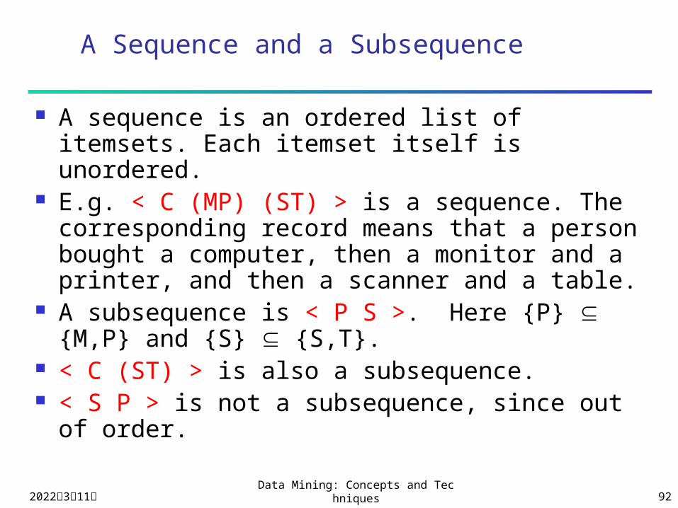
A Sequence and a Subsequence
A sequence is an ordered list of itemsets. Each itemset itself is unordered.
E.g. < C (MP) (ST) > is a sequence. The corresponding record means that a person bought a computer, then a monitor and a printer, and then a scanner and a table.
A subsequence is < P S >. Here {P} {M,P} and {S} {S,T}.
< C (ST) > is also a subsequence. < S P > is not a subsequence, since out of
order.
2023年4月19日Data Mining: Concepts and Technique
s 93
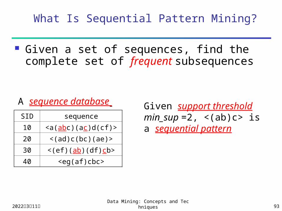
What Is Sequential Pattern Mining?
Given a set of sequences, find the complete set of frequent subsequences
A sequence database Given support threshold min_sup =2, <(ab)c> is a sequential pattern
SID sequence
10 <a(abc)(ac)d(cf)>
20 <(ad)c(bc)(ae)>
30 <(ef)(ab)(df)cb>
40 <eg(af)cbc>
2023年4月19日Data Mining: Concepts and Technique
s 94
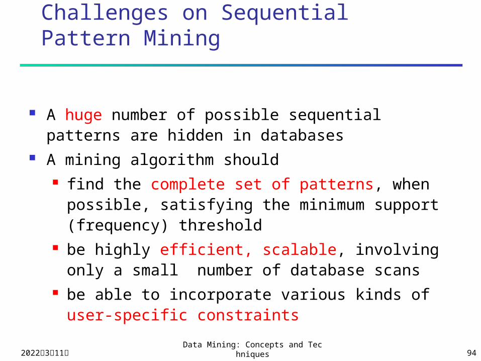
Challenges on Sequential Pattern Mining
A huge number of possible sequential patterns are hidden in databases
A mining algorithm should find the complete set of patterns, when
possible, satisfying the minimum support (frequency) threshold
be highly efficient, scalable, involving only a small number of database scans
be able to incorporate various kinds of user-specific constraints
2023年4月19日Data Mining: Concepts and Technique
s 95
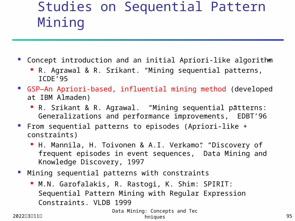
Studies on Sequential Pattern Mining
Concept introduction and an initial Apriori-like algorithm R. Agrawal & R. Srikant. “Mining sequential patterns,” ICDE’95
GSP—An Apriori-based, influential mining method (developed at IBM Almaden)
R. Srikant & R. Agrawal. “Mining sequential patterns: Generalizations and performance improvements,” EDBT’96
From sequential patterns to episodes (Apriori-like + constraints) H. Mannila, H. Toivonen & A.I. Verkamo. “Discovery of
frequent episodes in event sequences,” Data Mining and Knowledge Discovery, 1997
Mining sequential patterns with constraints M.N. Garofalakis, R. Rastogi, K. Shim: SPIRIT: Sequential
Pattern Mining with Regular Expression Constraints. VLDB 1999

2023年4月19日Data Mining: Concepts and Technique
s 96
A Basic Property of Sequential Patterns: Apriori
A basic property: Apriori (Agrawal & Sirkant’94) If a sequence S is not frequent Then none of the super-sequences of S is frequent E.g, <hb> is infrequent so do <hab> and <(ah)b>
<a(bd)bcb(ade)>50
<(be)(ce)d>40
<(ah)(bf)abf>30
<(bf)(ce)b(fg)>20
<(bd)cb(ac)>10
SequenceSeq. ID Given support threshold min_sup =2
2023年4月19日Data Mining: Concepts and Technique
s 97
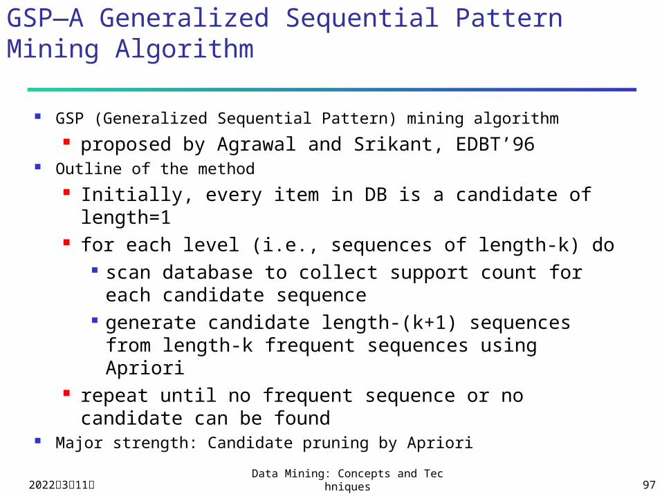
GSP—A Generalized Sequential Pattern Mining Algorithm
GSP (Generalized Sequential Pattern) mining algorithm proposed by Agrawal and Srikant, EDBT’96
Outline of the method Initially, every item in DB is a candidate of
length=1 for each level (i.e., sequences of length-k) do
scan database to collect support count for each candidate sequence
generate candidate length-(k+1) sequences from length-k frequent sequences using Apriori
repeat until no frequent sequence or no candidate can be found
Major strength: Candidate pruning by Apriori
2023年4月19日Data Mining: Concepts and Technique
s 98
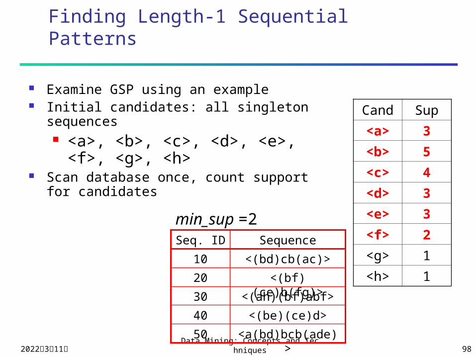
Finding Length-1 Sequential Patterns
Examine GSP using an example Initial candidates: all singleton sequences
<a>, <b>, <c>, <d>, <e>, <f>, <g>, <h>
Scan database once, count support for candidates
<a(bd)bcb(ade)>50
<(be)(ce)d>40
<(ah)(bf)abf>30
<(bf)(ce)b(fg)>20
<(bd)cb(ac)>10
SequenceSeq. ID
min_sup =2
Cand Sup
<a> 3
<b> 5
<c> 4
<d> 3
<e> 3
<f> 2
<g> 1
<h> 1
2023年4月19日Data Mining: Concepts and Technique
s 99
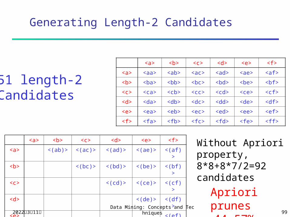
Generating Length-2 Candidates
<a> <b> <c> <d> <e> <f>
<a> <aa> <ab> <ac> <ad> <ae> <af>
<b> <ba> <bb> <bc> <bd> <be> <bf>
<c> <ca> <cb> <cc> <cd> <ce> <cf>
<d> <da> <db> <dc> <dd> <de> <df>
<e> <ea> <eb> <ec> <ed> <ee> <ef>
<f> <fa> <fb> <fc> <fd> <fe> <ff>
<a> <b> <c> <d> <e> <f>
<a> <(ab)> <(ac)> <(ad)> <(ae)> <(af)>
<b> <(bc)> <(bd)> <(be)> <(bf)>
<c> <(cd)> <(ce)> <(cf)>
<d> <(de)> <(df)>
<e> <(ef)>
<f>
51 length-2Candidates
Without Apriori property,8*8+8*7/2=92 candidates
Apriori prunes 44.57% candidates
2023年4月19日Data Mining: Concepts and Technique
s 101
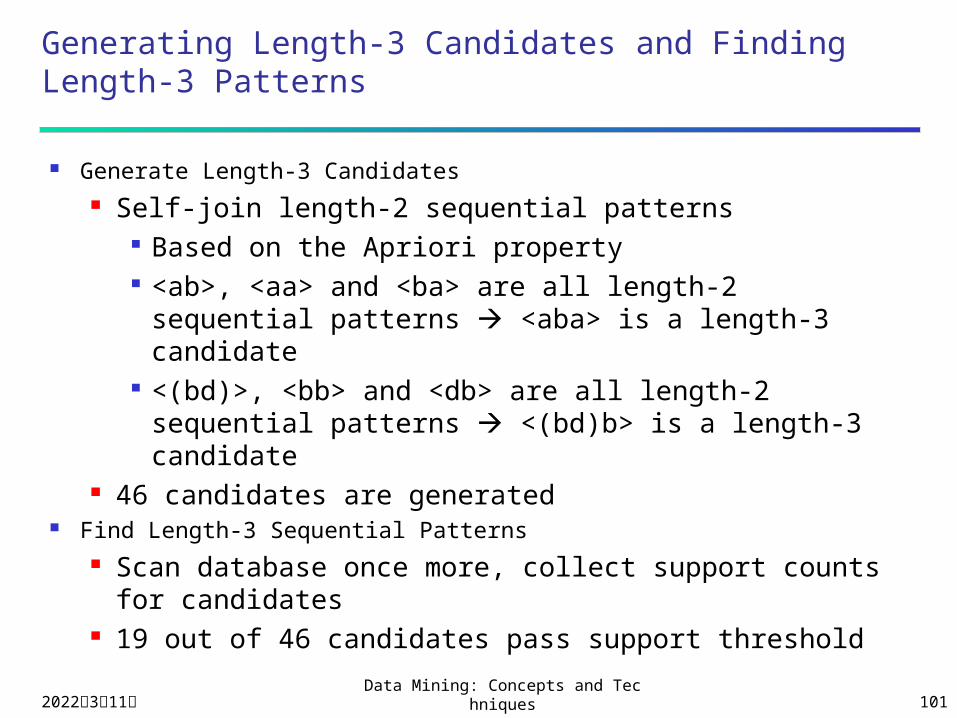
Generating Length-3 Candidates and Finding Length-3 Patterns
Generate Length-3 Candidates Self-join length-2 sequential patterns
Based on the Apriori property <ab>, <aa> and <ba> are all length-2 sequential
patterns <aba> is a length-3 candidate <(bd)>, <bb> and <db> are all length-2
sequential patterns <(bd)b> is a length-3 candidate
46 candidates are generated Find Length-3 Sequential Patterns
Scan database once more, collect support counts for candidates
19 out of 46 candidates pass support threshold
2023年4月19日Data Mining: Concepts and Technique
s 102
The GSP Mining Process
<a> <b> <c> <d> <e> <f> <g> <h>
<aa> <ab> … <af> <ba> <bb> … <ff> <(ab)> … <(ef)>
<abb> <aab> <aba> <baa> <bab> …
<abba> <(bd)bc> …
<(bd)cba>
1st scan: 8 cand. 6 length-1 seq. pat.
2nd scan: 51 cand. 19 length-2 seq. pat. 10 cand. not in DB at all
3rd scan: 46 cand. 19 length-3 seq. pat. 20 cand. not in DB at all
4th scan: 8 cand. 6 length-4 seq. pat.
5th scan: 1 cand. 1 length-5 seq. pat.
Cand. cannot pass sup. threshold
Cand. not in DB at all
<a(bd)bcb(ade)>50
<(be)(ce)d>40
<(ah)(bf)abf>30
<(bf)(ce)b(fg)>20
<(bd)cb(ac)>10
SequenceSeq. ID
min_sup =2
2023年4月19日Data Mining: Concepts and Technique
s 104
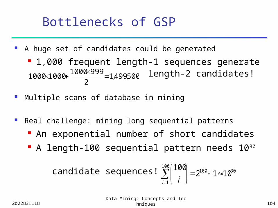
Bottlenecks of GSP
A huge set of candidates could be generated
1,000 frequent length-1 sequences generate length-2
candidates!
Multiple scans of database in mining
Real challenge: mining long sequential patterns
An exponential number of short candidates A length-100 sequential pattern needs 1030
candidate sequences!
500,499,12
999100010001000
30100100
1
1012100
i i
2023年4月19日Data Mining: Concepts and Technique
s 105
PrefixSpan: Prefix-Projected Sequential Pattern Mining
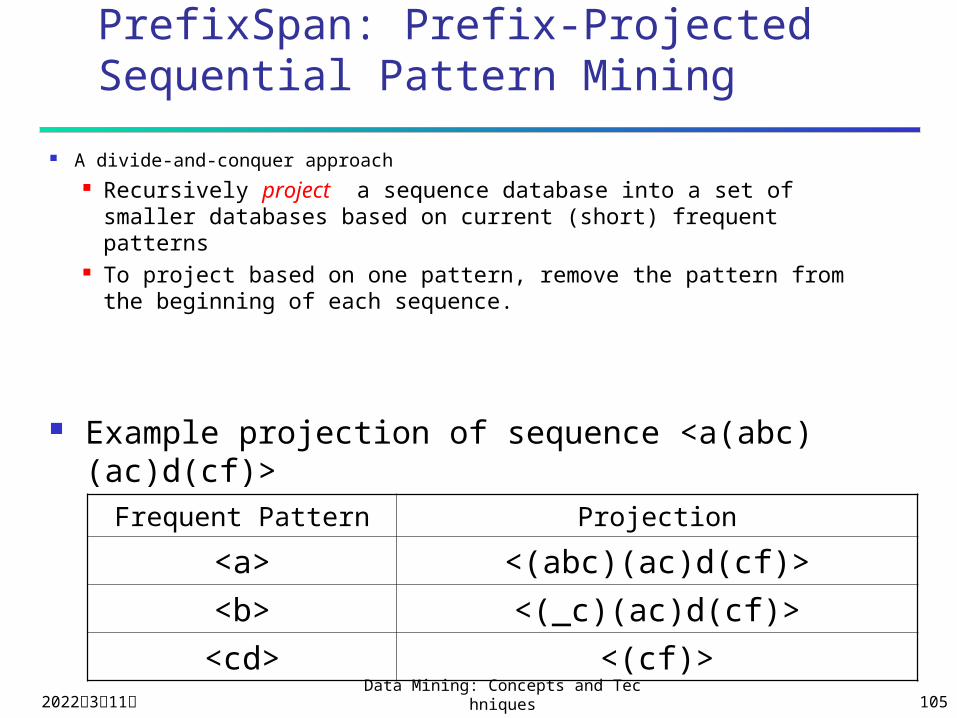
A divide-and-conquer approach Recursively project a sequence database into a set of
smaller databases based on current (short) frequent patterns To project based on one pattern, remove the pattern from
the beginning of each sequence.
Example projection of sequence <a(abc)(ac)d(cf)>
Frequent Pattern Projection
<a> <(abc)(ac)d(cf)>
<b> <(_c)(ac)d(cf)>
<cd> <(cf)>

2023年4月19日Data Mining: Concepts and Technique
s 106
Mining Sequential Patterns by Prefix Projections
Step 1: find length-1 sequential patterns <a>, <b>, <c>, <d>, <e>, <f>
Step 2: divide search space. The complete set of seq. pat. can be partitioned into 6 subsets: The ones having prefix <a>; The ones having prefix <b>; … The ones having prefix <f>
SID sequence
10 <a(abc)(ac)d(cf)>
20 <(ad)c(bc)(ae)>
30 <(ef)(ab)(df)cb>
40 <eg(af)cbc>
2023年4月19日Data Mining: Concepts and Technique
s 107
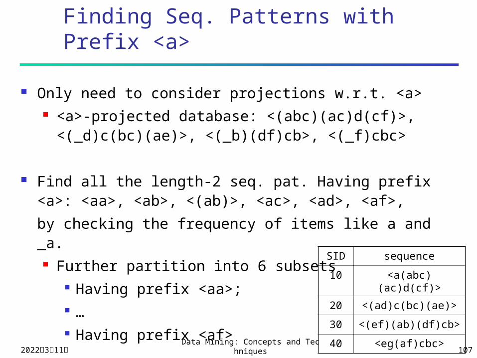
Finding Seq. Patterns with Prefix <a>
Only need to consider projections w.r.t. <a> <a>-projected database: <(abc)(ac)d(cf)>,
<(_d)c(bc)(ae)>, <(_b)(df)cb>, <(_f)cbc>
Find all the length-2 seq. pat. Having prefix <a>: <aa>, <ab>, <(ab)>, <ac>, <ad>, <af>,
by checking the frequency of items like a and _a. Further partition into 6 subsets
Having prefix <aa>; … Having prefix <af>
SID sequence
10 <a(abc)(ac)d(cf)>
20 <(ad)c(bc)(ae)>
30 <(ef)(ab)(df)cb>
40 <eg(af)cbc>
2023年4月19日Data Mining: Concepts and Technique
s 108
Completeness of PrefixSpan
SID sequence
10 <a(abc)(ac)d(cf)>
20 <(ad)c(bc)(ae)>
30 <(ef)(ab)(df)cb>
40 <eg(af)cbc>
SDB
Length-1 sequential patterns<a>, <b>, <c>, <d>, <e>, <f>
<a>-projected database<(abc)(ac)d(cf)><(_d)c(bc)(ae)><(_b)(df)cb><(_f)cbc>
Length-2 sequentialpatterns<aa>, <ab>, <(ab)>,<ac>, <ad>, <af>
Having prefix <a>
Having prefix <aa>
<aa>-proj. db … <af>-proj. db
Having prefix <af>
<b>-projected database …
Having prefix <b>Having prefix <c>, …, <f>
… …
2023年4月19日Data Mining: Concepts and Technique
s 109
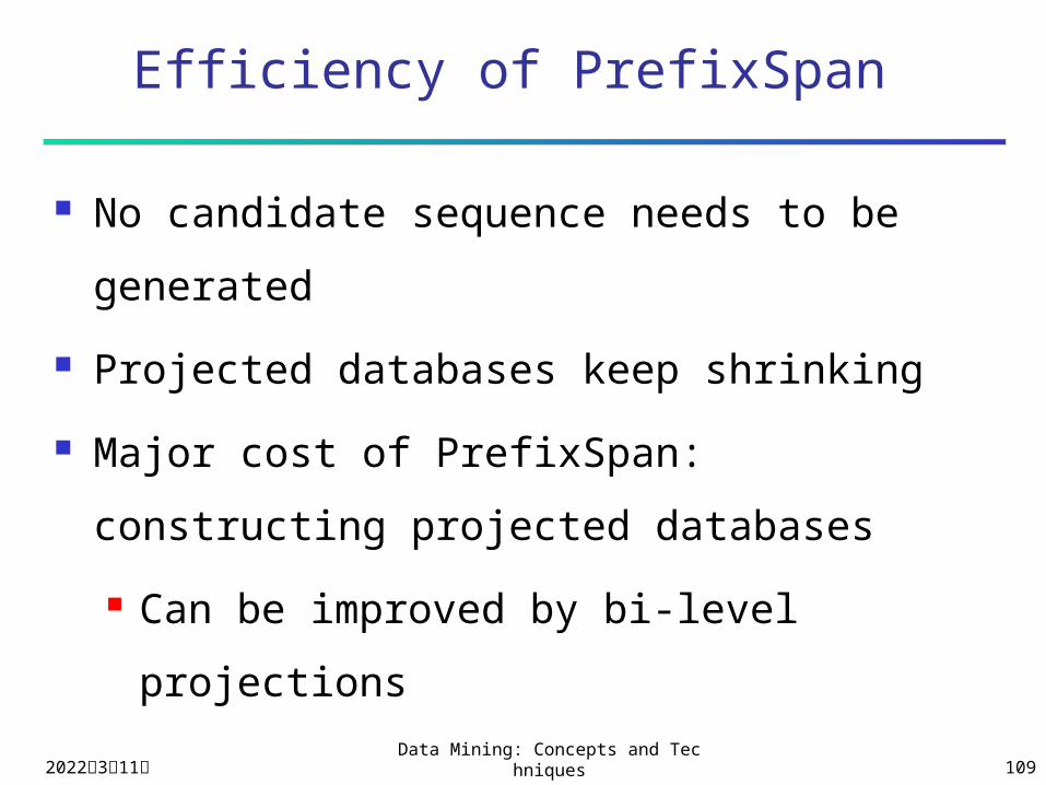
Efficiency of PrefixSpan
No candidate sequence needs to be
generated
Projected databases keep shrinking
Major cost of PrefixSpan: constructing
projected databases
Can be improved by bi-level projections
2023年4月19日Data Mining: Concepts and Technique
s 110
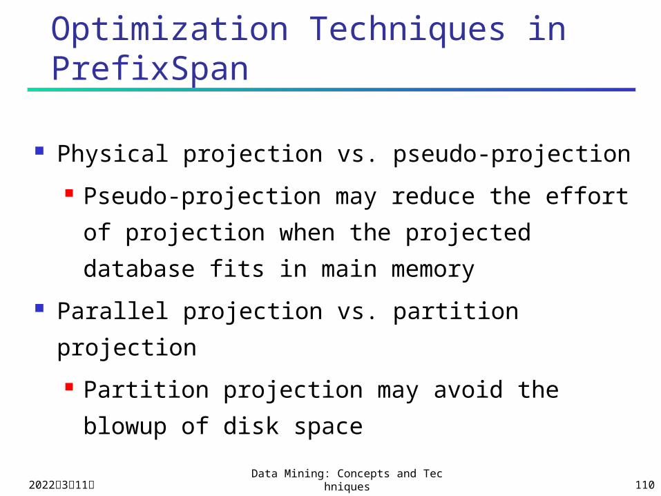
Optimization Techniques in PrefixSpan
Physical projection vs. pseudo-projection
Pseudo-projection may reduce the effort
of projection when the projected database
fits in main memory
Parallel projection vs. partition projection
Partition projection may avoid the blowup
of disk space
2023年4月19日Data Mining: Concepts and Technique
s 111
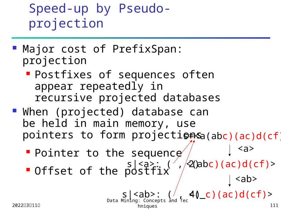
Speed-up by Pseudo-projection
Major cost of PrefixSpan: projection Postfixes of sequences often
appear repeatedly in recursive projected databases
When (projected) database can be held in main memory, use pointers to form projections Pointer to the sequence Offset of the postfix
s=<a(abc)(ac)d(cf)>
<(abc)(ac)d(cf)>
<(_c)(ac)d(cf)>
<a>
<ab>
s|<a>: ( , 2)
s|<ab>: ( , 4)
2023年4月19日Data Mining: Concepts and Technique
s 112
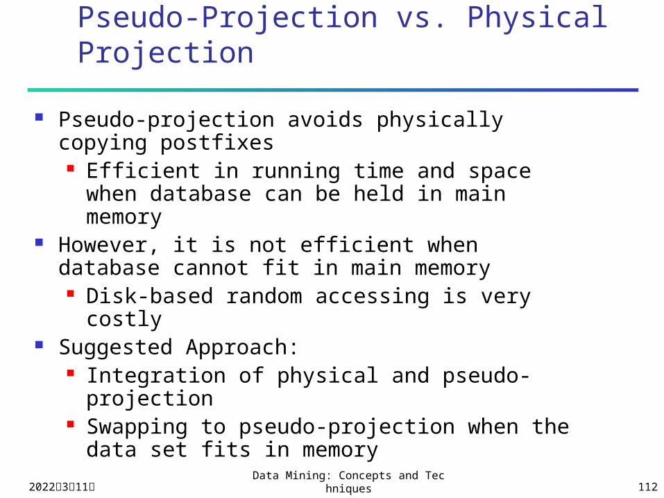
Pseudo-Projection vs. Physical Projection
Pseudo-projection avoids physically copying postfixes Efficient in running time and space when
database can be held in main memory However, it is not efficient when database
cannot fit in main memory Disk-based random accessing is very costly
Suggested Approach: Integration of physical and pseudo-
projection Swapping to pseudo-projection when the
data set fits in memory
2023年4月19日Data Mining: Concepts and Technique
s 113
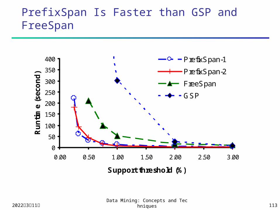
PrefixSpan Is Faster than GSP and FreeSpan
0
50
100
150
200
250
300
350
400
0.00 0.50 1.00 1.50 2.00 2.50 3.00
Support threshold (%)
Ru
nti
me
(sec
on
d)
PrefixSpan-1
PrefixSpan-2
FreeSpan
GSP
2023年4月19日Data Mining: Concepts and Technique
s 114
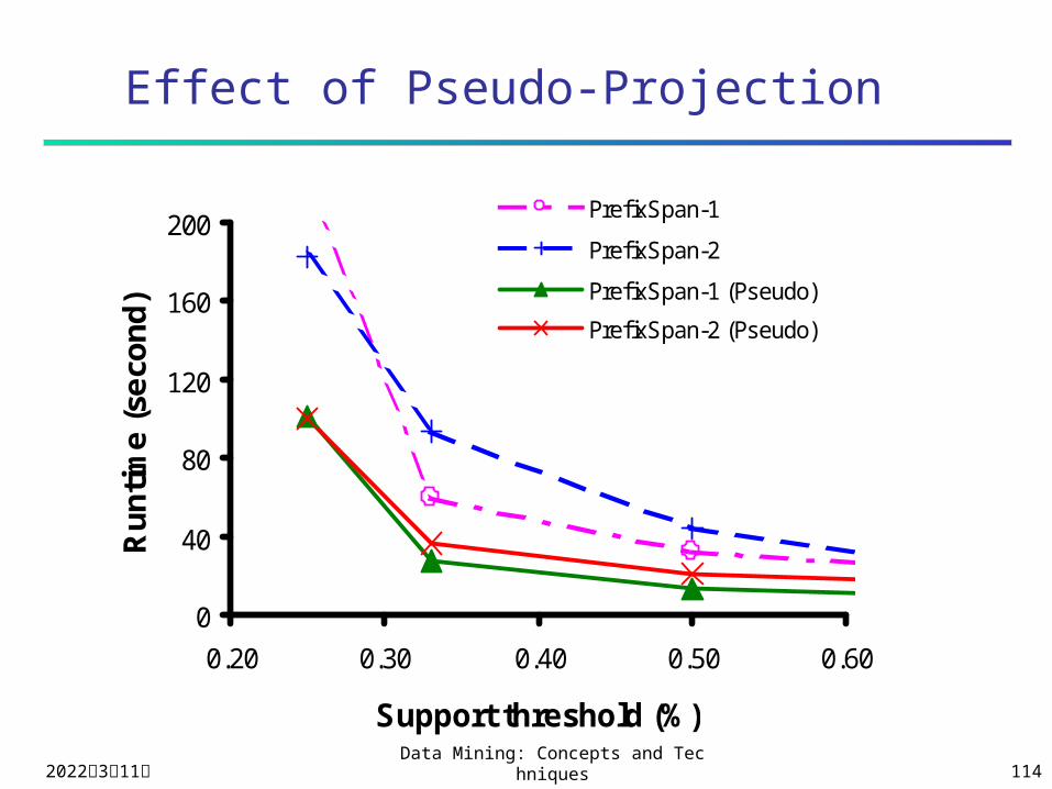
Effect of Pseudo-Projection
0
40
80
120
160
200
0.20 0.30 0.40 0.50 0.60
Support threshold (%)
Ru
nti
me
(se
con
d)
PrefixSpan-1
PrefixSpan-2
PrefixSpan-1 (Pseudo)
PrefixSpan-2 (Pseudo)
2023年4月19日Data Mining: Concepts and Technique
s 115
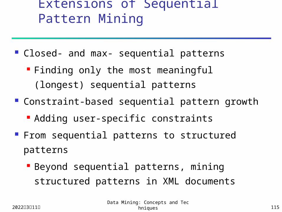
Extensions of Sequential Pattern Mining
Closed- and max- sequential patterns
Finding only the most meaningful (longest)
sequential patterns
Constraint-based sequential pattern growth
Adding user-specific constraints
From sequential patterns to structured
patterns
Beyond sequential patterns, mining
structured patterns in XML documents
2023年4月19日Data Mining: Concepts and Technique
s 116
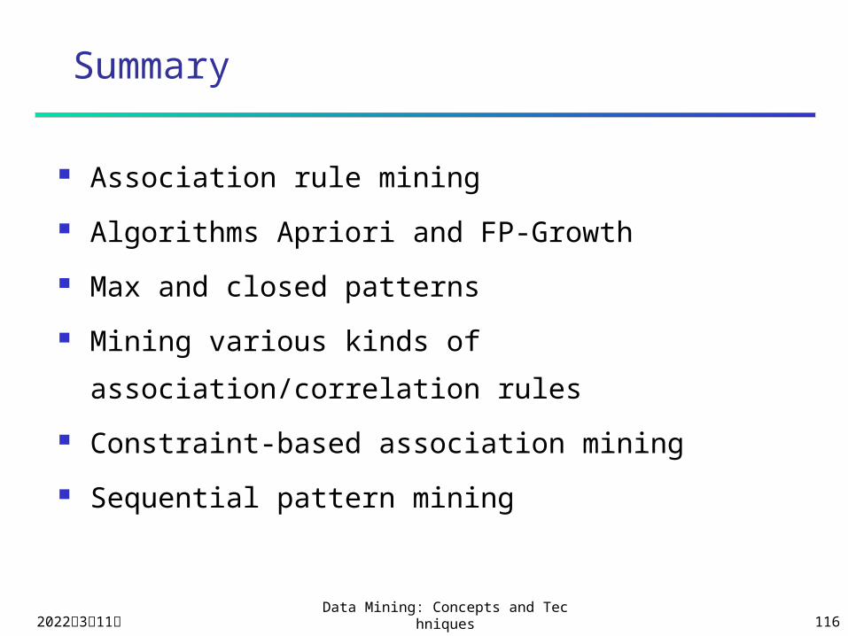
Summary
Association rule mining
Algorithms Apriori and FP-Growth
Max and closed patterns
Mining various kinds of association/correlation
rules
Constraint-based association mining
Sequential pattern mining