2015 Valuation Basic Table Report

Joint Academy of Actuaries’ Life Experience Committee and Society of Actuaries’ Preferred Mortality Oversight Group

Valuation Basic Table Team

March 2018 (revised September 2018)

The American Academy of Actuaries is a 19,000-member professional association whose mission is to serve the public and the U.S. actuarial profession. For more than 50 years, the Academy has assisted public policymakers on all levels by providing leadership, objective expertise, and actuarial advice on risk and financial security issues. The Academy also sets qualification, practice, and professionalism standards for actuaries in the United States.

The Society of Actuaries (SOA) is an educational, research and professional organization dedicated to serving the public, its members and its candidates. The SOA's mission is to advance actuarial knowledge and to enhance the ability of actuaries to provide expert advice and relevant solutions for financial, business and societal problems. The SOA's vision is for actuaries to be the leading professionals in the measurement and management of risk.

2

2015 Valuation Basic Table Report

Caveat and Disclaimer This study is published by the Society of Actuaries (SOA) and contains information from a variety of sources. It may or may not reflect the experience of any individual company. The study is for informational purposes only and should not be construed as professional or financial advice. The SOA does not recommend or endorse any particular use of the information provided in this study. The SOA makes no warranty, express or implied, or representation whatsoever and assumes no liability in connection with the use or misuse of this study. Copyright ©2018 All rights reserved by the Society of Actuaries Copyright ©2018 All rights reserved by the American Academy of Actuaries

AUTHOR

Academy/SOA Valuation Basic Table Team

3

TABLE OF CONTENTS

Preface: Revisions Made to this Report Subsequent to March 2018 ........................................ 4

Members of the Valuation Basic Table Team .......................................................................... 5

I. Purpose of the Study ........................................................................................................... 6

II. Background and Scope ....................................................................................................... 7

III. General Comments on the Table Development Process ...................................................... 8

IV. Underlying Data .............................................................................................................. 13

V. Development of 2015 VBT Primary Table .......................................................................... 19

VI. Development of 2015 Relative Risk (RR) Tables ................................................................ 51

VII. Composite Primary Mortality Tables ............................................................................... 58

VIII. Comparison to 2008 VBT Tables .................................................................................... 60

IX. MIB Analysis and Validation ............................................................................................ 65

Appendix A. SOA ILEC Underlying Experience Data 2002-09 .................................................. 66

Appendix B. Adjustments of Experience to Current Business Distribution .............................. 68

Appendix C. Development of Age Last Birthday (ALB) Tables ................................................. 69

Appendix D. Sample RR Mortality Rate Calculations .............................................................. 71

Appendix E. Monotonicity Adjustments ................................................................................ 72

Appendix F. Preferred Wear-off Factors ................................................................................ 73

Appendix G. Preferred Wear-off Factors ............................................................................... 77

Appendix H. 2004-2009 Individual Life Data .......................................................................... 87

Appendix I. Preferred vs. Aggregate Exposure ....................................................................... 89

Appendix J. Underwriting Class Adjustments ........................................................................ 90

Appendix K. Calculation of Age-Last-Birthday (ALB) Rates ..................................................... 91

Appendix L. Mortality Improvement Factors ......................................................................... 93

About The Society of Actuaries ............................................................................................. 94

4

Preface: Revisions Made to this Report Subsequent to March 2018

September 2018 Updates • Section 5.J. was updated with a reference to Appendix L. • Appendix L – Mortality Improvement Factors was added.

5

Members of the Valuation Basic Table Team

Mary Bahna-Nolan, FSA, MAAA, CERA, Chair

SOA Staff:

Jack Luff, FSA, FCIA, MAAA

Mervyn Kopinsky, FSA, EA

Cynthia MacDonald, FSA, MAAA

Patrick Nolan, FSA, MAAA

Korrel Rosenberg

Muz Waheed, FSA, MAAA, CERA

Special thanks to the following individuals and businesses which made significant contributions to the development of the VBT Tables:

Steven Craighead, ASA, MAAA, CERA

Phillip Adams, FSA, MAAA, CERA

John Fenton, FSA, MAAA

Milliman USA

Willis Towers Watson

Mike Bertsche, FSA, MAAA Vera Ljucovic, FSA, FCIA

Jay Biehl, FSA, MAAA Frank McCarthy, FSA

Suzanne Chapa, FSA, MAAA Marianne Purushotham, FSA, MAAA

Sanjeev Chaudhuri, FSA, MAAA Chuck Ritzke, FSA, MAAA

Lilian Cheung, FSA, MAAA Nick Sales, FSA, MAAA

Tom Edwalds, FSA, ACAS, MAAA Bruce Schobel, FSA, MAAA

Henry Egesi, FSA, MAAA Tomasz Serbinowski, PhD, FSA

Dieter Gaubatz, FSA, FCIA, MAAA Kim Steiner, FSA, MAAA

Ed Hui, FSA, CFA, MAAA Andy Ware, FSA, MAAA

Al Klein, FSA, MAAA

6

I. Purpose of the Study

The primary purposes of the study are:

1. To develop industry experience mortality tables that reflect fully underwritten ordinary life business including standard and preferred mortality risks. These tables are to be considered the “industry tables” within the new NAIC principles based reporting standards for valuing life insurance, specifically under the Valuation Manual, Section 20 (VM-20).

VM-20 applies to new issues on or after the operative date of the Valuation Manual. Therefore, the industry tables are to reflect historical experience while also taking into consideration changes that were driving historical experience that are not expected on a new issue go forward basis. For example, an adjustment was made to the data to recognize differences in experience from different underwriting eras and smooth out the volatility due to anti-select mortality in the years following the shocks to the underwriting programs and subsequent replacement activity.

2. To develop a table or tables to be used as the basis for applying loading in order to develop a new Commissioners’ Standard Only mortality table (CSO) for use in determining net premium reserves under CRVM and for adherence to standard nonforfeiture and tax regulations.

7

II. Background and Scope

The Valuation Basic Table Team (Team), as requested by the NAIC’s Life Actuarial Task Force (LATF), was to produce a set of valuation basic mortality tables (before inclusion of margins necessary to make the table suitable for standard valuation purposes) for individual life insurance products that reflect standard and preferred underwriting criteria. These tables were to become the industry tables for use in determining a company’s Prudent Estimate Mortality Assumption within chapter VM-20 of the Valuation Manual for Principles Based Reserves (PBR). The scope did not include analysis of the mortality experience or development of mortality tables for guaranteed issue, simplified issue, or pre-need coverage. This section of the report documents the data, assumptions, and process the Team used to develop the 2015 Valuation Basic Table (2015 VBT).

The 2015 VBT consists of the Primary Table (Male, Female, Smoker, Nonsmoker, and Composite), 10 Relative Risk (RR) tables for nonsmokers (male and female), and 4 RR tables for smokers (male and female). The RR tables reflect the range of expected mortality from super-preferred to residual standard risk. Rates for juvenile ages are included in the composite tables. The tables are on a select and ultimate and ultimate-only basis, and are available on an age nearest and an age last birthday basis. Unlike the 2008 VBT, there is no Limited Underwriting Table associated with the 2015 VBT.

The main source of underlying data (2002-2009 data) used in developing the 2015 VBT was compiled from four separate Society of Actuaries (SOA) Individual Life Experience Committee's (ILEC) intercompany studies1 (2002-2009 studies) attached in Appendix A of this report. These studies included $30.7 trillion in exposure by amount; 266 million in exposure by number of policies; and nearly 2.6 million death claims from 51 contributing companies, including over 577,000 deaths in the select period, as defined in Section V.H of this document, and over 1,982,000 deaths in the ultimate period. Not all companies contributed data in each study period. No data was excluded in the study period. Since testing for smoking or tobacco usage did not become common until the early 1980s, a significant portion of the underlying select period data is smoker and nonsmoker distinct, whereas the ultimate period data was nearly all issued on a composite basis. Therefore, the Team determined smoker prevalence rates for the ultimate data via extrapolation of the smoker-distinct select rates at late durations within the select period. See Section IV.D for further discussion.

1 The 2002-2004 Individual Life Experience Report, the 2004-2005 Individual Life Experience Report, the 2005-2007 Individual Life Experience Report, and the 2007-2009 Individual Life Experience Report. The compiled 2002-2009 data will be made available with the next ILEC study, expected to be released in summer 2017.

8

III. General Comments on the Table Development Process

To develop the 2015 VBT tables, there were multiple considerations. To address these, the Team was broken into the following eight subgroups:

1. Older age mortality: focused on special considerations regarding the older age mortality, specifically the slope of the mortality at the oldest ages and the ultimate omega mortality rate.

• Chair: Ed Hui

• Members: Mike Bertsche

Lilian Cheung

John Fenton*

Dieter Gaubatz

Al Klein

Vera Ljucovic

Nick Sales

Bruce Schobel

2. Juvenile mortality: focused on special considerations regarding juvenile mortality (ages 0 to 17).

• Chair: Chuck Ritzke

• Members: Tom Edwalds

Henry Egesi

3. Select period & Preferred Wear-off: focused on determination of the select period from both the underlying data and considerations where historical experience may no longer be applicable for new issues and specific underwriting performed today. This subgroup also researched and studied the underlying experience for patterns of preferred mortality wear-off.

• Chair: Jay Biehl

• Members: Michael Bertsche

Suzanne Chapa

Sanjeev Chaudhuri

9

Tom Edwalds

Dieter Gaubatz

Ed Hui

Tomasz Serbinowski

4. Mortality improvement: this subgroup focused on both the generational improvement from the mid-point of the experience data exposure period as well as durational improvement to project the experience from the end of the experience period (2009) to mid-year 2015.

• Chair: Marianne Purushotham

• Members: Jay Biehl

Bruce Schobel

Sanjeev Chaudhuri

5. Graduation: this subgroup focused on determination of the graduation approach as well as graduating the ultimate and select period data and performed monotonicity validation.

• Chair: Tom Edwalds

• Members: Phillip Adams*

Steve Craighead*

Nick Sales

Tomasz Serbinowski

6. Modeling: this subgroup prepared models for analysis of the graduated mortality rates relative to the raw data and other mortality basis such as the 2008 VBT to understand the impacts of the changes in the new table.

• Chair: Tom Edwalds

• Members: Suzanne Chapa

Henry Egesi

Marianne Purushotham

Chuck Ritzke

* Not a member of the official VBT Team, but significant contributor to the work product.

10

7. Industry liaison: This team, consisting of Mary Bahna-Nolan and Andy Ware, interacted with industry trade groups such as the ACLI to make sure certain industry considerations were evaluated and taken into consideration as well as to solicit input, when necessary.

The Team began by developing ultimate mortality rates based on the underlying experience. To develop the ultimate mortality rates, the Team:

• Determined whether to exclude any experience from the 2002-2009 studies from the analysis;

• Reviewed external studies and research to determine the most applicable population mortality at the older ages;

• If and how to augment the mortality experience for juveniles;

• Determined how to augment the 2002-2009 studies experience data with the results of other mortality research;

• Determined the omega rate; and

• Determined the appropriate graduation methodology.

Once the ultimate mortality rates were developed, the Team developed the select and ultimate tables for male and female, nonsmoker and smoker risks (hereafter referred to as the Primary Tables) by determining the following items:

• The issue age limits;

• The select period;

• How to augment the mortality experience for juveniles;

• How to augment the mortality experience for smoker risks;

• Mortality improvement factors and any additional adjustments to the underlying experience; and

• The appropriate graduation methodology.

11

Once the Primary Tables were completed, the Team worked to split these tables into multiple tables that reflect a range of expected mortality from preferred underwriting programs, ranging from super-preferred to residual standard. To do so, the Team determined:

• The number of tables or representative risk classes;

• The relationship between the specific underwriting criteria and the mortality experience for that particular level of underwriting; and

• How quickly the preferred underwriting effects wear off (this is in addition to the wear-off of age and amount requirements from general underwriting).

The Team performed the mortality experience analysis and table development on an age nearest birthday basis. A conversion algorithm, consistent with that used in previous valuation basic table development, was then applied to develop the tables on an age last birthday basis. This algorithm is shown in Appendix C of this report.

Each subgroup analyzed the data specific to their respective focus areas and then presented back to the broader Team for final decision as to the structure of the 2015 VBT table. Throughout the process, the Team presented findings and solicited regulator and industry feedback via presentations at NAIC LATF meetings and LATF conference calls as well as various presentations at Academy and SOA meetings and webinars.

The table was initially developed as the 2014 VBT; however, due to delays in the development of the table, the Team solicited and received guidance from LATF to project the table one additional year to 2015. The improvement factors that were used for projecting the table from 2009 to 2014 were used to project the experience mortality one additional year.

The table was exposed by LATF to the insurance industry for comment and feedback twice – once for the Primary Tables and again for the Relative Risk Tables as well as updates to the Primary Tables based on the initial round of comments and feedback. There were minimal comments submitted for each of the exposures, and the comments were incorporated into the final 2015 VBT tables.

12

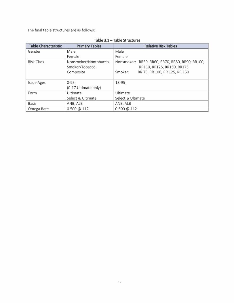
The final table structures are as follows:

Table 3.1 – Table Structures Table Characteristic Primary Tables Relative Risk Tables

Gender Male Female

Male Female

Risk Class Nonsmoker/Nontobacco Smoker/Tobacco Composite

Nonsmoker: RR50, RR60, RR70, RR80, RR90, RR100, RR110, RR125, RR150, RR175

Smoker: RR 75, RR 100, RR 125, RR 150

Issue Ages 0-95 (0-17 Ultimate only)

18-95

Form Ultimate Select & Ultimate

Ultimate Select & Ultimate

Basis ANB, ALB ANB, ALB Omega Rate 0.500 @ 112 0.500 @ 112

13

IV. Underlying Data

The 2015 VBT primary tables are based on the ILEC 2002-2009 industry experience, which has a large volume of data and exhibited a significant increase in exposure and number of claims over the studies underlying both the 2008 and 2001 VBT table development. The ILEC 02-09 data was obtained from 51 companies; of these, 21 were common to the 2008 VBT study and contributed data for each of the exposure years (“common companies”). As shown in the table below, the exposure by amount increased 345% over the exposure underlying the 2008 study and the number of claims increased by 271%.

Table 4.1 – Comparison of exposure, number of death claims and participating companies by recent studies supporting underlying VBT tables

Study/Table

Exposure Actual Deaths Companies

By Amount By Number Number Claims Number

2002-2009 / 2015 VBT $30.7 trillion 266 million 2.6 million 51

2002-2004/ 2008 VBT $6.9 trillion 75 million 0.7 million 35

1990-1995 / 2001 VBT $5.7 trillion 175 million ~ 1.25 million 21

Increase from 2008 VBT 345% 255% 271% 46%

Increase from 2001 VBT 439% 52% 100% 143%

One of the biggest concerns with the data used for the development of the 2015 VBT was the relatively large amount of more recent issue years not submitted on a preferred underwriting basis. Specifically, the number of policy years exposed in the first 10 durations in the preferred (including residual) data is 50,551,000. The corresponding number from all data is 96,617,000. This implies about a third of the data was not submitted on a preferred life basis. Upon request of the Team, SOA staff investigated the reason on a company specific basis.

After significant investigation, over six million exposure policy years were determined to be more accurately submitted on a preferred basis as opposed to their actual submission on an aggregate basis. This moves the relative percentage of preferred lives exposed from 52% of the submissions to 59%. It was not practical for the Team to ask the submitting companies to resubmit their data on the correct underwriting class basis; however, the Team did want to recognize and quantify the limitations in the data as submitted and more importantly to identify areas to investigate for initial data quality in future studies.

Table 4.2 – Adjustment to reclassify submitted data from aggregate to preferred risk basis Category Preferred Aggregate Total % Pref

Original Submission 50,551,000 46,066,000 96,617,000 52% Reclassified 6,160,000 (6,160,000) - Total 56,711,000 39,906,000 96,617,000 59%

Throughout this report, the expected basis used for analysis is the 2008 Valuation Basic Table RR 100 Table (2008 VBT RR 100) from the Final Report of the SOA’s Preferred Valuation Basic Table Team. For business issued on a smoker distinct basis, the expected basis is the 2008 VBT Sex Distinct, Smoker Distinct Tables;

14

for business issued on a composite basis, which includes much of the ultimate period data, the expected basis is the 2008 VBT Sex Distinct Composite Tables.

The overall level of mortality decreased significantly from that in the 2008 VBT table.

Table 4.3 – Comparison of A/E ratio by study period (E = 2008 VBT)

Study Period Male Female Aggregate Exposures (Trillion)

# Death Claims

2002-2004 (underlying 2008 VBT) 101.1% 100.5% 100.9% $7.4 699,890 2002-2009 (underlying 2015 VBT) 94.4% 94.9% 94.5% 30.7 2,559,777

2002-2009 experience for common companies to 2002-2004 study

92.3% 94.3% 92.8% 19.2 1,940,403

2002-2009 100k+ (underlying 2015 VBT) 88.5% 89.4% 88.7% 26.9 162,313 2002-2009 250k+ (underlying 2015 VBT) 84.2% 85.7% 84.5% 20.6 46,634 Data was collected under both policy year and calendar year definitions within the observation period 2002-2009. For purposes of the study, all data was converted to a policy year basis. Therefore, only data with policy years ending in 2003-2009 were used to develop the tables.

Lower rates were observed in the ILEC 02-09 data over that in the 2008 VBT for nonsmoker risks than for smoker risks.

Table 4.4 – A/E ratio (by Amount) by smoker status (E = 2008 VBT) Smoker Status A/E Ratio by Amount

Non-smoker 92.5% Smoker 97.7% Unknown Status 100.1% Aggregate 94.5%

15

The 2002-09 experience exhibited a generally decreasing level of mortality relative to the 2008 VBT as the face amount band increased. Also, the lower face amounts, through $99,000, were higher than the 2008 VBT.

Chart 4.1 – A/E ratio (by Amount) by face amount band

108.0% 105.8%

97.9%

88.7%85.2% 82.1% 84.9%

74.7%

83.7%

0.0%

20.0%

40.0%

60.0%

80.0%

100.0%

120.0%

FACE AMOUNT BAND

16

At a highly aggregated level, the experience for the core issue ages (20-69) exhibited less difference relative to the 2008 VBT, while the experience for issue ages 70 and higher showed a significantly greater difference. This was even more pronounced in looking at the experience for the common companies where the A/E for the 80-89 issue age group for common companies decreased from 61.6% to 55%. While the oldest issue ages appeared to exhibit significantly lower mortality, there was limited exposure at the oldest ages.

Chart 4.2 – A/E ratio (by Amount) by issue age group

However, when further examined by duration, different older issue age subgroups appear to have experienced different levels of mortality change. In the above graph the lower mortality at the higher issue age groups appear to be at least partly explained by a combination of: large concentrations of low mortality for higher face amounts in the early durations, e.g., durations 1-5 for issue ages 70-74, 1-2 for 75-79, 1-10 for 80-84 and 1-5 for 85-89. Differences are also due to materially higher policy sizes and limited credibility.

102.9%97.8% 95.9% 95.5% 96.7% 95.3%

88.5%

61.6%

22.5%

0.0%

20.0%

40.0%

60.0%

80.0%

100.0%

120.0%

0 - 17 18 - 29 30 - 39 40 – 49 50 - 59 60 – 69 70 - 79 80 - 89 90 +

ISSUE AGE

17

Table 4.5 – Experience by duration and issue age groups for issue ages 70 and above

Issue Age Range Duration # Claims

A/E VBT08 Average Policy Size Count Amount

70-74 1-2 1,034 140.2% 71.4% $380,190 70-74 3-5 2,854 127.2% 75.4% $228,890 70-74 6-10 8,445 116.8% 91.5% $129,788 70-74 11-15 14,725 111.8% 108.8% $67,132 70-74 16-20 14,327 100.6% 95.2% $46,261 70-74 20+ 5,696 101.3% 88.9% $29,485 75-79 1-2 687 118.4% 49.2% $576,014 75-79 3-5 2,070 124.5% 85.0% $331,723 75-79 6-10 5,155 111.2% 87.5% $163,504 75-79 11-15 5,854 99.5% 88.6% $89,439 75-79 16-20 3,224 100.9% 98.0% $54,626 75-79 20+ 508 88.3% 92.6% $32,468 80-84 1-2 349 104.6% 50.7% $702,209 80-84 3-5 967 88.1% 61.5% $478,136 80-84 6-10 1,858 86.2% 64.3% $243,919 80-84 11-15 1,083 92.5% 97.7% $137,259 80-84 16-20 235 109.1% 84.5% $141,407 80-84 20+ 7 70.5% 220.5% $56,016 85-89 1-2 86 91.8% 46.3% $823,716 85-89 3-5 210 55.4% 41.5% $661,204 85-89 6-10 293 77.7% 66.3% $355,237 85-89 11-15 95 100.8% 112.6% $123,396 85-89 16-20 5 86.0% 97.6% $76,070 85-89 20+ 1 222.2% 222.2% $1,000 90+ All Durations 32 70.8% 22.5% $591,543

All ages 70+ All Durations 69,800 106.2% 81.4% $196,700

In the development of the issue age 80+ in the early durations, the Team deliberated and eventually decided to lower the rates to be further in line with the selected experience views. However, the new table was not moved fully to experience. The Team felt that the credibility was too limited to reduce the rates as much as this would have required. The new table rates are substantially lower than the 2008 VBT rates but there potentially may be margin in the new rates. This is an area that should be monitored in any future table development to see if the positive experience continues as credibility increases over time.

The following additional areas at issue ages 70+ were noted as having a material difference between the ILEC 2002-09 experience data and the 2008 VBT table.

• The experience for durations 1-2 for issue ages 80 and older was notably lower than the 2008 VBT table. It was recognized that the credibility of the data underlying the 2008 VBT was not very high for this cohort. The 2008 VBT showed a trend toward increasing policy sizes within that cohort by exposure year, which could be attributed to some decreasing mortality. Mortality for females in

18

the 75-79 attained age group was notably higher than in the 2008 VBT table. The experience had a reasonably consistent pattern in these two identified areas to what was found in external consultant studies performed over a similar exposure period (Milliman Industry Mortality Study and Analysis (MIMSA) II and Towers Older Age Mortality Study (TOAMS) 3 produced by Towers Watson (now Willis Towers Watson)).

• The experience for issue ages 70 and older and durations 10 and later was 10-30 percent higher by amount in the 2005-09 experience studies relative to the 2002-04 study (which was the main underlying data for the 2008 VBT). This was driven primarily by the experience of policies with face amounts $500,000 and higher. The differences also existed when looking at the experience only of the common companies in all observation years. However, as there were only a limited number of claims which likely caused the variation, no further conclusions could be made.

19

V. Development of 2015 VBT Primary Table

Graduated mortality tables were constructed from the mortality experience data collected by the SOA’s Individual Life Experience Committee (ILEC) for policy years ending in 2003 – 2009. Two sets of tables were produced: the ILEC 02-09 Experience Table (ILEC 02-09) and the 2015 VBT.

The mortality experience data contributed to the ILEC for policy years ending in 2003 – 2009 (ILEC 02-09 data) was collected and compiled by MIB Solutions. MIB Solutions validated the data, removed any protected personal information, and de-identified the contributed data so that individual company experience would not be revealed to committee members. The Team was given access to a highly granular extract of the ILEC 02-09 data with individual issue ages and durations available for all cells.

From this, the length of the select period and the preferred wear-off patterns were determined by issue age and gender. (See Sections V.H and VI.B). Based on this determination, the granular extract was split into two datasets: one for ultimate data and one for select data. A graduated model of the ultimate data was constructed first. This model was then used as an offset in the select period model, as described in Section V.E.

The Team gave special consideration to older age and juvenile mortality. Where applicable, specific adjustments were made to reflect these considerations and are noted throughout the documentation.

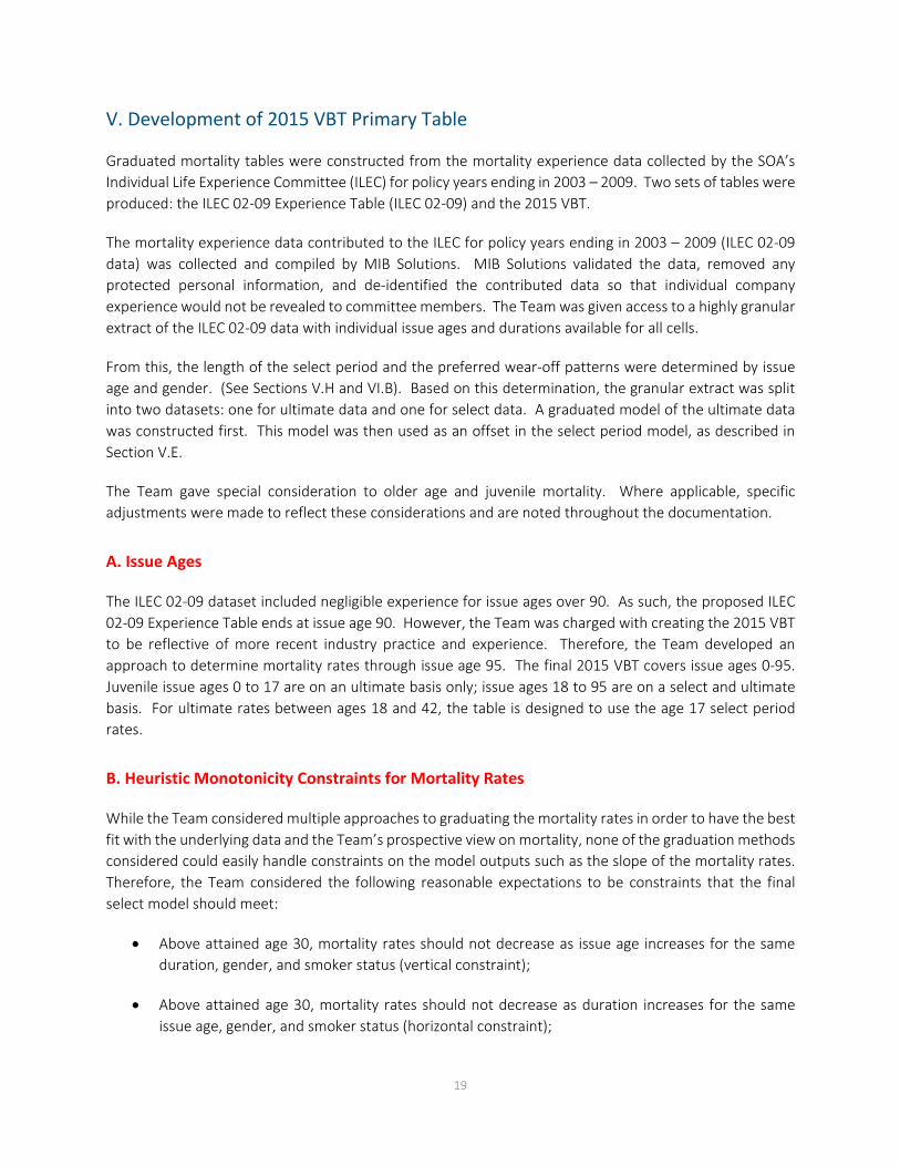
A. Issue Ages

The ILEC 02-09 dataset included negligible experience for issue ages over 90. As such, the proposed ILEC 02-09 Experience Table ends at issue age 90. However, the Team was charged with creating the 2015 VBT to be reflective of more recent industry practice and experience. Therefore, the Team developed an approach to determine mortality rates through issue age 95. The final 2015 VBT covers issue ages 0-95. Juvenile issue ages 0 to 17 are on an ultimate basis only; issue ages 18 to 95 are on a select and ultimate basis. For ultimate rates between ages 18 and 42, the table is designed to use the age 17 select period rates.

B. Heuristic Monotonicity Constraints for Mortality Rates

While the Team considered multiple approaches to graduating the mortality rates in order to have the best fit with the underlying data and the Team’s prospective view on mortality, none of the graduation methods considered could easily handle constraints on the model outputs such as the slope of the mortality rates. Therefore, the Team considered the following reasonable expectations to be constraints that the final select model should meet:

• Above attained age 30, mortality rates should not decrease as issue age increases for the same duration, gender, and smoker status (vertical constraint);

• Above attained age 30, mortality rates should not decrease as duration increases for the same issue age, gender, and smoker status (horizontal constraint);

20

• Mortality rates should not decrease as duration increases for the same attained age, gender, and smoker status (diagonal constraint);

• Mortality rates for males should not be lower than those for females for the same issue age, duration, and smoker status; and

• Mortality rates for smokers should not be lower than those for nonsmokers for the same issue age, duration, and gender.

In certain cases, the Team made adjustments based on their judgment to correct any violations of the above constraints. A listing of all the adjustments is shown in Appendix E.

C. Determination of Graduation Method

There are various graduation approaches which the Team could have used, each with different strengths and limitations. In determining which approach to use, the Team examined three different methods of graduating the data:

1. Whittaker-Henderson (WH);

2. Generalized Additive Models (GAM); and

3. Projection Pursuit Regression (PPR).

Each of the three methods produced models of the composite ultimate data that were smooth and fit the data closely with substantially similar mortality rates at all attained ages up to at least age 95. The Team had chosen an ultimate or omega mortality rate of 0.500. It was necessary to grade from the modeled rate at age 95 to the maximum mortality rate no matter which method was selected. Therefore, any of the three graduation methods examined could have been used on the ultimate data with equal confidence and comfort.

The Team determined it would be advantageous to use the same graduation technique for graduating the select data as for the ultimate data. Preliminary attempts were made to graduate the select data using each of the techniques used for the ultimate data. Based on these efforts, the Team chose to use the GAM approach to graduate the ILEC 02-09 data. While exploration of mortality drivers was cumbersome using the WH approach, the GAM approach allowed the Team to consider potential predictors of mortality other than gender and smoker status in a single model, without overfitting the model to the data as the PPR approach had a tendency to do.

The GAM approach to modelling the ultimate data identified the significant predictors of mortality available in the dataset as gender, attained age, issue age, issue year era2, and face amount band. Due to the fact the overwhelming majority of the ultimate data was from the pre-1980 issue year era for face amounts

2 Groups of issue years generally based on underwriting practices and/or risk classification differences

21

under $10,000, and due to the interaction of issue year era and face amount band as mortality predictors, the Team decided not to include those predictors in the final model. However, the emergence of issue age as a predictor of mortality in the ultimate durations warranted further investigation.

D. Graduation of Ultimate Data

The vast majority of the ultimate data was from policies issued prior to 1980, which was coded as composite due to the unreliability of smoker indications prior to that date. Preliminary analysis was done using the smoker distinct data in the ultimate period from policies issued in 1980 or later. The Team determined that the smoker distinct data in the ultimate period was too thin to use for creating smoker distinct ultimate rates. Thus, the Team decided to ignore the smoker status indications in the ultimate data and treat all of the ultimate data as composite for purposes of graduation and to develop the smoker/nonsmoker distinct rates through development of a three-step process to determine smoker prevalence rates to be applied to the ultimate data. This process included:

a) Extrapolating the select rates into the ultimate period

• For each attained age within each gender and smoker combination, the rates for the last three select durations were used to make an initial estimate of the ultimate rate. The ultimate rate was estimated as the last select rate plus half of the difference between the last select rate and the select rate for the prior duration for that attained age.

• If the increase from the next-to-last select rate to the last select rate seemed unusually large, the ultimate rate was estimated as the last select rate plus the difference between the select rate for the prior duration and the one for the duration before that.

b) Determining the smoker to nonsmoker mortality ratio and smoker prevalence ratio

• The smoker to nonsmoker mortality ratio for each gender and attained age was found by dividing the estimated ultimate smoker rate by the estimated ultimate nonsmoker rate.

• The implied prevalence ratio was determined algebraically to be the proportion of nonsmokers in the ultimate data for which the combination of smoker and nonsmoker data together would result in the composite ultimate rate, given the smoker to nonsmoker mortality ratio.

c) Determining the final Smoker Distinct Ultimate Rates

• The smoker to nonsmoker mortality ratios were smoothed and extended so that the ratio reduced gradually to 100% at age 100 for each gender.

• The prevalence ratios were smoothed and extended to age 100.

• The nonsmoker to composite mortality ratio was then calculated from the smoker to nonsmoker mortality ratio and the nonsmoker prevalence ratio.

22

• The final nonsmoker ultimate rates were then calculated as the composite ultimate rates times the nonsmoker to composite mortality ratios for each gender, and the final smoker ultimate rates were calculated as the nonsmoker ultimate rates times the smoker to nonsmoker mortality ratios.

The issue age effect observed in the data described above was primarily due to a measurable difference between juvenile issue ages and adult issue ages in the ultimate period. Therefore, two separate sub-models were fit to the data: one for juvenile issue ages only (under 18), and one for adult issue ages only (18 and over). Attained age 0 was excluded from the juvenile issue age model and handled separately to avoid causing smoothing anomalies. The Team determined that all juvenile ages and durations should be considered ultimate, while the youngest adult issue ages exhibited a 25-year select period for males and a 20-year select period for females. Therefore, for attained ages 35 and under, the juvenile issue age GAM model was used for the final ultimate composite model. For attained ages 45 and over, the adult issue age GAM model was used for the final ultimate Uni-smoke model. For attained ages between 35 and 45, the two models were connected by log-linear interpolation.

Aggregate mortality rates for males and females were deemed credible through attained age 95; however, experience data for the oldest attained ages was insufficient to determine mortality rates. Therefore, the Team considered additional data sources and reviewed published papers, developed outside the VBT Team, in order to formulate an opinion as to a reasonable level of ultimate mortality rates for the advanced ages.

The most recent payout annuity experience and population mortality data was examined relative to the 2002-09 experience data. The population data sources included the Social Security Administration (SSA), National Center for Health Statistics (NCHS), Human Mortality Database (HMD), Veteran’s Administration (VA), and Canadian Institute of Actuaries (CIA). The review of each of the sources showed that the raw ultimate data appeared less consistent beginning at approximately age 95, the last age at which the ILEC 02-09 experience was sufficiently credible.

Two relevant papers, presented at the 2011 SOA Living to 100 Symposium, were reviewed by the older age subgroup, “Mortality Measurement and Modeling Beyond Age 100” by Natalia S. Gavrilova and Leonid A. Gavrilov* and “Mortality Rates at Oldest Ages” by R.C.W. “Bob” Howard, FSA, FCIA**. The Gavrilova/Gavrilov paper suggested that under-reporting of deaths at the extreme ages (the reasons for this are outlined in the paper) may be causing what appears to be more of a deceleration in mortality rates at these extreme ages than what truly exists. The Howard paper demonstrated mortality rates approaching 0.650 for males and 0.500 for females for Canadians aged 107-110 in the early 2000s, but the data was limited and not fully credible.

* https://www.soa.org/library/monographs/life/living-to-100/2011/mono-li11-5b-gavrilova.pdf ** https://www.soa.org/library/monographs/life/living-to-100/2011/mono-li11-5b-howard.pdf

23

The Team decided to move the ultimate mortality rate from the 0.450 used in the 2008 VBT to 0.500 for this table. The primary reasons for this change were:

(1) the papers implied a higher ultimate mortality rate than the 0.450 used in the 2008 VBT;

(2) while the papers implied an ultimate rate of over 0.500, the data wasn't completely credible and the Team was not comfortable going higher than the 0.500 at this time,

(3) if the omega mortality rate was not changed, the Team was concerned some might believe the 0.450 was the right number because it was also used in the prior table (2008 VBT), and

(4) while some will argue that 0.500 is also not likely the correct number, the Team believed it to be closer to the right number than 0.450.

The main concern was whether a change should occur without sufficient credible supporting information, but the Team believed the listed considerations were sufficiently strong to increase the rate to 0.500 beginning at attained age 112 for both males and females.

Since the aggregate mortality rates for males and females were deemed credible through attained age 95, a process was used to connect and smooth from the attained age 95 mortality rate to the ultimate rate of 0.500. To determine the process to employ, the Team analyzed three different options of a cubic polynomial curve:

A) Fit the curve using the final aggregate GAM model q’s for attained age 93, 94, 95 and 0.500 at attained age 112, 113

B) Fit the curve using the final aggregate GAM model q’s for attained age 93, 94, 95 and 0.500 at attained age 110, 111

C) Fit the curve using the final aggregate GAM model q’s for attained age 93, 94, 95 and 0.510 at attained age 112, 113

After review, the Team determined the best option was to use the cubic polynomial curve fit using the final aggregate GAM model q’s for attained ages 93, 94, 95 and 0.500 at attained ages 112 and 113.

E. Graduation of Select Period Data

Due to concerns about higher mortality on small face amount policies potentially causing the raw experience rates to be too high relative to the experience that we are trying to model, the Team considered excluding certain select period experience on policies with face amounts under $50,000 issued since 2000 to adults under age 70 with lower thresholds for exclusion for issue ages 70 and up and for earlier issue year eras. However, when the Team refit the GAM model by amount with the revised exclusion for small face amount policies and also refit the model with no exclusions, the two models were not materially different, so the Team decided to use the experience on policies of all face amounts in the select period model, with no exclusions.

24

The GAM approach identified gender, smoker status, issue age, duration, face amount band, and issue year era as significant predictors of mortality. The Team fit a GAM model using all of these predictors and found the fit of the model to the data to be very good.

However, upon inspection the Team found numerous violations of heuristic monotonicity constraints in the model and noted that making adjustments to the model to correct these violations could easily create new violations of other constraints due to the complexity of the model. Furthermore, it would be tedious to make manual adjustments due to the number of monotonicity violations identified in the model.

The Team also noted that it would be challenging to present the model with all of these predictors included. Using the traditional issue age and duration grid to display the mortality rates would require 96 such grids to display every combination of gender, smoker status, issue year era, and face amount band. As previously noted for the ultimate rates model, the interaction of face amount band and issue year era as mortality predictors made the model difficult to understand. Therefore the Team decided to eliminate issue year era and face amount band as predictors in the final model.

Exposures and claims for issue ages greater than 90 and for attained ages greater than 105 were excluded from the select period dataset that was fit with a GAM. The amount of exposure and claims excluded was immaterial. The crude model for the select mortality rates was constructed by using the attained age mortality rate from the composite ultimate model by gender as an offset and using the GAM approach to model the relative difference between the actual claims amount and the expected composite ultimate claims amount by issue age and duration separately for each combination of gender and smoker status.

F. Adjustments to the Crude Select Model

Once the crude select period mortality rates were developed via the GAM modeling approach, the Team identified several areas where there were violations in the heuristic monotonicity constrains or which warranted further review and potential adjustment so that the mortality rates were a better reflection of more recent period mortality experience, including:

1. Young Adult Issue Ages

The Team found the crude select model mortality rates for male young adult issue ages appeared to be too low in comparison to the raw experience. A smooth set of adjustment factors was developed for male nonsmokers, issue ages 18 to 31, durations 1 to 15, and another smooth set of adjustment factors was developed for male smokers, issue ages 29 to 36, durations 1 to 7. The resulting rates were checked again to make sure that all heuristic monotonicity constraints were met.

2. Older Issue Ages

The Team expressed concern that the select mortality rates from the crude select model adjusted to meet heuristic monotonicity constraints were too high at issue ages 70 and above for male nonsmokers in comparison to the raw ILEC 02-09 experience data and in light of other privately compiled data from industry and third party consultant studies over similar time periods of exposure. The Team made adjustments to the rates for male nonsmokers, issue ages 70 to 90, durations 1 to 10, and to the rates for

25

male smokers, issue ages 61 to 81, durations 5 to 14. A number of other adjustments were needed in order to meet the heuristic monotonicity constraints. The final rates in the proposed ILEC 02-09 experience table were deemed to provide a reasonable balance between the raw experience data and prior estimates of these rates, given the need for a smooth transition from select to ultimate rates and the relatively small number of claims underlying the raw experience data.

The final smoker distinct ultimate rates were appended to the select smoker distinct rates. Select smoker distinct mortality rates for attained ages 88 to 99 were adjusted to join smoothly with the ultimate smoker distinct mortality rates at these ages. The resulting tables by gender and smoker status are proposed as the ILEC 02-09 Experience Table.

G. Adjustments to move from ILEC 2002-09 Experience Table to 2015 VBT

In order to move from the ILEC 02-09 Experience Table to the 2015 VBT, four additional adjustments were applied:

1. Mortality improvement;

2. Shift in preferred business prevalence;

3. Removal of post-level term anti-selective mortality; and

4. Extension to issue age 95.

1. Mortality Improvement

The Team developed a table of mortality improvement rates by attained age and gender to reflect the recent historical change in mortality rates. These annual improvement rates were converted to monthly improvement factors, which were compounded for 100 months and applied to bring the proposed 02-09 Experience Table rates from the midpoint of the experience (3/1/2006) to the middle of the proposed year of the VBT (7/1/2015). See Section J.

2. Shift in Preferred Business Prevalence

Throughout the experience period, the proportion by amount of business written in preferred underwriting classes shifted to a higher level. The Team developed a set of factors by issue age, duration, and gender to estimate the effect of this shift on future mortality. These factors were applied after the mortality improvement factors. See Section H.2 for further discussion.

3. Removal of Post-Level Term Anti-selective Mortality

The Team examined the underlying ILEC 02-09 experience data and found evidence that some contributed data included experience from level premium term policies that were past the level premium period (durations 11 and later were impacted). Such policies have anti-selective mortality that is much higher than for other types of policies. Since actuaries use separate factors for post-level term exposures when pricing or valuing business, the VBT should exclude this experience. Thus, the

26

Team decided an adjustment should be made to remove the impact of these policies on the results. The analysis outlined below was used to determine adjustments to account for the impact of this post level term anti-selective mortality data.

• The 2004-2009 contributions from all companies and all face amounts were used. The experience was split by gender, issue age, and smoker status.

• First, the actual to expected ratios and exposures by duration for all plans were calculated based on the 2008 VBT.

• Next, the actual to expected ratios and exposures by duration for level premium term plans were calculated based on the 2008 VBT.

• The percentage of the total exposure for durations 11 and later from level premium term plans was calculated.

• The actual to expected ratio was re-calculated, removing the impact of the policies in the post level premium period.

Finally, the ratio of the experience without the post-level premium term plans to the total experience was determined. These final ratios are the adjustment to be made to account for the impact of term policies past the level premium period. The adjustment varies by duration and issue age. The final adjustment is based on the male, nonsmoker experience. Because of the small amount of data and the inconsistencies within the data for the females and smokers, the ratios derived from the male nonsmoker, and shown in the table below, were also applied to male smoker, female nonsmoker and female smoker.

Table 5.1 - Adjustment Factors to Remove Impact of PLT Anti-selective Mortality Issue Ages Durs 11-15 Durs 16-20 Durs 21-25 Durs 26+

18-24 99.9% 99.3% 99.9% 99.2% 25-29 98.7% 99.6% 99.7% 97.4% 30-34 96.5% 98.8% 99.9% 98.1% 35-39 97.0% 99.3% 99.8% 98.1% 40-44 97.5% 99.2% 99.8% 99.4% 45-49 97.5% 98.4% 99.7% 100.0% 50-54 96.1% 97.1% 100.0% 100.0% 55-59 98.3% 99.1% 99.9% 100.0% 60-64 99.1% 99.6% 99.9% 100.0% 65-69 95.7% 99.8% 100.0% 100.0% 70-74 99.4% 100.0% 100.0% 100.0% 75-79 99.8% 100.0% 100.0% 100.0% 80-84 100.0% 100.0% 100.0% 100.0% 85-89 100.0% 100.0% 100.0% 100.0%

Since these factors were not smooth from one issue age and duration group to the next, the factors near the edge of each group were adjusted to provide a smoother transition from one group to the next. These factors were applied after the mortality improvement and shift in preferred business factors.

27

4. Extension to Issue Age 95

Exposures and claims for issue ages greater than 90 and for attained ages greater than 105 were excluded from the select period dataset that was fit with a GAM. The data was sparse and of questionable accuracy for the excluded ages. Ultimate mortality rates beyond age 95 were excluded as questionable patterns were observed at the oldest ages, possibly due to under and late reporting of deaths at the oldest ages, when compared to payout annuity and SSA population data. In the more recent years since the observation years for which data is included in this study, the life industry has significantly improved its procedures in this area. The total amount of exposure and claims excluded was trivial.

The table was extended to provide rates for issue ages past 90 (the limiting age in the 2008 VBT). Mortality rates were included for the first time for issue ages 91-95, as there has been notable, although still limited, increases in production at those ages. The 2015 VBT table was extended to issue age 95 by calculating the ratios of duration 1 mortality to ultimate mortality for issue ages 80 to 90 for each gender and smoker status combination. These ratios were then extended to the higher issue ages using an approximate quadratic extension. One additional rate for issue age 91, duration 3 was estimated by judgment for each gender and smoker status combination, and the remaining select rates were filled in by linear interpolation along the attained age diagonals.

The Team re-performed the heuristic monotonicity checks after the four adjustments and, where necessary, made minor changes in order to remove any violations of the constraints.

H. Determination of Select Period

The length of the select period was analyzed through data submitted for use in the construction of the 2015 VBT to the SOA ILEC. Additional older age data was provided from both Milliman and Towers Watson (now Willis Towers Watson) from their proprietary studies to augment and provide a reasonability check to the SOA submissions. The Team extended the core age data with an appropriate transition to the extreme ages at both the juvenile and older age ends of the spectrum. For purposes of this analysis, ages 18 to 69 were defined to be the core ages; issue ages younger than 18 were considered juvenile and issue ages 70 and above were considered older age.

The Team initially considered issue age, gender, and smoking status as the variables to consider in setting the select period. Ultimately, however, only issue age and gender were used in setting the select period based on anomalies in the results at older ages and changes in smoking cessation rates over time that were embedded in the underlying data. In analyzing the older age business, the raw experience indicated that for males the select period for smokers was longer than for nonsmokers at the older ages, while that of female smokers was shorter than for nonsmokers. Mainly due to the limited exposures of smokers at these ages, the Team decided that the smoker experience was not sufficiently credible to directly use the results of the experience.

Two different underwriting paradigms were also considered: those policy sizes generally deemed to obtain “full” underwriting defined by age and amount criteria and those generally deemed to obtain somewhat less underwriting. As a rough guideline, this can be thought of as policies of $100,000 and above falling in

28

the “full” underwriting paradigm for the core ages ($50,000 for the older ages) and those less than $100,000 at the core ages ($50,000 at the older ages) as the more limited underwriting paradigm. This recommendation focuses on the “full” underwriting paradigm.

The Team also considered factors impacting both the length and the relative slope in the data. This was done to determine if there should be any modifications from the retrospective observed data to a forward looking prospective basis. Ultimately, it was decided to set the prospective select period equal to the observed select period from the underlying data.

The slope of the observed data, however, was modified in order to remove anomalies caused by the underwriting paradigm changes that occurred in the issue years contributing to the underlying data. The approach is discussed in much greater detail below.

1. Factors impacting the Length and Shape of the Select Period

The Select Period in the observed data reflects at least four different and distinct product and underwriting eras. Policies issued prior to the early 1980’s were generally written on an aggregate smoking basis. As nonsmoker/smoker distinct policies became the norm, a disproportionate number of nonsmokers replaced their aggregate policies with cheaper nonsmoker rates. This left a preponderance of exposed policies from this era as underlying smoker risks. Policies underwritten from the early-mid 1980s through the early 1990s were generally written on a nonsmoker/smoker basis, without further breakdown into preferred and residual classes. As such, a disproportionate number of the exposed policies from this era are represented by residual nonsmoker and smoker based risks again based on the ability for preferred risks to obtain cheaper coverage than the policies obtained in the 1980s. Finally, the policies underwritten from the mid-1990s forward are dominated by blood-tested preferred underwritten nontobacco risks which exhibit lower overall mortality than the other two groups of policies both through the select period and beyond. The following table summarizes the various underwriting eras underlying the ILEC 2002-09 experience.

29

Table 5.2 – Comparison of underwriting basis and data considerations by issue year era Issue era Underwriting Consideration

Prior to 1980 • Aggregate smoker basis • This experience comprises the bulk of the ultimate data

Early to mid- 1980s • Introduction of Smoker/non- smoker distinct rates;

• Introduction of blood testing

• High replacement activity amongst NS risks

• Anti-selective mortality • High preponderance of SM risks in

underlying data Mid-1980s to early 1990s

• SM/NS distinct rates • Preponderance of experience on aggregate NS or aggregate SM basis

Early 1990s and later • Introduction of preferred underwriting and better utilization of blood profiles

• Move to tobacco/non-tobacco versus smoker/nonsmoker distinction

• High replacement activity amongst Preferred risks

• Anti-selective mortality • Exhibit lower overall mortality than the

earlier generations of policies both through the select period and beyond

Given the combination of the distinct underwriting eras that underlie the exposure data, it is clear that the slope is steeper than what one should expect if a homogenous group of contemporaneously issued policies were maintained throughout the entire period.

It is also given that the observed ultimate mortality rate for a given issue age is higher in the experience than what would have resulted with a group of homogenous preferred risk/tobacco use distinct group of policies followed from issue to the ultimate durations. The relative disparity between a first duration select mortality rate (i.e., derived from a largely defined group of preferred risk nonsmoker users) and the last observed select duration (i.e., derived from a largely defined group of aggregate/residual tobacco users), implies there are forces affecting both the length and slope of the select period.

While a case could have been made to both shorten and lengthen the length of the prospective select period, the conclusion of the Team was to leave the length of the select period equal to the observable select period for this table, which will be used on a prospective basis. For completeness, the arguments for both lengthening and shortening the select period are stated below.

a) Observable Select Period

The initial cut of data included data with policy anniversaries from 2002 through 2007. This data was analyzed on both a count and an amount basis in order to look for the best indication of the wearing off of underwriting versus being overly influenced by fluctuations due to the size of any particular claim.

In order to look at blocks of business that represented the same general socio-economic group over time, face amounts in excess of $100,000 for durations 1-15 and $50,000 and up for durations

30

of 16+ were analyzed which represented the “full” underwriting paradigm. Policy sizes below these cut points were also analyzed in order to approximate the effect of the less than full underwriting paradigm.

The following approach was undertaken:

1. Working at the gender/smoking status level, the Team split the actual to expected ratios by quinquennial attained age groups and duration using the 2008 VBT ultimate table as the expected. The intent was to balance the scarcity of data while minimizing the amount of interpolation in trying to extend the A/Es to all ages.

2. These raw relationships were then smoothed in two dimensions (age and duration) using a claim weighted Whittaker-Henderson methodology. This approach was used to limit the effect of both the higher ages and the later durations which were overly volatile due to limits in number of claims in these cells.

3. The smoothed results for the quinquennial ages were then interpolated to get all individual attained ages.

4. On an attained age basis, the ratios by duration showed how the experience changed relative to the same expected.

5. From this result, the Team converted the attained age results to an issue age basis by calculating the durational ratios using the attained age A/Es.

6. Once the ratios were calculated by duration, the Team put them into the corresponding issue age / duration cell structure.

7. Finally, the ratio of duration(X)/duration(X-1) was observed to see where the ratios started to decrease. The Team worked under the presumption that as this ratio approaches 1.00, the end of the select period has been reached.

8. This methodology is heavily dependent on the smoothed results which may or may not be a good representation of the later duration A/Es.

9. This methodology uses extrapolation methods at the oldest ages. The Team considered a number of approaches. The “observable” period at the oldest ages was longer than the Team believed appropriate given a professional “judgment” approach.

From this initial starting point, the older age subgroup then focused on issue ages of 50 and above, while the juvenile subgroup focused on the youngest ages.

In setting the select period for the older ages, the primary focus was the experience of issue ages 50 and higher. Separate analyses were done for each of the gender and smoking status combinations. Data from three sources were reviewed to help develop the select period:

• SOA 2008-09 Report of the Individual Life Experience Committee

• Towers Watson (now Willis Towers Watson) Older Age Mortality Study (TOAMS III)

• Milliman Industry Mortality Study and Analysis (MIMSA II)

31

While there was overlap of some data across all three studies (ILEC, TOAMS and MIMSA), the studies were determined to have sufficient variation to be reasonably representative of independent studies.

Data was aggregated into quinquennial attained age groupings through attained age 99 and analyzed by individual duration for durations 1-5 and quinquennial duration groups for durations 6 and later. To eliminate any potential selection bias in the 2008 VBT table, the ultimate (as opposed to select and ultimate) mortality of the 2008 VBT was set as the expected basis for the analysis.

Evaluating the results by attained age allowed the Team to more easily examine how long the impact of selection existed for a given age group. The data used included the SOA ILEC data for 2004-2009 policy anniversaries, along with Milliman’s data with 2005-2009 policy anniversaries and Towers Watson (now Willis Towers Watson) data with 2006-2010 policy anniversaries. This data was segmented by gender and smoking status and policy sizes of $25,000 and up (over 469,000 claims), $50,000 and up (almost 308,000 claims) and $100,000 and up (over 162,000 claims). Again this was segmented into policy sizes representing “full” versus less than full underwriting paradigms.

There were also more male claims than female. Even for nonsmokers, data became somewhat less credible at the oldest issue ages during the later durations. Thus, some judgment was required. There was also some variability in the results by cell and some smoothing was required. In general, the observed select period for female nonsmokers was shorter than for male nonsmokers, although the differences declined by issue age.

The juvenile subgroup’s recommendation was that underwriting for juveniles is sufficiently different from young adults to justify not having a smooth transition in select periods between juveniles and adults. Therefore, there is a "hard underwriting break" in the results due to lack of smoker/nonsmoker distinctions. The juvenile subgroup failed to detect any appreciable select mortality in the data. Even though there is a discontinuity between the juvenile and young adult ages, the amount of selection that occurs in the youngest adult ages is generally viewed to be small on a relative basis, and a true discontinuity doesn’t actually materialize as the juveniles smooth into the unknown smoking adult table. See further discussion in Section I – Further Considerations for Juvenile Ages.

In addition, it was not automatically assumed that the select period for smokers and nonsmokers was the same. A separate review of the select period for smokers was undertaken. First, the appropriateness of using the experience observed select period as a basis for the select period of a newly underwritten block of business was researched. This work focused on the historical changes in smoking prevalence over time and smoking cessation patterns. There are two distinct smoking cessation patterns:

1) Individuals tend to stop smoking as they get older. This is expected to be a recurring pattern occurring in both historical and current environments.

32

2) The level and pattern of smoking cessation has changed over time and is different in today’s environment than in the past. There has been a large societal reduction in smoking prevalence for individuals of specific ages. This change in pattern will impact ultimate smoking mortality.

Smoker mortality rates will tend to be higher than they otherwise would be when there is no societal decrease in smoking prevalence. Historical insured life smoker mortality has been reduced because of the large reduction in societal smoking. This is due to better mortality from those individuals who were smokers at the time that a policy was issued, but have since quit. In addition, the Team also noted that the impact of smokers quitting can lead to lower rates of mortality in future years for policies initially classified and issued as smokers. This is important because there has historically been a high rate of smoking cessation. However, the rate of smoking cessation has declined in recent years.

If the future rate of smoking cessation continues to decline, future smoker mortality rates will be higher than if the historical rates were to continue and smoker mortality will not have the benefit of their improved mortality over time. Some of the quitters, but not all, may have converted their policies to nonsmoker policies. As the additional mortality related to smoking wears off, this could lead to lower mortality rates for those quitters that do not convert and lead to what may appear as a longer select period. The end conclusion is that the reduction in societal smoking cessation will likely increase smoker mortality at the later durations than what it would have been otherwise. This will also increase the select period for smokers.

The second issue the Team considered was the credibility of the experience due to the much more limited amount of smoker experience. Smoker distinct policies became common in the 1980s and all policies issued before that time period do not give credible smoker mortality information. There are two reasons for this. The amount of sold business categorized as smokers is very limited. Also, there are significant data issues with this business as the industry learned how to appropriately classify the smoking status of this business in its databases.

The raw experience indicated that for males the select period for smokers is longer than for nonsmokers at the older ages, while that of female smokers was shorter than nonsmokers. Mostly due to the lack of business issued, the Team did not feel confident that the experience was sufficiently credible to directly use the results of the experience. Therefore, it was decided to use the same select period for smokers and nonsmokers.

b) Argument to Lengthen the Select Period

An argument can be made that the higher ultimate mortality rates would lengthen the observable select period relative to the select period of newly issued business because it will take longer to grade up to the higher ultimate level. However, the select period mortality has been subject to the same environmental forces as the ultimate mortality as one gets to the later select durations towards the end of the observable select period. So while the ultimate level is too high for more contemporarily underwritten policies, the durations approaching ultimate are also increasingly too high as one approaches the end of the select period. It can be argued that, while the level of the later durations and slope of the curve are not appropriate for newly issued business, the change in

33

the mix of business and anti-selective lapsation may not have lengthened the observed select period relative to what would be expected for newly underwritten business.

The Team identified two main arguments for lengthening the select period for newly issued business versus what is in the observable data:

1) Underwriting today gathers more information about the applicant than was collected on policies driving the experience towards the end of the observable select period. Much of the additional information is due to blood testing, which was introduced initially for HIV testing but later became a key driver in the introduction of preferred products into the marketplace. Over time, there has been an increase in the number of standard lab tests conducted on blood samples, thus giving underwriters information about the applicant's health, irrespective of preferred criteria, that was not available previously. In addition, new tests are being added such as elderly questionnaires, prescription profiles, etc. that provide more medical information than was previously available. This additional information should lead to a longer select period than what is currently observed as medical impairments can be identified at earlier stages leading to an overall improved average health for standard risks and a delay in the onset of medical impairments.

2) We know that for business issued in the pre-preferred, smoker-distinct era and aggregate-smoker era there were lives that would be deemed "preferred" if today's preferred structures had been in place when those policies were issued. Recent ILEC emerging experience shows that "preferred-ness" wears off over a longer period than underwriting selection. However, if the business was followed on a non-preferred basis, the observable select period would be a blending of both the preferred and underwriting wear-off. Because of the heavier lapsation of the better risks who could, after their initial policy issue, apply for smoker distinct and later preferred risk class products, the lives remaining in the later durations would be more heavily weighted towards "residual" lives. This shift in the mix of business could make the observable select period shorter than what it would have been if the block had remained intact with an average mix of healthier and residual lives through the entire study period.

c) Argument to Shorten the Select Period

Individual life insurance policies sold on a preferred plan structure became popular in the early 1990s. Due to the lower premium rates for the better risks, the proportion of life insurance on a face amount basis sold to the better risks increased. This is a phenomenon similar to the one that occurred between smokers and nonsmokers when that structure was introduced. The select period of preferred risk classes is longer than that of traditional underwriting. However, unlike smoker and nonsmoker policies, the experience of all risk classes is still grouped together. This grouped experience will show a select period that is actually the combination of two different types of select period. The traditionally defined select period for underwriting to determine standard and substandard risks will be shorter than the overall observed select period in the experience. More importantly, the composition of ultimate experience is composed of generally poorer risks than what composes early duration experience. The question is whether the select period grades

34

off in the same timeframe to a lower (more consistent) ultimate rate or if the lower expected ultimate rate is graded into more quickly.

As discussed above, the Team believed the slope of the observed select period mortality had been affected by the changes in products and underwriting processes that occurred for policies issued that contributed to the underlying data. Primarily among these is the introduction of smoking distinct and preferred underwriting class products. In addition, as 10-year products contribute data beyond the level term period, there are implications of post-level term that need to be taken into consideration.

2. Underwriting Class Slope Impacts

In order to analyze the impact of changing underwriting class structures through time, the following algorithm was utilized.

a. The 2004-2009 contributions from all companies and for all face amounts was segmented by exposures and claims (by amount) into the following categories:

i. Preferred NS (or NT) – Includes all preferred classes ii. Aggregate NS (or NT) - Includes policies issued as smoking distinct but not preferred iii. Residual NS (or NT) – Includes only the worst standard class for preferred distinct policies iv. Composite – Issued on an aggregate smoking status basis v. Preferred SM (or T) – Includes all preferred classes vi. Aggregate SM (or T) - Includes policies issued as smoking distinct but not preferred vii. Residual SM (or T) – Includes only the worst standard class for preferred distinct policies

b. The data was segmented by:

i. Issue Age (18-29, 30-39, 40-49, 50-59, 60-69, 70-79, 80+) ii. Gender iii. Duration (1, 2, 3, 4-5, 6-10, 11-15, 16-20, 21-25, 26+)

c. Appendix H shows the distribution of risk classes listed in subsection a. within each combination of

issue age/gender/duration grouping listed in subsection b. The subgroup was very surprised to see the amount of exposures in the early policy durations attributed to aggregate (non-preferred) NS/SM distinct policies. As a result, the Milliman data used in the MIMSA study was reviewed for comparison purposes. The MIMSA data was much more along the lines expected with very limited exposures for policies issued on an aggregate NS/SM basis. Follow up then occurred with the companies that contributed a preponderance of aggregate NS/SM exposure. Details are discussed in Appendix I. The Team recognizes this as a shortcoming in the data submission, but do not believe it materially distorted the results.

d. Each unique combination of items in subsections a and b, above, were then exponentially

interpolated on both a straight equal weight basis, as well as a claims weighted basis, in order to observe the level and shape of the select period by underwriting class. Unfortunately, there was not enough data to produce intuitively consistent results. The underwriting class was not a good enough indicator to understand relative differences in either early or later durations.

35

e. Next, the data was reviewed to try to determine how the experience might look different going

back in time if the current mix of preferred business had been sold. In the more recent eras where preferred class structures are more prevalent, insureds with better expected mortality tend to buy more and bigger policies which over time improves the overall experience. Going forward, we would expect the experience in later durations to look better than it has historically as the mix of preferred business in the later durations begins to look more like the mix in recent (and presumably future) years.

f. For this additional analysis, the data shown in Appendix H was combined into three groups: "Preferred Era" included a combination of the preferred and residual classes to get the overall mortality when a preferred structure is in place; "Aggregate" included the non-preferred data in the study; and "Total” included the combination of the other two groups. For each group, the mortality rate was calculated by smoking status, gender, age and duration as shown above using the claims and exposures for each group.

g. The ratios of the "Preferred Era" mortality and the "Aggregate" mortality were calculated relative

to the "Total" mortality. These ratios gave us relationships over time between the "Preferred Era" and "Aggregate" mortality. The resulting ratios were then linearly interpolated on a claims weighted basis to get smooth relationships.

h. In the ILEC 2002-09 Study, about 64% of the duration 1 business was categorized as having a

preferred class structure. The ratios calculated in point g were weighted together assuming this was the mix of business in all durations in the study. The resulting combined ratio is an approximation of how much better the experience might have been if the current mix of preferred business had been in place throughout the entire study.

i. The resulting ratios from subsection h were capped at 100% and the age patterns were smoothed,

so the progression by age made sense. The results were reviewed by gender and smoking status. Because of the volatility in the results, it was decided to use the male nonsmoker results for everything. Below is a graph of the recommended factors. The actual factors are shown in Appendix J.

36

Chart 5.1 – Factor adjustments by issue age and duration to account for changing mortality slopes caused by data from differing underwriting eras

92.0%

93.0%

94.0%

95.0%

96.0%

97.0%

98.0%

99.0%

100.0%

1 2 3 4 5 6 7 8 9 10 11 12 13 14 15 16 17 18 19 20 21 22 23 24 25

25

35

45

55

65

75

85

37

3. Recommended Select Period Length

The Team recommended using the observed select period to represent the cohort based select recommendation with the adjustments for post level term mortality, changes in underwriting over time and additional older age considerations described above. The select period for the respective issue ages and gender breakdowns are shown in the table below.

Table 5.3 - 2015 VBT Select Period Issue Age

MALE NS & SM

FEMALE NS & SM

Issue Age

MALE NS & SM

FEMALE NS & SM

0-17 0 0 75 15 14 18-54 25 20 76 14 14

55 24 19 77 13 13 56 23 19 78 13 13 57 23 19 79 12 12 58 22 19 80 11 11 59 22 19 81 11 11 60 21 19 82 10 10 61 21 19 83 9 9 62 20 18 84 8 8 63 20 18 85 8 8 64 19 17 86 7 7 65 19 17 87 6 6 66 18 16 88 5 5 67 18 16 89 5 5 68 18 16 90 4 4 69 18 16 91 3 3 70 17 15 92 2 2 71 17 15 93 2 2 72 17 15 94 2 2 73 16 14 95 1 1 74 16 14

I. Additional Considerations for Juvenile Risks

The 2008 VBT report for juveniles made the following recommendations:

For juvenile ages (defined herein as less than 18), the underlying data was sparse and resulted in a pattern of mortality rates inconsistent with a more traditional select and ultimate rate structure. The Team felt a 25-year select and ultimate pattern did not make sense for juvenile risks, based on the level of underwriting generally performed at these ages. The actual mortality experience for male issue ages 0-17, durations 1-10 was roughly 78% of the population mortality; for females, the actual mortality experience was 83%. The aggregate tables used the actual experience for all face amounts for issue age 0, duration 1. Beyond that, juvenile mortality was set equal to 78% of the population mortality for males and 83% for females up to attained age 10. Mortality was then graded between population and aggregate table rates between ages 10 and 25. This resulted in no

38

select period for issue ages 10 and under. The population mortality table used was the 2002 Social Security Administration data projected to 2003.

In light of previous recommendations and the additional mortality data available for 2015 VBT, the juvenile subgroup developed the following objectives and recommendations for juvenile mortality rates for the 2015 VBT:

• Relation to Population Mortality3: Due to the sparse data available, the 2008 VBT Team recommended a flat percentage of population mortality (varying by male and female) for attained ages greater than 0. We reviewed 2002-2009 juvenile mortality experience relative to population mortality in order to determine whether to make a similar recommendation for 2015 VBT.

Recommendation: The Team compared juvenile mortality experience to 2007 U.S. Life Tables and determined that mortality experience varied materially by attained age as a percentage of population mortality. We provided raw juvenile mortality rates to the VBT Graduation Subgroup to develop graduated attained age juvenile mortality rates.

• Select Mortality Analysis: The Team reviewed whether the 2002-2009 data showed any indication of a select and ultimate pattern of mortality or whether to continue to recommend an attained age basis for juvenile mortality (possibly subject to any grading into adult age mortality rates due to smoothness requirements).

Recommendation: Similar to observations from the 2008 VBT development, the Team observed no clear indication of any select versus ultimate mortality rates in the juvenile data, especially when compared to young adult age mortality experience. For the 2015 VBT, the Team recommended that juvenile mortality remain attained age only, with the possible caveat that duration 26 (and greater) mortality may need to be graduated smoothly into adult attained ages, possibly causing some element of select mortality rates for smoothness purposes at higher juvenile issue ages and select durations.

• Mortality Improvement: The Team evaluated juvenile mortality experience to determine whether there is evidence of mortality improvement by experience year for juvenile issue ages.

Recommendation: Due to sparse juvenile data, the Team observed no clear indication of mortality improvement present in the 2002-2009 data different than what was recommended for overall mortality improvement by the Mortality Improvement Subgroup. The Team reviewed analysis of other sources of data studied by the Mortality Improvement Subgroup and the recommendation was to reflect mortality improvement for juveniles consistent with the overall recommendations of the Mortality Improvement Subgroup.

3 United States life tables, 2007. National vital statistics reports; Vol 59 no 9. Hyattsville, MD: National Center for Health Statistics. 2011 (pages 10 and 12).

39

The Team compared the ratio of raw juvenile mortality rate experience to the 2007 U.S. population mortality by attained age as shown in the charts below:

Chart 5.2 – A/E ratio (by Count) by attained ages 0-42, Male risks (E=2007 US Life (population) mortality)

Chart 5.3 - A/E ratio (by Count) by attained ages 0-42, Female risks (E=2007 US Life (population) mortality)

These charts show that juvenile mortality rates did not appear to be a level percentage of population mortality. The Team also noted the unusual spike (particularly for males) around attained age 10 (which is analyzed further in a later set of charts).

40

The Team also analyzed juvenile mortality ratios by face amount as shown in the charts below:

Chart 5.4 - A/E ratio (by Amount) by attained ages 0-42, Male risks (E=2007 US Life (population) mortality)

Chart 5.5 - A/E ratio (by Amount) by attained ages 0-42, Female risks (E=2007 US Life (population) mortality)

Comparing these charts to the mortality ratios by count showed no material evidence of mortality variations by face amount for juveniles.

41

The chart below shows U.S. population rates for attained ages 1 to 17:

Chart 5.6 – 2007 US Life table (population) mortality rates per 1,000 by gender

The above chart show that juvenile 2007 population mortality rates bottom out at or around age 10.

0.0000

0.2000

0.4000

0.6000

0.8000

1.0000

1 2 3 4 5 6 7 8 9 10 11 12 13 14 15 16 17

Mor

talit

y Ra

te P

er 1

,000

Attained Age

Female Male

42

The Team also compared 2008 VBT juvenile mortality rates (which were expressed as a flat percentage of population mortality based on 2002 Social Security population mortality rates) to 2007 U.S. Life Table mortality:

Chart 5.7 – Mortality ratio of 2008 VBT ANB to 2007 US Life Table (population), by gender

This chart shows a similar spike in 2008 VBT mortality in relation to population mortality. Based on these charts, the Subgroup was comfortable that the bottoming out of the 2007 population mortality at or around attained age 10 does not occur (at least to the same degree) in the insured mortality experience.

60%

70%

80%

90%

100%

110%

120%

1 2 3 4 5 6 7 8 9 10 11 12 13 14 15 16 17

Mor

talit

y Ra

tio

Attained Age

Female Male

43

Select Mortality Analysis for Juveniles

There was not enough juvenile data to do a detailed analysis of select mortality experience for the juvenile risks, so the Team grouped juvenile mortality data into "early duration" versus "later duration" blocks by attained age to see if there was any clear evidence of juvenile select mortality. The table and charts below compare mortality ratios by juvenile attained ages, grouping policy durations less than or equal to six versus durations greater than six:

Table 5.4 – Juvenile mortality ratios by attained age and duration group Juvenile Mortality By Attained Age and Longevity Group

Age

Male Actual Male Expected Male A/E Male Select Ratio

Female Actual Female Expected Female A/E Female Select Ratio

Dur <=6

Dur >6

Dur <=6

Dur >6

Dur <=6

Dur >6

Dur <=6

Dur >6

Dur <=6

Dur >6

Dur <=6

Dur >6

ALL 903 4879 1114.2 6053.1 81.0% 80.6% 100.5% 350 1880 507.6 2341.1 68.9% 80.3% 85.9% 6 20 16 43.8 33.2 45.7% 48.2% 94.8% 16 17 33.5 25.6 47.7% 66.4% 71.8% 7 19 31 32.4 42.9 58.6% 72.3% 81.1% 21 17 25.0 33.0 83.9% 51.5% 163.0% 8 8 37 24.9 43.7 32.1% 84.7% 37.9% 11 26 20.5 35.8 53.6% 72.7% 73.8% 9 10 41 18.2 39.5 54.9% 103.9% 52.8% 10 25 17.2 36.9 58.2% 67.7% 86.0%

10 19 47 13.6 34.1 139.5% 137.7% 101.3% 10 40 15.2 37.5 65.9% 106.6% 61.8% 11 17 46 13.7 39.4 124.2% 116.8% 106.4% 12 32 14.9 42.4 80.3% 75.5% 106.4% 12 16 55 21.0 68.7 76.2% 80.1% 95.1% 9 50 17.3 55.4 51.9% 90.3% 57.5% 13 28 83 36.7 132.5 76.4% 62.6% 121.9% 9 47 22.3 79.1 40.4% 59.4% 67.9% 14 30 145 57.4 225.5 52.3% 64.3% 81.3% 12 74 28.7 111.3 41.8% 66.5% 62.9% 15 48 211 79.0 328.9 60.8% 64.2% 94.7% 29 118 35.8 148.3 81.0% 79.6% 101.7% 16 74 310 108.3 430.2 68.3% 72.1% 94.8% 41 166 45.8 183.6 89.4% 90.4% 98.9% 17 143 438 143.7 535.2 99.5% 81.8% 121.6% 54 210 57.2 214.6 94.5% 97.9% 96.5% 18 121 562 137.7 631.5 87.9% 89.0% 98.7% 27 206 50.8 235.7 53.2% 87.4% 60.8% 19 135 617 128.0 722.7 105.4% 85.4% 123.5% 36 206 43.7 250.9 82.3% 82.1% 100.2% 20 112 693 115.2 824.4 97.2% 84.1% 115.7% 23 212 36.8 266.6 62.6% 79.5% 78.7% 21 67 756 91.7 920.9 73.0% 82.1% 89.0% 15 204 27.9 283.5 53.8% 72.0% 74.7% 22 36 791 48.8 999.8 73.8% 79.1% 93.3% 15 230 14.9 300.9 100.5% 76.4% 131.5%

44

Chart 5.8 – A/E Mortality Ratios by Duration Juvenile Issue Ages, Male Risks

Chart 5.9 – A/E Mortality Ratios by Duration Juvenile Issue Ages, Female Risks

Chart 5.10 – Ratio of select mortality durations 6 and later to duraitons 1-5, juvenile issue ages, male risks

Chart 5.11 – Ratio of select mortality durations 6 and later to durations 1-5, juvenile issue ages, female risks

45

Grouping by different durations (e.g., 5, 7, etc.) showed similar results. While the data may indicate some pockets of select mortality (males under 10, early teen females and females overall on average), death claims were sparse at many attained ages, even after grouping. So the team felt that there was no clear overall pattern of any significant select mortality for juveniles and recommended continuation of attained age rates for juveniles.

The only caveat to the “attained age only” recommendation was to question whether some degree of variation by attained age was needed to grade into adult age mortality (similar to what was done in 2008). We also looked at young adult mortality ratios by duration grouping to compare the results to juveniles:

Chart 5.12 – A/E mortality ratios by duration group and attained age Issue ages 18-24, Male risks

0.0%

20.0%

40.0%

60.0%

80.0%

100.0%

120.0%

24 25 26 27 28 29

Ratio

Attained Age

Durations <=6 Durations >6

46

Chart 5.13 - A/E mortality ratios by duration group and attained age

Issue ages 18-24, Female risks

Chart 5.14 - Ratio of select mortality durations 6 and later to duraitons 1-5 by attained age Issue ages 18-24, Male risks

0.0%

20.0%

40.0%

60.0%

80.0%

100.0%

120.0%

24 25 26 27 28 29

Ratio

Attained Age

Durations <=6 Durations >6

0%

20%

40%

60%

80%

100%

24 25 26 27 28 29

Ratio

Attained Age

Select Ratio Pre to Post Duration 6Issue Ages 18-24 Male

47

Chart 5.15 - Ratio of select mortality durations 6 and later to duraitons 1-5 by attained age Issue ages 18-24, Female risks

These charts show that, unlike juveniles, there is a distinct select mortality element in young adult ages. This appeared to confirm that juvenile policy and underwriting characteristics are distinctly different such that no smoothing between juveniles and adults is called for at select durations of the mortality table. There still perhaps could be reasons to smooth and adjust ultimate duration (26+) mortality rates for practical considerations should there be significant discontinuities in ultimate mortality experience. The Juvenile Subgroup recommended leaving this question for the graduation team to address in developing final attained age mortality rates.

J. Mortality Improvement

The Team analyzed mortality improvement in two segments, first from the mid-point of the exposure period to the end of the exposure period, and then from the end of the exposure period to the mid-year of the start date of the table, July 1, 2015. The Mortality Improvement Subgroup was tasked with reviewing recent mortality improvement levels based on available data for both the insured and general population to determine the appropriate improvement factors, if any, to use for both segments.

As a result of this work, the Subgroup recommended a set of improvement factors that vary by gender and attained age to be used in conjunction with the 2015 VBT. These factors are found in Appendix L.

For the Period 2002-2009:

For this period, the actual general population improvement data was known; therefore, the Team recommended developing and applying actual mortality improvement factors to adjust each experience year through 2009.

0%

20%

40%

60%

80%

100%

24 25 26 27 28 29

Ratio

Attained Age

Select Ratio Pre to Post Duration 6Issue Ages 18-24 Female

48

For the Period 2009-2014:

For this period, the Team recommended applying average annual improvement rates that vary by gender and by attained age and to be based on general population data produced by the Social Security Administration (SSA). The Team recommended setting these rates equal to the arithmetic average of:

1) the average annual improvement rates implied by the SSA’s most recent intermediate level projection of mortality for the Social Security population (2010 Trustee’s Report), which was the last published Trustees report at the time of the analysis; and

2) the actual historical average annual improvement rates implied by SSA data for the most recent 10-year period available (1997-2007).

The Team considered the following in developing the recommendation:

• A desire for the methodology to weight the impact of recent historical rates of improvement with a longer-term assumption (SSA intermediate projections) in determining projected improvement rates. This approach is (at a very high level) consistent with the current Continuous Mortality Investigation (“CMI”) projection models, which basically project rates based on past experience, but trend toward a long term assumed average annual improvement level.

• For the common company data from the ILEC 2002-09 study, the individual life insurance mortality was initially examined only for policies in the ultimate period. The Team decided that given the relatively short period over which the historical insured experience is available, and given the year over year volatility of results (likely in part the result of both industry impacts as well as changes in underlying mortality rates), general population data was the preferable source for determining an applicable improvement scale for use in the VBT table development effort.

• For the general population data source, the subgroup examined several sources of general population data including the U.S. Vital Statistics data, the Human Mortality Database (HMD), and the SSA data. The SSA data was selected as the source for general population analysis for several reasons, including the fact that it is one of the more strongly vetted sources, that it may have better data regarding age at death for the oldest ages than HMD, and that it includes projections of future estimated mortality.

• In addition to the data sources discussed above, the Subgroup also researched and considered additional factors with potential to impact mortality improvement experience. These included gender, attained age, smoker status, socioeconomic status, and differences in cause of death between the insured and general population. In most cases, sufficient data was not available to allow for development of adjustments to mortality improvement estimates for these factors.

49

Attained Age

Mortality improvements have historically varied materially by attained age group. This was consistent in the data analyzed. The resulting recommendation provides for variation in improvement rates by attained age.

Gender

In the data analyzed, male mortality improvement rates have historically been greater than female mortality improvements. However, the Team observed evidence that differences have been reducing in recent years. The recommendation provides for variation in improvement rates by gender.

Smoking Status

The Mortality Improvement Subgroup also looked at smoker status as a driver of mortality improvement. The Subgroup examined numerous studies that examined differences in base mortality by smoker status; however, there were far fewer sources available that track mortality rates, split by smoking status, over a sufficient number of years to estimate improvement differences. For example, the two population datasets the subgroup primarily looked to (SSA data and HMD data) were not split by smoker status. Existing insured population mortality improvement scales do not vary by smoker status; and mortality improvements used in the development of prior VBT tables did not vary by smoker status, mostly due to lack of credible data.

Insurance population mortality studies do track mortality data by smoking status and the 21 Common Company ILEC data for years 2002 to 2007 (the initial data period in the ILEC study before the two additional years, 2008-2009, were added) provided data for four years of annual mortality improvement. The SOA’s Global Mortality Improvement study used the same data and did recommend a variation in future mortality improvement assumptions by smoking status. However, due to the relatively short period over which the 2014 future mortality improvement scale will need to project experience, combined with the small amount of data available, the Subgroup concluded there was insufficient basis for recommending a variation by smoking status.

Socioeconomic Status

Several sources of data related to differences in mortality improvement by socioeconomic status were examined, including academic studies based on general population results, as well as the common company insured population data from 2002-2007 using face amount band as a proxy for income/economic status. There is evidence that both base mortality and mortality improvement are more favorable for segments of the population in higher socioeconomic categories, whether determined by income, wealth or education level. However, due to the shorter time periods over which data from both industry and academic sources are available at this point in time, it was decided that for VBT table development purposes, we do not recommend an adjustment to estimated improvement levels by socioeconomic status.

50

Differences in Cause of Death (Insured versus General Population)

Another potential source of variation in mortality improvement levels stems from differences in the underlying cause of death for specific populations. The Subgroup examined general population mortality data and some limited insurance industry data by cause of death in order to determine whether there are significant differences in the sources of mortality results between the general and insured populations. Based on limited data covering the period 2005-2009, we found that a larger percentage of insureds die from cancer than the general population, but a lower percentage of insureds die from cardio/respiratory causes.

The Team then attempted to estimate the impact on improvement levels of differences in mortality by cause. To estimate this, the subgroup first determined the impact on general population improvement levels assuming that the general population experienced the same mix of deaths and the same improvement levels by cause as insureds. This resulted in a potential 0.5% greater average annual improvement rate for insureds over the four year period examined.

However, as with other factors examined, current data was not yet fully credible. Therefore, we recommend that no adjustments to the VBT mortality improvement assumption be made due to differences in cause of death between the insured and general population at this time.

51

VI. Development of 2015 Relative Risk (RR) Tables

In order to determine the relative risk (RR) table mortality rates, the Team needed to determine the number of RR tables, the relativity amongst the tables, as well as the level of preferred wear-off to assume.

A. Number and Relativity of RR Tables

In determining the number of relative risk tables (RR tables), the Team analyzed the range of experience of companies’ nonsmoker classes, as well as the number of claims in each class. The analysis is shown in the chart below. Note, the analysis was performed prior to the VBT table being projected one additional year from 2014 to 2015 and was only performed for companies with three or more non-tobacco risk classes. The 2015 VBT expected basis was adjusted to remove improvement to midpoint of data period for each company.

Chart 6.1 – Distribution of A/E ratios by number of claims

Nonsmoker risks

As shown, there was significant variation in experience across the contributing companies. By amount, the actual to expected ratios ranged from 36% to 1,164% for nonsmoker risks and from 41% to 194% for smoker risks. By policy count, the actual to expected ratios ranged from 49% to 863% for nonsmoker risks and from 75% to 184% for smoker risks. In some cases, the lowest A/E ratio was not always for a company’s best preferred risk class.

The Team decided to keep the number of RR tables the same as the 2008 VBT; however, based on the observed experience, the Team determined the relativity should differ from what was in the 2008 VBT. The resulting RR tables are RR 50, RR 60, RR 70, RR 80, RR 90, RR 100, RR 110, RR 125, RR 150 and RR 175, where the RR 100 is the same as the VBT Primary Nonsmoker Table.

02468

101214

Num

ber

of c

ompa

nies

A/E where E=2014 VBT

Range of A/Es for all NS risk classes by number of claims

50+ Claims25-49 Claims<25 Claims

52

To determine the relative risk tables for the smoker risks, there was very limited data to justify a different structure or relativity from that in the 2008 VBT. Therefore, the smoker RR tables are RR 75, RR 100, RR 125, and RR 150, where the RR 100 is the same as the VBT Primary Smoker Table.

B. Preferred Underwriting Wear-off Pattern

During the development of the 2008 VBT, the 2008 VBT team considered several studies in analyzing the length and shape of the wear off of preferred underwriting. This wear off is separate and distinct to the wear off of general underwriting via the select period. The full discussion can be found in the write-up for the 2008 VBT table, which is reproduced in Appendix G.

The Team analyzed the level of wear-off in the underlying ILEC 2002-09 data, but the experience was still emerging. There was virtually no additional information available from the 2008 VBT analysis, which was extensive. The preponderance of aggregate NS data in early durations further complicated the analysis; therefore, the Team also examined Milliman’s MIMSA study to further inform its judgment regarding the preferred wear-off pattern and level. In the end, the preferred wear-off factors are similar to those for the 2008 VBT with the exception that they grade off to attained age 95, which is the same grade off as the underlying select period, rather than age 90. The factors used to grade from age 90 to 95 were based on professional judgment. The final preferred wear-off factors for select issue ages and durations are shown in the table below: The full set of preferred wear-off factors are shown in Appendix F.

Table 6.1 - Preferred Wear-off Factors for Select Issue Ages and Durations

Issue Age Duration

1 5 10 15 20 25 25 0.0% 0.0% 0.0% 0.0% 0.0% 2.2% 35 0.0% 0.0% 0.0% 2.1% 5.6% 11.4% 45 0.0% 1.8% 5.3% 11.1% 19.3% 29.9% 55 0.0% 5.2% 14.0% 25.2% 39.0% 55.3% 65 0.0% 11.0% 27.4% 46.8% 66.2% 81.4% 75 0.0% 22.8% 51.1% 72.5% 94.3% 100.0% 85 0.0% 27.8% 82.9% 100.0% 100.0% 100.0%

C. Determination of the RR Mortality Rates

The relativity of an RR table indicates the approximate average overall mortality level of the RR table compared to the 2015 VBT Primary Table for the same gender and smoker status. It is not the same as applying a constant factor to the entire table. For example, the average mortality of the 2015 VBT MNS RR 70 Table is about 70% of the average mortality of the 2015 VBT MNS Primary (RR 100) table, but for a specific issue age and duration, the ratio of the RR 70 q[x]+t to the corresponding RR 100 q[x]+t might not be 70%.

53

Because extensive work had been done for the 2008 VBT and new information was insufficient, the mortality rates for the 2015 VBT RR Tables are based on the pattern of mortality rates by issue age in the 2008 VBT RR Tables. For duration 1, preliminary 2015 VBT RR mortality rates were calculated by multiplying the 2015 VBT Primary (RR 100) Table mortality rate times the ratio of the corresponding 2008 VBT RR mortality rate to the 2008 VBT Primary (RR 100) Table mortality rate at the same issue age.

(1) 𝑞𝑞[𝑥𝑥]15 𝑅𝑅𝑅𝑅 𝑛𝑛𝑛𝑛 = 𝑞𝑞[𝑥𝑥]

15 𝑅𝑅𝑅𝑅 100 ∙𝑞𝑞[𝑥𝑥]08 𝑅𝑅𝑅𝑅 𝑛𝑛𝑛𝑛

𝑞𝑞[𝑥𝑥]08 𝑅𝑅𝑅𝑅 100

Four of the nonsmoker RR tables for the 2015 VBT did not have a corresponding 2008 VBT RR table. The preliminary duration 1 mortality rates for these RR tables required special handling. We used linear interpolation or extrapolation to derive the duration 1 mortality rates. Specifically, the preliminary duration 1 mortality rates for the 2015 VBT RR 125 tables for male nonsmokers and female nonsmokers were calculated by interpolation using the average of the 2008 VBT RR 120 table and the 2008 VBT RR 130 table.

(2) 𝑞𝑞[𝑥𝑥]15 𝑅𝑅𝑅𝑅 125 = 𝑞𝑞[𝑥𝑥]

15 𝑅𝑅𝑅𝑅 100 ∙�𝑞𝑞[𝑥𝑥]

08 𝑅𝑅𝑅𝑅 120+𝑞𝑞[𝑥𝑥]08 𝑅𝑅𝑅𝑅 130�

2�

𝑞𝑞[𝑥𝑥]08 𝑅𝑅𝑅𝑅 100

The preliminary duration 1 mortality rates for the 2015 VBT RR 175 tables for male nonsmokers and female nonsmokers were calculated by extrapolation by proportionately increasing the excess of the 2008 VBT RR 160 tables over the 2008 VBT RR 100 tables.

(3) 𝑞𝑞[𝑥𝑥]15 𝑅𝑅𝑅𝑅 175 = 𝑞𝑞[𝑥𝑥]

15 𝑅𝑅𝑅𝑅 100 ∙ �1 +�𝑞𝑞[𝑥𝑥]

08 𝑅𝑅𝑅𝑅 160−𝑞𝑞[𝑥𝑥]08 𝑅𝑅𝑅𝑅 100�∙75 60�

𝑞𝑞[𝑥𝑥]08 𝑅𝑅𝑅𝑅 100 �

The preliminary duration 1 mortality rates for the 2015 VBT RR 60 and RR 50 tables for male nonsmokers and female nonsmokers were calculated by extrapolation by proportionately increasing the discount of the 2008 VBT RR 70 tables from the 2008 VBT RR 100 tables.

(4) 𝑞𝑞[𝑥𝑥]15 𝑅𝑅𝑅𝑅 60 = 𝑞𝑞[𝑥𝑥]

15 𝑅𝑅𝑅𝑅 100 ∙ �1 −�𝑞𝑞[𝑥𝑥]

08 𝑅𝑅𝑅𝑅 100−𝑞𝑞[𝑥𝑥]08 𝑅𝑅𝑅𝑅 70�∙(100−60)

(100−70)�

𝑞𝑞[𝑥𝑥]08 𝑅𝑅𝑅𝑅 100 �

(5) 𝑞𝑞[𝑥𝑥]15 𝑅𝑅𝑅𝑅 50 = 𝑞𝑞[𝑥𝑥]

15 𝑅𝑅𝑅𝑅 100 ∙ �1 −�𝑞𝑞[𝑥𝑥]

08 𝑅𝑅𝑅𝑅 100−𝑞𝑞[𝑥𝑥]08 𝑅𝑅𝑅𝑅 70�∙(100−50)

(100−70)�

𝑞𝑞[𝑥𝑥]08 𝑅𝑅𝑅𝑅 100 �

For subsequent durations, the ratio used in duration 1 was worn off using the Preferred Underwriting Wear-off Factors by issue age and duration, 𝑊𝑊𝑊𝑊𝑥𝑥,𝑡𝑡 , described above in Section VI.B.

(6) 𝑞𝑞[𝑥𝑥]+𝑡𝑡−115 𝑅𝑅𝑅𝑅 𝑛𝑛𝑛𝑛 = 𝑞𝑞[𝑥𝑥]+𝑡𝑡−1

15 𝑅𝑅𝑅𝑅 100 ∙ �1 − ��1 −𝑞𝑞[𝑥𝑥]15 𝑅𝑅𝑅𝑅 𝑛𝑛𝑛𝑛

𝑞𝑞[𝑥𝑥]15 𝑅𝑅𝑅𝑅 100� ∙ �1 −𝑊𝑊𝑊𝑊𝑥𝑥,𝑡𝑡���

Please see Appendix D for sample mortality rate calculations following the above formulas.

54

An exception to all of the formulas above was made for issue ages 18 to 25 for nonsmokers. For these issue ages, the preliminary duration 1 mortality rates were calculated using the issue age 26 values from the 2008 VBT tables in each of the formulas above. This was done to ensure consistency between smoker and non-smoker tables at higher RR relativities.

After preliminary rates were calculated using the formulas above, two types of adjustments were made to assure consistency within and among these tables.

• First, the ultimate period for the RR tables was checked for consistency with the ultimate period of the Primary table. Mortality rates in the ultimate period of the RR tables were adjusted to be the same for a given attained age. For females, the ultimate rate after wear-off is achieved no later than the 21st duration; for males, the ultimate rate after wear-off is achieved no later than the 26th duration.

• Second, the heuristic monotonicity constraints described above in Section E were applied. The diagonal constraint was applied by formula for all issue ages and durations in the select period by setting each mortality rate equal to the minimum of the rate diagonally above it and the preliminary mortality rate calculated by the formulas above.

(7) 𝑞𝑞�[𝑥𝑥]+𝑡𝑡15 𝑅𝑅𝑅𝑅 𝑦𝑦𝑦𝑦 = 𝑚𝑚𝑚𝑚𝑚𝑚�𝑞𝑞[𝑥𝑥]+𝑡𝑡

15 𝑅𝑅𝑅𝑅 𝑦𝑦𝑦𝑦 , 𝑞𝑞�[𝑥𝑥−1]+𝑡𝑡+115 𝑅𝑅𝑅𝑅 𝑦𝑦𝑦𝑦 �

The vertical and horizontal constraints were then applied to individual cells above attained age 32 manually as needed. The decision was made to begin at attained age 32 instead of attained age 30, which was the lowest attained age for these constraints for the Primary tables, because it appeared that the preferred underwriting adjustments altered the shape of the “accident hump” for the young ages. The adjustments for the vertical and horizontal constraints were made to the fewest cells possible in each case.

D. Use of the RR Tables and Limitations

The Relative Risk Tool (RR Tool) is a calculator developed by the Underwriting Criteria Team (UCT), a subcommittee consisting of underwriters, medical directors, and actuaries. The team members studied actual experience and lab data, and used this and professional judgment to develop the Relative Risk Ratio (RRR) methodology. This involved providing an appropriate relative mortality risk, based on industry averages, for all risk classes of a wide range of preferred risk program structures. The resultant RRR output from the RR Tool is the Relative Risk Score (RR Score or RRS). Separate RR Scores are provided for each risk class in the preferred program structure. For more details, please refer to the “RR Tool - Relative Risk Score Calculator” report on the SOA website, published Nov. 3, 2016.

The range of preferred risk class structure definitions used in the market is very broad. The RR Tool provides reasonable expected relationships based on each individual preferred risk class underwriting program definition. It determines RR Scores and Prevalence of each risk class for any life insurer’s specific preferred risk class program. It is designed to handle various approaches to assigning preferred

55

classes, including the “Knockout” and “Debit-credit” logic approaches. It also accommodates preferred program criteria with elements of both.

The RR Score is the expected mortality before any preferred wear-off of a particular risk class relative to the overall average mortality for all standard (i.e., non-substandard) risks at the same gender, age, smoking status, and duration. The prevalence is the proportion of all standard risks expected to qualify for the particular risk class defined in the preferred structure. Both the RR Scores and prevalences are based on assumptions built into the RR Tool, not on the experience of the particular program. The RR Scores are a good overall industry average starting point for assumptions, in exactly the same vein that the VBT table is a good starting point for the overall mortality.

The use of the word standard must be interpreted very carefully in the context of the RR Tool and RR Score. The highest mortality standard risk classes in a preferred program are often referred to as residual or residual standard. The use of the word standard in a preferred risk program can be confused with the term “standard” in a standard / substandard context. In the first stage of a risk evaluation process, lives are determined (usually by underwriters) to be standard or substandard risks based on the evaluation of the circumstances of each individual life. Only the risks determined to be “standard” risks qualify for a preferred risk programs. The RR Score does not reflect the portion of the portfolio which are deemed to be impaired or substandard risks. All of the preferred risk classes, whether super preferred, preferred, standard, standard-residual or whatever other risk class names an insurer uses are standard underwritten risks.

The RR Score for any particular risk class is the base indicator of the appropriate 2015 VBT RR table to be used in setting its reserves. It represents the average risk of that class. Adjustments can be made during the valuation process due to unique program characteristics.

Table 6.2 –Approximate risk class structure for each RR Table 2015 VBT

(NS – 10 RR Tables) 50 60 70 80 90 100 110 125 150 175 Super Preferred Preferred Standard

The actual risk class experience of many, if not most, insurers will be different than the results from each other and the calculator. The mortality results of the individual life insurers can vary significantly, even when comparing only overall portfolio experience. The credibility of mortality experience of single preferred classes is even lower than for a carrier’s entire portfolio, creating an even wider range of possible outcomes. In addition, experience differences by insurer can occur due to factors other than credibility, including many which are systematic. As with any estimator, there are limitations in the RR Score’s ability to accommodate any program’s overall environment:

• The assumptions have been developed from an average insurance portfolio. They do not vary by characteristics such as gender, age, and smoking status, and therefore do not reflect the granularity required for a pricing exercise. The inputs to the calculator use the above mentioned characteristics only to reflect differences based on the characteristics in the preferred risk criteria. The actual experience for individual carriers could deviate from the

56

calculated values. Differences can be due to a wide variety of different factors. There are many factors and conditions not reflected in the calculator which will impact individual companies experience uniquely such as target market, distribution method, and company business practices.

• The formulas used to calculate the impact of the interaction among the criteria are reasonable, but based only on broad industry assumptions. There could be actual correlated impact of both the relative risks and prevalence among many of the criteria. However, the formulas assume the relationships among the criteria are completely independent.

• Companies use various smoker definitions; the definitions usually vary in two aspects:

o Cigarette smokers only disqualify / any nicotine use disqualifies, and

o The minimum number of years since the individual has quit smoking.

The calculator does not include smoking definition. Therefore, the RR Score does not reflect differences in the definitions used in specific programs.

• Differences in the structures of the preferred risk programs: The calculator is designed to reflect most, but not all, preferred risk structures. Some companies may use criteria not specifically recognized in the calculator. Also, the program includes logic for debit/credit approaches using formulas where the impact is measured by adding or subtracting points. However, other approaches are possible but are not specifically built into the formulas in the calculator.

• Structures which allow occasional cigar smokers to qualify for nonsmoker classes are not supported.

• The exception offset qualifications used in some knock-out programs are not supported. The definitions of some types of restrictions (e.g., aviation, avocation) vary by insurer. The varying impact of the different definitions are not explicitly recognized.

• Some of the assumptions were developed using applicant information. Applicant self-selection is possible in decisions (i.e., Not Taken decisions) made on whether to accept the offers made by the insurer. Assumption adjustments were not made to reflect this impact of self-selection on experience of sold policies. It is quite possible that the “not taken” rates for policies at the higher end of “standard underwritten” mortality risks will be higher than policies with the lower mortality risks. This impact is likely to be larger in highly competitive markets. In a market with multiple preferred risk programs, each with a different qualification structure, there will be a greater tendency for the applicant will tend to choose policies from programs more advantageous to their particular situation. It would be useful to study this behavior for future versions of the RR Tool.

57

For more information on the development and uses of the RR Score and RR Tool, please refer to the Report of the Society of Actuaries Underwriting Criteria Team Underwriting Relative Risk Tool on the Society of Actuaries website:

https://www.soa.org/tables-calcs-tools/relativerisktool/

58

VII. Composite Primary Mortality Tables

The ultimate composite rates are taken from the ILEC 2002-09 experience rates as this is the basis used in initially developing these rates, prior to adjustments for smoker prevalence rates. The experience rates were multiplied by an improvement factor, a preferred adjustment, and a post-level term adjustment. These adjustments were the same as what was used for the development of the 2015 VBT Primary tables.

For males, a smoothing was done between attained ages 42 and 50. The age 42 and 50 rates were calculated using the method described above, and the attained ages 43-49 rates were developed as linear interpolations between the attained age 42 and attained age 50 rates. For attained ages 41 and younger, all of the ultimate experience is from juvenile issue age policies. For females, no smoothing was required.

For juvenile ages, the rate for every other duration was set equal to that of the cell to its upper right along the diagonal (e.g. Age 12, Duration 4 rate = Age 11, Duration 5 rate).

For the rest of the table, the rates were determined by blending the smoker and non-smoker base tables, as follows:

• For each age, there was an initial (from issue age) assumed non-smoker concentration percentage, which was in effect for the first ten durations. These concentration percentages were as follows:

o Females:

• 60% at age 18, grading up by 2% per year to 80% at age 28

• 80% for ages 28-55

• 80% at age 55, grading up by 0.5% per year to 90% at age 75.

• 90% for ages 75 and up

o Males:

• 50% at age 18, grading up by 2% per year to 70% at age 28

• 70% for ages 28-55

• 70% at age 55, grading up by 1% per year to 90% at age 75

• 90% for ages 75 and up

59

• An implied non-smoker (NS) concentration can be inferred from the composite rates at the ultimate for each issue age. After the first 10 durations, the implied non-smoker concentration percentage grades linearly from the initial assumed NS concentration to the ultimate implied NS concentration. The monotonicity checks were rerun. As a result of the development of composite rates and adjustments to meet the heuristic monotonicity constraints, the resulting select periods are slightly different for the composite tables from the smoker distinct tables. The select period for the composite tables is as follows:

Table 7.1 - 2015 VBT Select Period - Composite Issue Age MALE FEMALE Issue Age MALE FEMALE

0-17 0 0 75 25 20 18-54 25 20 76 24 20

55 25 20 77 23 20 56 25 20 78 22 20 57 25 20 79 21 20 58 25 20 80 20 20 59 25 20 81 19 19 60 25 20 82 18 18 61 25 20 83 17 17 62 25 20 84 16 16 63 25 20 85 15 15 64 25 20 86 14 14 65 25 20 87 13 13 66 25 20 88 12 12 67 25 20 89 11 11 68 25 20 90 10 10 69 25 20 91 9 9 70 25 20 92 8 8 71 25 20 93 7 7 72 25 20 94 6 6 73 25 20 95 5 5 74 25 20

At a given issue age IA, the select period ends at the duration D at which the mortality rate equals the ultimate mortality rate for attained age IA + D – 1. The select period length for these composite tables is different from the smoker-distinct tables because these tables are a blend of the associated smoker and non-smoker tables and at advanced ages, the length of the select period is a result of the blending pattern.

60

VIII. Comparison to 2008 VBT Tables This section compares a few of the mortality rates between the prior 2008 and new 2015 VBT tables. The chart below compares the MNS rates in the Primary Tables (also RR100) for issue age 45. The changes vary significantly by duration. 2015 VBT duration 1 rates are actually higher by 6%. At duration 25 (attained age 69), the decrease of 22% is equivalent to an annual decrease of 3.5% over the 7-year period between the two tables. The ultimate rate decrease of 7% at attained age 100 is equivalent to an annual decrease of 1.0%. In all cases, it needs to be noted that the annualized decreases and increases are not necessarily indicative of the underlying mortality improvement factors. There are a number of insurance related changes which will also impact the actual rates, even in the ultimate period. Examples are differences in the list of contributing companies, changes in the mix of business sold in the various risk classes and changes in how the business is sold.

Chart 8.1 - RR 100 Male, Nonsmoker, Issue Age 45 ANB

Table 8.1 – Ratio of 2015 VBT RR100 mortality rate to 2008 VBT RR100 Issue age 45, ANB, Select durations, Male, Nonsmoker risk

Ratio DURATION Attained

Age 100 1 10 15 20 25 2015/2008 106% 78% 81% 87% 78% 93%

61

The chart below provides the same comparisons as above for FNS rates. The change patterns are quite different than for males. 2015 VBT duration 1 rate decrease of 19% (3.0% annualized) is more in line with those of the other durations. Duration 25 (attained age 69) rates decreased by 29% (annualized decrease of 4.8%). The ultimate rate increased by 8%.

Chart 8.2 - RR 100 Female, Nonsmoker, Issue Age 45 ANB

Table 8.2 - Ratio of 2015 VBT RR100 mortality rate to 2008 VBT RR100

Issue age 45, ANB, Select durations, Female, Nonsmoker risk

Ratio DURATION Attained

Age 100 1 10 15 20 25 2015/2008 81% 80% 88% 95% 71% 108%

62

The change in rates for issue 75 are very interesting. There is a significant decrease at duration 1 (-30%), but very little change at the later durations. This steepens the rate slope dramatically.

Chart 8.3 - RR 100 Male, Nonsmoker, Issue Age 75 ANB

Table 8.3 - Ratio of 2015 VBT RR100 mortality rate to 2008 VBT RR100

Issue age 75, ANB, Select durations, Male, Nonsmoker risk

Ratio DURATION Attained Age 100 1 10 15 20 25

2015/2008 57% 95% 97% 94% 93% 93%

Chart 8.4 - RR 100 Female, Nonsmoker, Issue Age 75 ANB

Table 8.4 - Ratio of 2015 VBT RR100 mortality rate to 2008 VBT RR100

Issue age 75, ANB, Select durations, Female, Nonsmoker risk

Ratio DURATION Attained

Age 100 1 10 15 20 25 2015/2008 70% 103% 98% 106% 109% 108%

050

100150200250300350

1 2 3 4 5 6 7 8 9 10 11 12 13 14 15 16 17 18 19 20 21 22 23 24 25

Qx

per $

1,00

0

Duration

2015 VBT RR100 2008 VBT RR100

63

The MSM rates for issue 60 also showed a change in pattern by duration. There is a significant decrease at duration 1 (-35%), very little change at in the duration 10-15 range, and then smaller decreases at the later durations.

Chart 8.5 - RR 100 Male, Smoker, Issue Age 60 ANB

Table 8.5 – Ratio of 2015 VBT RR100 mortality rate to 2008 VBT RR100 Issue age 75, ANB, Select durations, Male, Smoker risk

Ratio DURATION Attained Age 100 1 10 15 20 25

2015/2008 65% 100% 98% 87% 79% 81%

Moving to other RR tables, the chart above compares rates for the RR70 tables for male nonsmokers at issue age 55. Other than a larger increase at duration 1, the decrease across other durations are similar.

64

Chart 8.6 - RR 70 Male, Nonsmoker, Issue Age 55 ANB

Table 8.6 - Ratio of 2015 VBT RR70 mortality rate to 2008 VBT RR70

Issue age 55, ANB, Select durations, Male, Nonsmoker risk

Ratio DURATION Attained

Age 100 1 10 15 20 25 2015/2008 67% 86% 86% 85% 86% 93%

65

IX. MIB Analysis and Validation

MIB performed two checks. First, a syntax check to see if the data is submitted correctly. For example, the submission has date fields in the correct format or the gender is 1 for male records and 2 for female records without any unknowns. A logic check was also performed. For example: are issue dates after the birth dates; are terminations after the issue date; are terminations during the calendar year of submission. If a record has errors such that a mortality rate cannot be attributed to it, the error is considered fatal. Otherwise, the error is non-fatal. If the company cannot correct fatal errors, these records are excluded from the study.

After the company has corrected errors in their submission, exposures and expected mortality by amount and count are calculated. A pivot table is generated to summarize the company’s results. The company then checks to see if the results match their own mortality studies. That is, to check if the results are reasonable.

As a way to validate the tables developed, the Team asked MIB to perform checks on the underlying 2002-2009 data by providing additional actual to expected calculations assuming the 2015 VBT Primary Table as the expected basis.

This analysis was done only with the ILEC data where the smoking status was known. This limited the results to most, but not all, of the select period. The result is that data associated with 652,154 deaths were included in the analysis. The overall actual-to-expected (A/E) ratio by amount of insurance was 109.5%. The ratio by number of policies was 123.6%. Results for the major components of the Primary Table are provided in the table below. Based on the adjustments made to reflect current underwriting practices (such as the changes in preferred prevalence and the removal of the anti-selective mortality impact from post level term activity as described in Sections V.F and V.G), as well as the inclusion of mortality improvement in the 2015 VBT expected basis, the A/E ratio in excess of 100% was consistent with the Team’s expectations.

Table 9.1 - A/E Analysis for 2002-2009 Data with 2015 VBT RR100 as Expected Basis

Actual Deaths

by Policy

A/E Ratio

by Policy

A/E Ratio by Amount

Actual Deaths

by Policy

A/E Ratio

by Policy

A/E Ratio by Amount

Actual Deaths

by Policy

A/E Ratio

by Policy

A/E Ratio by Amount

Non-Smoker Smoker Total Female 181,637 119.9% 106.1% 113.3% 102.9% 263,304 117.8% 105.5% Male 281,285 129.3% 111.3% 107,565 124.4% 110.0% 388,850 127.9% 111.0% Total 462,922 125.4% 109.8% 189,232 119.4% 107.8% 652,154 123.6% 109.5%

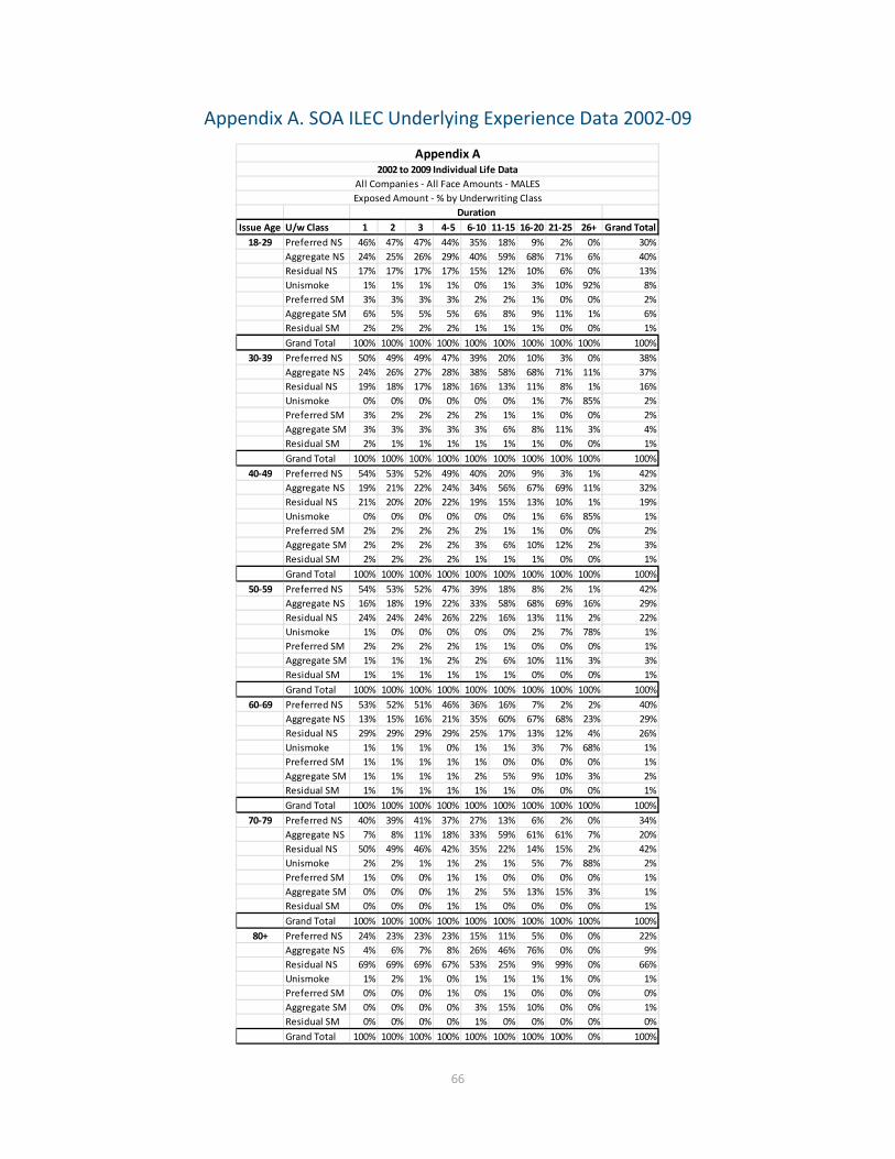
66

Appendix A. SOA ILEC Underlying Experience Data 2002-09

Issue Age U/w Class 1 2 3 4-5 6-10 11-15 16-20 21-25 26+ Grand Total18-29 Preferred NS 46% 47% 47% 44% 35% 18% 9% 2% 0% 30%

Aggregate NS 24% 25% 26% 29% 40% 59% 68% 71% 6% 40%Residual NS 17% 17% 17% 17% 15% 12% 10% 6% 0% 13%Unismoke 1% 1% 1% 1% 0% 1% 3% 10% 92% 8%Preferred SM 3% 3% 3% 3% 2% 2% 1% 0% 0% 2%Aggregate SM 6% 5% 5% 5% 6% 8% 9% 11% 1% 6%Residual SM 2% 2% 2% 2% 1% 1% 1% 0% 0% 1%Grand Total 100% 100% 100% 100% 100% 100% 100% 100% 100% 100%

30-39 Preferred NS 50% 49% 49% 47% 39% 20% 10% 3% 0% 38%Aggregate NS 24% 26% 27% 28% 38% 58% 68% 71% 11% 37%Residual NS 19% 18% 17% 18% 16% 13% 11% 8% 1% 16%Unismoke 0% 0% 0% 0% 0% 0% 1% 7% 85% 2%Preferred SM 3% 2% 2% 2% 2% 1% 1% 0% 0% 2%Aggregate SM 3% 3% 3% 3% 3% 6% 8% 11% 3% 4%Residual SM 2% 1% 1% 1% 1% 1% 1% 0% 0% 1%Grand Total 100% 100% 100% 100% 100% 100% 100% 100% 100% 100%

40-49 Preferred NS 54% 53% 52% 49% 40% 20% 9% 3% 1% 42%Aggregate NS 19% 21% 22% 24% 34% 56% 67% 69% 11% 32%Residual NS 21% 20% 20% 22% 19% 15% 13% 10% 1% 19%Unismoke 0% 0% 0% 0% 0% 0% 1% 6% 85% 1%Preferred SM 2% 2% 2% 2% 2% 1% 1% 0% 0% 2%Aggregate SM 2% 2% 2% 2% 3% 6% 10% 12% 2% 3%Residual SM 2% 2% 2% 2% 1% 1% 1% 0% 0% 1%Grand Total 100% 100% 100% 100% 100% 100% 100% 100% 100% 100%

50-59 Preferred NS 54% 53% 52% 47% 39% 18% 8% 2% 1% 42%Aggregate NS 16% 18% 19% 22% 33% 58% 68% 69% 16% 29%Residual NS 24% 24% 24% 26% 22% 16% 13% 11% 2% 22%Unismoke 1% 0% 0% 0% 0% 0% 2% 7% 78% 1%Preferred SM 2% 2% 2% 2% 1% 1% 0% 0% 0% 1%Aggregate SM 1% 1% 1% 2% 2% 6% 10% 11% 3% 3%Residual SM 1% 1% 1% 1% 1% 1% 0% 0% 0% 1%Grand Total 100% 100% 100% 100% 100% 100% 100% 100% 100% 100%

60-69 Preferred NS 53% 52% 51% 46% 36% 16% 7% 2% 2% 40%Aggregate NS 13% 15% 16% 21% 35% 60% 67% 68% 23% 29%Residual NS 29% 29% 29% 29% 25% 17% 13% 12% 4% 26%Unismoke 1% 1% 1% 0% 1% 1% 3% 7% 68% 1%Preferred SM 1% 1% 1% 1% 1% 0% 0% 0% 0% 1%Aggregate SM 1% 1% 1% 1% 2% 5% 9% 10% 3% 2%Residual SM 1% 1% 1% 1% 1% 1% 0% 0% 0% 1%Grand Total 100% 100% 100% 100% 100% 100% 100% 100% 100% 100%

70-79 Preferred NS 40% 39% 41% 37% 27% 13% 6% 2% 0% 34%Aggregate NS 7% 8% 11% 18% 33% 59% 61% 61% 7% 20%Residual NS 50% 49% 46% 42% 35% 22% 14% 15% 2% 42%Unismoke 2% 2% 1% 1% 2% 1% 5% 7% 88% 2%Preferred SM 1% 0% 0% 1% 1% 0% 0% 0% 0% 1%Aggregate SM 0% 0% 0% 1% 2% 5% 13% 15% 3% 1%Residual SM 0% 0% 0% 1% 1% 0% 0% 0% 0% 1%Grand Total 100% 100% 100% 100% 100% 100% 100% 100% 100% 100%

80+ Preferred NS 24% 23% 23% 23% 15% 11% 5% 0% 0% 22%Aggregate NS 4% 6% 7% 8% 26% 46% 76% 0% 0% 9%Residual NS 69% 69% 69% 67% 53% 25% 9% 99% 0% 66%Unismoke 1% 2% 1% 0% 1% 1% 1% 1% 0% 1%Preferred SM 0% 0% 0% 1% 0% 1% 0% 0% 0% 0%Aggregate SM 0% 0% 0% 0% 3% 15% 10% 0% 0% 1%Residual SM 0% 0% 0% 0% 1% 0% 0% 0% 0% 0%Grand Total 100% 100% 100% 100% 100% 100% 100% 100% 0% 100%

Appendix A2002 to 2009 Individual Life Data

All Companies - All Face Amounts - MALESExposed Amount - % by Underwriting Class

Duration

67

Issue Age U/w Class 1 2 3 4-5 6-10 11-15 16-20 21-25 26+ Grand Total18-29 Preferred NS 52% 53% 52% 49% 37% 19% 9% 1% 0% 35%

Aggregate NS 25% 26% 27% 31% 43% 61% 70% 72% 9% 41%Residual NS 15% 14% 14% 14% 12% 11% 9% 5% 0% 12%Unismoke 1% 1% 1% 1% 0% 1% 3% 10% 88% 4%Preferred SM 2% 2% 2% 2% 1% 1% 1% 0% 0% 1%Aggregate SM 4% 4% 4% 4% 5% 7% 9% 11% 2% 5%Residual SM 1% 1% 1% 1% 1% 1% 0% 0% 0% 1%Grand Total 100% 100% 100% 100% 100% 100% 100% 100% 100% 100%

30-39 Preferred NS 57% 56% 56% 53% 44% 21% 10% 2% 0% 44%Aggregate NS 23% 24% 26% 28% 38% 58% 69% 73% 14% 36%Residual NS 15% 14% 14% 15% 13% 12% 10% 7% 1% 13%Unismoke 0% 0% 0% 0% 0% 0% 2% 8% 82% 1%Preferred SM 2% 2% 2% 2% 1% 1% 1% 0% 0% 1%Aggregate SM 2% 2% 2% 2% 3% 7% 8% 10% 4% 4%Residual SM 1% 1% 1% 1% 1% 1% 1% 0% 0% 1%Grand Total 100% 100% 100% 100% 100% 100% 100% 100% 100% 100%

40-49 Preferred NS 57% 56% 56% 53% 45% 21% 9% 2% 0% 45%Aggregate NS 18% 19% 20% 22% 32% 54% 63% 64% 8% 30%Residual NS 19% 19% 18% 19% 17% 15% 13% 10% 1% 18%Unismoke 0% 0% 0% 0% 0% 0% 2% 10% 88% 1%Preferred SM 2% 2% 2% 2% 2% 1% 0% 0% 0% 2%Aggregate SM 2% 2% 2% 2% 3% 8% 11% 14% 2% 4%Residual SM 1% 1% 1% 1% 1% 1% 1% 0% 0% 1%Grand Total 100% 100% 100% 100% 100% 100% 100% 100% 100% 100%

50-59 Preferred NS 52% 52% 51% 48% 40% 17% 8% 2% 1% 41%Aggregate NS 16% 17% 18% 20% 30% 55% 61% 58% 9% 28%Residual NS 26% 25% 25% 26% 23% 17% 13% 11% 2% 23%Unismoke 1% 1% 0% 0% 0% 1% 3% 15% 86% 2%Preferred SM 2% 2% 2% 2% 2% 1% 0% 0% 0% 2%Aggregate SM 2% 2% 2% 2% 4% 9% 13% 13% 2% 4%Residual SM 2% 2% 2% 2% 2% 1% 1% 0% 0% 1%Grand Total 100% 100% 100% 100% 100% 100% 100% 100% 100% 100%

60-69 Preferred NS 47% 47% 46% 42% 30% 14% 8% 3% 1% 32%Aggregate NS 15% 16% 17% 21% 35% 58% 59% 59% 16% 33%Residual NS 32% 30% 30% 30% 27% 18% 14% 11% 3% 25%Unismoke 1% 1% 1% 0% 1% 1% 4% 13% 76% 2%Preferred SM 2% 2% 2% 2% 1% 0% 0% 0% 0% 1%Aggregate SM 1% 1% 2% 2% 4% 8% 13% 14% 3% 5%Residual SM 2% 2% 2% 2% 2% 1% 1% 0% 0% 2%Grand Total 100% 100% 100% 100% 100% 100% 100% 100% 100% 100%

70-79 Preferred NS 36% 36% 39% 36% 25% 13% 9% 2% 4% 30%Aggregate NS 9% 10% 12% 19% 34% 57% 60% 62% 13% 25%Residual NS 50% 48% 44% 40% 34% 21% 14% 11% 6% 39%Unismoke 2% 3% 2% 1% 2% 1% 4% 7% 72% 2%Preferred SM 1% 1% 1% 1% 1% 0% 0% 0% 0% 1%Aggregate SM 1% 1% 1% 2% 3% 6% 13% 19% 4% 3%Residual SM 1% 1% 1% 1% 1% 0% 0% 0% 0% 1%Grand Total 100% 100% 100% 100% 100% 100% 100% 100% 100% 100%

80+ Preferred NS 24% 24% 23% 23% 18% 8% 11% 0% 0% 22%Aggregate NS 6% 7% 8% 12% 26% 60% 45% 87% 0% 13%Residual NS 68% 67% 66% 62% 51% 25% 6% 12% 0% 62%Unismoke 1% 1% 1% 1% 2% 2% 1% 0% 0% 1%Preferred SM 0% 0% 0% 0% 0% 0% 0% 0% 0% 0%Aggregate SM 1% 1% 1% 1% 2% 6% 37% 0% 0% 1%Residual SM 0% 0% 1% 1% 1% 0% 0% 0% 0% 1%Grand Total 100% 100% 100% 100% 100% 100% 100% 100% 0% 100%

Appendix A2002 to 2009 Individual Life Data

All Companies - All Face Amounts - FEMALESExposed Amount - % by Underwriting Class

Duration

68

Appendix B. Adjustments of Experience to Current Business Distribution

Assuming current Preferred/Non-Preferred business distribution existed through the whole study.

Dur/Age 25 35 45 55 65 75 85

1 100.0% 100.0% 100.0% 100.0% 100.0% 100.0% 100.0% 2 100.0% 100.0% 100.0% 100.0% 100.0% 100.0% 100.0% 3 100.0% 100.0% 100.0% 100.0% 99.9% 100.0% 100.0% 4 100.0% 100.0% 100.0% 100.0% 99.8% 100.0% 100.0% 5 100.0% 100.0% 100.0% 100.0% 99.7% 100.0% 100.0% 6 100.0% 100.0% 100.0% 100.0% 99.5% 100.0% 100.0% 7 100.0% 100.0% 99.9% 99.9% 99.4% 100.0% 100.0% 8 99.8% 99.8% 99.7% 99.6% 99.2% 100.0% 100.0% 9 99.4% 99.4% 99.4% 99.4% 99.1% 100.0% 100.0%

10 99.1% 99.1% 99.1% 99.2% 99.0% 100.0% 100.0% 11 98.7% 98.7% 98.8% 98.9% 98.8% 100.0% 100.0% 12 98.3% 98.3% 98.5% 98.7% 98.7% 100.0% 100.0% 13 98.0% 98.0% 98.2% 98.5% 98.5% 100.0% 100.0% 14 97.6% 97.6% 97.9% 98.3% 98.4% 99.9% 100.0% 15 97.2% 97.2% 97.6% 98.0% 98.3% 99.8% 100.0% 16 96.8% 96.8% 97.3% 97.8% 98.1% 99.8% 100.0% 17 96.5% 96.5% 97.0% 97.6% 98.0% 99.7% 100.0% 18 96.1% 96.1% 96.7% 97.3% 97.8% 99.7% 100.0% 19 95.7% 95.7% 96.4% 97.1% 97.7% 99.6% 100.0% 20 95.4% 95.4% 96.1% 96.9% 97.6% 99.6% 100.0% 21 95.0% 95.0% 95.8% 96.6% 97.4% 99.5% 100.0% 22 94.6% 94.6% 95.5% 96.4% 97.3% 99.4% 100.0% 23 94.3% 94.3% 95.2% 96.2% 97.1% 99.4% 100.0% 24 93.9% 93.9% 94.9% 95.9% 97.0% 99.3% 100.0% 25 93.5% 93.5% 94.6% 95.7% 96.9% 99.3% 100.0%

69

Appendix C. Development of Age Last Birthday (ALB) Tables

The following algorithm was used to convert the ANB mortality rates to ALB rates.

1. Naming convention:

a. Template: 2015 VBT (Sex) Smoking Type Basis

b. Sex:

M. Male

F. Female

c. Smoking:

NS. Non-smoker

SM. Smoker

d. Type:

S&U. Select & ultimate

U. Ultimate

e. Basis:

ANB. Age nearest birthday

ALB. Age last birthday

Example: 2015 VBT (M) NS U ALB is the male non-smoker table based on the ultimate portion of the table and is age last birthday for the primary underwriting tables. 2015 VBT (F) NS S&U ANB is the select and ultimate portion of the female non-smoker primary underwriting table and is age nearest birthday.

Groups of tables. When an item is not identified, all versions of that item are included. For example, 2008 VBT (M) S&U would include all of the select & ultimate tables for males, including non-smoker, smoker, age nearest birthday and age last birthday.

2. Starting basis

The starting point for building the age last birthday tables was the respective age nearest birthday table.

70

3. Select & Ultimate tables

Values for these tables are calculated according to the following methodology.

• The mortality rates per 1,000 lives are rounded to two decimal places. Select period values for all issue ages are developed from age nearest birthday rates that are in the same duration. For issue age 95, approximate issue age 96 ANB rates for duration 1 were created by assuming constant 3rd differences from the issue ages 92-95. Duration 2+ rates are on an ultimate period basis.

• Composite rates for young ages. All rates for attained ages 17 and younger are on a composite smoking basis. Smoker and non-smoker rates are the same. Rates for issue ages 10-17, durations 1-7 and attained age under 17 are set on a select and ultimate basis. The others are set at the ultimate rate calculated from issue age 0 rates.

• The calculation of the attained age 17 select and ultimate ALB rates used a composite issue age 18 ANB rate. This age 18 ANB rate was extrapolated from attained ages 15-17 by assuming a constant 2nd difference at each duration. This ensured that the attained age 17 rates remained on a composite basis.

• Age 0 ALB rates were set at 87.67% and 84.37% of age 0 ANB rates for females and males, respectively. This was based on an analysis of 2003 population age 0 rates. It was assumed that insurance coverage begins after 15 days and that 50% of issues would occur at age 15 days. The other 50% of issues occurred evenly throughout the remainder of the first year.

4. Ultimate tables

Separate ultimate versions of the tables were not developed, but can be extracted from the ultimate column of the respective select and ultimate tables.

71

Appendix D. Sample RR Mortality Rate Calculations

Below are two example calculations showing how RR mortality rates were developed. Please note that these calculations were originally performed on unrounded numbers. If the rounded, published numbers are used as inputs to replicate the calculations, in some cases the result will be slightly different than those in the published 2015 RR tables when rounded to two decimal places.

Example #1: Calculating the 2015 RR 80 rate for a male non-smoker at issue age 45, duration 1.

(1) 𝑞𝑞[𝑥𝑥]15 𝑅𝑅𝑅𝑅 80 = 𝑞𝑞[𝑥𝑥]

15 𝑅𝑅𝑅𝑅 100 ∙𝑞𝑞[𝑥𝑥]08 𝑅𝑅𝑅𝑅 80

𝑞𝑞[𝑥𝑥]08 𝑅𝑅𝑅𝑅 100

𝑞𝑞[45]15 𝑅𝑅𝑅𝑅 100 = 0.55 [Source – 2015 Relative Risk tables, published simultaneously with this report]

𝑞𝑞[45]08 𝑅𝑅𝑅𝑅 80 = 0.63 [Source – 2008 Relative Risk tables, published with 2008 VBT report]

𝑞𝑞[45]08 𝑅𝑅𝑅𝑅 100 = 0.83 [Source – 2008 Relative Risk tables, published with 2008 VBT report]

𝑞𝑞[45]15 𝑅𝑅𝑅𝑅 80 = 0.55 ∙ 0.63

0.83 = 0.42

Example #2: Calculating the 2015 RR 50 rate for a male non-smoker at issue age 55, duration 1. (Similar sources as for Example #1 were used.)

(5) 𝑞𝑞[𝑥𝑥]15 𝑅𝑅𝑅𝑅 50 = 𝑞𝑞[𝑥𝑥]

15 𝑅𝑅𝑅𝑅 100 ∙ �1 −�𝑞𝑞[𝑥𝑥]

08 𝑅𝑅𝑅𝑅 100−𝑞𝑞[𝑥𝑥]08 𝑅𝑅𝑅𝑅 70�∙(100−50)

(100−70)

𝑞𝑞[𝑥𝑥]08 𝑅𝑅𝑅𝑅 100 �

𝑞𝑞[55]15 𝑅𝑅𝑅𝑅 100 = 0.55

𝑞𝑞[55]08 𝑅𝑅𝑅𝑅 100 = 0.83

𝑞𝑞[55]08 𝑅𝑅𝑅𝑅 70 = 0.54

𝑞𝑞[55]15 𝑅𝑅𝑅𝑅 50 = 0.55 ∙ �1 −

(0.83−0.54)∙(100−50)(100−70)

0.83� = 0.23

72

Appendix E. Monotonicity Adjustments

Issue #1: For a given duration, the rate at a given issue age is lower than the rate at the issue age preceding it

Generally, this was fixed by setting the rate (x, y) at issue age x and duration y equal to either the rate at (x+1, y) or (x-1, y), depending on which method resulted in the fewest adjustments.

o Because affected cells were often adjacent to one another within a column, it was often possible to minimize the number of adjustments by varying whether to set the (x, y) rate equal to the rate at (x+1, y) or (x-1, y)

Below attained age 30, no monotonicity adjustments were made for this issue, as mortality experience did not necessarily increase with age.

Issue #2: For a given issue age, the rate at a given duration is lower than the rate at the duration preceding it

No monotonicity errors were discovered for this issue, so no adjustments were needed.

Issue #3: For a given attained age, the rate at a given duration is lower than the rate at the duration preceding it

No monotonicity errors were discovered for this issue, so no adjustments were needed.

Issue #4: Female rates are higher than corresponding male rates

• To correct this, the female rate was recalculated as the corresponding male rate multiplied by the ratio of the female rate to the male rate for either the issue age above or below the affected region (depending on which ratio is closest to 100%) at the same duration.

• Example: o Let FSMx,y be the mortality rate for female smokers at age x and duration y o Let MSMx,y be the mortality rate for male smokers at age x and duration y o Suppose FSMx,3 > MSMx,3 for all x from 76-89

First, we compare the ratios (FSM75,3 / MSM75,3) and (FSM90,3 / MSM90,3) Whichever ratio is higher (closer to 100%) is selected as the ratio to apply to the

corresponding male rates for the affected region in the female table. Suppose for this example that the age-75 ratio, (FSM75,3 / MSM75,3) is higher

Then, for all x from 76-89, FSMx,3 = MSMx,3 * (FSM75,3 / MSM75,3) • Note that in some cases, this fix resulted in some monotonicity issues along a diagonal.

o For example, for female smokers, after applying the above fix, for some (x,y), FSMx,y > FSMx-

1,y+1 o This issue was fixed by interpolating between the rates for unaffected cells along the

diagonal. For example, if just one consecutive cell FSMx,y on a diagonal had the monotonicity

issue, then FSMx,y = (FSMx+1,y-1 + FSMx-1,y+1) / 2

Issue #5: Smoker rates are lower than corresponding non-smoker rates

To correct this, smoker rates were set equal to the corresponding non-smoker rates.

73

Appendix F. Preferred Wear-off Factors

1 2 3 4 5 6 7 8 9 10 11 12 130 0.0% 0.0% 0.0% 0.0% 0.0% 0.0% 0.0% 0.0% 0.0% 0.0% 0.0% 0.0% 0.0%1 0.0% 0.0% 0.0% 0.0% 0.0% 0.0% 0.0% 0.0% 0.0% 0.0% 0.0% 0.0% 0.0%2 0.0% 0.0% 0.0% 0.0% 0.0% 0.0% 0.0% 0.0% 0.0% 0.0% 0.0% 0.0% 0.0%3 0.0% 0.0% 0.0% 0.0% 0.0% 0.0% 0.0% 0.0% 0.0% 0.0% 0.0% 0.0% 0.0%4 0.0% 0.0% 0.0% 0.0% 0.0% 0.0% 0.0% 0.0% 0.0% 0.0% 0.0% 0.0% 0.0%5 0.0% 0.0% 0.0% 0.0% 0.0% 0.0% 0.0% 0.0% 0.0% 0.0% 0.0% 0.0% 0.0%6 0.0% 0.0% 0.0% 0.0% 0.0% 0.0% 0.0% 0.0% 0.0% 0.0% 0.0% 0.0% 0.0%7 0.0% 0.0% 0.0% 0.0% 0.0% 0.0% 0.0% 0.0% 0.0% 0.0% 0.0% 0.0% 0.0%8 0.0% 0.0% 0.0% 0.0% 0.0% 0.0% 0.0% 0.0% 0.0% 0.0% 0.0% 0.0% 0.0%9 0.0% 0.0% 0.0% 0.0% 0.0% 0.0% 0.0% 0.0% 0.0% 0.0% 0.0% 0.0% 0.0%

10 0.0% 0.0% 0.0% 0.0% 0.0% 0.0% 0.0% 0.0% 0.0% 0.0% 0.0% 0.0% 0.0%11 0.0% 0.0% 0.0% 0.0% 0.0% 0.0% 0.0% 0.0% 0.0% 0.0% 0.0% 0.0% 0.0%12 0.0% 0.0% 0.0% 0.0% 0.0% 0.0% 0.0% 0.0% 0.0% 0.0% 0.0% 0.0% 0.0%13 0.0% 0.0% 0.0% 0.0% 0.0% 0.0% 0.0% 0.0% 0.0% 0.0% 0.0% 0.0% 0.0%14 0.0% 0.0% 0.0% 0.0% 0.0% 0.0% 0.0% 0.0% 0.0% 0.0% 0.0% 0.0% 0.0%15 0.0% 0.0% 0.0% 0.0% 0.0% 0.0% 0.0% 0.0% 0.0% 0.0% 0.0% 0.0% 0.0%16 0.0% 0.0% 0.0% 0.0% 0.0% 0.0% 0.0% 0.0% 0.0% 0.0% 0.0% 0.0% 0.0%17 0.0% 0.0% 0.0% 0.0% 0.0% 0.0% 0.0% 0.0% 0.0% 0.0% 0.0% 0.0% 0.0%18 0.0% 0.0% 0.0% 0.0% 0.0% 0.0% 0.0% 0.0% 0.0% 0.0% 0.0% 0.0% 0.0%19 0.0% 0.0% 0.0% 0.0% 0.0% 0.0% 0.0% 0.0% 0.0% 0.0% 0.0% 0.0% 0.0%20 0.0% 0.0% 0.0% 0.0% 0.0% 0.0% 0.0% 0.0% 0.0% 0.0% 0.0% 0.0% 0.0%21 0.0% 0.0% 0.0% 0.0% 0.0% 0.0% 0.0% 0.0% 0.0% 0.0% 0.0% 0.0% 0.0%22 0.0% 0.0% 0.0% 0.0% 0.0% 0.0% 0.0% 0.0% 0.0% 0.0% 0.0% 0.0% 0.0%23 0.0% 0.0% 0.0% 0.0% 0.0% 0.0% 0.0% 0.0% 0.0% 0.0% 0.0% 0.0% 0.0%24 0.0% 0.0% 0.0% 0.0% 0.0% 0.0% 0.0% 0.0% 0.0% 0.0% 0.0% 0.0% 0.0%25 0.0% 0.0% 0.0% 0.0% 0.0% 0.0% 0.0% 0.0% 0.0% 0.0% 0.0% 0.0% 0.0%26 0.0% 0.0% 0.0% 0.0% 0.0% 0.0% 0.0% 0.0% 0.0% 0.0% 0.0% 0.0% 0.0%27 0.0% 0.0% 0.0% 0.0% 0.0% 0.0% 0.0% 0.0% 0.0% 0.0% 0.0% 0.0% 0.0%28 0.0% 0.0% 0.0% 0.0% 0.0% 0.0% 0.0% 0.0% 0.0% 0.0% 0.0% 0.0% 0.0%29 0.0% 0.0% 0.0% 0.0% 0.0% 0.0% 0.0% 0.0% 0.0% 0.0% 0.0% 0.0% 0.0%30 0.0% 0.0% 0.0% 0.0% 0.0% 0.0% 0.0% 0.0% 0.0% 0.0% 0.0% 0.0% 0.0%31 0.0% 0.0% 0.0% 0.0% 0.0% 0.0% 0.0% 0.0% 0.0% 0.0% 0.0% 0.0% 0.0%32 0.0% 0.0% 0.0% 0.0% 0.0% 0.0% 0.0% 0.0% 0.0% 0.0% 0.0% 0.0% 0.0%33 0.0% 0.0% 0.0% 0.0% 0.0% 0.0% 0.0% 0.0% 0.0% 0.0% 0.0% 0.0% 0.0%34 0.0% 0.0% 0.0% 0.0% 0.0% 0.0% 0.0% 0.0% 0.0% 0.0% 0.0% 0.0% 0.5%35 0.0% 0.0% 0.0% 0.0% 0.0% 0.0% 0.0% 0.0% 0.0% 0.0% 0.0% 0.5% 1.1%36 0.0% 0.0% 0.0% 0.0% 0.0% 0.0% 0.0% 0.0% 0.0% 0.0% 0.5% 1.0% 1.6%37 0.0% 0.0% 0.0% 0.0% 0.0% 0.0% 0.0% 0.0% 0.0% 0.5% 1.0% 1.6% 2.1%38 0.0% 0.0% 0.0% 0.0% 0.0% 0.0% 0.0% 0.0% 0.5% 1.0% 1.6% 2.1% 2.6%39 0.0% 0.0% 0.0% 0.0% 0.0% 0.0% 0.0% 0.5% 1.0% 1.5% 2.1% 2.6% 3.2%40 0.0% 0.0% 0.0% 0.0% 0.0% 0.0% 0.5% 1.0% 1.5% 2.1% 2.6% 3.2% 3.9%41 0.0% 0.0% 0.0% 0.0% 0.0% 0.5% 1.0% 1.5% 2.0% 2.6% 3.2% 3.8% 4.6%42 0.0% 0.0% 0.0% 0.0% 0.0% 0.9% 1.4% 2.0% 2.5% 3.1% 3.8% 4.6% 5.5%43 0.0% 0.0% 0.0% 0.0% 0.9% 1.4% 1.9% 2.5% 3.1% 3.8% 4.5% 5.4% 6.4%44 0.0% 0.0% 0.0% 0.8% 1.3% 1.9% 2.4% 3.0% 3.7% 4.5% 5.4% 6.3% 7.4%45 0.0% 0.0% 0.7% 1.3% 1.8% 2.3% 2.9% 3.6% 4.4% 5.3% 6.3% 7.4% 8.5%46 0.0% 0.6% 1.1% 1.7% 2.2% 2.8% 3.5% 4.3% 5.2% 6.2% 7.3% 8.5% 9.7%47 0.0% 0.6% 1.1% 1.7% 2.3% 3.0% 3.8% 4.7% 5.7% 6.8% 7.9% 9.2% 10.6%48 0.0% 0.6% 1.1% 1.7% 2.5% 3.3% 4.2% 5.1% 6.2% 7.4% 8.7% 10.1% 11.5%49 0.0% 0.6% 1.2% 1.9% 2.7% 3.6% 4.6% 5.7% 6.9% 8.2% 9.6% 11.0% 12.6%

DurationIssue Age

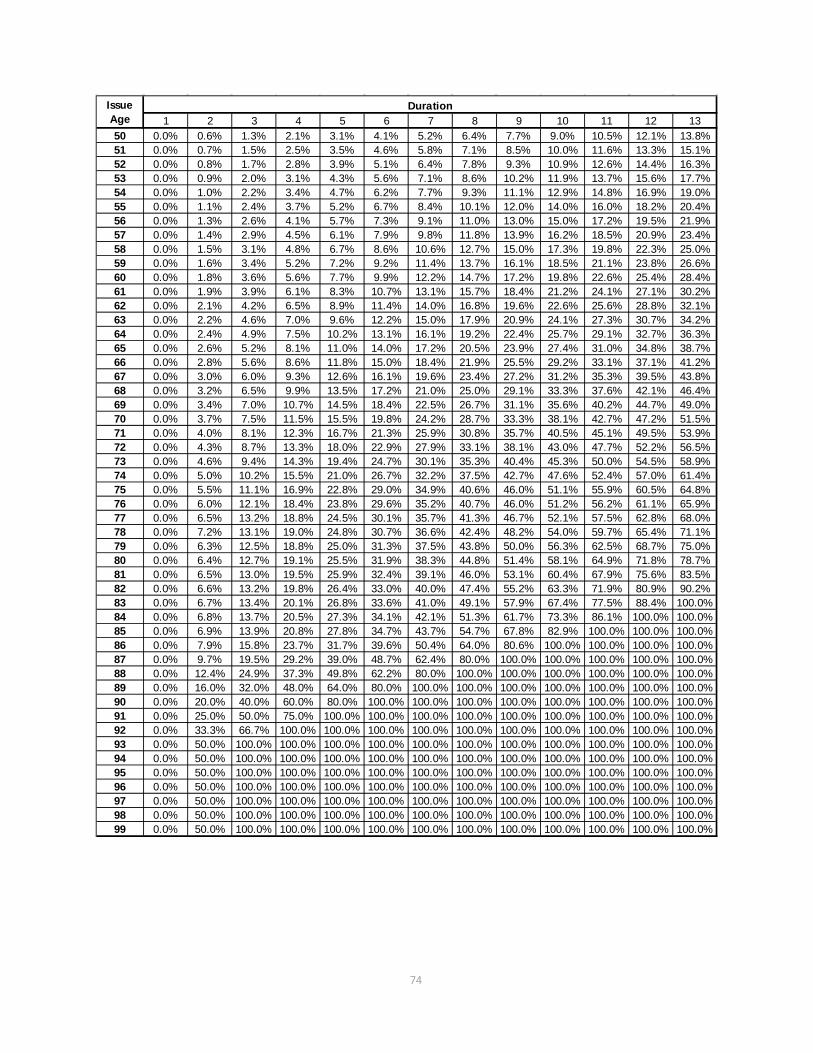
74

1 2 3 4 5 6 7 8 9 10 11 12 1350 0.0% 0.6% 1.3% 2.1% 3.1% 4.1% 5.2% 6.4% 7.7% 9.0% 10.5% 12.1% 13.8%51 0.0% 0.7% 1.5% 2.5% 3.5% 4.6% 5.8% 7.1% 8.5% 10.0% 11.6% 13.3% 15.1%52 0.0% 0.8% 1.7% 2.8% 3.9% 5.1% 6.4% 7.8% 9.3% 10.9% 12.6% 14.4% 16.3%53 0.0% 0.9% 2.0% 3.1% 4.3% 5.6% 7.1% 8.6% 10.2% 11.9% 13.7% 15.6% 17.7%54 0.0% 1.0% 2.2% 3.4% 4.7% 6.2% 7.7% 9.3% 11.1% 12.9% 14.8% 16.9% 19.0%55 0.0% 1.1% 2.4% 3.7% 5.2% 6.7% 8.4% 10.1% 12.0% 14.0% 16.0% 18.2% 20.4%56 0.0% 1.3% 2.6% 4.1% 5.7% 7.3% 9.1% 11.0% 13.0% 15.0% 17.2% 19.5% 21.9%57 0.0% 1.4% 2.9% 4.5% 6.1% 7.9% 9.8% 11.8% 13.9% 16.2% 18.5% 20.9% 23.4%58 0.0% 1.5% 3.1% 4.8% 6.7% 8.6% 10.6% 12.7% 15.0% 17.3% 19.8% 22.3% 25.0%59 0.0% 1.6% 3.4% 5.2% 7.2% 9.2% 11.4% 13.7% 16.1% 18.5% 21.1% 23.8% 26.6%60 0.0% 1.8% 3.6% 5.6% 7.7% 9.9% 12.2% 14.7% 17.2% 19.8% 22.6% 25.4% 28.4%61 0.0% 1.9% 3.9% 6.1% 8.3% 10.7% 13.1% 15.7% 18.4% 21.2% 24.1% 27.1% 30.2%62 0.0% 2.1% 4.2% 6.5% 8.9% 11.4% 14.0% 16.8% 19.6% 22.6% 25.6% 28.8% 32.1%63 0.0% 2.2% 4.6% 7.0% 9.6% 12.2% 15.0% 17.9% 20.9% 24.1% 27.3% 30.7% 34.2%64 0.0% 2.4% 4.9% 7.5% 10.2% 13.1% 16.1% 19.2% 22.4% 25.7% 29.1% 32.7% 36.3%65 0.0% 2.6% 5.2% 8.1% 11.0% 14.0% 17.2% 20.5% 23.9% 27.4% 31.0% 34.8% 38.7%66 0.0% 2.8% 5.6% 8.6% 11.8% 15.0% 18.4% 21.9% 25.5% 29.2% 33.1% 37.1% 41.2%67 0.0% 3.0% 6.0% 9.3% 12.6% 16.1% 19.6% 23.4% 27.2% 31.2% 35.3% 39.5% 43.8%68 0.0% 3.2% 6.5% 9.9% 13.5% 17.2% 21.0% 25.0% 29.1% 33.3% 37.6% 42.1% 46.4%69 0.0% 3.4% 7.0% 10.7% 14.5% 18.4% 22.5% 26.7% 31.1% 35.6% 40.2% 44.7% 49.0%70 0.0% 3.7% 7.5% 11.5% 15.5% 19.8% 24.2% 28.7% 33.3% 38.1% 42.7% 47.2% 51.5%71 0.0% 4.0% 8.1% 12.3% 16.7% 21.3% 25.9% 30.8% 35.7% 40.5% 45.1% 49.5% 53.9%72 0.0% 4.3% 8.7% 13.3% 18.0% 22.9% 27.9% 33.1% 38.1% 43.0% 47.7% 52.2% 56.5%73 0.0% 4.6% 9.4% 14.3% 19.4% 24.7% 30.1% 35.3% 40.4% 45.3% 50.0% 54.5% 58.9%74 0.0% 5.0% 10.2% 15.5% 21.0% 26.7% 32.2% 37.5% 42.7% 47.6% 52.4% 57.0% 61.4%75 0.0% 5.5% 11.1% 16.9% 22.8% 29.0% 34.9% 40.6% 46.0% 51.1% 55.9% 60.5% 64.8%76 0.0% 6.0% 12.1% 18.4% 23.8% 29.6% 35.2% 40.7% 46.0% 51.2% 56.2% 61.1% 65.9%77 0.0% 6.5% 13.2% 18.8% 24.5% 30.1% 35.7% 41.3% 46.7% 52.1% 57.5% 62.8% 68.0%78 0.0% 7.2% 13.1% 19.0% 24.8% 30.7% 36.6% 42.4% 48.2% 54.0% 59.7% 65.4% 71.1%79 0.0% 6.3% 12.5% 18.8% 25.0% 31.3% 37.5% 43.8% 50.0% 56.3% 62.5% 68.7% 75.0%80 0.0% 6.4% 12.7% 19.1% 25.5% 31.9% 38.3% 44.8% 51.4% 58.1% 64.9% 71.8% 78.7%81 0.0% 6.5% 13.0% 19.5% 25.9% 32.4% 39.1% 46.0% 53.1% 60.4% 67.9% 75.6% 83.5%82 0.0% 6.6% 13.2% 19.8% 26.4% 33.0% 40.0% 47.4% 55.2% 63.3% 71.9% 80.9% 90.2%83 0.0% 6.7% 13.4% 20.1% 26.8% 33.6% 41.0% 49.1% 57.9% 67.4% 77.5% 88.4% 100.0%84 0.0% 6.8% 13.7% 20.5% 27.3% 34.1% 42.1% 51.3% 61.7% 73.3% 86.1% 100.0% 100.0%85 0.0% 6.9% 13.9% 20.8% 27.8% 34.7% 43.7% 54.7% 67.8% 82.9% 100.0% 100.0% 100.0%86 0.0% 7.9% 15.8% 23.7% 31.7% 39.6% 50.4% 64.0% 80.6% 100.0% 100.0% 100.0% 100.0%87 0.0% 9.7% 19.5% 29.2% 39.0% 48.7% 62.4% 80.0% 100.0% 100.0% 100.0% 100.0% 100.0%88 0.0% 12.4% 24.9% 37.3% 49.8% 62.2% 80.0% 100.0% 100.0% 100.0% 100.0% 100.0% 100.0%89 0.0% 16.0% 32.0% 48.0% 64.0% 80.0% 100.0% 100.0% 100.0% 100.0% 100.0% 100.0% 100.0%90 0.0% 20.0% 40.0% 60.0% 80.0% 100.0% 100.0% 100.0% 100.0% 100.0% 100.0% 100.0% 100.0%91 0.0% 25.0% 50.0% 75.0% 100.0% 100.0% 100.0% 100.0% 100.0% 100.0% 100.0% 100.0% 100.0%92 0.0% 33.3% 66.7% 100.0% 100.0% 100.0% 100.0% 100.0% 100.0% 100.0% 100.0% 100.0% 100.0%93 0.0% 50.0% 100.0% 100.0% 100.0% 100.0% 100.0% 100.0% 100.0% 100.0% 100.0% 100.0% 100.0%94 0.0% 50.0% 100.0% 100.0% 100.0% 100.0% 100.0% 100.0% 100.0% 100.0% 100.0% 100.0% 100.0%95 0.0% 50.0% 100.0% 100.0% 100.0% 100.0% 100.0% 100.0% 100.0% 100.0% 100.0% 100.0% 100.0%96 0.0% 50.0% 100.0% 100.0% 100.0% 100.0% 100.0% 100.0% 100.0% 100.0% 100.0% 100.0% 100.0%97 0.0% 50.0% 100.0% 100.0% 100.0% 100.0% 100.0% 100.0% 100.0% 100.0% 100.0% 100.0% 100.0%98 0.0% 50.0% 100.0% 100.0% 100.0% 100.0% 100.0% 100.0% 100.0% 100.0% 100.0% 100.0% 100.0%99 0.0% 50.0% 100.0% 100.0% 100.0% 100.0% 100.0% 100.0% 100.0% 100.0% 100.0% 100.0% 100.0%

DurationIssue Age

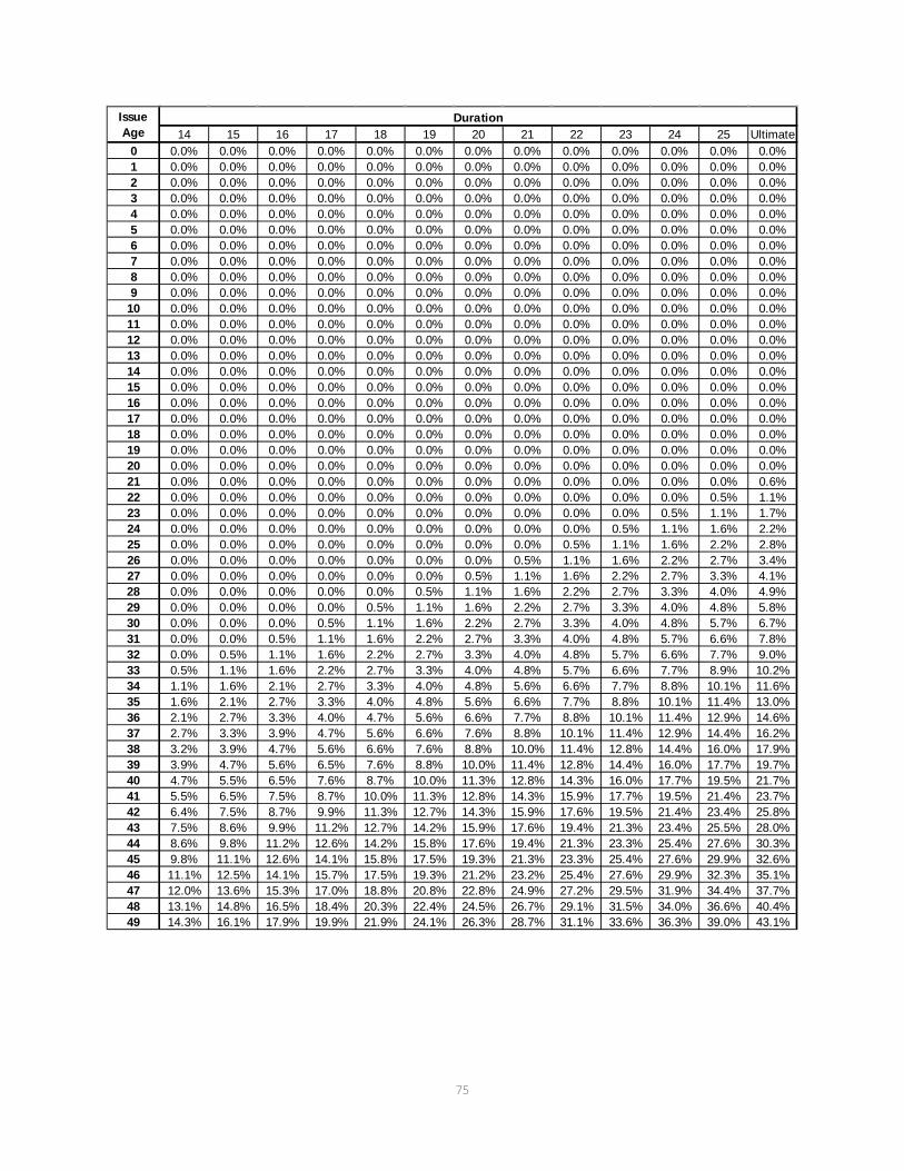
75

14 15 16 17 18 19 20 21 22 23 24 25 Ultimate0 0.0% 0.0% 0.0% 0.0% 0.0% 0.0% 0.0% 0.0% 0.0% 0.0% 0.0% 0.0% 0.0%1 0.0% 0.0% 0.0% 0.0% 0.0% 0.0% 0.0% 0.0% 0.0% 0.0% 0.0% 0.0% 0.0%2 0.0% 0.0% 0.0% 0.0% 0.0% 0.0% 0.0% 0.0% 0.0% 0.0% 0.0% 0.0% 0.0%3 0.0% 0.0% 0.0% 0.0% 0.0% 0.0% 0.0% 0.0% 0.0% 0.0% 0.0% 0.0% 0.0%4 0.0% 0.0% 0.0% 0.0% 0.0% 0.0% 0.0% 0.0% 0.0% 0.0% 0.0% 0.0% 0.0%5 0.0% 0.0% 0.0% 0.0% 0.0% 0.0% 0.0% 0.0% 0.0% 0.0% 0.0% 0.0% 0.0%6 0.0% 0.0% 0.0% 0.0% 0.0% 0.0% 0.0% 0.0% 0.0% 0.0% 0.0% 0.0% 0.0%7 0.0% 0.0% 0.0% 0.0% 0.0% 0.0% 0.0% 0.0% 0.0% 0.0% 0.0% 0.0% 0.0%8 0.0% 0.0% 0.0% 0.0% 0.0% 0.0% 0.0% 0.0% 0.0% 0.0% 0.0% 0.0% 0.0%9 0.0% 0.0% 0.0% 0.0% 0.0% 0.0% 0.0% 0.0% 0.0% 0.0% 0.0% 0.0% 0.0%

10 0.0% 0.0% 0.0% 0.0% 0.0% 0.0% 0.0% 0.0% 0.0% 0.0% 0.0% 0.0% 0.0%11 0.0% 0.0% 0.0% 0.0% 0.0% 0.0% 0.0% 0.0% 0.0% 0.0% 0.0% 0.0% 0.0%12 0.0% 0.0% 0.0% 0.0% 0.0% 0.0% 0.0% 0.0% 0.0% 0.0% 0.0% 0.0% 0.0%13 0.0% 0.0% 0.0% 0.0% 0.0% 0.0% 0.0% 0.0% 0.0% 0.0% 0.0% 0.0% 0.0%14 0.0% 0.0% 0.0% 0.0% 0.0% 0.0% 0.0% 0.0% 0.0% 0.0% 0.0% 0.0% 0.0%15 0.0% 0.0% 0.0% 0.0% 0.0% 0.0% 0.0% 0.0% 0.0% 0.0% 0.0% 0.0% 0.0%16 0.0% 0.0% 0.0% 0.0% 0.0% 0.0% 0.0% 0.0% 0.0% 0.0% 0.0% 0.0% 0.0%17 0.0% 0.0% 0.0% 0.0% 0.0% 0.0% 0.0% 0.0% 0.0% 0.0% 0.0% 0.0% 0.0%18 0.0% 0.0% 0.0% 0.0% 0.0% 0.0% 0.0% 0.0% 0.0% 0.0% 0.0% 0.0% 0.0%19 0.0% 0.0% 0.0% 0.0% 0.0% 0.0% 0.0% 0.0% 0.0% 0.0% 0.0% 0.0% 0.0%20 0.0% 0.0% 0.0% 0.0% 0.0% 0.0% 0.0% 0.0% 0.0% 0.0% 0.0% 0.0% 0.0%21 0.0% 0.0% 0.0% 0.0% 0.0% 0.0% 0.0% 0.0% 0.0% 0.0% 0.0% 0.0% 0.6%22 0.0% 0.0% 0.0% 0.0% 0.0% 0.0% 0.0% 0.0% 0.0% 0.0% 0.0% 0.5% 1.1%23 0.0% 0.0% 0.0% 0.0% 0.0% 0.0% 0.0% 0.0% 0.0% 0.0% 0.5% 1.1% 1.7%24 0.0% 0.0% 0.0% 0.0% 0.0% 0.0% 0.0% 0.0% 0.0% 0.5% 1.1% 1.6% 2.2%25 0.0% 0.0% 0.0% 0.0% 0.0% 0.0% 0.0% 0.0% 0.5% 1.1% 1.6% 2.2% 2.8%26 0.0% 0.0% 0.0% 0.0% 0.0% 0.0% 0.0% 0.5% 1.1% 1.6% 2.2% 2.7% 3.4%27 0.0% 0.0% 0.0% 0.0% 0.0% 0.0% 0.5% 1.1% 1.6% 2.2% 2.7% 3.3% 4.1%28 0.0% 0.0% 0.0% 0.0% 0.0% 0.5% 1.1% 1.6% 2.2% 2.7% 3.3% 4.0% 4.9%29 0.0% 0.0% 0.0% 0.0% 0.5% 1.1% 1.6% 2.2% 2.7% 3.3% 4.0% 4.8% 5.8%30 0.0% 0.0% 0.0% 0.5% 1.1% 1.6% 2.2% 2.7% 3.3% 4.0% 4.8% 5.7% 6.7%31 0.0% 0.0% 0.5% 1.1% 1.6% 2.2% 2.7% 3.3% 4.0% 4.8% 5.7% 6.6% 7.8%32 0.0% 0.5% 1.1% 1.6% 2.2% 2.7% 3.3% 4.0% 4.8% 5.7% 6.6% 7.7% 9.0%33 0.5% 1.1% 1.6% 2.2% 2.7% 3.3% 4.0% 4.8% 5.7% 6.6% 7.7% 8.9% 10.2%34 1.1% 1.6% 2.1% 2.7% 3.3% 4.0% 4.8% 5.6% 6.6% 7.7% 8.8% 10.1% 11.6%35 1.6% 2.1% 2.7% 3.3% 4.0% 4.8% 5.6% 6.6% 7.7% 8.8% 10.1% 11.4% 13.0%36 2.1% 2.7% 3.3% 4.0% 4.7% 5.6% 6.6% 7.7% 8.8% 10.1% 11.4% 12.9% 14.6%37 2.7% 3.3% 3.9% 4.7% 5.6% 6.6% 7.6% 8.8% 10.1% 11.4% 12.9% 14.4% 16.2%38 3.2% 3.9% 4.7% 5.6% 6.6% 7.6% 8.8% 10.0% 11.4% 12.8% 14.4% 16.0% 17.9%39 3.9% 4.7% 5.6% 6.5% 7.6% 8.8% 10.0% 11.4% 12.8% 14.4% 16.0% 17.7% 19.7%40 4.7% 5.5% 6.5% 7.6% 8.7% 10.0% 11.3% 12.8% 14.3% 16.0% 17.7% 19.5% 21.7%41 5.5% 6.5% 7.5% 8.7% 10.0% 11.3% 12.8% 14.3% 15.9% 17.7% 19.5% 21.4% 23.7%42 6.4% 7.5% 8.7% 9.9% 11.3% 12.7% 14.3% 15.9% 17.6% 19.5% 21.4% 23.4% 25.8%43 7.5% 8.6% 9.9% 11.2% 12.7% 14.2% 15.9% 17.6% 19.4% 21.3% 23.4% 25.5% 28.0%44 8.6% 9.8% 11.2% 12.6% 14.2% 15.8% 17.6% 19.4% 21.3% 23.3% 25.4% 27.6% 30.3%45 9.8% 11.1% 12.6% 14.1% 15.8% 17.5% 19.3% 21.3% 23.3% 25.4% 27.6% 29.9% 32.6%46 11.1% 12.5% 14.1% 15.7% 17.5% 19.3% 21.2% 23.2% 25.4% 27.6% 29.9% 32.3% 35.1%47 12.0% 13.6% 15.3% 17.0% 18.8% 20.8% 22.8% 24.9% 27.2% 29.5% 31.9% 34.4% 37.7%48 13.1% 14.8% 16.5% 18.4% 20.3% 22.4% 24.5% 26.7% 29.1% 31.5% 34.0% 36.6% 40.4%49 14.3% 16.1% 17.9% 19.9% 21.9% 24.1% 26.3% 28.7% 31.1% 33.6% 36.3% 39.0% 43.1%

DurationIssue Age

76

14 15 16 17 18 19 20 21 22 23 24 25 Ultimate50 15.6% 17.5% 19.4% 21.5% 23.6% 25.9% 28.3% 30.7% 33.3% 35.9% 38.6% 41.5% 46.0%51 16.9% 18.9% 21.0% 23.2% 25.4% 27.8% 30.3% 32.8% 35.5% 38.3% 41.1% 44.1% 48.9%52 18.3% 20.4% 22.6% 24.9% 27.3% 29.8% 32.4% 35.0% 37.8% 40.7% 43.7% 46.7% 51.9%53 19.8% 22.0% 24.3% 26.7% 29.2% 31.8% 34.5% 37.3% 40.2% 43.2% 46.3% 49.5% 55.1%54 21.2% 23.6% 26.0% 28.5% 31.2% 33.9% 36.7% 39.6% 42.7% 45.8% 49.0% 52.3% 58.3%55 22.8% 25.2% 27.8% 30.4% 33.2% 36.1% 39.0% 42.1% 45.2% 48.5% 51.8% 55.3% 61.6%56 24.4% 26.9% 29.6% 32.4% 35.3% 38.3% 41.4% 44.6% 47.9% 51.3% 54.8% 58.9% 63.8%57 26.0% 28.7% 31.6% 34.5% 37.5% 40.6% 43.9% 47.2% 50.7% 54.2% 57.9% 61.9% 66.1%58 27.7% 30.6% 33.6% 36.6% 39.8% 43.1% 46.5% 50.0% 53.6% 57.3% 61.0% 64.6% 68.3%59 29.5% 32.5% 35.7% 38.9% 42.2% 45.7% 49.2% 52.9% 56.4% 60.0% 63.5% 67.0% 70.6%60 31.4% 34.6% 37.9% 41.3% 44.8% 48.4% 52.1% 55.6% 59.0% 62.5% 65.9% 69.4% 72.8%61 33.4% 36.8% 40.2% 43.8% 47.4% 51.2% 54.6% 58.0% 61.4% 64.8% 68.2% 71.6% 75.0%62 35.5% 39.0% 42.7% 46.4% 50.3% 53.7% 57.0% 60.4% 63.8% 67.2% 70.5% 73.9% 77.3%63 37.8% 41.5% 45.3% 49.2% 52.6% 55.9% 59.3% 62.7% 66.0% 69.4% 72.8% 76.2% 79.5%64 40.1% 44.0% 48.1% 51.5% 54.8% 58.2% 61.6% 64.9% 68.3% 71.7% 75.0% 78.4% 81.8%65 42.7% 46.8% 51.0% 55.0% 58.9% 62.6% 66.2% 69.5% 72.8% 75.8% 78.7% 81.4% 84.0%66 45.4% 49.6% 53.5% 57.3% 61.0% 64.6% 68.1% 71.6% 74.9% 78.1% 81.2% 84.3% 87.2%67 48.0% 52.1% 56.0% 59.9% 63.6% 67.3% 70.9% 74.4% 77.8% 81.1% 84.3% 87.4% 90.4%68 50.6% 54.6% 58.5% 62.3% 66.0% 69.7% 73.3% 76.8% 80.3% 83.7% 87.1% 90.4% 93.6%69 53.1% 57.1% 61.0% 64.8% 68.6% 72.3% 75.9% 79.6% 83.1% 86.6% 90.1% 93.5% 96.8%70 55.7% 59.7% 63.5% 67.3% 71.1% 74.8% 78.5% 82.2% 85.8% 89.4% 93.0% 96.5% 100.0%71 58.1% 62.1% 66.0% 69.9% 73.7% 77.6% 81.4% 85.1% 88.9% 92.6% 96.3% 100.0% 100.0%72 60.7% 64.7% 68.5% 72.3% 76.2% 80.1% 84.0% 88.0% 92.0% 96.0% 100.0% 100.0% 100.0%73 63.1% 67.1% 71.0% 74.9% 78.9% 83.0% 87.1% 91.4% 95.6% 100.0% 100.0% 100.0% 100.0%74 65.6% 69.7% 73.5% 77.5% 81.7% 86.0% 90.5% 95.2% 100.0% 100.0% 100.0% 100.0% 100.0%75 68.8% 72.5% 76.0% 79.9% 84.3% 89.1% 94.3% 100.0% 100.0% 100.0% 100.0% 100.0% 100.0%76 70.5% 75.0% 79.3% 83.9% 88.9% 94.3% 100.0% 100.0% 100.0% 100.0% 100.0% 100.0% 100.0%77 73.1% 78.3% 83.3% 88.6% 94.2% 100.0% 100.0% 100.0% 100.0% 100.0% 100.0% 100.0% 100.0%78 76.8% 82.5% 88.1% 94.0% 100.0% 100.0% 100.0% 100.0% 100.0% 100.0% 100.0% 100.0% 100.0%79 81.2% 87.4% 93.7% 100.0% 100.0% 100.0% 100.0% 100.0% 100.0% 100.0% 100.0% 100.0% 100.0%80 85.7% 92.8% 100.0% 100.0% 100.0% 100.0% 100.0% 100.0% 100.0% 100.0% 100.0% 100.0% 100.0%81 91.7% 100.0% 100.0% 100.0% 100.0% 100.0% 100.0% 100.0% 100.0% 100.0% 100.0% 100.0% 100.0%82 100.0% 100.0% 100.0% 100.0% 100.0% 100.0% 100.0% 100.0% 100.0% 100.0% 100.0% 100.0% 100.0%83 100.0% 100.0% 100.0% 100.0% 100.0% 100.0% 100.0% 100.0% 100.0% 100.0% 100.0% 100.0% 100.0%84 100.0% 100.0% 100.0% 100.0% 100.0% 100.0% 100.0% 100.0% 100.0% 100.0% 100.0% 100.0% 100.0%85 100.0% 100.0% 100.0% 100.0% 100.0% 100.0% 100.0% 100.0% 100.0% 100.0% 100.0% 100.0% 100.0%86 100.0% 100.0% 100.0% 100.0% 100.0% 100.0% 100.0% 100.0% 100.0% 100.0% 100.0% 100.0% 100.0%87 100.0% 100.0% 100.0% 100.0% 100.0% 100.0% 100.0% 100.0% 100.0% 100.0% 100.0% 100.0% 100.0%88 100.0% 100.0% 100.0% 100.0% 100.0% 100.0% 100.0% 100.0% 100.0% 100.0% 100.0% 100.0% 100.0%89 100.0% 100.0% 100.0% 100.0% 100.0% 100.0% 100.0% 100.0% 100.0% 100.0% 100.0% 100.0% 100.0%90 100.0% 100.0% 100.0% 100.0% 100.0% 100.0% 100.0% 100.0% 100.0% 100.0% 100.0% 100.0% 100.0%91 100.0% 100.0% 100.0% 100.0% 100.0% 100.0% 100.0% 100.0% 100.0% 100.0% 100.0% 100.0% 100.0%92 100.0% 100.0% 100.0% 100.0% 100.0% 100.0% 100.0% 100.0% 100.0% 100.0% 100.0% 100.0% 100.0%93 100.0% 100.0% 100.0% 100.0% 100.0% 100.0% 100.0% 100.0% 100.0% 100.0% 100.0% 100.0% 100.0%94 100.0% 100.0% 100.0% 100.0% 100.0% 100.0% 100.0% 100.0% 100.0% 100.0% 100.0% 100.0% 100.0%95 100.0% 100.0% 100.0% 100.0% 100.0% 100.0% 100.0% 100.0% 100.0% 100.0% 100.0% 100.0% 100.0%96 100.0% 100.0% 100.0% 100.0% 100.0% 100.0% 100.0% 100.0% 100.0% 100.0% 100.0% 100.0% 100.0%97 100.0% 100.0% 100.0% 100.0% 100.0% 100.0% 100.0% 100.0% 100.0% 100.0% 100.0% 100.0% 100.0%98 100.0% 100.0% 100.0% 100.0% 100.0% 100.0% 100.0% 100.0% 100.0% 100.0% 100.0% 100.0% 100.0%99 100.0% 100.0% 100.0% 100.0% 100.0% 100.0% 100.0% 100.0% 100.0% 100.0% 100.0% 100.0% 100.0%

DurationIssue Age

77

Appendix G. Preferred Wear-off Factors

The preferred risk wear-off factors chosen by the Team for the RR tables are shown at the end of this appendix. The preferred risk wear-off factors represent the proportion of the preferred risk adjustment that wears off. For example, if the duration 1 mortality for the RR70 table is 70% of the RR100 table, and the wear-off factor in duration 6 is 14%, then the duration 6 mortality for the RR70 table is 100%-30%*(100% - 14%) = 74.2% of the RR100 table. As noted in Section IV.B of this report, a number of sources were reviewed in developing the preferred risk wear-off factors. This appendix summarizes several of those sources. The first four (“Alcoholics,” “Diabetes,” “Cholesterol”, and “Does Preferred Wear Off?”) are referenced in the report that documents the development of the 2001 CSO Preferred Class Structure Mortality Table. A fifth reference in that report (“Blood Pressure and Urine Abnormalities”) was not located; however, the 1979 Blood Pressure Study was reviewed. Additional references that are summarized in this appendix are the 1979 Build Study, two studies on the effect of family history, and a study on cholesterol ratios. The table below compares, for selected issue ages and durations, the wear-off factors chosen for the 2008 VBT to the wear-off factors in the male, super preferred version of the 2001 VBT table. The 2008 VBT wear-off factors are larger at older ages and early durations. As noted in Section IV.B, the factor pattern was chosen largely by judgment, and the grading off by attained age 90 was chosen to be consistent with the maximum age for the regular underwriting select period. 2001 VBT (Male SuperPref) 2008 VBT Issue Att. Issue Att. Age Dur 6 Dur 16 Dur 26 Age Age Dur 6 Dur 16 Dur 26 Age 25 0.0% 0.0% 4.0% 50 25 0.0% 0.0% 2.8% 50

35 0.0% 0.0% 34.0% 60 35 0.0% 2.7% 13.0% 60

45 0.0% 0.0% 34.0% 70 45 2.3% 12.6% 32.6% 70

55 0.0% 0.0% 50.0% 80 55 6.7% 27.8% 61.6% 80

65 0.0% 0.0% 84.0% 90 65 14.0% 51.0% 100.0% 90

75 0.0% 36.0% 100.0% 100 75 29.0% 100.0% 100.0% 100

85 34.7% 100.0% 100.0% 110 85 100.0% 100.0% 100.0% 110

78

Alcoholics4

Exposure: 33,653 insurance policies issued from 1952-1976 to persons with record of alcohol abuse. Experience traced from 1962-1977. Expected mortality was 1963-70 tables. There is very little female exposure. Male results show level A/E ratios by duration beyond 15 years.

Duration A/E # Deaths

1-5 243% 356

6-10 220% 393

11-15 215% 340

16-25 231% 259

Observation: The excess mortality is roughly level through duration 20.

4 Source: “Alcoholics – Insured Lives U.S.”, Medical Risks − Trends in Mortality By Age and Time Elapsed, Association of Life Insurance Medical Directors of America and Society of Actuaries, 1990

79

Diabetes5

Exposure: 3,318 persons who attended clinic 1923-1960 and recently diagnosed with diabetes at first visit. Experience traced to 1964. Expected mortality was 1949-51 Life Tables. Ages less than 30 and 70+ are not shown below because of small exposures. Ages 30-49 at Diagnosis Ages 50-69 at Diagnosis

Male Female Male Female

Duration A/E # Deaths A/E # Deaths A/E # Deaths A/E # Deaths

1-5 200% 29 220% 15 100% 111 150% 131

6-10 150% 35 310% 29 130% 177 180% 204

11-15 180% 58 330% 43 120% 167 140% 204

16-20 230% 100 345% 68 100% 132 130% 197

Observation: The excess mortality for issue ages 30-49 is level or increasing, but appears to decrease after duration 10 for ages 50-69.

5 Source: “Diabetes – Joslin Clinic”, Medical Risks − Trends in Mortality By Age and Time Elapsed, Association of Life Insurance Medical Directors of America and Society of Actuaries, 1990

80

Cholesterol6

Exposures: 5,209 persons ages 30-62 about 1950, followed for 26 years. Expected mortality is “insured lives mortality”.

Mortality for Cholesterol 270 and Higher

Male Female

Duration A/E # Deaths A/E # Deaths

1-12 150% 40 149% 37

13+ 140% 124 103% 119

Observation: We include this study because it has been quoted in the past; however, we note that, if the impaired lives are removed from the above table, the number of remaining deaths is only 31 for males and 27 for females – not enough to draw any conclusions about “non-impaired” lives.

6 Source: “High Cholesterol – Framingham Study”, Medical Risks − Trends in Mortality By Age and Time Elapsed, Association of Life Insurance Medical Directors of America and Society of Actuaries, 1990

81

Article: Does Preferred Wear off? [References Framingham and NHANES data]7

The author references data from both the Framingham study and the NHANES II study. He splits the experience into “preferred” and “standard” groups using cholesterol, blood pressure, and relative weight. The Framingham study started in 1948 covering 5,209 residents over 40 years. NHANES II is one of the National Health and Nutrition Examination Studies conducted by the National Center for Health Statistics. NHANES II tracked 9,250 individuals from 1976-1980 through 1992. The author calculated the ratio of preferred (residual mortality). Below are the results by sex and smoking status.

Framingham NHANES

Duration MN FN MT FT MN FN MT FT

1-10 63% 55% 65% 56% 55% 83% 65% 43%

11-20 66% 50% 64% 55% 66% 51% 70% 37%

The results indicate as much dispersion in the second 10 years as in the first. For years beyond 20, the author says Framingham data is of questionable credibility and shows mixed results. Male ratios go from 66% to 82%, while females hold steady at 53% (vs. 54% for years 11-20). We note that access to both the Framingham and NHANES data is more limited than in past years (concerns include privacy, and release is predicated upon an ethically acceptable research protocol). While it is possible that the Team could gain access to this data, this was not attempted.

7 “Does Preferred Wear Off?” Steve Cox, Product Matters! July, 2004

82

Blood Pressure Study 19798

Study: Data contributed by 25 insurance companies, policies issued 1950-1971, followed from 1954 to 1972 anniversaries. The study has a large number of deaths. Expected mortality is the 1954-72 basic table. There is a range of initial blood pressures studied, but we summarize just the best three, as follows (there were not enough deaths to show credible female ages 15-39): A. Systolic < 128, diastolic < 83 B. Systolic 128-137, diastolic 78-87 C. Systolic 138-147, diastolic 83-92

A/E Ratios (Table S11, S15)

Issue Ages 15-39 Issue Ages 40-69

Male Male Female

Duration A B C A B C A B C

1-5 86% 101% 149% 83% 106% 128% 92% 96%* 101%*

6-10 85% 116% 165% 82% 109% 137% 88% 109% 111%*

11-15 83% 119% 179% 80% 115% 145% 87% 107% 128%*

16-22 89% 127% 193% 84% 114% 148% 89% 114% 137%*

* Fewer than 200 deaths.

Observation: The differentials are significant and are widening into duration 16-22.

8 “Blood Pressure Study 1979”, Society of Actuaries and Association of Life Insurance Medical Directors of America, 1980

83

Build Study 19799

Study: Data contributed by 25 insurance companies, policies issued 1950-71, followed from 1954 to 1972 anniversaries. The study has a large number of deaths. Expected mortality is the 1954-72 basic table. There is a range of weight bands, expressed as percentages of average (average is computed by sex, height and issue age. “Average” corresponds to a lower than typical preferred criteria today. For example, the study average for male age 45, 5’ 10” is 176 lbs., vs. the UCS criteria for super preferred (score 33) of 195 lbs. Therefore, the table below compares “average” to the next two classes, as follows: Avg: Average +5/15: 5-15% Over Average +15/25: 18-25% Over Average

A/E Ratios (Tables S21, S25)

Issue Ages 0-31 Issue Ages 40-69

Male Male Female

Durations Avg. +5/15 +15/25 Avg. +5/15 +15/25 Avg. +5/15 +5/25

1-5 93% 99% 104% 95% 102% 105% 89% 98% 104%*

6-10 94% 106% 117% 96% 103% 115% 95% 102% 103%*

11-15 94% 114% 143% 98% 109% 118% 98% 101% 109%*

16-22 94% 123% 147% 97% 109% 121% 100% 101%* 116%*

* Fewer than 200 deaths.

Observation: The differentials are significant and are widening into direction 16-22.

9 “Build Study 1979”, Society of Actuaries and Association of Life Insurance Medical Directors of America, 1980.

84

Family History10

Insurance policies issued from 1952-1976 at standard or substandard premium rates (only 2% substandard) with family history of two or more relatives with CV disease diagnosed before age 60. Experience traced from 1962-1977. Expected mortality was 1965-70 table.

Male Female

Duration A/E # Deaths A/E # Deaths

1-5 165% 500 93% 70

6-10 211% 907 161% 161

11-15 204% 773 101% 77

16-25 157% 383 113% 44

Observation: Male ratios appear to be holding steady into through duration 15, and perhaps thereafter. Female results are inconclusive.

10 Source: “Family History of Cardiovascular Disease – Insured Lives”. Medical Risks − Trends in Mortality By Age and Time Elapsed, Association of Life Insurance Medical Directors of America and Society of Actuaries, 1990

85

Family History11

Study by American Cancer Society on 49,469 lives age 75+ in 1959, followed to 1976. “Good” family history is both parents living to age 80. “Poor” is one parent dying before age 70, and the other dying before age 80.

Death Rate Per 1000

Males Females

Ages Good Poor Ratio Good Poor Ratio

75-79 60 74 81% 42 51 82%

80-84 94 111 85% 59 84 70%

85-89 148 163 91% 104 125 83%

90-94 202 241 84% 169 187 90%

95-99 293 290 101% 240 258 93%

Observation: Differentials persist into high ages, but appear to be grading off in 90s.

11 Mortality at ages 75 and older in the Cancer Prevention Study (CPSI), by E. A. Lew and L. Garfinkel. CA: A Cancer Journal for Clinicians. July/August 1990. http://caonline.amcancersoc.org

86

Cholesterol Ratio12

Study of 3,490 initially healthy Finnish males, born in 1919 to 1934, initiated in 1964-1973, followed through 2002 (maximum 39 years). Results are shown for cholesterol ratio groups. Durational results are shown only in a cumulative survivor graph, so we estimated the results. Results are shown for the following groups:

Cholesterol Ratio

Initial # Lives

Survivorship (estimated)

EOY 20 EOY 39

I < 5.0 234 .92 .72

II 5.1 – 6.0 804 .91 .63

III 6.1 – 7.0 1,170 .88 .60

IV 7.4 – 8.0 720 .88 .57

V 8.1 – 9.0 255 .82 .50

Calculated Annual qx Calculated # Deaths

Years 1-20 Years 21-39 Years 1-20 Years 21-39 I .0040 .0130 18 45

II .0045 .0190 72 225

III .0060 .0200 140 328

IV .0060 .0230 86 223

V .0100 .0260 48 82

The calculated qxs and # Deaths above are calculated from the estimated survivorship factors. Regarding the qxs, differences exist beyond year 20, and the report itself notes that “the survival benefit in the lowest cholesterol group was even accentuated during the last years of the follow-up.”

12 “Low cholesterol, mortality, and quality of life in old age during a 39-year follow-up,” Straudberg, Straudberg, et al., Journal of the American College of Cardiology, Vol. 44, No. 5, 2004

87

Appendix H. 2004-2009 Individual Life Data

Issue Age U/w Class 1 2 3 4-5 6-10 11-15 16-20 21-25 26+ Total18-29 Preferred NS 29% 31% 31% 29% 21% 8% 4% 1% 0% 17%

Aggregate NS 35% 35% 35% 36% 41% 49% 55% 57% 6% 40%Residual NS 10% 10% 10% 10% 7% 3% 1% 1% 0% 6%Unismoke 16% 16% 16% 18% 23% 33% 33% 34% 93% 30%Preferred SM 2% 2% 2% 2% 1% 1% 1% 0% 0% 1%Aggregate SM 6% 5% 5% 5% 5% 6% 6% 8% 1% 5%Residual SM 1% 1% 1% 1% 1% 0% 0% 0% 0% 1%Total 100% 100% 100% 100% 100% 100% 100% 100% 100% 100%

30-39 Preferred NS 49% 50% 49% 47% 40% 19% 8% 2% 0% 37%Aggregate NS 25% 26% 28% 30% 40% 65% 77% 80% 14% 40%Residual NS 18% 18% 17% 17% 14% 8% 5% 3% 1% 14%Unismoke 0% 0% 0% 0% 0% 0% 1% 4% 82% 2%Preferred SM 3% 2% 2% 2% 2% 1% 1% 0% 0% 2%Aggregate SM 3% 3% 2% 2% 3% 6% 8% 11% 3% 4%Residual SM 2% 2% 1% 1% 1% 0% 0% 0% 0% 1%Total 100% 100% 100% 100% 100% 100% 100% 100% 100% 100%

40-49 Preferred NS 53% 54% 52% 49% 41% 19% 7% 2% 0% 41%Aggregate NS 20% 21% 24% 26% 36% 63% 75% 77% 15% 35%Residual NS 20% 19% 18% 18% 16% 10% 6% 5% 1% 16%Unismoke 0% 0% 0% 0% 0% 0% 1% 4% 81% 1%Preferred SM 2% 2% 2% 2% 2% 1% 1% 0% 0% 2%Aggregate SM 2% 2% 2% 2% 3% 6% 9% 12% 3% 3%Residual SM 2% 1% 1% 1% 1% 0% 0% 0% 0% 1%Total 100% 100% 100% 100% 100% 100% 100% 100% 100% 100%

50-59 Preferred NS 53% 53% 52% 49% 40% 16% 6% 2% 1% 42%Aggregate NS 18% 19% 21% 24% 36% 66% 76% 79% 20% 33%Residual NS 23% 23% 22% 22% 19% 11% 7% 4% 1% 19%Unismoke 1% 1% 0% 0% 0% 0% 2% 4% 74% 1%Preferred SM 2% 2% 2% 2% 1% 1% 0% 0% 0% 1%Aggregate SM 1% 1% 1% 2% 2% 6% 9% 12% 4% 3%Residual SM 1% 1% 1% 1% 1% 0% 0% 0% 0% 1%Total 100% 100% 100% 100% 100% 100% 100% 100% 100% 100%

60-69 Preferred NS 52% 51% 50% 47% 36% 12% 5% 2% 1% 39%Aggregate NS 16% 17% 20% 23% 40% 72% 77% 78% 30% 34%Residual NS 28% 27% 26% 26% 20% 11% 7% 4% 2% 22%Unismoke 1% 1% 1% 1% 1% 1% 3% 5% 64% 1%Preferred SM 1% 1% 1% 1% 1% 0% 0% 0% 0% 1%Aggregate SM 1% 1% 1% 1% 2% 5% 9% 11% 4% 2%Residual SM 1% 1% 1% 1% 1% 0% 0% 0% 0% 1%Total 100% 100% 100% 100% 100% 100% 100% 100% 100% 100%

70-79 Preferred NS 35% 36% 38% 35% 26% 8% 4% 1% 0% 31%Aggregate NS 15% 15% 21% 26% 41% 73% 76% 72% 8% 28%Residual NS 47% 45% 38% 37% 29% 13% 6% 5% 1% 37%Unismoke 2% 3% 2% 1% 1% 1% 3% 4% 88% 2%Preferred SM 0% 0% 0% 0% 0% 0% 0% 0% 0% 0%Aggregate SM 0% 0% 0% 1% 2% 4% 11% 16% 3% 1%Residual SM 0% 0% 0% 0% 0% 0% 0% 0% 0% 0%Total 100% 100% 100% 100% 100% 100% 100% 100% 100% 100%

80+ Preferred NS 22% 22% 23% 22% 17% 7% 8% 0% 0% 21%Aggregate NS 10% 9% 10% 13% 29% 60% 78% 99% 0% 13%Residual NS 67% 67% 65% 64% 50% 16% 2% 0% 0% 64%Unismoke 2% 2% 1% 0% 1% 1% 1% 1% 0% 1%Preferred SM 0% 0% 0% 0% 0% 1% 0% 0% 0% 0%Aggregate SM 0% 0% 0% 0% 2% 15% 10% 0% 0% 1%Residual SM 0% 0% 0% 0% 1% 0% 0% 0% 0% 0%Total 100% 100% 100% 100% 100% 100% 100% 100% 0% 100%

Duration

2004 To 2009 Individual Life DataAll Companies - All Face Amounts - MALES

Exposed Amount - % by Underwriting Class

88

Issue Age U/w Class 1 2 3 4-5 6-10 11-15 16-20 21-25 26+ Total18-29 Preferred NS 30% 31% 31% 29% 21% 7% 3% 0% 0% 18%

Aggregate NS 39% 39% 39% 40% 43% 48% 50% 50% 7% 42%Residual NS 7% 7% 7% 6% 4% 2% 1% 0% 0% 4%Unismoke 18% 18% 19% 21% 27% 38% 41% 43% 91% 30%Preferred SM 1% 1% 1% 1% 1% 1% 0% 0% 0% 1%Aggregate SM 4% 4% 3% 3% 4% 5% 5% 7% 2% 4%Residual SM 0% 0% 0% 0% 0% 0% 0% 0% 0% 0%Total 100% 100% 100% 100% 100% 100% 100% 100% 100% 100%

30-39 Preferred NS 55% 55% 54% 52% 44% 19% 8% 1% 0% 42%Aggregate NS 27% 27% 29% 31% 41% 67% 78% 81% 18% 41%Residual NS 14% 13% 12% 12% 10% 6% 3% 2% 0% 10%Unismoke 0% 0% 0% 0% 0% 0% 2% 5% 78% 1%Preferred SM 2% 2% 2% 2% 1% 1% 1% 0% 0% 1%Aggregate SM 2% 2% 2% 2% 3% 7% 8% 10% 4% 3%Residual SM 1% 1% 1% 1% 1% 0% 0% 0% 0% 1%Total 100% 100% 100% 100% 100% 100% 100% 100% 100% 100%

40-49 Preferred NS 54% 54% 54% 52% 45% 18% 7% 2% 0% 43%Aggregate NS 23% 24% 25% 26% 36% 65% 74% 74% 11% 36%Residual NS 17% 16% 16% 16% 13% 8% 5% 3% 1% 13%Unismoke 1% 0% 0% 0% 0% 0% 2% 6% 85% 1%Preferred SM 2% 2% 2% 2% 2% 1% 1% 0% 0% 2%Aggregate SM 2% 2% 2% 2% 3% 8% 11% 14% 3% 4%Residual SM 1% 1% 1% 1% 1% 0% 0% 0% 0% 1%Total 100% 100% 100% 100% 100% 100% 100% 100% 100% 100%

50-59 Preferred NS 48% 49% 49% 48% 39% 14% 5% 2% 0% 38%Aggregate NS 23% 24% 25% 26% 37% 67% 73% 71% 13% 36%Residual NS 23% 22% 21% 21% 17% 9% 5% 4% 1% 18%Unismoke 1% 1% 1% 0% 0% 1% 3% 10% 83% 2%Preferred SM 2% 2% 2% 2% 1% 1% 0% 0% 0% 1%Aggregate SM 2% 2% 2% 2% 4% 9% 13% 14% 3% 4%Residual SM 1% 1% 1% 1% 1% 0% 0% 0% 0% 1%Total 100% 100% 100% 100% 100% 100% 100% 100% 100% 100%

60-69 Preferred NS 42% 42% 41% 40% 29% 11% 5% 2% 1% 29%Aggregate NS 24% 26% 27% 28% 43% 69% 73% 70% 22% 43%Residual NS 27% 25% 25% 25% 20% 11% 6% 5% 2% 19%Unismoke 1% 1% 1% 1% 1% 1% 3% 9% 72% 2%Preferred SM 2% 2% 2% 2% 1% 0% 0% 0% 0% 1%Aggregate SM 2% 2% 2% 2% 4% 8% 13% 15% 3% 5%Residual SM 2% 2% 2% 2% 1% 1% 0% 0% 0% 1%Total 100% 100% 100% 100% 100% 100% 100% 100% 100% 100%

70-79 Preferred NS 30% 32% 34% 33% 25% 7% 5% 2% 4% 26%Aggregate NS 21% 19% 22% 28% 40% 71% 74% 69% 22% 34%Residual NS 43% 43% 39% 34% 28% 14% 7% 5% 3% 33%Unismoke 3% 3% 2% 1% 2% 1% 3% 5% 65% 2%Preferred SM 1% 1% 1% 1% 1% 0% 0% 0% 0% 1%Aggregate SM 1% 1% 1% 2% 3% 6% 11% 19% 5% 3%Residual SM 1% 1% 1% 1% 1% 0% 0% 0% 0% 1%Total 100% 100% 100% 100% 100% 100% 100% 100% 100% 100%

80+ Preferred NS 19% 23% 21% 22% 19% 4% 6% 0% 0% 20%Aggregate NS 15% 12% 14% 18% 25% 71% 60% 99% 100% 18%Residual NS 64% 62% 63% 57% 51% 19% 2% 0% 0% 58%Unismoke 1% 1% 1% 1% 1% 2% 1% 0% 0% 1%Preferred SM 0% 0% 0% 0% 0% 0% 0% 0% 0% 0%Aggregate SM 0% 1% 1% 1% 2% 4% 31% 1% 0% 1%Residual SM 0% 0% 0% 1% 1% 0% 0% 0% 0% 0%Total 100% 100% 100% 100% 100% 100% 100% 100% 100% 100%

Duration

2004 To 2009 Individual Life DataAll Companies - All Face Amounts - FEMALES

Exposed Amount - % by Underwriting Class

89

Appendix I. Preferred vs. Aggregate Exposure

One of the biggest concerns with the data used for the development of the 2015 VBT is the relatively large amount of more recent issue years not submitted on a preferred underwriting basis. Specifically the number of policy years exposed in the first ten durations in the preferred (including residual) data is 28,140,000. The corresponding number from all data is 42,504,000. This implies about a third of the data was not submitted on a preferred life basis. SOA staff investigated the reason on a company specific basis. After significant investigation over 6 million exposure policy years were determined to be more accurately submitted on a preferred basis as opposed to their actual submission on an aggregate basis. This moves the relative percentage of preferred lives exposed from 66% of the submissions to 81%. While the committee was in no position to ask for these companies to resubmit their data, we did want to recognize and quantify the limitations in the data as submitted and more importantly to identify areas to look for upfront with the next data call. The SOA office has more detailed notes of the underlying issues for future reference.

Category Preferred Aggregate Total % Pref Original Submission 28,140,000 14,364,000 42,504,000 66% Reclassified 6,160,000 (6,160,000) - - Total 34,300,000 8,204,000 42,504,000 81%

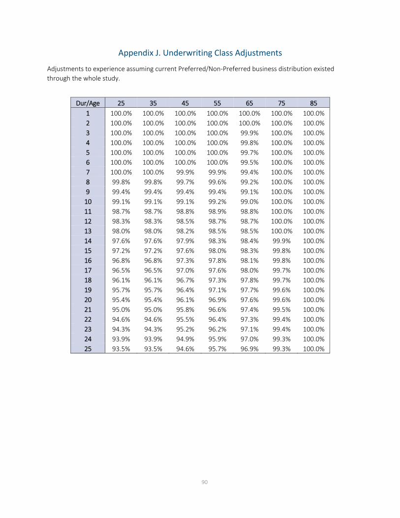
90

Appendix J. Underwriting Class Adjustments

Adjustments to experience assuming current Preferred/Non-Preferred business distribution existed through the whole study.

Dur/Age 25 35 45 55 65 75 85

1 100.0% 100.0% 100.0% 100.0% 100.0% 100.0% 100.0% 2 100.0% 100.0% 100.0% 100.0% 100.0% 100.0% 100.0% 3 100.0% 100.0% 100.0% 100.0% 99.9% 100.0% 100.0% 4 100.0% 100.0% 100.0% 100.0% 99.8% 100.0% 100.0% 5 100.0% 100.0% 100.0% 100.0% 99.7% 100.0% 100.0% 6 100.0% 100.0% 100.0% 100.0% 99.5% 100.0% 100.0% 7 100.0% 100.0% 99.9% 99.9% 99.4% 100.0% 100.0% 8 99.8% 99.8% 99.7% 99.6% 99.2% 100.0% 100.0% 9 99.4% 99.4% 99.4% 99.4% 99.1% 100.0% 100.0%

10 99.1% 99.1% 99.1% 99.2% 99.0% 100.0% 100.0% 11 98.7% 98.7% 98.8% 98.9% 98.8% 100.0% 100.0% 12 98.3% 98.3% 98.5% 98.7% 98.7% 100.0% 100.0% 13 98.0% 98.0% 98.2% 98.5% 98.5% 100.0% 100.0% 14 97.6% 97.6% 97.9% 98.3% 98.4% 99.9% 100.0% 15 97.2% 97.2% 97.6% 98.0% 98.3% 99.8% 100.0% 16 96.8% 96.8% 97.3% 97.8% 98.1% 99.8% 100.0% 17 96.5% 96.5% 97.0% 97.6% 98.0% 99.7% 100.0% 18 96.1% 96.1% 96.7% 97.3% 97.8% 99.7% 100.0% 19 95.7% 95.7% 96.4% 97.1% 97.7% 99.6% 100.0% 20 95.4% 95.4% 96.1% 96.9% 97.6% 99.6% 100.0% 21 95.0% 95.0% 95.8% 96.6% 97.4% 99.5% 100.0% 22 94.6% 94.6% 95.5% 96.4% 97.3% 99.4% 100.0% 23 94.3% 94.3% 95.2% 96.2% 97.1% 99.4% 100.0% 24 93.9% 93.9% 94.9% 95.9% 97.0% 99.3% 100.0% 25 93.5% 93.5% 94.6% 95.7% 96.9% 99.3% 100.0%

91

Appendix K. Calculation of Age-Last-Birthday (ALB) Rates

Below are example calculations showing how age-last-birthday (ALB) mortality rates were developed from the corresponding age-nearest birthday (ANB) rates. Please note that these calculations were originally performed on unrounded numbers. If the rounded, published numbers are used as inputs to replicate the calculations, in some cases the result will be slightly different than those in the published 2015 tables when rounded to two decimal places.

The mortality rates in the below examples are per person; they are equal to the rates displayed in the published tables divided by 1,000.

Example #1 (standard): Calculating the 2015 ALB rate for a male nonsmoker age 75, duration 1

𝑞𝑞[𝑥𝑥]𝐴𝐴𝐴𝐴𝐴𝐴 =

𝑞𝑞[𝑥𝑥]𝐴𝐴𝐴𝐴𝐴𝐴 + �1 − 𝑞𝑞[𝑥𝑥]

𝐴𝐴𝐴𝐴𝐴𝐴� ∗ 𝑞𝑞[𝑥𝑥+1]𝐴𝐴𝐴𝐴𝐴𝐴

2 − 𝑞𝑞[𝑥𝑥]𝐴𝐴𝐴𝐴𝐴𝐴

𝑞𝑞[75]𝐴𝐴𝐴𝐴𝐴𝐴 = 0.00382

𝑞𝑞[76]𝐴𝐴𝐴𝐴𝐴𝐴 = 0.00416

𝑞𝑞[75]𝐴𝐴𝐴𝐴𝐴𝐴 = .00382+(1− .00382)∗ .00416

2− .00382 = 0.00399

Exceptions:

• For age 95, 𝑞𝑞[𝑥𝑥+1]𝐴𝐴𝐴𝐴𝐴𝐴 does not exist in the tables. An artificial age 96 rate was created for this purpose,

calculated as 𝑞𝑞[96]𝐴𝐴𝐴𝐴𝐴𝐴= 4 ∗ 𝑞𝑞[95]

𝐴𝐴𝐴𝐴𝐴𝐴 − 6 ∗ 𝑞𝑞[94]𝐴𝐴𝐴𝐴𝐴𝐴 + 4 ∗ 𝑞𝑞[93]

𝐴𝐴𝐴𝐴𝐴𝐴 − 𝑞𝑞[92]𝐴𝐴𝐴𝐴𝐴𝐴

Example #2: Calculating the 2015 ALB rate for a male nonsmoker age 95, duration 1

𝑞𝑞[96]𝐴𝐴𝐴𝐴𝐴𝐴= 4 ∗ 0.11633− 6 ∗ 0.08149 + 4 ∗ 0.05533− 0.03721 = 0.16046*

𝑞𝑞[95]𝐴𝐴𝐴𝐴𝐴𝐴 = .11633+(1− .11633)∗ .16046

2− .11633 = 0.13703

*when using rounded numbers as shown, the calculation results in 0.16049

• To adjust for the fact that juvenile rates only go through age 17, an artificial age 18 “juvenile” rate was computed as follows to allow for calculation of ALB rates at age 17: 𝑞𝑞[18]𝐴𝐴𝐴𝐴𝐴𝐴= 𝑞𝑞[17]

𝐴𝐴𝐴𝐴𝐴𝐴 + �𝑞𝑞[17]𝐴𝐴𝐴𝐴𝐴𝐴 − 𝑞𝑞[16]

𝐴𝐴𝐴𝐴𝐴𝐴�+ �𝑞𝑞[17]𝐴𝐴𝐴𝐴𝐴𝐴 − 𝑞𝑞[16]

𝐴𝐴𝐴𝐴𝐴𝐴� − (𝑞𝑞[16]𝐴𝐴𝐴𝐴𝐴𝐴 − 𝑞𝑞[15]

𝐴𝐴𝐴𝐴𝐴𝐴)

92

Example #3: Calculating the 2015 ALB rate for a male nonsmoker age 17, duration 1 𝑞𝑞[18]𝐴𝐴𝐴𝐴𝐴𝐴= 0.00057 + (0.00057 − 0.00042) + (0.00057 − 0.00042) − (0.00042 − 0.00029) = 0.00075**

𝑞𝑞[17]𝐴𝐴𝐴𝐴𝐴𝐴 = .00057+(1− .00057)∗ .00075

2− .00057 = 0.00067***

**when using rounded numbers as shown, the calculation results in 0.00074

***when using rounded numbers as shown, the calculation results in 0.00066

93

Appendix L. Mortality Improvement Factors

Attained Age Males Females

Attained Age Males Females

Attained Age Males Females

0 0.0175 0.0110 40 0.0115 0.0075 80 0.0115 0.00751 0.0175 0.0110 41 0.0115 0.0075 81 0.0115 0.00692 0.0175 0.0110 42 0.0115 0.0075 82 0.0115 0.00633 0.0175 0.0110 43 0.0115 0.0075 83 0.0106 0.00584 0.0175 0.0110 44 0.0115 0.0075 84 0.0097 0.00525 0.0175 0.0110 45 0.0115 0.0075 85 0.0088 0.00466 0.0175 0.0110 46 0.0115 0.0075 86 0.0080 0.00407 0.0175 0.0110 47 0.0115 0.0075 87 0.0071 0.00358 0.0175 0.0110 48 0.0115 0.0075 88 0.0062 0.00299 0.0175 0.0110 49 0.0115 0.0075 89 0.0053 0.0023

10 0.0175 0.0110 50 0.0115 0.0075 90 0.0044 0.001711 0.0175 0.0110 51 0.0115 0.0075 91 0.0035 0.001212 0.0175 0.0110 52 0.0115 0.0075 92 0.0027 0.000613 0.0165 0.0104 53 0.0115 0.0075 93 0.0018 0.000014 0.0155 0.0098 54 0.0115 0.0075 94 0.0009 0.000015 0.0145 0.0093 55 0.0115 0.0075 95 0.0000 0.000016 0.0135 0.0087 56 0.0115 0.0075 96 0.0000 0.000017 0.0125 0.0081 57 0.0115 0.0075 97 0.0000 0.000018 0.0115 0.0075 58 0.0115 0.0075 98 0.0000 0.000019 0.0115 0.0075 59 0.0115 0.0075 99 0.0000 0.000020 0.0115 0.0075 60 0.0115 0.0075 100 0.0000 0.000021 0.0115 0.0075 61 0.0115 0.0075 101 0.0000 0.000022 0.0115 0.0075 62 0.0115 0.0075 102 0.0000 0.000023 0.0115 0.0075 63 0.0115 0.0075 103 0.0000 0.000024 0.0115 0.0075 64 0.0115 0.0075 104 0.0000 0.000025 0.0115 0.0075 65 0.0115 0.0075 105 0.0000 0.000026 0.0115 0.0075 66 0.0115 0.0075 106 0.0000 0.000027 0.0115 0.0075 67 0.0115 0.0075 107 0.0000 0.000028 0.0115 0.0075 68 0.0115 0.0075 108 0.0000 0.000029 0.0115 0.0075 69 0.0115 0.0075 109 0.0000 0.000030 0.0115 0.0075 70 0.0115 0.0075 110 0.0000 0.000031 0.0115 0.0075 71 0.0115 0.0075 111 0.0000 0.000032 0.0115 0.0075 72 0.0115 0.0075 112 0.0000 0.000033 0.0115 0.0075 73 0.0115 0.0075 113 0.0000 0.000034 0.0115 0.0075 74 0.0115 0.0075 114 0.0000 0.000035 0.0115 0.0075 75 0.0115 0.0075 115 0.0000 0.000036 0.0115 0.0075 76 0.0115 0.0075 116 0.0000 0.000037 0.0115 0.0075 77 0.0115 0.0075 117 0.0000 0.000038 0.0115 0.0075 78 0.0115 0.0075 118 0.0000 0.000039 0.0115 0.0075 79 0.0115 0.0075 119 0.0000 0.0000

94

About The Society of Actuaries

The Society of Actuaries (SOA), formed in 1949, is one of the largest actuarial professional organizations in the world dedicated to serving 24,000 actuarial members and the public in the United States, Canada and worldwide. In line with the SOA Vision Statement, actuaries act as business leaders who develop and use mathematical models to measure and manage risk in support of financial security for individuals, organizations and the public.

The SOA supports actuaries and advances knowledge through research and education. As part of its work, the SOA seeks to inform public policy development and public understanding through research. The SOA aspires to be a trusted source of objective, data-driven research and analysis with an actuarial perspective for its members, industry, policymakers and the public. This distinct perspective comes from the SOA as an association of actuaries, who have a rigorous formal education and direct experience as practitioners as they perform applied research. The SOA also welcomes the opportunity to partner with other organizations in our work where appropriate.

The SOA has a history of working with public policymakers and regulators in developing historical experience studies and projection techniques as well as individual reports on health care, retirement, and other topics. The SOA’s research is intended to aid the work of policymakers and regulators and follow certain core principles:

Objectivity: The SOA’s research informs and provides analysis that can be relied upon by other individuals or organizations involved in public policy discussions. The SOA does not take advocacy positions or lobby specific policy proposals.

Quality: The SOA aspires to the highest ethical and quality standards in all of its research and analysis. Our research process is overseen by experienced actuaries and non-actuaries from a range of industry sectors and organizations. A rigorous peer-review process ensures the quality and integrity of our work.

Relevance: The SOA provides timely research on public policy issues. Our research advances actuarial knowledge while providing critical insights on key policy issues, and thereby provides value to stakeholders and decision makers.

Quantification: The SOA leverages the diverse skill sets of actuaries to provide research and findings that are driven by the best available data and methods. Actuaries use detailed modeling to analyze financial risk and provide distinct insight and quantification. Further, actuarial standards require transparency and the disclosure of the assumptions and analytic approach underlying the work.

SOCIETY OF ACTUARIES 475 N. Martingale Road, Suite 600

Schaumburg, Illinois 60173 www.SOA.org