2015-06 Engineering of nanoscale antifouling and ...

Calhoun: The NPS Institutional Archive

Theses and Dissertations Thesis Collection

2015-06

Engineering of nanoscale antifouling

and hydrophobic surfaces on naval

structural steel HY-80 by anodizing

Samaras, Thomas

Monterey, California: Naval Postgraduate School

http://hdl.handle.net/10945/45934

NAVAL POSTGRADUATE

SCHOOL MONTEREY, CALIFORNIA

THESIS

Approved for public release; distribution is unlimited

ENGINEERING OF NANOSCALE ANTIFOULING AND HYDROPHOBIC SURFACES ON NAVAL STRUCTURAL

STEEL HY-80 BY ANODIZING

by

Thomas Samaras

June 2015

Thesis Advisor: Co-Advisor:

Sarath K. Menon Claudia C. Luhrs

THIS PAGE INTENTIONALLY LEFT BLANK

i

REPORT DOCUMENTATION PAGE Form Approved OMB No. 0704–0188 Public reporting burden for this collection of information is estimated to average 1 hour per response, including the time for reviewing instruction, searching existing data sources, gathering and maintaining the data needed, and completing and reviewing the collection of information. Send comments regarding this burden estimate or any other aspect of this collection of information, including suggestions for reducing this burden, to Washington headquarters Services, Directorate for Information Operations and Reports, 1215 Jefferson Davis Highway, Suite 1204, Arlington, VA 22202-4302, and to the Office of Management and Budget, Paperwork Reduction Project (0704-0188) Washington, DC 20503. 1. AGENCY USE ONLY (Leave blank)

2. REPORT DATE June 2015

3. REPORT TYPE AND DATES COVERED Master’s Thesis

4. TITLE AND SUBTITLE ENGINEERING OF NANOSCALE ANTIFOULING AND HYDROPHOBIC SURFACES ON NAVAL STRUCTURAL STEEL HY-80 BY ANODIZING

5. FUNDING NUMBERS

6. AUTHOR(S) Thomas Samaras

7. PERFORMING ORGANIZATION NAME(S) AND ADDRESS(ES)Naval Postgraduate School Monterey, CA 93943-5000

8. PERFORMING ORGANIZATION REPORT NUMBER

9. SPONSORING /MONITORING AGENCY NAME(S) AND ADDRESS(ES)N/A

10. SPONSORING/MONITORING AGENCY REPORT NUMBER

11. SUPPLEMENTARY NOTES The views expressed in this thesis are those of the author and do not reflect the official policy or position of the Department of Defense or the U.S. Government. IRB Protocol number ____N/A____.

12a. DISTRIBUTION / AVAILABILITY STATEMENT Approved for public release; distribution is unlimited

12b. DISTRIBUTION CODE

13. ABSTRACT (maximum 200 words)

The impact that biofouling has on a ship’s performance has long been recognized, since it increases the frictional resistance of the hull and can increase the ship’s fuel consumption.

In this study, the spectrum of hydrophobic and antifouling surface patterns that can electrochemically be fabricated on HY-80 steel (alloy that is broadly used in shipbuilding for welded hull plates) is examined. After the fabrication of nanoscaled topographies, the optimum conditions for anodizing are determined by correlating the processing conditions with microstructural data. Characterization of the surface oxides was conducted by techniques such as Scanning Electron and Focused Ion Beam microscopy as well as identification of the formed phases by X-ray diffraction techniques.

Hydrophobicity of the surfaces was examined by measuring the contact angle of deionized water on the HY-80 steel surface. These studies revealed the improved wetting behavior of the anodized surfaces. Thermogravimetric analysis along with quantitative examination of the biofouling on the specimens were studied after prolonged exposure to seawater and indicated a decrease in the corrosion rate of anodized surfaces.

14. SUBJECT TERMS steel, HY-80, anodization, biofouling, hydrophobic, anticorrosion, nanoporous

15. NUMBER OF PAGES

113 16. PRICE CODE

17. SECURITY CLASSIFICATION OF REPORT

Unclassified

18. SECURITY CLASSIFICATION OF THIS PAGE

Unclassified

19. SECURITY CLASSIFICATION OF ABSTRACT

Unclassified

20. LIMITATION OF ABSTRACT

UU NSN 7540–01-280-5500 Standard Form 298 (Rev. 2–89) Prescribed by ANSI Std. 239–18

ii


iii

Approved for public release; distribution is unlimited

ENGINEERING OF NANOSCALE ANTIFOULING AND HYDROPHOBIC SURFACES ON NAVAL STRUCTURAL STEEL HY-80 BY ANODIZING

Thomas Samaras Lieutenant, Hellenic Navy

B.S., Hellenic Naval Academy, 2004

Submitted in partial fulfillment of the requirements for the degree of

MASTER OF SCIENCE IN MECHANICAL ENGINEERING

from the

NAVAL POSTGRADUATE SCHOOL June 2015

Author: Thomas Samaras

Approved by: Sarath K. Menon Thesis Advisor

Claudia C. Luhrs Co-Advisor

Garth V. Hobson Chair, Department of Mechanical and Aerospace Engineering

iv


v

ABSTRACT

The impact that biofouling has on a ship’s performance has long been

recognized, since it increases the frictional resistance of the hull and can

increase the ship’s fuel consumption.

In this study, the spectrum of hydrophobic and antifouling surface patterns

that can electrochemically be fabricated on HY-80 steel (alloy that is broadly

used in shipbuilding for welded hull plates) is examined. After the fabrication of

nanoscaled topographies, the optimum conditions for anodizing are determined

by correlating the processing conditions with microstructural data.

Characterization of the surface oxides was conducted by techniques such as

Scanning Electron and Focused Ion Beam microscopy as well as identification of

the formed phases by X-ray diffraction techniques.

Hydrophobicity of the surfaces was examined by measuring the contact

angle of deionized water on the HY-80 steel surface. These studies revealed the

improved wetting behavior of the anodized surfaces. Thermogravimetric analysis

along with quantitative examination of the biofouling on the specimens were

studied after prolonged exposure to seawater and indicated a decrease in the

corrosion rate of anodized surfaces.

vi


vii

TABLE OF CONTENTS

I. INTRODUCTION ............................................................................................. 1 A. MOTIVATION ....................................................................................... 1 B. LITERATURE REVIEW ON ANODIZATION ....................................... 3 C. OBJECTIVES ....................................................................................... 4 D. THESIS TASKS ................................................................................... 5

II. BACKGROUND .............................................................................................. 7 A. BIOFOULING MECHANISMS ............................................................. 7 B. APPLICATIONS AND PROPERTIES OF NAVAL STEEL HY-80 ....... 8 C. PRINCIPLE OF ANODIZATION......................................................... 10

III. MATERIALS AND CHARACTERIZATION METHODS ................................ 13 A. MATERIALS ...................................................................................... 13

1. Steel Samples ........................................................................ 13 2. Chemical Reagents ................................................................ 16 3. Lab Ware (Glassware and Metalware) .................................. 16

B. CHARACTERIZATION METHODS .................................................... 16 1. Scanning Electron Microscopy (SEM) ................................. 16 2. Energy-Dispersive X-ray Spectroscopy (EDS) .................... 19 3. X-ray Diffractometry/Diffractometer (XRD) .......................... 19 4. Focused Ion Beam (FIB) ........................................................ 21 5. Differential Scanning Calorimeter (DSC) and Thermal

Gravimetric Analysis (TGA) .................................................. 23 6. Contact Angle Measurement ................................................ 26 7. Corrosion Rate Measurement ............................................... 27

IV. EXPERIMENTAL PROCEDURES ................................................................ 29 A. NAOH-BASED ELECTROLYTE ........................................................ 30 B. NH4F-BASED ELECTROLYTE .......................................................... 33

1. 0.50 wt% NH4F, 3 wt% DI Water ............................................ 33 2. 0.37 wt% NH4F, 1.8 wt% DI Water ......................................... 33 3. 0.37 wt% NH4F, 0.9 wt% DI Water ......................................... 33

V. RESULTS & DISCUSSION ........................................................................... 35 A. CHARACTERIZATION WITH SEM .................................................... 35 B. GROWTH KINETICS OF NANOPOROUS ANODIC FILMS .............. 47 C. CHARACTERIZATION WITH EDS .................................................... 51 D. CHARACTERIZATION WITH XRD .................................................... 55 E. CHARACTERIZATION WITH FIB ...................................................... 63 F. CONTACT ANGLES .......................................................................... 65 G. CORROSION RESISTANCE ............................................................. 67 H. BIOFOULING ..................................................................................... 69

1. Thermal Analysis ................................................................... 69 2. SEM/EDS Analysis ................................................................. 73

viii

VI. CONCLUSIONS ............................................................................................ 83

VII. FUTURE WORK ........................................................................................... 85

LIST OF REFERENCES .......................................................................................... 87

INITIAL DISTRIBUTION LIST ................................................................................. 91

ix

LIST OF FIGURES

Figure 1. Schematic of biofouling stages on steel substrate, from [30] ................ 8 Figure 2. Schematic of a typical anodization setup ............................................ 11 Figure 3. EDS spectrum from HY-80 steel......................................................... 14 Figure 4. Struers Secotom-10 table-top precision cut-off machine .................... 15 Figure 5. Ecomet 4 (left) and Ecomet 3 (right) automatic polishers ................... 15 Figure 6. Specimen interaction with electron beam, from [38] ........................... 17 Figure 7. The Scanning Electron Microscopy setup .......................................... 17 Figure 8. DC magnetron High Resolution Sputter Coater .................................. 18 Figure 9. Vacuum chamber (on left) and dual-seal vacuum pump (on right) by

Welch Manufacturing Co. (Chicago, IL) .............................................. 19 Figure 10. Rigaku Miniflex 600 X-ray Diffractometer ........................................... 20 Figure 11. Principles of FIB: (a) imaging (b) sputtering–milling (c) deposition,

from [41] ............................................................................................. 22 Figure 12. Diagram of NETZSCH STA 449 F3 Jupiter DSC/TGA (top) and

picture of setup in NPS laboratory (bottom), from [43] ........................ 24 Figure 13. Diagram of NETZSCH TA-QMS 403C Aėolos QMS (left) and

picture of setup in NPS laboratory (right), from [43]............................ 25 Figure 14. TGA/DSC coupled with the quadruple mass spectrometer (QMS) ..... 25 Figure 15. Dino Lite optical microscope ............................................................... 26 Figure 16. Contact angle measurement, where θc is the contact angle, and γsl,

γsv, and γlv are the solid–liquid, solid–vapor and liquid–vapor interfaces, respectively ....................................................................... 27

Figure 17. Dhaus Adventurer Pro micro balance ................................................. 28 Figure 18. Picture of the ultrasonic cleaner ......................................................... 30 Figure 19. A photograph of the general anodization set up: (a) power supply,

(b) multimeter/alternative power source, (c) multimeter, (d) heating plate, (e) temperature controller (f) galvanic cell ................................ 31

Figure 20. Annealing plot ..................................................................................... 32 Figure 21. SEM images of anodized steel surfaces under 5 min anodization in

50 wt% NaOH solution under 2.5 V (left) and 12.5V (right) at 75 °C .. 35 Figure 22. SEM images of (a) nanoporous channels, (b) spherical, and (c)

hexagonal crystal structures on anodized steel surfaces under 5 min, 12.5 V anodization in 50 wt% NaOH solution ............................. 36

Figure 23. Image of a “collapsed” hump on the surface of a 5 min, 2.5 V, at 90 °C anodized steel in 50 wt% NaOH solution ....................................... 37

Figure 24. SEM images showing the pitting effect on the surface of anodized HY-80 steel under potentials of (a) 10 V,(b) 25 V, (c) 30 V, and (d) 50 V .................................................................................................... 38

Figure 25. SEM image of steel surface under 10 min, 50 V anodization in 0.50 wt% NH4F, 3 wt% DI water EG solution at 60 °C ................................ 38

x

Figure 26. SEM images of anodized sample in 10 V, 60 °C, 0.50 wt% NH4F, 3 wt% DI water in EG electrolyte under (a) low, (b) medium, and (c) high magnification............................................................................... 39

Figure 27. SEM images of anodized sample in 25 V, 60 °C, 0.50 wt% NH4F, 3 wt% DI water in EG electrolyte under (a) low and (b) high magnification ...................................................................................... 40

Figure 28. SEM images of anodized sample in 40 V, 60 °C, 0.50 wt% NH4F, 3 wt% DI water in EG electrolyte focusing on (a) nano porous and (b) nano channeling structure .................................................................. 40

Figure 29. SEM macroscopic images of anodized sample in 50 V, 60 °C, 0.50 wt% NH4F, 3 wt% DI water in EG electrolyte ...................................... 41

Figure 30. SEM images on high (left) and low (right) magnification of nanoporous structure under 1 h anodization in a 0.37 wt% NH4F, 1.8 wt% DI water EG solution on 20 V at 25 °C .................................. 42




Figure 34. SEM images of nanoporous structure under 5 min (left) or 15 min (right) anodization in a 0.37 wt% NH4F, 0.9 wt% DI water EG solution with applied current density of 30A/m2 at 25 °C .................... 44

Figure 35. SEM images of nanoporous structure under 5 min (left) or 15 min (right) anodization in a 0.37 wt% NH4F, 0.9 wt% DI water EG solution with applied current density of 45A/m2 at 25 °C .................... 44

Figure 36. SEM images of nanoporous structure under 5 min anodization in a 0.37 wt% NH4F, 0.9 wt% DI water EG solution with applied current density of 85A/m2 at 25 °C ................................................................. 45

Figure 37. SEM image on a 5 min anodized surface under 85A/m2 .................... 45 Figure 38. SEM images on a lower magnification of samples anodized for 15

min at 60 A/m2 (top) and 85A/m2 (bottom) .......................................... 46 Figure 39. Current density versus time curve recorded during anodization in

0.37 wt% NH4F, 1.8 wt% DI water EG solution at 25 °C during various time intervals .......................................................................... 48

Figure 40. Potential density versus time curve recorded during 5 min anodization in 0.37 wt% NH4F, 0.9 wt% DI water EG solution at 25 °C ....................................................................................................... 51

Figure 41. Potential density versus time curve recorded during 15 min anodization in 0.37 wt% NH4F, 0.9 wt% DI water EG solution at 25 °C ....................................................................................................... 51

xi

Figure 42. EDS spectrum from the spherical structure oxide on anodized steel surface after 5 min in a 50 wt% NaOH solution with applied voltage of 2.5 V at 75 °C ................................................................................. 52

Figure 43. EDS spectrum from the hexagonal structure oxide on anodized steel surface after 5 min in a 50 wt% NaOH solution with applied voltage of 2.5 V at 75 °C ..................................................................... 53

Figure 44. EDS spectra from anodized steel after 1 hour in a 0.37 wt% NH4F, 1.8 wt% DI water EG solution with applied voltage of 20 V at room temperature ........................................................................................ 54

Figure 45. EDS spectra from anodized steel after 5 min in a 0.37 wt% NH4F, 0.9 wt% DI water EG solution with applied current density of 40A/m2 at room temperature .............................................................. 54

Figure 46. XRD patterns of the iron oxide created after 5 min anodization in 7.5 V, 75 °C, in a 50 wt% NaOH solution before (top) and after (bottom) annealing.............................................................................. 57

Figure 47. XRD patterns of the iron oxide created after 5 min anodization in 12.5 V, 75 °C, in a 50 wt% NaOH solution before (top) and after (bottom) annealing.............................................................................. 58

Figure 48. XRD patterns of the iron oxide created after 5 min anodization in 30 V, 50 °C, in a 0.50 wt% NH4F, 3 wt% DI water EG solution before (top) and after (bottom) annealing ...................................................... 59

Figure 49. XRD patterns of the iron oxide created after 5 min anodization in 50 V, 50 °C, in a 0.50 wt% NH4F, 3 wt% DI water EG solution before (top) and after (bottom) annealing ...................................................... 60

Figure 50. XRD patterns of the iron oxide created after 60 min anodization in 30 V, 25 °C, in a 0.37 wt% NH4F, 1.8 wt% DI water EG solution before (top) and after (bottom) annealing ........................................... 61

Figure 51. XRD patterns of the iron oxide created after 15 min anodization in 45A/m2, 25 °C, in a 0.37 wt% NH4F, 0.9 wt% DI water EG solution before (top) and after (bottom) annealing ........................................... 62

Figure 52. FIB image of anodized steel surface under current density of 40 A/m2 in EG solution of 0.37 wt% NH4F, 0.9 wt% DI water concentration, for 5 min ...................................................................... 64

Figure 53. FIB image of anodized steel surface under current density of 45 A/m2 in EG solution of 0.37 wt% NH4F, 0.9 wt% DI water concentration, for 15 min .................................................................... 64

Figure 54. Histogram of contact angles for plain steel ......................................... 65 Figure 55. Pictures of contact angles (a) on the surface of polished steel, and

on the surfaced of anodized steels under (b) NaOH electrolyte in 7.5 V, 75 °C for 5 min, (c) 0.50 wt% NH4F, 3 wt% DI water, EG electrolyte in 50 V, 60 °C for 5 min, (d) 0.37 wt% NH4F, 1.8 wt% DI water, EG electrolyte in 30 V, room temperature for 1 hour, and (e) 0.37 wt% NH4F, 0.9 wt% DI water, EG electrolyte in 45.2 A/m², room temperature for 5 min ................................................................ 67

Figure 56. TGA analysis ...................................................................................... 70

xii

Figure 57. DSC analysis ...................................................................................... 71 Figure 58. TGA/QMS diagram ............................................................................. 72 Figure 59. EDS spectrum from the iron oxide formed on the surface of

polished steel plate left in DI water–3.5wt% NaCl solution for 10 days .................................................................................................... 75

Figure 60. SEM images of calcium carbonate (CaCO3) crystals with their corresponding dimensions appearing in red lines .............................. 76

Figure 61. SEM images of aragonite crystal in low (left) and high (right) magnification ...................................................................................... 77

Figure 62. EDS spectrum from a calcium carbonate (CaCO3) crystal ................. 77 Figure 63. EDS spectrum from corroded steel plate in seawater ......................... 79 Figure 64. SEM images of various crystalline forms of CaCO3 crystals such as

calcite in (a) and aragonite in (b) and (c), from [46] ........................... 81

xiii

LIST OF TABLES

Table 1. Chemical composition of HY-80 steel, after [33] ................................... 9 Table 2. Mechanical properties of HY-80, after [32, 34] ................................... 10 Table 3. Physical properties of HY-80, after [35] .............................................. 10 Table 4. Elemental composition of steel sample analyzed at Anamet, Inc ....... 13 Table 5. EDS quantitative analysis showing weight and atomic number

percent of elements in HY-80 steel .................................................... 14 Table 6. Summary of the applied anodization methods .................................... 34 Table 7. EDS quantitative analysis showing weight and atomic number

percent of elements in anodized steel area of Figure 42 .................... 52 Table 8. EDS quantitative analysis showing weight and atomic number

percent of elements in anodized steel area of Figure 43 .................... 53 Table 9. EDS quantitative analysis showing weight and atomic number

percent of elements in the Figure 44 anodized steel .......................... 54 Table 10. EDS quantitative analysis showing weight and atomic number

percent of elements in the Figure 45 anodized steel .......................... 55 Table 11. Contact angles of DI water on the surface of anodized steel under

NaOH electrolyte ................................................................................ 66 Table 12. Contact angles of DI water on the surface of anodized steel under

various EG-based electrolytes ............................................................ 67 Table 13. Corrosion rates for HY-80 ................................................................... 68 Table 14. EDS quantitative analysis showing weight and atomic number

percent of elements of iron oxide appearing in Figure 59 ................... 76 Table 15. EDS quantitative analysis showing weight and atomic number

percent of elements of the CaCO3 crystal in Figure 62 ....................... 79 Table 16. EDS quantitative analysis showing weight and atomic number

percent of elements appearing in the corroded steel surface of Figure 63 ............................................................................................ 80

xiv


xv

LIST OF ACRONYMS AND ABBREVIATIONS

A Ampere

Al Aluminum

At% Atomic Number Percent

BSE Backscattered Electrons

C Carbon

Cr Chromium

cm Centimeters

Cu Copper

DI Deionized Water

DSC Differential Scanning Calorimeter

e- Electron

EG Ethylene Glycol

EDS Energy-dispersive X-ray Spectroscopy

EPS Extracellular Polymeric Substances

Fe Iron

FIB Focused Ion Beam

h Hour

H Hydrogen

H2SO4 Sulfuric Acid

HClO4 Perchloric Acid

HF Hydrofluoric Acid

ICDD International Centre for Diffraction Data

KOH Potassium Hydroxide

KV Kilovolts

LMIS Liquid Metal Ion Source

m Meter

mg Milligram

Mg Magnesium

xvi

min Minute

ml Milliliter

mm Millimeter

Mn Manganese

Mo Molybdemun

MPY Mils Penetration per Year

nA Nano Amperes

NaCl Sodium Chloride

NaOH Sodium Hydroxide

NH4F Ammonium Fluoride

Ni Nickel

nm Nanometers

NPS Naval Postgraduate School

P Phosphorous

pA Pico Amperes

QMS Quadruple Mass Spectrometer

S Sulfur

SE Secondary Electrons

sec Second

SEM Scanning Electron Microscopy/Microscope

Si Silicon

SiC Silicon Carbide

Ta Tantalum

TGA Thermogravimetric Analysis

TBT Tributyltin

TBTO Tributyltin Oxide

Ti Titanium

rpm Revolutions per Minute

V Volts

wt% Weight Percent

xvii

w/v Weight over Volume

XRD X-ray Diffractometry/Diffractometer

Zr Zirconium

µl Microliter

µm Micrometer

xviii


xix

ACKNOWLEDGMENTS

I dedicate this work to my wife, Betty, for her continuous loving support

and patience, and to my newborn son for the happiness that he brought to my

life.

This thesis would not have been possible without the invaluable support

and wise guidance of my thesis advisor Professor Sarath Menon and co-advisor

Claudia Luhrs. Both their professionalism and their wealth of knowledge shined

like a beacon leading the way. Sincerely, I couldn’t have asked for more

compassionate individuals as supervisors and I consider myself enlightened after

having been their student.

I would also like to deeply thank all my friends and classmates for listening

to me droning on about my thesis and for being there when I needed them the

most. Wei Zhong and Nazmi, I wish you both the best of luck on your future

endeavors.

Lastly and most importantly, I would like to thank the Hellenic Navy for

believing in me and providing me with the opportunity to make a lifetime dream

come true and study at one of the most prominent universities.

xx


1

I. INTRODUCTION

A. MOTIVATION

One of the major concerns in naval engineering has been the marine

biofouling caused by the adhesion of living organisms in submerged seawater

surfaces, whether on ship hulls, pipelines, or even marine structures such as

platforms or bridge pillars. The negative effects that biofouling has on a ship’s

hull include the following: (i) bio corrosion that increases the chances of crevice

corrosion, which can be devastating to the structure by resulting in premature

structural failure, (ii) extensive maintenance, and (iii) increase of the surface

roughness which in turn causes an increase in hydrodynamic drag and,

therefore, an increase in the frictional resistance of the ship. Frictional resistance

can account for as much as 90% of the ship’s total drag [1] and, subsequently,

this results in an approximately 40% increase to the ship’s fuel consumption [2]

or even the reduction of a ship’s maximum speed up to 2 knots [3]. This has a

tremendous economic impact, calculated in 2010 to be $2.3 million per ship in

the U.S. Navy alone [1].

From ancient times, people have struggled with microbial attachment to

vessels and since the origins of naval engineering, innovative methods have

been used to overcome these problems. Ancient Phoenicians and Carthaginians

used wax, tar, and asphalt, and there is even a record of arsenic and sulfur being

used in 412 BC. These methods were used up until copper became the first

successful antifouling surface to receive worldwide recognition [3].

Nowadays, the best established antifouling methods are “paints.” Recent

studies indicated that widely used organotin compounds such as tributyltin (TBT)

and tributyltin oxide (TBTO) have been found to be toxic to marine organisms

that are not related to biofouling [4], and subsequently their use has been

forbidden from the Marine Environment Protection Committee of the International

Maritime Organization [5]. Therefore, modern naval engineering is seeking new,

2

environmentally friendly ways of reducing biofouling. Novel approaches include

increasing the ship surface’s antifouling properties by increasing its

hydrophobicity. A lot of research is being conducted in constructing micro or

nano scale patterned surfaces that reduce wettability, and nano scale patterns

were manufactured that can decrease biological fouling from 47% up to 86% [6,

7].

The development of biomimetic or bio-inspired materials has been

suggested as a means to reduce barnacle attachment, and research in this area

appears very promising. Studies on bio-inspired micro scale topographically

rough surfaces for antifouling purposes have received a lot of interest, given the

observation of reduced barnacle settlement on shark skin. The surface of the

shark skin has grooves and fine scales (dermal denticles), and these features

have inspired scientists to develop techniques based on lithographic patterning to

reproduce similar artificial structures that are hydrophobic, which aid in the

deterrence of bio-organism colonization as well [7, 8].

One of the techniques suggested by previous Naval Postgraduate School

(NPS) studies to create hydrophobic/antifouling surfaces is anodization. This

technique has been successful on aluminum [9], titanium [10] and their alloys

indicating that this very simple and well-established method can provide

extremely useful results in various applications such as energy storage materials,

bio sensing, orthopedics [11, 12], and so forth. The hydrophobicity of anodized

nanoporous structures has been reported, and the role of wettability in impeding

biofouling, including barnacle attachment on surfaces, is well recognized [13].

Through a two-step high field anodization in phosphoric acid, J.C. Buijnsters et

al[9]. produced 5 μm thick nanoporous anodized aluminum oxide films with

average pore openings in the range of 140–190 nm, which reduced the

wettability of aluminum alloy 1050 from approximately 92o [14] up to 128o. In the

case of titanium, studies of P.V. Mahalakshmi et al. [10] indicated that precoating

treatment by anodization in sulfuric acid (H2SO4) and hydrofluoric acid (HF)

electrolyte bath for 1h at 30 V led to the development of super hydrophobic

3

titanium surfaces with contact angles of 1480 ± 40 and increased microbial

attachment resistance.

Metal anodizing techniques have been widely used to modify surfaces.

Moreover, because the process increases corrosion and wear resistance and

can also be applied to large marine structures, the technique is more appealing

for applications in the shipbuilding industry than the patterning techniques.

B. LITERATURE REVIEW ON ANODIZATION

In the last decades, there have been plenty of reports on self-ordering

electrochemical processes to prepare highly ordered oxide nanostructures. The

majority of these studies focus on metals such as Al, Ti, Zr, and Ta [10, 15–18].

However, the self-organized porous alumina arrays grown by anodization on

either pure aluminum or aluminum alloys represent the most studied system [9,

19–21].

Although iron is a widely used metal, only a few attempts can be found to

electrochemically fabricate ordered oxide nanostructures on the surface of Fe-

based metals.

Burleigh et al. published two reports in 2007 [22] and 2009 [23], followed

by a patent in 2011 [24], presenting a novel method of anodizing steel in 10 wt%

to saturated solutions of potassium hydroxide (KOH) and sodium hydroxide

(NaOH). They produced anodized films consisting mainly of magnetite (Fe3O4) in

both solutions (KOH and NaOH) that provide improved corrosion protection to

steel.

The majority of studies on steel and iron anodization, though, focus on an

ethylene glycol (EG)–based electrolyte containing dissolved ammonium fluoride

(NH4F) in deionized water (DI). Keyu Xie et al. [25] published extensive research

on fabricating iron oxide (hematite) nanotubes on Fe foils through

electrochemical anodization at an applied voltage between 30–50 V, in an EG-

based electrolyte composed of 0.25–0.50 wt% NH4F and 1–3 wt% DI water at

4

elevated temperatures of up to 60 oC. A similar method is also suggested by

Sergiu Albu et al. [26] but with different anodization conditions of temperature,

concentration, and applied voltage.

In a paper by Y. Konno et al. [27], a galvanostatic anodization was

introduced in an EG-based electrolyte containing 0.1M NH4F and 0.5M DI water

in 20 oC that resulted in the formation of self-organized nanoporous anodic films,

but in this case the research had been in done in low carbon steels (instead of Fe

foils).

In a different electrolytic environment that consisted of 3–10 wt%

Perchloric acid (HClO4) and EG, W. Zhan et al. [28] succeeded in creating a 13

nm to 26 nm thickness film of nanoporous arrays on stainless steel by

anodization. The oxide structures produced under these conditions granted the

material significant visible light photo catalytic activities along with corrosion

resistance.

In the research on anodization of Fe-based metal surfaces [22–25, 27,

28], the focus has been on the examination of the morphologies of the

nanoporous structures and the evaluation of the anodization parameters such as

anodization potential, time, temperature, and electrolyte composition on the oxide

layer.

C. OBJECTIVES

The overall aim of this study was to examine the potential of anodized

surfaces on improving the biofouling resistance and corrosion properties of hull

steel. With that in mind, in this preliminary study, the overarching objective was

the fabrication and characterization of nano-topographic structures using

anodization processes on naval steel HY-80. Further objectives are the

evaluation of the wetting and antifouling properties that these surface patterns

may present. If either wettability or antifouling can be achieved through this

simple industrial method, the impact on naval structural engineering will be

profound. However, it must be noted that the anodized steel with iron oxide

5

nanoporous structures is unlikely to provide sufficient metallic corrosion

protection due to the non-adherence of the oxide films. Further modification of

the chemistry of the surface will be necessary for a practical application of this

idea. Nevertheless, the results of this preliminary study will form the backbone for

the further development of structures with sufficient corrosion and prolonged

antifouling protection sufficient to be of practical application in many marine

structures, specifically those of interest to the Navy worldwide.

D. THESIS TASKS

The current thesis study is focused on the following procedures:

The initial aim is the production of homogeneous nanoporous structures, based on the methods proposed by Burleigh et al. [22, 23], Xie et al. [25], Albu et al. [26], and Konno et al. [27] and described in the literature review section. Since most of these reports refer to either anodization of pure iron or generalized steel alloys, appropriate alterations in anodizing parameters are applied in order to reach the desired result.

Characterization will be conducted with scanning electron microscopy (SEM), X-ray diffractometry (XRD), and serial sectioning microstructures by focused ion beam (FIB) microscopy to observe the cross section of anodized products, on selected samples. After making tests with various anodizing techniques and evaluating each sample, expectations are to distinguish the optimum design process and the limitation for each pattern.

Wettability studies are performed by measuring water drop contact angles on the created surfaces, to evaluate its hydrophobic or hydrophilic behavior.

Preliminary corrosion resistance assessment by weight loss measurements of anodized samples in stagnant Monterey seawater will provide information on their anti-corrosive properties. A limited amount of biofouling could be expected under these conditions and will be examined by optical and scanning electron microscopy studies.

Finally, with the use of thermogravimetric analysis (TGA) and SEM quantitative analysis, an examination of the antifouling properties completes this study.

6


7

II. BACKGROUND

A. BIOFOULING MECHANISMS

Biofouling (biological fouling) is defined as the accumulation of living

organisms, such as macro algae, hydrozoans, bryozoans, barnacles, polychaete

tubeworms, mollusks, and ascidians on artificial surfaces by adhesion, growth,

and reproduction. Biofouling can be characterized into two main categories:

micro fouling and macro fouling.

Micro fouling is the initial stage of biofouling and describes the formation

of biofilm organisms, which are bacteria and diatoms on submerged structures.

Biofilms are ubiquitous, as long as surfaces are exposed to seawater [2]. Minutes

after a surface has been submerged in water, it absorbs a molecular film that

consists of dissolved organic material. Within the next few hours, this film is

colonized by bacteria, unicellular algae (especially diatoms), and/or

cyanobacteria (blue-green algae), which together form a biofilm—an assemblage

of attached cells, which is commonly referred to as slime [29].

These microorganisms adhere to the surface by extracellular polymeric

substances (EPS). So the biofilm, which is the result of micro fouling, comprises

both the microorganisms and the EPS, and thus the physical properties of the

surface change, making it more amenable for the settlement of macro-fouling

organisms. Then, the attached cells further divide, giving rise to colonies that

eventually coalesce to form a compact biofilm, which in some cases may even

achieve a thickness of 500 μm [29].

Macro fouling in the submerged surface occurs after two or three weeks,

when micro-fouling organisms finally have evolved into a complex biological

community and have chemically prepared the surface for the settlement of

macro-fouling species. Macro-fouling organisms settle, develop, and overgrow

the micro-fouling surface. The most important macro-fouling species are

barnacles, algae, mussels, polychaete worms, bryozoans, and seaweed [2].

8

A macro-fouling community consists of either soft fouling or hard fouling.

Soft fouling comprises algae and invertebrates, such as soft corals, sponges,

anemones, tunicates, and hydroids, whilst hard fouling comprises invertebrates

such as barnacles, mussels, and tubeworms.

The specific organisms that develop in a fouling community depend on the

substratum, geographical location, season, and factors such as competition and

predation [29]. Fouling is a highly dynamic process; an over-simplified schematic

example of its evolution appears in Figure 1.

Figure 1. Schematic of biofouling stages on steel substrate, from [30]

B. APPLICATIONS AND PROPERTIES OF NAVAL STEEL HY-80

The HY (High Yield) series of steels have been used in U.S. naval

warships since the 1950s. HY-80 steels (military specification MIL-S-16216) are

broadly used in shipbuilding for welded hull plates and structural use, due to their

excellent weldability and notch toughness, along with their good ductility even in

welded sections.

The HY-80 steels are metallurgically classified as quenched and tempered

martensitic steels. They have a martensitic microstructure resulting from the

9

combination of alloying, which can be seen in Table 1, and heat treatment

employment to provide the optimal combination of strength and toughness.

This heat treatment consists of two procedures. The austenization in the

ranges of 844 °C to 899 °C, followed by a water quench, and the tempering in the

range of 621 °C to 677 °C (and in no case less than 600 °C), followed also by a

water quench [31].

Following this heat treatment, the alloy develops a martensitic structure

(the final product should contain more than 80% martensite), which provides to

metal the desired mechanical properties of Table 2 and the physical properties of

Table 3.

The alloying elements promote martensitic formation, but the alloying

element with the major effect in producing a martensitic structure is carbon. The

as-quenched steel manifests high strength and hardness but also is brittle and

susceptible to hydrogen (cold) cracking [32].

Table 1. Chemical composition of HY-80 steel, after [33]

Element (wt%) Carbon (C) 0.10–0.20 Phosphorous (P) 0.020 max Manganese (Mn) 0.010–0.46 Silicon (Si) 0.12–0.38 Sulfer (S) 0.020 max Nickel (Ni) 1.93–3.32 Chromium (Cr) 0.94–1.86 Molybdenum (Mo) 0.17–0.63 Vanadium (V) 0.030 max Titanium (Ti) 0.020 max Copper (Cu) 0.25 max

10

Table 2. Mechanical properties of HY-80, after [32, 34]

Yield strength 552 Mpa Elongation 20% Reduction of area 50%

Charpy impact 81 J at -18 °C and 48 J at -84 °C

Transverse dynamic tear test

610 J at -40 °C

Table 3. Physical properties of HY-80, after [35]

Hardness (Rockwell) C-21 Elastic Properties

Elastic modulus, E 207 (GPa) Poisson’s Ratio, ν 0.30 Shear modulus, E/2 (1+ ν) 79 (GPa) Bulk modulus, E/3 (1-2ν) 172 (GPa)

Thermal Properties Density, ρ 7746 (kg/m3) Conductivity, k 34 (W/mK) Specific heat, cρ 502 (J/kgK) Diffusivity, k/ ρ cρ 9x10-6 (m2/s) Expansion coef. (Vol), α 11x10-6 (K-1) Melting temperature, TMELT 1793 (K)

C. PRINCIPLE OF ANODIZATION

Anodization, or anodic oxidation, is a well-established, low-cost industrial

surface modification process that was discovered back in the early 1930s [12]; it

is an electrochemical process developed not only to improve the native protective

oxide films created on the surface of metals by making them more stable and

highly resistant, but also to modify the surface by giving it a desired morphology.

Ferrous alloys such as HY-80 have a very high chemical affinity for oxygen and

rapidly corrode in aqueous media [36].

11

Iron can be oxidized to different valence states such as FeO, Fe2O3, and

Fe3O4. The typical chemical reaction for anodizing iron in valence state 3 in an

aqueous solution is illustrated below in equations (1) to (5), while an anodization

setup of Fe is shown in Figure 2.

2

2 2H O H O (1)

In the anode: 3 3Fe Fe e (2)

3 2

2 32 3Fe O Fe O (3)

Overall process: 2 2 32 3 6 6Fe H O Fe O H e (4)

In cathode: 26 6 3 ( )H e H gas (5)

Figure 2. Schematic of a typical anodization setup

12


13

III. MATERIALS AND CHARACTERIZATION METHODS

A. MATERIALS

1. Steel Samples

A plate of HY-80 steel was obtained from the Naval Surface Warfare

Center (Carderock Division, Bethesda, MD). A small piece from this plate was

sent for chemical analysis to Anamet, Inc. (Hayward, CA) to determine if the

material procured was in fact HY-80 by composition. Additional elemental

identification was performed using the energy-dispersive X-ray spectroscopy

(EDS) technique to verify that the chemical composition of the samples matched

the chemical composition specifications of HY-80, as previously described in

Table 1. The results, as can be seen in the diagram of Figure 3 and in Tables 4

and 5, corroborate the quality of the samples.

Table 4. Elemental composition of steel sample analyzed at Anamet, Inc

Element Min

(wt%)Max

(wt%)

Carbon (C) --- 0.18 Chromium (Cr) 1.00 1.8 Copper (Cu) --- 0.25 Manganese (Mn) 0.10 0.40 Molybdenum (Mo) 0.20 0.60 Nickel (Ni) 2.00 3.25 Phosphorous (P) --- 0.025*Silicon (Si) 0.15 0.35 Sulfer (S) --- 0.025*

Titanium (Ti) --- 0.02

Vanadium (V) --- 0.03

14

Figure 3. EDS spectrum from HY-80 steel

Table 5. EDS quantitative analysis showing weight and atomic number percent of elements in HY-80 steel

Element Wt% At% Silicon (Si) 00.35 00.71 Chromium (Cr) 01.62 01.73 Manganese (Mn) 00.46 00.46 Iron (Fe) 95.54 95.17 Nickel (Ni) 02.03 01.92 Matrix Correction ZAF

Prior to any experimental procedure, the steel was cut to the desired

dimensions, 17.5 mm × 5.7 mm × 0.8 mm, using the Struers Secotom-10 table-

top precision cut-off machine (Figure 4) with a Struers Alumina cut-off wheel

50A20 (200 mm diameter × 0.8 mm × 22 mm diameter) at 2000 rpm and 30

mm/sec speed.

15

Figure 4. Struers Secotom-10 table-top precision cut-off machine

Grinding and polishing of specimens were conducted on a Buehler

Ecomet 4 automatic polisher (Figure 5) at high speeds (100 rpm) starting with

waterproof silicon carbide paper (SiC) 320 grit and gradually increasing to SiC

800 grit, SiC 1200 grit and SiC 2500 grit. Further polishing was conducted on a

Buehler Ecomet 3 automatic polisher (Figure 5) with Buehler alumina/silica micro

cloth grinding pad, 1 micron sized at moderate speeds. Polishing time for the

most abrasive papers was typically 20 min, and up to 40 min for the finer grit.

Figure 5. Ecomet 4 (left) and Ecomet 3 (right) automatic polishers

16

2. Chemical Reagents

Sodium hydroxide (NaOH) was purchased from EMD Chemical Inc.

(Gibbstown, NJ), and ammonium fluoride (NH4F) and ethylene glycol (EG) 99.8%

were purchased from Aldrich Chemistry (St. Louis, MO). All of the mentioned

reagents were used as received, unless otherwise mentioned.

3. Lab Ware (Glassware and Metalware)

All lab ware (i.e., test tubes, vials, droppers, spatulas, etc.) was cleaned in

a laboratory sink following a regime that involved a detergent wash and a

minimum of three DI water rinses. The DI water was purchased from Weber

Scientific. The detergent wash consisted of commercial dishwasher detergent in

a solution of tap water. Following the cleaning procedure, all glass and metal

ware were left to air dry overnight until use.

B. CHARACTERIZATION METHODS

1. Scanning Electron Microscopy (SEM)

Scanning Electron Microscopy (SEM) is the most widely used type of

electron microscope [37]. In SEM, an electron gun produces a beam of

monochromatic electrons. This beam passes through the condenser lens

producing a coherent beam, which is focused onto the sample surface through

an objective lens. The electron beam thus focused on the specimen is scanned

across the specimen surface [38]. When an electronic beam strikes the

specimen, due to various interactions, a variety of signals are generated, as

shown in Figure 6. From this impact, electrons are emitted as a result of elastic

and inelastic scattering, resulting in backscattered electrons (BSE) and

secondary electrons (SE), respectively. SEM collects these electrons through

detectors, amplifies them, and reconstructs a digital image of the surface of the

specimen. Both signals give useful information in the imaging process with the

SEs to be the primary signals for achieving topographic contrast, and the BSEs

for the formation of elemental composition contrast.

17

Figure 6. Specimen interaction with electron beam, from [38]

A Zeiss Neon 40 Crossbeam Scanning Electron Microscope with a

Schottky type field emission electron source (Figure 7) was used to determine

the topography, morphology, and size distribution of the constructed structures.

Figure 7. The Scanning Electron Microscopy setup

The system was energized to 2 KV and a beam current of 100pA was

found to be ideal to image the anodized steel surface without the need for a

18

conducting metal coating. An exception to this procedure was the preparation of

biofouled samples. To ensure electrical continuity, a requirement for SEM, each

sample was prepared by applying a thin coating layer of Pt20Pd using the DC

magnetron High Resolution Sputter Coater Cressington 208HR with rotary-

planetary-tilt stage thickness controller MTM-20, as seen in Figure 8. Analysis

was conducted using the SmartSEM V05.04.03.00 software package developed

by Carl Zeiss SMT Ltd, and quantitative analysis, when needed, through ImageJ,

a public domain Java image processing and analysis software.

The preparation of the samples for SEM analysis consisted of their drying

in a stream of compressed air. They were kept in a -32 bar Pelco 2251 vacuum

Desiccator (Figure 9) overnight, prior to being mounted on the chamber

specimen holder.

Figure 8. DC magnetron High Resolution Sputter Coater

19

Figure 9. Vacuum chamber (on left) and dual-seal vacuum pump (on right) by Welch Manufacturing Co. (Chicago, IL)

2. Energy-Dispersive X-ray Spectroscopy (EDS)

Energy-dispersive X-ray spectroscopy (EDS) is a chemical microanalysis

method that is used in conjunction with electron microscopy equipment. EDS is

used to determine the presence and quantities of chemical elements of a

specimen by detecting characteristic X-rays that are emitted from atoms

irradiated by a high-energy electron beam. The emitted X-ray has an energy

characteristic of the parent element, allowing for it to be specifically identified.

The pattern obtained by this method contains peaks in various positions

displaying the energy levels of each scattered X-ray corresponding to a certain

element [38].

EDS measurements were carried out using an EDAX Pegasus system

with an Apollo 10 Silicon Drift Detector.

The system was energized to 20 KV, 1nA current, 0° stage angle. Data

were collected and analyzed using Genesis Spectrum software package

developed by EDAX.

3. X-ray Diffractometry/Diffractometer (XRD)

X-ray diffractometry (XRD) is the most widely used X-ray diffraction

technique in materials characterization. Inside the XRD, an X-ray beam of a

20

specific wavelength is used in order to analyze polycrystalline specimens and

obtain their diffractogram (spectrum of diffraction intensity versus the angle

between incident and diffraction beam) by constantly changing the incident angle

of the beam. XRD is a useful technique to identify the crystallographic structure

of a material, by correlating its obtained diffractogram with available databases,

containing diffraction spectra of known crystalline substances [37].

X-ray diffractograms were obtained at room temperature using a Rigaku

Miniflex 600 diffractometer equipped with a D/teX Ultra (Si high speed) 1D

Detector (Figure 10) with a 600W x-ray generator, which was operated by Rigaku

Miniflex Guidance Software, Version 1.4.0.2, with power settings of 40 kV and

15mA. Measurements were made by step scanning in the 2θ angle range 20°–

90°, with a step size of 0.02° and a dwell time of 5 deg/min. Total run time per

sample was 15 min.

The resulting intensity versus diffraction angle (2θ) was analyzed using

the Rigaku PDXL2 software package, Version 2.2.2.0. Once measured, these

diagrams were compared to those of the International Centre for Diffraction Data

(ICDD)–compiled standards and the PDXL2 software to calculate the probability

of sample match.

Figure 10. Rigaku Miniflex 600 X-ray Diffractometer

21

4. Focused Ion Beam (FIB)

The focused ion beam technique is a relatively new characterization

method, commercially introduced in the 1980s [39]. The main components of the

FIB system are normally a vacuum system, a liquid metal ion source (LMIS), an

ion optics column, a sample stage with three axis translation, rotation and tilt

capabilities, detectors, and a gas delivery system. All of these are remotely

controlled through pre-installed software in an operating system. Due to the

many similarities between this instrument and the scanning electron microscope,

FIB rarely appears as a stand-alone single beam instrument, but most of the

times is incorporated into SEM [40].

When an ion impinges on a solid, ion loses kinetic energy through

interactions with the sample atoms. This transfer of energy from the ion to the

solid results in a number of different processes:

ion reflection and backscattering electron emission, which enables imaging electromagnetic radiation sputtering of neutral and ionized substrate atoms sample damage through atomic displacement sample heating though emission of photons [41, 42]

The basic functions of FIB are imaging, sputtering, and deposition; their

main principles are illustrated in Figure 11. The function that has been exploited

in this study is milling, a process which is a combination of physical sputtering

and material deposition. The equipment used was a Zeiss Neon 40 Crossbeam

Scanning Electron Microscope with a Schottky type field emission electron

source and Canion 31 FIB column with a gallium liquid metal ion source.

22

Figure 11. Principles of FIB: (a) imaging (b) sputtering–milling (c) deposition, from [41]

23

5. Differential Scanning Calorimeter (DSC) and Thermal Gravimetric Analysis (TGA)

Differential Scanning Calorimetry (DSC) and Thermal Gravimetric Analysis

(TGA) are two thermal analysis techniques. They analyze changes in a property

of a sample, which is related to an imposed temperature alteration.

DSC measures the heat flow of a sample and compares it with a

reference. DSC devices measure the enthalpy changes of a sample during a

thermal event, where the sample is heated under a constant heating rate. Then

using pre-installed computer software, a DSC curve is plotted to illustrate the

heat flow against changes in temperature [37].

TGA, on the other hand, measures mass changes of a sample with

temperature. Following the same principles as the DSC, the sample is heated,

either with a constant heating rate or at a constant temperature (in a controlled

environment), and through a micro balance, changes in its mass are monitored.

Then, by pre-installed computer software, a TGA curve is plotted that illustrates

the mass change versus temperature. The main application of TGA is to analyze

material decomposition as a function of temperature or as a function of time.

Both DSC and TGA were accomplished using a NETZSCH STA 449 F3

Jupiter simultaneous thermal analysis machine, as shown in Figures 12 and 14.

Additionally, the evolved gases from the samples were analyzed by coupling the

TGA/DSC with the NETZSCH TA-QMS 403C Aėolos quadruple mass

spectrometer (QMS; Figures 13 and 14).

The thermal analyses were conducted in a constant heating rate of 10

°C/min from room temperature to 600 °C, under nitrogen atmosphere. Prior to

TGA and DSC experiments with steel specimens, a run with an empty crucible

was performed, under the same conditions, in order to obtain a correction curve.

The correction curve was taken into consideration and experimental data were

automatically calibrated using NETZCH Proteus Analysis Software.

24

Figure 12. Diagram of NETZSCH STA 449 F3 Jupiter DSC/TGA (top) and picture of setup in NPS laboratory (bottom), from [43]

25

Figure 13. Diagram of NETZSCH TA-QMS 403C Aėolos QMS (left) and picture of setup in NPS laboratory (right), from [43]

Figure 14. TGA/DSC coupled with the quadruple mass spectrometer (QMS)

26

6. Contact Angle Measurement

The effect of the anodized steel surfaces with nanoporous oxides on

hydrophobicity was determined by measuring contact angles. The experiments

were performed at room temperature, with water droplets of ~ 34.3 μl volume;

after letting the droplet stay one minute on the steel surface, photographs of the

surface were captured with a Dino-Lite Pro AM413TA handheld digital optical

Microscope (Figure 15) to record the droplet shape, and an ImageJ software

package was used to analyze and measure the angle. To enhance the accuracy

of the measurements, images of the same droplets were taken from various

angles, and each experiment was repeated several times (6–38) until

consistency was obtained.

Figure 15. Dino Lite optical microscope

The captured angles were analyzed in ImageJ software and the contact

angle, θc, was measured, as illustrated in Figure 16.

27

Figure 16. Contact angle measurement, where θc is the contact angle, and γsl, γsv, and γlv are the solid–liquid, solid–vapor and liquid–

vapor interfaces, respectively

7. Corrosion Rate Measurement

The corrosion rate in the HY-80 steel samples was calculated from the

measured weight loss, using a Dhaus Adventurer Pro precision balance (Figure

17) with a readability of 0.1 mg. The weight changes of the samples were

determined after exposure in seawater (obtained from Monterey Bay) for a period

of 10 days. Prior to water deposition, the un-anodized part of the specimen was

cut off using a Buehler Isomet low speed saw with a Buehler 15 HC diamond

wafering blade; electroplater’s tape covered the non-anodized side of the

specimen, leaving only the anodized side exposed. Upon removing from the

corrosive environment, the samples were rinsed in DI water and dried in stream

of compressed air to remove the non-adherent oxides. For reference reasons,

experiments were also contacted in a 3.5 wt% NaCl aqueous solution.

28

Figure 17. Dhaus Adventurer Pro micro balance

The corrosion rate was calculated in mils (1 mil = 0.001 in) penetration per

year (MPY) and in mm/yr using the following equations:

534W

MPYDAT

(6)

87.6

/W

mm yrDAT

(7)

where W is weight loss in milligrams, D is density in grams per cubic centimeter,

T is time in hours, and A is area in square inches, in the case of MPY, and

square centimeters, in the case of mm/yr. We chose the unit MPY since it is the

most well-established corrosion rate unit in the United States [44] and the mm/yr

unit (1 mm/yr = 39.37 MPY) in order to be consistent with the metric system.

29

IV. EXPERIMENTAL PROCEDURES

Based on previous studies on iron and iron-based metal anodization,

which were described in the Literature Review on Anodization section, four

different methods were selected in order to produce nano-topographic structures

on HY-80 steel. The first method was initially proposed by Burleigh et al. [23] and

involves anodization of steel in a 50 wt% NaOH aqueous solution, at elevated

anodizing temperatures (between 30 °C to 90 °C) and under applied voltage of a

range from 1.6 to 2.5 V. Nevertheless, after having carried out a few experiments

in a variety of anodization parameters, the results of the created structures led to

the selection of an alternative electrolyte.

In the next three anodization methods, experiments were contacted by

using the most well established electrolyte for iron-based metal anodization,

which is dissolved NH4F in DI water into an EG solution. Two different

potentiostatic techniques were examined as they were presented by Xie et al.

[25] and Albu et al. [26], as well as a galvanostatic procedure presented by

Konno et al. [27]. Both anodizing techniques established by Xie et al. [25] and

Albu et al. [26] have reported the formation of nanoporous anodic oxides layer on

Fe foils, but in the first case this occurred in an optimum condition of 50 V applied

voltage, in an electrolyte of 0.50 wt% NH4F and 3 wt% DI water, at 60 °C, while

in the second case, it occurred at 40 V constant voltage in an electrolyte of 0.37

wt% NH4F and 1.8 wt% DI water, at a temperature of 20 °C. However, the

technique proposed by Konno et al. [27] was applied in low carbon steel

(between 0.001 to 0.213 mass % carbon) under constant 50 A/m-2 current

density, EG electrolyte containing 0.37 wt% NH4F and 0.9 wt% DI water at a 20

°C anodizing temperature.

In each of the proposed methods in this study, the voltage, time, and

anodizing temperature parameters widely varied from those of the original papers

in pursuit of the optimum anodizing condition that will result in a self-oriented

30

nanoporous structure in the examined steel alloy (HY-80). Each method is

explained in greater detail and is summarized in Table 6.

A. NAOH-BASED ELECTROLYTE

For this (as well as the following) anodizations, the experimental setup

shown in Figure 19 was used.

Prior to anodization, the as-prepared steel samples (described in Chapter

III) were further degreased by one-minute ultra-sonication steps in acetone, ethyl

alcohol, and DI water, successively, in the 2510 Branson ultrasonic cleaner

sonication bath shown in Figure 18. Finally, the samples were dried in a

compressed air steam; electroplater’s tape covered one side of the specimen,

leaving only one side exposed to the electrolyte.

Figure 18. Picture of the ultrasonic cleaner

The to-be anodized steel panel was connected to the positive terminal (the

anode) of the power supply parallel to a graphite panel of the same dimensions

that was connected to the negative terminal (the cathode). The spacing between

the anode and cathode was 2.5 cm with the non-tape covered side of the steel

sample facing the graphite cathode. The potentials were applied using three

31

Power Designs Ambitrol 4005 Transistorized Power Supplies–40V-500 mA, in

series connection.

Figure 19. A photograph of the general anodization set up: (a) power supply, (b) multimeter/alternative power source, (c) multimeter,

(d) heating plate, (e) temperature controller (f) galvanic cell

32

The potentials applied were 2.5 V, 7.5 V, and 12.5 V. The anodizing

temperatures were 60 °C, 75 °C, and 90 °C and were achieved by heating the

electrolyte onto a Sigma–Aldrich hot plate magnetic stirrer equipped with an IKA

ETS–D5 temperature controller. Finally, the duration of the anodizations varied

from 3 to 10 min. During anodizing, the potential was constantly measured using

a Keithley 2400 sourcemeter, and the current was monitored and plotted by a

UNI-T UT71B multimeter and the UT71A/B interface program.

In every test, a 100 ml solution was prepared. The solution composition

consisted of 50 grams of NaOH dissolved in 100 ml DI water, and every test was

contacted into a new solution with a new graphite cathode.

After anodization, the samples were rinsed in DI water to remove the

occluded ions, dried under a compressed air stream, and stored in a vacuum

chamber (Figure 9).

Finally, the recrystallization of the iron oxide was achieved by annealing

for 2 hours in 400°, in a furnace of atmospheric environment with heating and

cooling rates of 2 °C/min, as shown in Figure 20.

Figure 20. Annealing plot

33

B. NH4F-BASED ELECTROLYTE

The main experimental procedure followed in the case of anodizing with a

NaOH aqueous solution was repeated in the experiments contacted with a

different electrolytic solution, as well. Therefore, the installation of Figure 19 was

kept the same and, moreover, all the samples were prepared, dried, stored, and

annealed as previously explained. However, there were variations in the

anodization conditions that are thoroughly described for each case, separately.

1. 0.50 wt% NH4F, 3 wt% DI Water

During this technique, the steel plates were anodized in a 100 ml solution

composed of 96.77 ml EG, 538.5 mg NH4F, and 3.23 ml DI water. Experiments

were contacted with applied voltages within a range of 10 to 50 V, in

temperatures of either 50 °C or 60 °C. The anodization time also varied between

5 and 30 min.

2. 0.37 wt% NH4F, 1.8 wt% DI Water

Following this anodization method, a solution of 370.4 mg NH4F and 1.8

ml DI water in 98.2 ml of EG was used and all the specimens were anodized for

one hour under constant voltage varying from 20 to 50 V at room temperature.

3. 0.37 wt% NH4F, 0.9 wt% DI Water

Finally, the next set of anodizations was contacted in a similar solution as

the previous one but with a decreased quantity of water. Therefore, 370.4 mg

NH4F and 0.9 ml DI water dissolved in 99.1 ml of EG, and steel was anodized

inside this solution for 5 or 15 min at room temperature. The main difference in

the anodization approach in these experiments was the change of source from

constant potential to constant current. Using a Keithley 2400 sourcemeter,

anodizations took place under constant current densities between 30 to 85 A/m2.

34

Table 6. Summary of the applied anodization methods

Method Electrolytic

solution Temperature

Potential

(volts)

Current

density

(A/m2)

Duration

1 50 wt% NaOH

in DI water

60 °C, 75 °C, and

90 °C

2.5, 7.5, and

12.5 V -

3, 5, and

10 min

2

0.50 wt%

NH4F, 3 wt%

DI water in EG

50 °C and 60 °C 10, 25,30, 40,

and 50 V -

5, 10, and

30 min

3

0.37 wt%

NH4F, 1.8

wt% DI water

in EG

Room temperature

(approximately 25 °C)

20, 30, 40, and

50 V - 1 hour

4

0.37 wt%

NH4F, 0.9

wt% DI water

in EG

Room temperature

(approximately 25 °C)-

30, 45, 50,

60, and 85

A/m2

5 and 15

min

35

V. RESULTS & DISCUSSION

A. CHARACTERIZATION WITH SEM

SEM analysis of steel plates anodized with 50 wt% NaOH solutions

showed that anodization was possible only at elevated temperatures over 75 °C .

Nevertheless, the structures of the surface did not obtain any homogenous

structure, but instead they appear to have suffered corrosion with a very rough

surface, as seen in Figure 21. SEM examination in higher magnification revealed

that the surface oxide could be grouped into mainly three morphologies:

hexagonal, spherical, and nanoporous channels (Figure 22), and they seem to

be unaffected by the alteration of anodizing conditions.

Figure 21. SEM images of anodized steel surfaces under 5 min anodization in 50 wt% NaOH solution under 2.5 V (left) and 12.5V

(right) at 75 °C

36

Figure 22. SEM images of (a) nanoporous channels, (b) spherical, and (c) hexagonal crystal structures on anodized steel surfaces under

5 min, 12.5 V anodization in 50 wt% NaOH solution

From these morphologies, the spherical and hexagonal patterns appear

on the outside layer of the surface while the nano channels formed within a crater

or a pit. An example is shown in Figure 23.

37

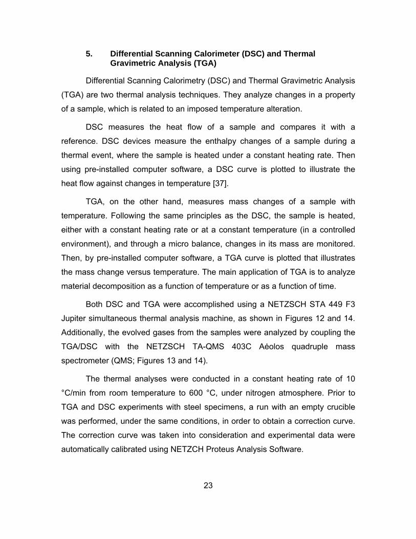
Figure 23. Image of a “collapsed” hump on the surface of a 5 min, 2.5 V, at 90 °C anodized steel in 50 wt% NaOH solution

Due to the highly corroded appearance of the anodized surface resulting

from the NaOH solution anodizations and the variations in their oxide

morphology, an alternative electrolyte, the 0.50 wt% NH4F, 3 wt% DI water in EG

solution, was examined. Anodizations were performed at a range of 10 to 50 V

and the results showed the creation of a severely pitted oxide surface (Figure

24). This large amount of holes in the anodized surface of steel is due to the high

water concentration on the solution and the creation of bubbles as the surface of

the sample is subjected to the electrochemical anodization. The creation of

bubbles and subsequently of holes in the surface is promoted when high

potentials are used. Furthermore, anodization duration was kept to 5 min since

any attempt made to increase it resulted in a heavily corroded topography (as

displayed in Figure 25).

38

Figure 24. SEM images showing the pitting effect on the surface of anodized HY-80 steel under potentials of (a) 10 V,(b) 25 V, (c) 30

V, and (d) 50 V

Figure 25. SEM image of steel surface under 10 min, 50 V anodization in 0.50 wt% NH4F, 3 wt% DI water EG solution at 60 °C

39

In low potential anodizations, the main structures appearing are 20 nm

pores and nano channel like complexes that develop on round patterns (Figure

26). By further increasing the potential, the same two structures continue to

appear until 50 V are applied. Above this potential, the topography seems to

collapse and the final product shows signs of an amorphous oxide layer (Figure

29). By repeating the experiments at lower temperatures (50 °C), it becomes

clear that the construction of nanoporous pits is favored over nano channeling

patterns, but the final morphology still remains highly heterogeneous.

Figure 26. SEM images of anodized sample in 10 V, 60 °C, 0.50 wt% NH4F, 3 wt% DI water in EG electrolyte under (a) low, (b)

medium, and (c) high magnification

40

Figure 27. SEM images of anodized sample in 25 V, 60 °C, 0.50 wt% NH4F, 3 wt% DI water in EG electrolyte under (a) low and (b) high

magnification

Figure 28. SEM images of anodized sample in 40 V, 60 °C, 0.50 wt% NH4F, 3 wt% DI water in EG electrolyte focusing on (a) nano

porous and (b) nano channeling structure

41

Figure 29. SEM macroscopic images of anodized sample in 50 V, 60 °C, 0.50 wt% NH4F, 3 wt% DI water in EG electrolyte

In an effort to avoid the extreme surface pitting due to the high

concentration of water in the previous electrolyte, a new solution was used with

less concentration in NH4F and water. The experiments on 0.37 wt% NH4F, 1.8

wt% DI water EG solution proved that a nanoporous oxide layer is produced with

this electrolyte, as seen in Figures 30 and 31, between the range of 20 to 30 V.

Initially 20 nm diameter pits were developed on the surface of the steel, which

coalesced together to form larger pores as anodization continued. This progress

of the oxide layer is relatively slow in low potential anodizations compared to the

one appearing in applied potential of 40 V or more. As a result of it, when

conducting anodizations under a voltage of 20 V, the average diameter of the

constructed pores was 150 nm, whereas for 30 V, the resulted pores were of

approximately 120 nm diameters. In even higher voltages, though, the evolution

of the oxide happens so fast that it totally consumes the initially developed

topography, as Figures 32 and 33 indicate.

42

Figure 30. SEM images on high (left) and low (right) magnification of nanoporous structure under 1 h anodization in a 0.37 wt% NH4F,

1.8 wt% DI water EG solution on 20 V at 25 °C



43





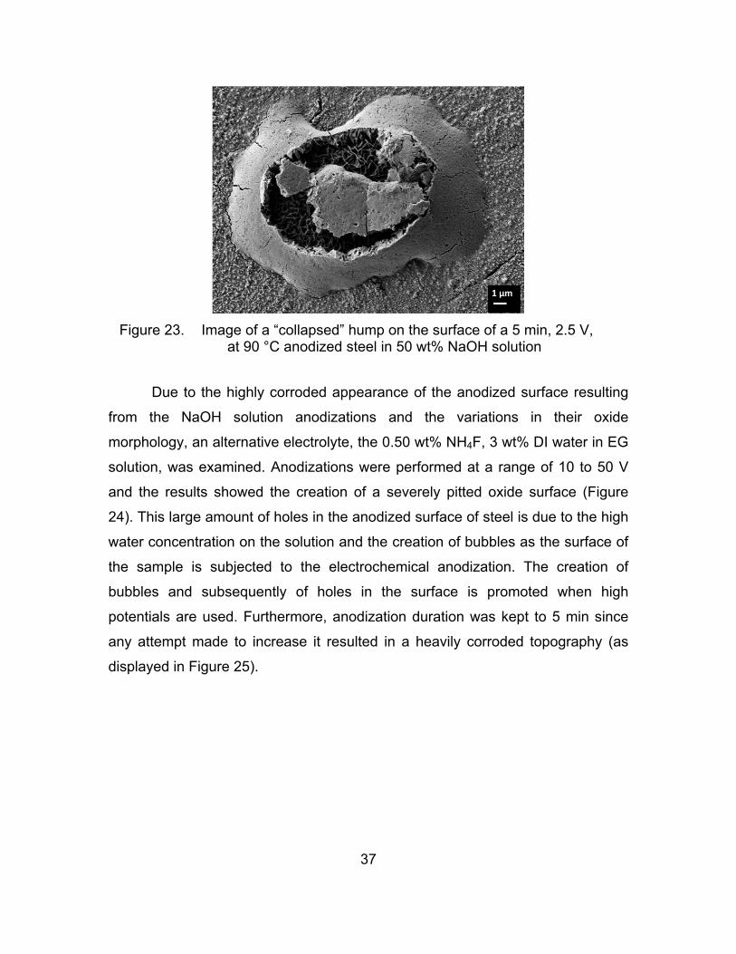
By further decreasing the amount of water contained in the electrolyte and

by changing the anodization approach from potentiostatic to galvanostatic, it was

possible to achieve uniform distribution of nanoporous oxide morphologies. The

secondary electron images in Figures 34 and 35 indicate a self-oriented

nanoporous anodic film created with current densities between 30 and 85 A/m2.

Cylindrical nanopores of 20 nm average diameter were initially developed and

merged together to form larger pores whose diameter was measured to be

44

approximately 90 nm regardless of the current density in the anodizing range

used.

A thorough SEM examination revealed very closely spaced porous

structures along the scratches (polishing lines) on these surfaces, and a similar

structure is observed along grain boundaries as well in Figure 37.

Figure 34. SEM images of nanoporous structure under 5 min (left) or 15 min (right) anodization in a 0.37 wt% NH4F, 0.9 wt% DI water EG

solution with applied current density of 30A/m2 at 25 °C

Figure 35. SEM images of nanoporous structure under 5 min (left) or 15 min (right) anodization in a 0.37 wt% NH4F, 0.9 wt% DI water EG

solution with applied current density of 45A/m2 at 25 °C

45

Figure 36. SEM images of nanoporous structure under 5 min anodization in a 0.37 wt% NH4F, 0.9 wt% DI water EG solution with applied

current density of 85A/m2 at 25 °C

Figure 37. SEM image on a 5 min anodized surface under 85A/m2

Finally, further examination revealed that by increasing the anodization

time, the growth of the homogeneous nanoporous pattern is replaced with large

regions of oxide growing over the previous nanoporous layer. This is a procedure

similar to the one described in the 1.8wt% solutions that evolves rapidly under

higher applied currents (Figure 38).

46

Figure 38. SEM images on a lower magnification of samples anodized for 15 min at 60 A/m2 (top) and 85A/m2 (bottom)

The morphological features of the anodized surfaces studied here can be summarized as follows:

Anodization in NaOH solutions creates heterogeneous and highly corroded surfaces. The surface oxide consists of mainly three morphologies: the hexagonal and spherical patterns, which appear on the outside layer of the surface, and the nanoporous channels, which are formed on the steel substrate.

In EG solutions of 0.50 wt% NH4F, 3 wt% DI water, a severely pitted surface was obtained. In the voltage range of 10–40 V, two main morphologies appear: 20 nm porous topographies and nano channel like complexes that develop on cyclical patterns. However,

47

for potentials greater than 50 V, the surface shows signs of an amorphous oxide layer.

Anodizations in EG solutions of 0.37 wt% NH4F, 1.8 wt% DI water between 20–30 V create a homogeneous nanoporous oxide layer with an average pore diameter varying from 120 to 150 nm depending on the anodization voltage. Nevertheless, when the anodization potential increases more than 40 V, the oxide will grow and consume the previous layer

While in EG solutions of 0.37 wt% NH4F, 0.9 wt% DI water, galvanostatic anodization self-oriented nanoporous anodic film with an average porous diameter of 90 nm are produced only between current densities from 30 to 85 A/m2. Moreover, when anodization time exceeds 15 min, the oxide grows over the previous nanoporous layer.

B. GROWTH KINETICS OF NANOPOROUS ANODIC FILMS

SEM analysis showed that homogeneous nanoporous structures can be

formed on HY-80 steels in an EG containing ammonium fluoride and water

electrolyte under both potentiostatic and galvanostatic anodization. In order to

study the kinetics over the creation and growth of this nanoporous structure, the

current density and the potential were constantly monitored and plotted.

In case of potentiostatic anodization, a typical current densities versus

time graph obtained is plotted in Figure 39. There are many similarities between

the current density transient obtained with the one observed in the anodization of

iron [25], which can be described in the following three stages. In order to clearly

see the three stages, three plots with appropriate axes scales for the same set of

data were shown in this figure.

48

Figure 39. Current density versus time curve recorded during anodization in 0.37 wt% NH4F, 1.8 wt% DI water EG solution at 25 °C during

various time intervals

0

0.05

0.1

0.15

0.2

0.25

0.3

0.35

0.4

0.45

0 5 10 15 20 25 30 35 40 45 50 55

Current Density in

A/m

m²

tim in sec

30 volts

40 Volts

50 Volts

0

0.05

0.1

0.15

0.2

0.25

0.3

0.35

0.4

0.45

0 100 200 300 400 500

Current Density in

A/m

m²

tim in sec

30 volts

40 Volts

50 Volts

0

0.1

0.2

0.3

0.4

0.5

0.6

0.7

0.8

0.9

0 600 1200 1800 2400 3000

Current Density in

A/m

m²

tim in sec

30 volts

40 Volts

50 Volts

49

At the first stage, current density decreases rapidly within 20 seconds.

This drop is because of the fast growth of an oxide layer on a steel plate in an

EG solution containing fluorides and water, which via the overall chemical

reaction of equation (8), subsequently leads to a resistance increase. At this

point, the initial 20 nm diameter pits are formed on the oxide surface, which with

time gradually merge into larger pores due to the following chemical dissolution

of the oxide.

32 3 6 212 6 2 3Fe O F H FeF H O (8)

At the second stage, a slow increase of current density is observed, which

relates to the decreased surface resistance of the oxide layer via gradual

formation of the metal-fluoride complex anion according to equation (8).

Finally, in the third stage, the current density reaches a constant value,

which implies that a dynamic equilibrium between the rate of oxide formation and

that of the oxide dissolution has been achieved.

The observed electrochemical evolution was explained in the model

proposed by Xie et al. [25] of the formation of iron oxide nanotubes in Fe foils.

When anodization begins, subsequent to the formation of an oxide layer, fine pits

are formed due to the localized dissolution of the oxide layers by F- ion. Due to

the barrier level being thin at the bottom of the pore while the electric field

intensity across the remaining barrier layer is high, the pore becomes wider and

deeper. The presence of substantial amounts of H+ in solution greatly enhances

the dissolution process and thus the fine pore coalescence and growth. As the

larger pores become deeper and deeper, a highly oriented nanoporous structure

is established.

In the case of 50 V applied voltage, an anomaly to the previous described

curve is reported. After the initial rapid drop in current density, a constant

increase is observed for 45 min followed by a decrease in current density. The

explanation behind this phenomenon is that because of the high potential, a

50

dynamic equilibrium between oxide growth and dissolution is never established

and the dissolution process is favored over the oxide formation.

To study the electrochemical behavior of the anodic film during the

formation of the iron-oxide nanoporous structure in galvanostatic anodization, the

potential densities versus time graphs were plotted, as seen in Figures 40 and

41. Since the oxide creation and growth are similar to the process described

above, similar behavior is obtained. Again, after the initiation of oxidation, the fast

growth of the oxide leads to resistance increase, which subsequently causes the

potential to increase almost linearly. The fine pits are making their appearance

and they merge together through chemical dissolution forming larger pores as

equation (8) implies. As the pores deepen, the thickness of the barrier layer

decreases, and the voltage needed for driving the same current decreases

accordingly. After a period of adjustment, a steady state formation voltage is

obtained. This stage lasts from one to three minutes depending on the

anodization current density applied, where the samples under higher current

densities reach the equilibrium condition sooner. For particular values of applied

densities (such as 45 A/m2 or lower), the rates of oxidation and dissolution can

balance each other exactly right after the voltage increase and a steady state can

eventually be reached with barrier layer thickness and voltage remaining

constant with time thereafter [45].

51

Figure 40. Potential density versus time curve recorded during 5 min anodization in 0.37 wt% NH4F, 0.9 wt% DI water EG solution at

25 °C

Figure 41. Potential density versus time curve recorded during 15 min anodization in 0.37 wt% NH4F, 0.9 wt% DI water EG solution at

25 °C

C. CHARACTERIZATION WITH EDS

Initially EDS was used in an effort to identify the difference between the

two main structures appearing on the surface of anodized steels in NaOH

solutions. EDS analysis revealed that the spherical structured oxide included

0

50

100

150

200

250

300

350

400

010

20

30

40

50

60

70

80

90

100

110

120

130

140

150

160

170

180

190

200

210

220

230

240

250

260

270

280

290

Potential in

mV/m

m²

Time in sec

30 A/m²

45 A/m²

50 A/m²

85 A/m²

0

50

100

150

200

250

300

350

400

0

60

120

180

240

300

360

420

480

540

600

660

720

780

840

Volatege

in m

V/m

²

time in sec

45

85

52

larger amounts of oxygen than the hexagonal crystal shaped oxides, as indicated

in Figures 42 and 43 and Tables 7 and 8. In spite of the fact that EDS is a useful

method to identify the chemical composition of a specimen, in this particular case

the relatively small thickness of the constructed oxide layer affected the

measurements as the electron interaction volume contained the surface oxide as

well as the underlying alloy. The characteristic X-rays from the substrate layer of

HY-80 interfered with those that were emitted from the surface and, as a result,

Fe appeared to be the predominant element, even in structures where the ratio

between oxygen and iron atoms was expected to be different.

Figure 42. EDS spectrum from the spherical structure oxide on anodized steel surface after 5 min in a 50 wt% NaOH solution with applied

voltage of 2.5 V at 75 °C

Table 7. EDS quantitative analysis showing weight and atomic number percent of elements in anodized steel area of Figure 42

Element Wt% At% Oxygen (O) 13.38 35.02 Iron (Fe) 86.62 64.98 Matrix Correction ZAF

53

Figure 43. EDS spectrum from the hexagonal structure oxide on anodized steel surface after 5 min in a 50 wt% NaOH solution

with applied voltage of 2.5 V at 75 °C

Table 8. EDS quantitative analysis showing weight and atomic number percent of elements in anodized steel area of Figure 43


EDS characterization proved to be inconclusive also in the case of

anodized steels in 0.37 wt% NH4F EG with the constructed oxide appearing to

consist of Fe from 80% to 90%, as shown in Figures 44 and 45 and Tables 9 and

10.

54

Figure 44. EDS spectra from anodized steel after 1 hour in a 0.37 wt% NH4F, 1.8 wt% DI water EG solution with applied voltage of 20 V

at room temperature

Table 9. EDS quantitative analysis showing weight and atomic number percent of elements in the Figure 44 anodized steel


Figure 45. EDS spectra from anodized steel after 5 min in a 0.37 wt% NH4F, 0.9 wt% DI water EG solution with applied current density

of 40A/m2 at room temperature

55

Table 10. EDS quantitative analysis showing weight and atomic number percent of elements in the Figure 45 anodized steel


D. CHARACTERIZATION WITH XRD

X-ray diffractometry was used in every sample to investigate the type of

surface oxides formed during anodization and the effects that the annealing

process had on them. The following figures show the X-ray diffraction patterns of

the anodized iron oxides for different treatments.

XRD patterns from samples anodized in NaOH solutions showed peaks

corresponding to martensitic steel, wustite, Fe0.93O, and magnetite, Fe3O4. As the

applied voltage, anodization time, or temperature increased, so did the fraction of

magnetite. However, after the annealing process, magnetite peaks reduced their

intensity (nearly disappeared), suggesting that all magnetite is converted to

wustite, as can be seen in Figures 46 and 47.

In case of anodization in EG solutions of 0.50 wt% NH4F, 3 wt% DI water,

the only XRD peaks appearing are of martensitic steel and wustite, Fe0.93O. After

annealing the oxide, Fe0.93O is converted into Fe2O3. In low voltage anodizations

(such as the 30 V anodization appearing in Figure 48), the structure of the oxide

is maghemite, which has a cubic crystal structure. As the anodization voltage

increases, the phase is hematite, Fe2O3, with a trigonal hexagonal structure

(XRD is shown in Figure 49 after 50 V anodization).

In the 0.37 wt% NH4F, 1.8 wt% DI water EG solutions, again before

annealing, only XRD peaks for martensitic steel and wustite are visible; however,

after heat treatment, a very small amount of magnetite is also observed as a

secondary phase, and the experiments conducted between applied voltages of

20 V and 50 V did not show any significant change in the constructed oxide

(Figure 50).

56

Finally, in the case of the 5 min galvanostatic anodization in 0.37 wt%

NH4F, 0.9 wt% DI water EG solutions, even after annealing, the only peaks

observed belong to wustite (Fe0.93O) and to martensitic steel. Furthermore, by

changing the anodization parameters of the applied current density within a

range of 30 to 85 A/m2 and of the anodization time from 5 to 15 min, the oxide

layer structure remains unaffected (Figure 51).

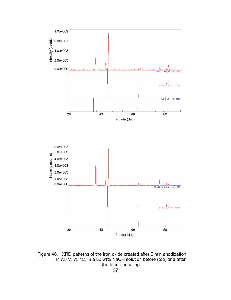
57

Figure 46. XRD patterns of the iron oxide created after 5 min anodization in 7.5 V, 75 °C, in a 50 wt% NaOH solution before (top) and after

(bottom) annealing

Inte

nsity

(co

unt

s)

0.0e+000

2.0e+003

4.0e+003

6.0e+003

8.0e+003

C0.055 Fe1.945, 00-044-1290

Fe0.93 O, 04-011-7344

2-theta (deg)

20 40 60 80

Fe3 O4, 03-065-3107

Inte

nsity

(co

unt

s)

0.0e+000

1.0e+003

2.0e+003

3.0e+003

4.0e+003

5.0e+003

6.0e+003

C0.055 Fe1.945, 00-044-1290

2-theta (deg)

20 40 60 80

Fe0.93 O, 04-011-7344

58

Figure 47. XRD patterns of the iron oxide created after 5 min anodization in 12.5 V, 75 °C, in a 50 wt% NaOH solution before (top) and after

(bottom) annealing

Inte

nsity

(co

unt

s)

0

1000

2000

3000

4000

C0.055 Fe1.945, 00-044-1290

Fe3 O4, 03-065-3107

2-theta (deg)

20 40 60 80

Fe0.93 O, 04-011-7344

Inte

nsity

(co

unt

s)

0.0e+000

1.0e+003

2.0e+003

3.0e+003

4.0e+003

5.0e+003

6.0e+003

C0.055 Fe1.945, 00-044-1290

Fe0.93 O, 04-011-7344

2-theta (deg)

20 40 60 80

Fe3 O4, 03-065-3107

59

Figure 48. XRD patterns of the iron oxide created after 5 min anodization in 30 V, 50 °C, in a 0.50 wt% NH4F, 3 wt% DI water EG solution

before (top) and after (bottom) annealing

Inte

nsity

(co

unt

s)

0.0e+000

2.0e+003

4.0e+003

6.0e+003

8.0e+003

1.0e+004

1.2e+004

C0.055 Fe1.945, 00-044-1290

2-theta (deg)

20 40 60 80

Fe0.93 O, 04-011-7344

Inte

nsity

(co

unt

s)

0.0e+000

2.0e+003

4.0e+003

6.0e+003

C0.055 Fe1.945, 00-044-1290

Fe0.93 O, 04-011-7344

2-theta (deg)

20 40 60 80

Fe2 O3, 04-016-4345

60

Figure 49. XRD patterns of the iron oxide created after 5 min anodization in 50 V, 50 °C, in a 0.50 wt% NH4F, 3 wt% DI water EG solution

before (top) and after (bottom) annealing

Inte

nsity

(co

unt

s)

0.0e+000

5.0e+003

1.0e+004

Fe0.93 O, 04-011-7344

2-theta (deg)

20 40 60 80

C0.055 Fe1.945, 00-044-1290

Inte

nsity

(co

unts

)

0.0e+000

2.0e+003

4.0e+003

6.0e+003

8.0e+003

C0.055 Fe1.945, 00-044-1290

2-theta (deg)

20 40 60 80

Fe2 O3, 04-016-5466

61

Figure 50. XRD patterns of the iron oxide created after 60 min anodization in 30 V, 25 °C, in a 0.37 wt% NH4F, 1.8 wt% DI water

EG solution before (top) and after (bottom) annealing

Inte

nsity

(co

un

ts)

0.0e+000

2.0e+003

4.0e+003

6.0e+003

8.0e+003

1.0e+004

Fe0.93 O, 04-011-7344

2-theta (deg)

20 40 60 80

C0.055 Fe1.945, 00-044-1290

Inte

nsity

(co

unts

)

0.0e+000

2.0e+003

4.0e+003

6.0e+003

8.0e+003

Fe0.93 O, 04-011-7344

C0.055 Fe1.945, 00-044-1290

2-theta (deg)

20 40 60 80

Fe3 O4, 03-065-3107

62

Figure 51. XRD patterns of the iron oxide created after 15 min anodization in 45A/m2, 25 °C, in a 0.37 wt% NH4F, 0.9 wt% DI

water EG solution before (top) and after (bottom) annealing

Inte

nsity

(co

unt

s)

0.0e+000

2.0e+003

4.0e+003

6.0e+003

8.0e+003

1.0e+004

Fe0.93 O, 04-011-7344

2-theta (deg)

20 40 60 80

C0.055 Fe1.945, 00-044-1290

Inte

nsity

(co

unt

s)

0.0e+000

2.0e+003

4.0e+003

6.0e+003

8.0e+003

C0.055 Fe1.945, 00-044-1290

2-theta (deg)

20 40 60 80

Fe0.93 O, 04-011-7344

63

Summarizing the results of XRD, it is observed that

Anodization in NaOH solutions is capable of producing magnetite with optimum conditions being the applied voltages of 12.5 V under elevated temperatures of 90 °C. The applied annealing process, however, did not have satisfactory results.

In EG solutions of 0.50 wt% NH4F, 3 wt% DI water, the oxide that is finally obtained is hematite under an applied voltage of 50 V at a temperature of 50 °C.

In EG solutions of 0.37 wt% NH4F, 1.8 wt% DI water, the finally obtained oxides are wustite (Fe0.93O) with magnetite as a secondary phase.

However, in the galvanostatic anodization, only Fe0.93O oxide is present.

E. CHARACTERIZATION WITH FIB

Based on the observed morphology of HY-80 steel samples anodized in

various conditions, highly ordered iron oxide nanopores are formed during

galvanostatic anodization in EG solutions containing 0.37 wt% NH4F and 0.9 wt%

DI water. FIB milling was carried out on samples that have been anodized under

these conditions to observe the cross sectional features of the oxide film.

Specifically the oxide layer growth on the surface of steel samples anodized

under constant current density of 45 A/m2 was studied.

The thickness of the oxide layer was measured by using FIB to create a

transverse incision on the surface of the specimen, allowing SEM to examine its

morphology and take the pictures that appear in Figures 52 and 53. The obtained

oxide layer after a 5 min anodization is quite thin, with thickness varying between

490 to 140 nm. However, by increasing the anodization time, thickness also

increases, and in a 15 min anodization, a layer of 290 to 650 nm thickness was

observed.

The width of the walls of columns around pores was also calculated. In the

5 min anodization, the column surrounding each pore had an average width of 55

nm, but as the layer grew, so did the width of the walls, and after 15 min of

anodizing, it reached an average width of 66 nm.

64

Figure 52. FIB image of anodized steel surface under current density of 40 A/m2 in EG solution of 0.37 wt% NH4F, 0.9 wt% DI water

concentration, for 5 min

Figure 53. FIB image of anodized steel surface under current density of 45 A/m2 in EG solution of 0.37 wt% NH4F, 0.9 wt% DI water

concentration, for 15 min

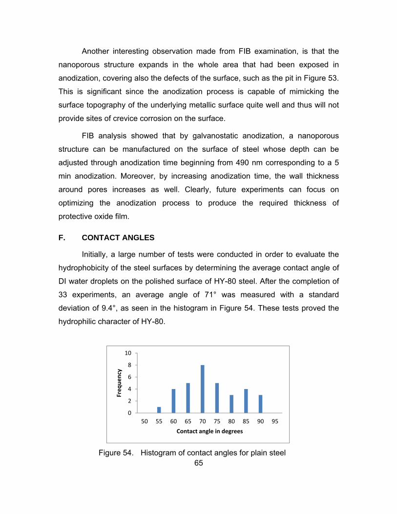
65

Another interesting observation made from FIB examination, is that the

nanoporous structure expands in the whole area that had been exposed in

anodization, covering also the defects of the surface, such as the pit in Figure 53.

This is significant since the anodization process is capable of mimicking the

surface topography of the underlying metallic surface quite well and thus will not

provide sites of crevice corrosion on the surface.

FIB analysis showed that by galvanostatic anodization, a nanoporous

structure can be manufactured on the surface of steel whose depth can be

adjusted through anodization time beginning from 490 nm corresponding to a 5

min anodization. Moreover, by increasing anodization time, the wall thickness

around pores increases as well. Clearly, future experiments can focus on

optimizing the anodization process to produce the required thickness of

protective oxide film.

F. CONTACT ANGLES

Initially, a large number of tests were conducted in order to evaluate the

hydrophobicity of the steel surfaces by determining the average contact angle of

DI water droplets on the polished surface of HY-80 steel. After the completion of

33 experiments, an average angle of 71° was measured with a standard

deviation of 9.4°, as seen in the histogram in Figure 54. These tests proved the

hydrophilic character of HY-80.

Figure 54. Histogram of contact angles for plain steel

0

2

4

6

8

10

50 55 60 65 70 75 80 85 90 95

Frequency

Contact angle in degrees

66

The anodized surface showed a change in its wettability properties from

slightly hydrophilic to hydrophobic behavior. In each anodization method applied,

the behavior of the steel remained hydrophobic. Photographs in Figure 55 show

a comparison of the appearance of the water drops on various surfaces as

indicated. The measured data are summarized in Tables 11 and 12. The best

results, however, were obtained using anodization in a NaOH solution. The

anodized samples showed contact angles varying in a range of 131° to 146°. The

largest contact angles were reported when applying a voltage of 12.5 V in an

electrolytic temperature of 90 °C for a period of time between 3 min (146°) and

10 min (145°).

When EG-based electrolyte was used, the produced surfaces were slightly

less hydrophobic, with contact angles varying between 110° and 138°. The

surfaces manufactured with this method decreased in wettability as the

concentration of NH4F in the solution increased. Therefore, the greatest contact

angles were observed when anodizations took place in 0.50 wt% NH4F solutions,

and particularly under voltage of 50 V, at 60 °C for a duration of 5 min, a contact

angle of 138° appeared, which was the maximum obtained for this solution. The

surfaces created in 0.37 wt% NH4F electrolyte appear to have similar wetting

properties. In the case of potentiostatic anodization in 1.8 wt% DI water

concentration, the maximum contact angle was 118° and appeared after

anodizing under voltage of 30 V for 1 hour, while in the case of galvanostatic

anodization under a constant current density of 82 A/m² at room temperature for

15 min, a 126° angled was achieved.

Table 11. Contact angles of DI water on the surface of anodized steel under NaOH electrolyte

Anodization condition 7.5 V 12.5 V 75 °C – 5 min 134° 136°

90 °C – 3 min 146°

90 °C – 5 min 131° 90 °C – 10 min 145°

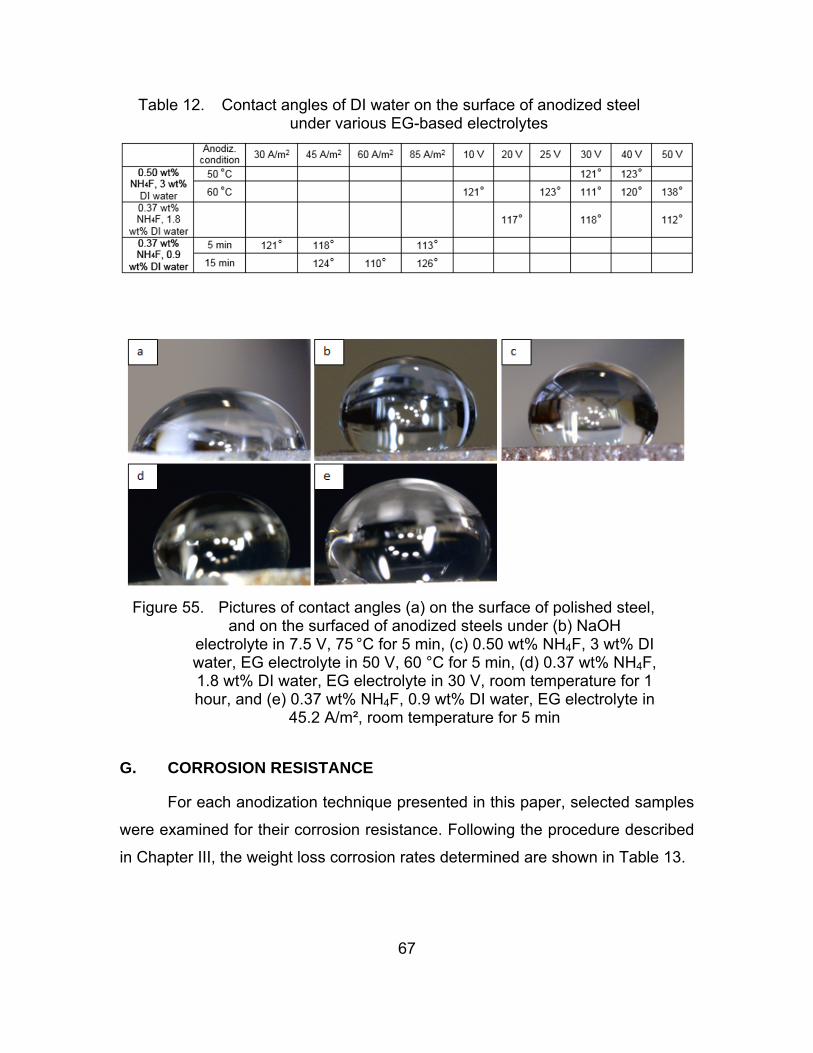
67

Table 12. Contact angles of DI water on the surface of anodized steel under various EG-based electrolytes

Figure 55. Pictures of contact angles (a) on the surface of polished steel, and on the surfaced of anodized steels under (b) NaOH

electrolyte in 7.5 V, 75 °C for 5 min, (c) 0.50 wt% NH4F, 3 wt% DI water, EG electrolyte in 50 V, 60 °C for 5 min, (d) 0.37 wt% NH4F, 1.8 wt% DI water, EG electrolyte in 30 V, room temperature for 1 hour, and (e) 0.37 wt% NH4F, 0.9 wt% DI water, EG electrolyte in

45.2 A/m², room temperature for 5 min

G. CORROSION RESISTANCE

For each anodization technique presented in this paper, selected samples

were examined for their corrosion resistance. Following the procedure described

in Chapter III, the weight loss corrosion rates determined are shown in Table 13.

68

Table 13. Corrosion rates for HY-80

Mass loss (mg/mm²)

MPY mm/yr

corrosion in seawater polished steel 0.030 4.955 0.1258 anodized in NaOH solution

0.031 5.083 0.1291

anodized in 0.50 wt% NH4F, 3 wt% DI water, EG solution

0.044 7.387 0.1876

anodized in 0.37 wt% NH4F, 1.8 wt% DI water, EG solution

0.028 4.600 0.1168

anodized in 0.37 wt% NH4F, 0.9 wt% DI water, EG solution

0.029 4.759 0.1209

corrosion in salt water polished steel 0.032 5.355 0.1360 anodized in NaOH solution

0.051 8.518 0.2164

anodized in 0.50 wt% NH4F, 3 wt% DI water, EG solution

0.078 12.967 0.3294

As can be deduced from Table 13, the corrosion in seawater was less

than the corrosion experienced in 3.5wt % NaCl solution. Moreover, not all of the

anodized surfaces displayed improved anticorrosive properties. Especially

anodization under 0.50 wt% NH4F, 3 wt% DI water, the EG solution worsened

the corrosive properties of the steel by far, while in the case of anodization under

a NaOH solution, the corrosion rates increased but at a lesser grade.

However, the self-oriented nanoporous structures created on anodized

samples under EG-based solutions of 0.37 wt% NH4F concentration granted HY-

80 steel corrosion protection. Specifically, the corrosion rate of steel dropped

from 5 MPY to a range between 4.6 to 4.8 MPY.

69

H. BIOFOULING

1. Thermal Analysis

Preliminary thermal analysis was conducted on selected HY-80

specimens in order to verify the capability of these techniques to detect organic

material depositions on the surface of steel. During those examinations, the main

focus was the identification of carbon traces, which are indicative of the presence

of living organisms such as bacteria and micro-organisms. For this reason, four

different samples were prepared in the following conditions:

1. polished steel 2. polished steel with the addition of mold 3. polished steel left to corrode inside stagnant natural water for one

week 4. polished steel left to corrode inside 3.5 wt% NaCl solution for one

week

Each of these samples was analyzed with TGA, DSC, and QMS

techniques; the aggregate results can be seen in Figures 56, 57, and 58.

70

Figure 56. TGA analysis

[1] Steel exposed in salt water [2] Steel exposed in seawater [3] Steel with mold [4] Plain steel

71

Figure 57. DSC analysis

[1] Steel exposed in salt water [2] Steel exposed in seawater [3] Steel with mold [4] Plain steel

72

Note. The noticeable red dotted line shows the emission of CO2 gases at 470 °C on the steel specimen with the mold.

Figure 58. TGA/QMS diagram

As expected, the DSC curve of the sample with mold presented a

distinguish slope as a result of an exothermic reaction at 470 °C, which was later

examined through QMS and found to be carbon combustion and the creation of

CO2 gases. Moreover, both the untreated steel and that corroded in 3.5wt%

NaCl-DI water solution samples exhibited similar curves that did not display any

slope due to carbon combustion and, furthermore, no emission of CO2 gases

was recorded. In the test involving the steel sample that was exposed in

seawater, again no traces of carbon were found. The last experiment was then

repeated with another HY-80 steel sample corroded under the same conditions

as the previous, trying to verify the results, but again the analysis produced

similar data.

[1] Steel exposed in salt water TG [2] Steel exposed in seawater TG [3] Steel with mold TG [4] Plain steel TG [5] Steel exposed in salt water Ion Current [6] Steel exposed in seawater Ion Current [7] Steel with mold Ion Current [8] Plain steel Ion Current

73

Therefore, the conclusion can be made that either there was no micro-

organism attachment onto the surface of the sea-corroded samples, or the

thermal methods could not identify it, presumably due to the extremely low

concentrations of bio organisms present in the small quantity of seawater used in

these experiments. The fact that the behavior in the natural seawater (which may

have some organic species present in it) was identical to that of the 3.5wt% NaCl

-DI water solution, which most likely did not have any biofilm-producing matter in

it, supports this speculation. Anyway, the use of the thermal method analysis to

assess the content of biofouling on the surface requires an examination with

more controlled experiments with controlled amounts of microorganisms

introduced in the corrosive solutions; other characterization methods should also

be investigated.

2. SEM/EDS Analysis

Following the inconclusive nature of the TGA studies, SEM and EDS

examinations were performed in order to verify the existence of living

microorganisms on the surface of steel left in seawater over a period of 10 days.

In order to compare the features formed on the steel surface exposed to marine

conditions, both natural Monterey seawater and a 3.5wt%NaCl in DI water

solution were examined since the latter solution does not contain any significant

amount of microorganisms present in it. Figure 59 shows a secondary electron

image showing the typical appearance of the corrosion product formed in the DI

water–3.5wt%NaCl solution, and the EDS analysis confirmed the presence of

mostly Fe and O.

SEM images of steel plates that had been left in natural seawater revealed

not only the usual characteristic presence of iron oxides and rust, but also

several distinct features with dimensions varying from 9 µm to 81 µm, as

depicted in Figures 60 and 61. This observation has led to the deduction that the

appearance of these features is something exclusively associated with the

contents of ocean water.

74

EDS analysis on these morphologies revealed the elemental composition

of these crystals to be rich in carbon as well as calcium, magnesium, and

oxygen, as seen in Figure 63 and Table 16. However, the EDS analysis for

oxygen that is shown is not accurate due to the high errors associated with low

atomic number elements in this technique. In spite of the increased content of

organic compounds, the observed shapes do not correspond to living

microorganisms, but have been identified as calcium carbonate (CaCO3) crystals,

which are known to grow on steel surfaces. The presence of Ca2+ and Mg2+ in

seawater creates a cathodic reduction of oxygen under the following equations

which precipitate in CaCO3 and Mg(OH)2 [46]:

23 2 3Ca HCO OH H O CaCO (9)

222 ( )Mg OH Mg OH (10)

The resulting CaCO3 crystals can appear in many crystalline forms, as

illustrated in Figure 64. The optical resemblance with the obtained carbon-

enhanced shapes on the surface of HY-80 plates is obvious; therefore, they are

identified as calcites and aragonites (crystalline forms of calcium carbonate).

Extensive SEM/EDS examination did not show any traces of bacteria or other

microorganisms. This could be due to the low content of microorganisms in the

ocean water used in the experiments, thus further investigation should be done

with microbiological techniques such as bacteria cultivation and colonization.

These microscopy results are in agreement with the TGA results that showed no

measurable carbon decomposition during thermal exposure of the seawater-

corroded samples.

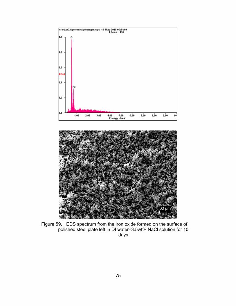
75

Figure 59. EDS spectrum from the iron oxide formed on the surface of polished steel plate left in DI water–3.5wt% NaCl solution for 10

days

76

Table 14. EDS quantitative analysis showing weight and atomic number percent of elements of iron oxide appearing in Figure 59


Figure 60. SEM images of calcium carbonate (CaCO3) crystals with their corresponding dimensions appearing in red lines

77

Figure 61. SEM images of aragonite crystal in low (left) and high (right) magnification

Figure 62. EDS spectrum from a calcium carbonate (CaCO3) crystal

78

Figure 63, continued on next page

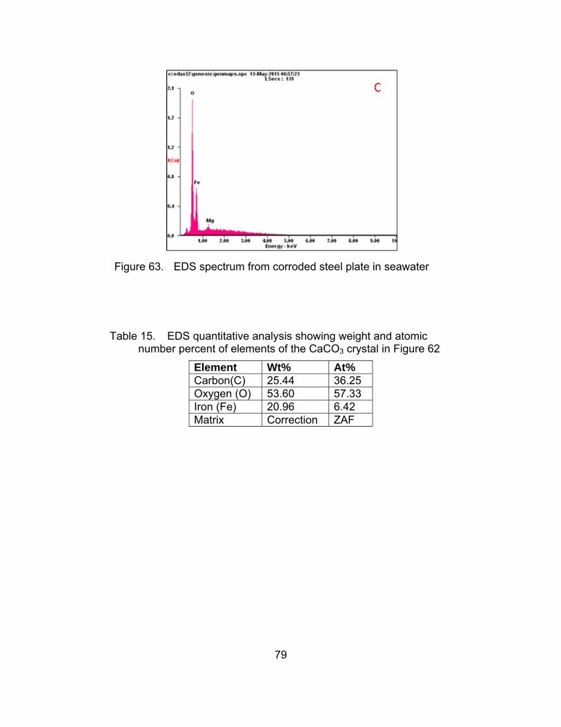
79

Figure 63. EDS spectrum from corroded steel plate in seawater

Table 15. EDS quantitative analysis showing weight and atomic number percent of elements of the CaCO3 crystal in Figure 62

Element Wt% At% Carbon(C) 25.44 36.25 Oxygen (O) 53.60 57.33 Iron (Fe) 20.96 6.42 Matrix Correction ZAF

80

Table 16. EDS quantitative analysis showing weight and atomic number percent of elements appearing in the corroded steel

surface of Figure 63

Area A Element Wt% At% Carbon (C) 30.12 36.47 Oxygen (O) 69.88 63.53 Matrix Correction ZAF

Area B

Element Wt% At% Carbon (C) 03.00 07.27 Oxygen (O) 27.18 49.41 Iron (Fe) 59.53 31.01 Magnesium (Mg) 10.29 12.32 Matrix Correction ZAF

Area C

Element Wt% At% Oxygen (O) 28.65 57.54 Iron (Fe) 69.48 39.98 Magnesium (Mg) 01.87 02.48 Matrix Correction ZAF

81

Figure 64. SEM images of various crystalline forms of CaCO3 crystals such as calcite in (a) and aragonite in (b) and (c), from [46]

82


83

VI. CONCLUSIONS

This study shows that homogenous nanoporous anodic films can be

formed on HY-80 steels in an EG solution containing ammonium fluoride and

water electrolyte. However, the increased concentration of water in combination

with elevated temperatures resulted in the severe pitting of the surface of the

anodized specimen and in the creation of nano channeling patterns that affected

the uniformity of the surface oxide layer. Nevertheless, by decreasing

anodization temperature and water concentration, homogenous nanoporous

oxide layers were successfully produced by the following two methods.

Through potentiostatic anodization in a range between 20 to 30 V in a

0.37 wt% NH4F, 1.8 wt% DI water EG solution at room temperature,

homogenous nanoporous anodic films were produced. However, the optimum

anodization conditions are under 30 V for 1 hour with a solution maintained at

approximately 25 °C, which creates an oxide layer with a 120 nm average pore

diameter. Furthermore, by annealing the sample at 400 °C for 2 hours, it

transforms into wustite (Fe0.93O) and magnetite. The produced surface exhibits

decreased wettability, with a water contact angle of approximately 118°, which is

an improvement in the wetting properties of polished HY-80 by 166%. It also

reduced the corrosion rate of HY-80 steel by approximately 7.2%.

The second successful technique of constructing a highly oriented

nanoporous oxide is through galvanostatic anodization in a current density range

between 30 and 85 A/m2 in 0.37 wt% NH4F, 0.9 wt% DI water EG solution at

room temperature. In this method, the optimum anodizing condition is under 45

A/m2 on an approximately 25 °C solution for 15 min. This results in the formation

of a 290 nm to 650 nm thick oxide with an average 66 nm distance between each

pore. The crystal structure of the oxide is that of wustite (Fe0.93O) and through the

annealing process, its structure remained unaffected. Again, in this case, the

surface oxide topography granted the steel exceptional hydrophobic behavior

84

(124°) with water contact angles 177% greater than those of the untreated HY-80

steel and slightly improved (by 4%) its corrosion properties.

Concluding this study, antifouling properties of the constructed

morphologies were examined with the use of both thermal (TGA/DSC) and

SEM/EDS quantitative analysis. However, they did not show microorganism

attachments during exposure on stagnant natural water, thus antifouling

properties need to be examined through experiments with controlled amounts of

microorganisms introduced in the corrosive solutions and other characterization

methods.

85

VII. FUTURE WORK

The findings of this study look promising for the use of anodization as a

method to impart hydrophobic, anticorrosive, and antifouling properties on naval

structural steel. However, they are initial indications and there is a long way

before this technique could be successfully used in the shipbuilding and naval

engineering industry.

During this research, no examination of the physical and mechanical

properties of the as-treated HY-80 steel was made, and it is highly unlikely that

the anodized steel maintained its original properties. Therefore, subsequent

studies should focus on the analysis of the newly obtained mechanical behavior

of the HY-80 steel.

Antifouling evaluation was contacted in a very preliminary stage.

Additional microbiological tests should be made through bacteria cultivation and

examination of their attachment and colonization process on the anodized

surfaces.

Finally, steel is known to be an alloy that is very difficult to anodize. There

are other metals such as aluminum- and titanium-based alloys that are more

susceptible to anodization and more resistant to corrosion compared to low

carbon steel. The duplications of the same nanotopographic structures on their

surfaces will provide extra benefits for the marine industry.

86


87

LIST OF REFERENCES

[1] M. P. Schultz et al., “Economic impact of biofouling on a naval surface ship,” Biofouling, vol. 27, no.1, 2011.

[2] S. Cao et al., “Progress of marine biofouling and antifouling technologies,” Chin. Sci. Bulletin, vol. 56, no. 7, pp. 598–612, Mar. 2011.

[3] Woods Hole Oceanographic Institution (WHOI), “Marine fouling and its prevention,” U.S. Naval Inst., Annapolis, MD, 1952.

[4] J. Chen et al., “Antifouling activity of simple synthetic diterpenoids against larvae of the barnacle Balanus albicostatus Pilsbry,” Molecules, vol. 15, no. 11, pp. 8072–8081, 2010.

[5] D. V. Ellis, “New dangerous chemicals in the environment: Lessons from TBT,” Mar. Pollut. Bull., vol. 22, no. 1,pp. 8–10, 1991.

[6] R. Vasudevan et al., “Microscale patterned surfaces reduce bacterial fouling-microscopic and theoretical analysis,” Colloids and Surfaces B: Biointerfaces, vol. 117, pp. 225–232, May 1, 2014.

[7] M. L. Carman et al., “Engineered antifouling microtopographies—Correlating wettability with cell attachment,” Biofouling, vol. 22, no. 1, pp. 11–21, 2006.

[8] B. Bhushan, “Biomimetics inspired surfaces for drag reduction and oleophobicity/philicity,” Beilstein J. of Nanotechnology, vol. 2, no. 1, pp. 66–84, 2011.

[9] J. G. Buijnsters et al., “Surface wettability of macroporous anodized aluminum oxide,” ACS Appl. Mater. Interfaces, vol. 5, no. 8, pp. 3224–3233, Apr. 24, 2013.

[10] P. V. Mahalakshmi et al., “Enhancing corrosion and biofouling resistance through superhydrophobic surface modification,” Current Sci. (Bangalore), vol. 101, no. 10, pp. 1328–1336, Nov. 25, 2011.

[11] J. Ferré-Borrull et al., “Nanostructural engineering of nanoporous anodic alumina for biosensing applications,” Materials, vol. 7, no. 7, pp. 5225–5253, 2014.

[12] C. Yao and T. J. Webster, “Anodization: A promising nano-modification technique of titanium implants for orthopedic applications,” J. Nanosci. and Nanotechnol., vol. 6, no. 9–10, pp. 2682–2692, 2006.

88

[13] M. Dahlström et al., “Surface wettability as a determinant in the settlement of the barnacle Balanus Improvisus (DARWIN),” J. Exp. Mar. Biol. Ecol., vol. 305, no. 2, pp. 223–232, July 16, 2004.

[14] C. Y. Lee et al., “The study of wettability by nitrogen ion beam treatment into aluminum surface,” 2011.

[15] D. Gong et al., “Titanium oxide nanotube arrays prepared by anodic oxidation,” J. Mater. Res., vol. 16, no. 12, pp. 3331–3334, 2001.

[16] J. M. Macak et al., “High‐aspect‐ratio TiO2 nanotubes by anodization of titanium,” Angewandte Chemie Int. Edition, vol. 44, no. 14, pp. 2100–2102, 2005.

[17] W. Wei et al., “High aspect ratio ordered nanoporous Ta 2 O 5 films by anodization of Ta,” Electrochem. Commun., vol. 10, no. 3, pp. 428–432, 2008.

[18] J. Zhao et al., “In situ synthesis of zirconia nanotube crystallines by direct anodization,” Corros. Sci., vol. 50, no. 6, pp. 1593–1597, 2008.

[19] W. Lee et al., “Self-ordering behavior of nanoporous anodic aluminum oxide (AAO) in malonic acid anodization,” Nanotechnol., vol. 18, no. 47, pp. 475713, 2007.

[20] G. D. Sulka and W. J. Stępniowski, “Structural features of self-organized nanopore arrays formed by anodization of aluminum in oxalic acid at relatively high temperatures,” Electrochim. Acta, vol. 54, no. 14, pp. 3683–3691, 2009.

[21] G. Sulka et al., “Synthesis of well-ordered nanopores by anodizing aluminum foils in sulfuric acid,” J. Electrochem. Soc., vol. 149, no. 7, pp. D97–D103, 2002.

[22] T. Burleigh et al., “Anodizing steel in KOH and NaOH solutions,” J. Electrochem. Soc., vol. 154, no. 10, pp. C579–C586, 2007.

[23] T. Burleigh et al., “Properties of the nanoporous anodic oxide electrochemically grown on steel in hot 50% NaOH,” J. Electrochem. Soc., vol. 156, no. 1, pp. C45–C53, 2009.

[24] T. D. Burleigh, “Method of anodizing steel,” U.S. Patent 20110284390 A1, Nov. 24, 2011.

[25] K. Xie et al., “Fabrication of iron oxide nanotube arrays by electrochemical anodization,” Corros. Sci., vol. 88, pp. 66–75, Nov. 2014.

89

[26] S. P. Albu et al., “High aspect ratio, self‐ordered iron oxide nanopores formed by anodization of Fe in ethylene glycol/NH4F electrolytes,” Physica Status Solidi (RRL)-Rapid Res. Lett., vol. 3, no. 2–3, pp. 64–66, 2009.

[27] Y. Konno et al., “Formation of self-organized nanoporous anodic films on carbon steel,” ECS Trans., vol. 50, no. 37, pp. 183–190, 2013.

[28] W. Zhan et al., “Formation of nanopore arrays on stainless steel surface by anodization for visible-light photocatalytic degradation of organic pollutants,” J. Mater. Res., vol. 27, no. 18, pp. 2417–2424, Sept. 28, 2012.

[29] M. E. Callow and J. A. Callow, “Marine biofouling: A sticky problem,” Biologist, vol. 49, no. 1, pp. 1–5, 2002.

[30] L. D. Chambers et al., “Modern approaches to marine antifouling coatings,” Surface and Coatings Technol., vol. 201, no. 6, pp. 3642–3652, Dec. 4, 2006.

[31] S. R. Heller et al., “An evaluation of HY 80 steel as a structural material for submarines,” Nav. Eng. J., vol. 77, no. 1, pp. 29–44, 1965.

[32] E. J. Czyryca and M. G. Vassilaros, “Advances in low carbon, high strength ferrous alloys (research and development report),” Naval Surface Warfare Center, Bethesda, MD, Tech. Rep. AD-A265264, CDNSWC/SME-92/64, Apr. 1993.

[33] J. Ritter and N. Balwin, “Properties of HY-100 steel for naval construction,” Australian Dept. of Defence, Materials Res. Laboratory, Melbourne, Victoria, Tech. Rep. MRL-R-1149, 1989.

[34] Naval sea systems command, Department of Navy. (n.d.). MIL-S-16216, Military specification of steel plate, alloy, structural, high yield strength (HY-80 and HY-100). Online: http://everyspec.com/MIL-SPECS/MIL-SPECS-MIL-S/MIL-S-16216K_11494/

[35] T. Holmquist, “Strength and fracture characteristics of HY-80, HY-100, and HY-130 steels subjected to various strains, strain rates, temperatures, and pressures,” Naval Surface Warfare Center, Dahlgren, VA, Rep. NSWC TR 88–252, 1987.

[36] W. Lin, “Anodized aluminum oxide and its application for organic transistors and sensors,” Ph. D. dissertation, Dept. Elect. Eng., Katholieke Universiteit Leuven, Heverlee, Belgium, July 5, 2012.

[37] L. Yang, Ed., “Materials characterization: Introduction to microscopic and spectroscopic methods,” Ringgold Inc., Portland, OR, 2008.

90

[38] R. Hausman, “Development of low-biofouling polypropylene feed spacers for reverse osmosis,” Ph. D. dissertation, Dept. Eng., University of Toledo, Toledo, Spain, December, 2011.

[39] J. Melngailis, “Focused ion beam technology and applications,” J. Vacuum Sci. & Technol. B, vol. 5, no. 2, pp. 469–495, 1987.

[40] L. A. Giannuzzi and F. A. Stevie, “Introduction to focused ion beams: Instrumentation, theory, techniques and practice,” Springer Science & Business Media, New York, NY, 2005.

[41] S. Reyntjens and R. Puers, “A review of focused ion beam applications in microsystem technology,” J. Micromech. Microengineering, vol. 11, no. 4, pp. 287–300, 2001.

[42] C. A. Volkert and A. M. Minor, “Focused ion beam microscopy and micromachining,” MRS Bull., vol. 32, no. 5, pp. 389–399, 2007.

[43] M. N. Mowry, “In situ Raman spectroscopy study of the formation of graphene from urea and graphite oxide,” Master’s thesis, Dept. Mech. Eng., Naval Postgraduate School, Monterey, CA, September, 2012.

[44] D. A. Jones, “Principles and prevention of corrosion,” Upper Saddle River, NJ: Prentice Hall, 1996.

[45] N. Mukherjee et al., “Fabrication of nanoporous tungsten oxide by galvanostatic anodization,” J. Mater. Res., vol. 18, no. 10, pp. 2296–2299, 2003.

[46] H. Möller, “The influence of Mg 2 on the formation of calcareous deposits on a freely corroding low carbon steel in seawater,” Corros. Sci., vol. 49, no. 4, pp. 1992–2001, 2007.

91

INITIAL DISTRIBUTION LIST

1. Defense Technical Information Center Ft. Belvoir, Virginia 2. Dudley Knox Library Naval Postgraduate School Monterey, California

2015-06 Engineering of nanoscale antifouling and ...

Documents

Transcript of 2015-06 Engineering of nanoscale antifouling and ...