1CSCL l4B - NASA

UNCLASSIFIED (NASA-CR-152062) - NUMERICAL AERODYNAMIC SIMULATION'FACILITY PRELIMINARY STUDY, VOLUME 2 AND APPENDICES Final Report (Burroughs Corp.) 242 p HC AI/MF A01

- ..... .. 1CSCLl4B G3/09

FINAL REPORT

N78v01

uOclas 52521.

2 3

NUMERICAL AERODYNAMIC SIMULATION FACILITY"

PRELIMINARY STUDY

October 1977

Distribution of this report is provided in the interest of information exchange. Responsibility for the contents resides

in the author or organization that, prepared it.

VOLUME II AND

APPENDICES

Prepared under Contract No. NAS2-9456 by, Burroughs Corporation

Paoli, Pa.

for

AMES RESEARCH CENTER NATIONAL AERONAUTICS AND SPACE ADMINISTRATIOI 9

N

UNCLASSIFIED

FINAL REPORT

NUMERICAL AERODYNAMIC SIMULATION FACILITY

PRELIMINARY STUDY

October 1977

Distribution of this report is provided in the interest of information exchange. Responsibility for the contents resides

in the author or organization that prepared it.

VOLUME II AND

APPENDICES

Prepared under Contract No. NAS2-9456 by Burroughs Corporation

Paoli, Pa.

for

AMES RESEARCH CENTER NATIONAL AERONAUTICS AND SPACE ADMINISTRATION

UNCLASSIFIED

CONTENTS VOLUME II

Chapter/ Paragraph Page

5 IMPLEMENTATION TECHNOLOGY 5-1 5.1 DIGITAL LOGIC 5-1 5.2 MAIN MEMORY 5-10

5.3 ARCHIVAL STORES 5-14

5.3.1 Conventional Magnetic Technology 5-15 5.3.2 Advanced Magnetic Storage 5-17

5.3.3 Other Archival Stores, Including Optical 5-18 5.4 GENERAL DESIGN CONSIDERATIONS 5-20

6 FACILITIES 6-1

6.1 - GENERAL ENVIRONMENTAL REQUIREMENTS 6-1 6.2 ELECTRICAL REQUIREMENTS 6-2

6.2.1 Power Characteristics 6-2

6.2.2 Transformer and Distribution System 6-3 6.2.3 Branch Circuits 6-3

6.2.4 Grounding 6-6 6.2.5 Lighting 6-6

6.2.6 Communications 6-6 6.3 PROCESS COOLING REQUIREMENTS 6-6

6.3.1 Process Cooling Air Supply Conditions 6-7 and Ranges

6.3.2 Process Colling Chilled Water Conditions 6-10

6.3.3 Air Filtering 6-10 6.3.4 Supply Air 6-10 6.3.5 Room Pressure 6-11

6.3.6 Electrical Power for Process Cooling 6-11 Equipment

ill

Chapter/ Paragraph

6.3.7 Ventilation Requirements 6-11

6.3.8 Humidifying Methods 6.4 ARCHITECTURAL/STRUCTURAL 6-11

6.4.1 B 7800 Maintenance Floor Requirements 6-14

6.4.2 Bolted Grid Stringers 6-14

6.4.3 Floor Panels 6-14

6.4.4 Floor Finish 6-14

6.4.5 Sub-floor Treatment 6-15

6.4.6 6-15Floor Cutouts 6.4.7 Floor Sealing 6-15

6.5 EQUIPMENT DELIVERY ACCESS 6-15

6.6 ACOUSTICAL TREATMENT 6-16

6.7 VAPOR BARRIER 6-16

6.8 FIRE PROTECTION 6-16

6.9

7 SCHEDULE, COST AND RISK 7-1 7.1 TASKS 7-1 7.2 SCHEDULES 7-1

7.3 COSTS 7-13 7.4 RISK 7-14

CONTENTS (Cont'd)

Page

6-11

REQUIREMENTS

6-16SECURITY

8 PROCESSOR-FLOW MODEL MATCHING STUDIES 8-1

8.1 INTRODUCTION 8-1

8. 2 CODE CHARACTERIZATION 8-2

8. 2. 1 Code Studies and Methodology 8-3

8. 2. 2 Results 8-5 8.2.3 Discussion of Results 8-19

8. 3 PERFORMANCE OF THE SYNCHRONIZABLE 8-22 ARRAY MACHINE MEASURES AGAINST EXISTING CODES

8. 3. 1 Code Discussion 8-22 8. 3. 2 Synchronous Array Machine Compilation 8-25

and Execution of Loops

8. 4 ADDITIONAL ARCHITECTURAL EVALUATIONS 8-35

8.4. 1 Summary 8-35 8.4. 2 Throughput Measured Against Given Parameter 8-35

8.4.2. 1 EM Size 8-35

iv

CONTENTS (Cont'd)

PageChapter/ Paragraph

8.4.2.2 NSS Throughput 8-35

8.4. 2. 3 EM to DBM Transfer Rate 8-35 8-378.4.2.4 DBM Size 8-378.4.2. 5 PEM Size 8-378. 4.2. 6 PEPM Size 8-388.4.2.7 CU Memory Size

8. 5 OTHER ASPECTS OF ARCHITECTURE COMPARISON 8-39

8. 5.1 Data Allocation and/or Rearrangement 8-39

8. 5.2 Temporary Propogation" 8-41 8-43 8-43

8. 5. 3 Interconnection Schemes

8. 5.4 Programmability 8. 5.5 Irreducibly Non-concurrency 8-44

8. 5. 6 Parts Count Comparison 8-44

8. 5.7 Accuracy 8-45

Error Detection and Error Correction 8-458.5.8 8. 5. 9 Generality of Purpose 8-45

9-i9 FUTURE DIRECTIONS 9. 1 OBJECTIVES, STARTING POINTS 9-1

9-29.2 SUTDY TASKS 9. 2. 1 NSS Design Study 9-2

9-29.2.2 System Design Study 9.2.3 Facilities Study 9-2

9. 2.4 Processor Design Task 9-2

9. 2.5 Software Definition Task 9-3

Appendix

A-I

B Topics in Transposition Network Design B-1

C Fault Tolerance and Trustworthiness C-i

D Logic Design Issues D-i E-l

A Data Allocation

E Processing Element of Existing Components

F A Tradeoff Study on the Number of Processors F-i

G Host System G-1 H-1H Alternate DBM Designs

I Number Representation I-i

J Fast Div 521 Instruction J-1

K The Four Architectures K-i

Machine Comparison L Lockstep Array Versus Synchronizable Array Machine L-1

v

ILLUSTRATIONS

PageFigure

5-1 Speed Power Products of Semiconductor Technologies 5-2

5.2 Gate Complexity Vs. Speed of Present and Projected 5-8

(Dotted) Devices

5-3 Memory Density Vs. Access/Cycle Time 5-12

6-1 NASFMoffett Field, Mountain View, Calif. 6-12

7-1 Program Schedule (Hardware) 7-2

7-2 Processor Schedule, Custom LSI 7-4

7-3 Processor Schedule (Standard LSI) 7-6

7-4 Program Schedule (Standard LSI) 7-8

7-5 Software Schedule, Compiler and Operating System 7-10

7-6 Software Schedule, Other 7-11

8-1 Instruction Timing (40-Nanosecond Clock) 8-31

8-2 Expected Performance on Characteristic Programs 8-34

8-3 The Tradeoff Between Temporaries and Throughput in Pipeline 8-42 Architecture

Table Page

5-1 100K Subnanosecond ECL 5-6

5-2 Mass Memory Systems 5-16

6-1 B 7821 Electrical Requirements 6-4

6-2 Navier-Stokes Solver, Electrical Requirements 6-5

6-3 B 7821 Physical Requirements 6-8

6-4 Navier-Stokes Solver Physical Requirements 6-9

6-5 Floor Area Requirements 6-13

7-1 NASF Work Breakdown Schedule " 7-16

8-1 STEGER I - Operation and Indexing Codes 8-8

8-2 STEGER I - Summary of Results 8-9

8-3 STEGER II - Subroutine Structure 8-10

8-4 STEGER II - Operation Distribution for Major Subroutine 8-11

8-5 Data Base Memory Accesses and Floating Point Operation 8-12 of Major Subroutine

vi

TABLES (Cont'd)

Table Page

8-6 Percent Execution Time for Major Subroutines 8-13

Comparison

Subroutines

8-7 Memory Access, Floating Point Operations and Execution Time 8-14

8-8 LOMAX Code Operation Distribution Subroutines 8-15

8-9 MacCormack I Code Subroutine Structure and Calling Frequency 8-15

8-10 Branch Types - MacCormack I 8-16

8-11 MacCormack II Code Structure 8-17

8-12 MacCormack, Code Calling Frequency for Specific Parameter 8-17

8-13 MacCormack I Code - Percent of Execution Time for Major 8-18

8-14 MacCormack LI, LJ Subroutine Analysis 8-18

8-15 Code for SAM 8-28

8-16 Instruction Mix 8-33

8-17 Throughput vs. Loop Length 8-33

8-18 Flow Simulation Processor I/O 8-36

8-19 Four Architectures Compared 8-40

vii

CHAPTER 5

IMPLEMENTATION TECHNOLOGY

5. 1 DIGITAL LOGIC

The generation of more and more capable processors as time progresses has

been an exciting development to observe. Although basic machine architectures

have not changed drastically, implementation techniques have. The progress

achieved in the semiconductor technology area over the past 20 years has been a

modern miracle that has revolutionized the application of electronics in everyday

commerce. Problems previously unsolvable in reasonable lengths of time are

now able to be solved in a relatively short time allowing for more complex

problems to now be attacked with the new computer power available. -.

The semiconductor integrated circuit industry has been addressing the needs of

a number of utilization fields ranging from the slower watch and controller appli

cation areas to the super high speed processor demands of the scientific

community. As processor speed requirements increased, higher and higher speed

circuit implementations were utilized to satisfy the never ending demand for more

speed. The circuit development in the higher speed digital logic integrated cir

cuit area progressed from the diode transistor logic family which was a carry

over from its discrete component predecessor at from 55 to 100 nanosecond

propagation delay, to the present high speed subnanosecond emitter coupled

and current mode logic families. Representative of these are the Fairchild 100K

5-1

C1'3

100 MW -IOPJ

( Projected) "I I K IOK HTTL

LL

t

wHR z 0

IIP

to

a cc

M S

CIA

roete L

T

)TT

T"LLT

o M E

s S N O R T C H A N N E

.woPJ

10 L'77 MO CMOS6

10OPSEC 100OPSEC InSEC

PROPAGATION DELAY PER

1

GATE

SCInE I SEC

Figure 5-1. Speed Power Products Of Semiconductor Technologies

ECL and Burroughs CML subnanosecond families. The progression was some

what predictable with different families emphasizing different circuit character

istics for various applications. Resistor transistor logic (RTL), an extension'

of direct coupled transistor logic with the base spreading resistor now a

diffused resistor, increased speed relative to DTL by utilizing more active

devices, reducing the voltage swing of the logic signal and heavily gold doping

the active devices to reduce saturation storage time. A low power family of RTL

was developed to accommodate areas that could take advantage of the slower speed

at reduced power.

Several forms of the multiple emitter transistor-transistor logic (TTL) circuit

were developed and these became the main stream of digital logic circuits for,

many years. This family incorporated a then new integrated circuit structure

(multiple emitter transistor) which took the place of the diodes at the passive input

gate of DTL. The push toward high speed resulted in an HTTL series developing

briefly. The BTTL took advantage of the speed-power tradeoff usually available

to the designer. Again a slower-speed, lower-power family form of the circuit

was made available for slower application areas. The specific speed and power of

the basic gates of the families mentioned may be found in Figure 5-1.

To overcome the serious storage time problem in the active devices of the standard

TTL circuit a Miller clamp in the form of a Schottky diode was applied. This

was connected between the collector and base of the active devices thus providing

feedback to prevent the transistor from going into saturation. This enabled an

elimination of the use of gold doping for minority carrier life time control and

also plumeted the propagation delay of TTL to the 3 to 4 nanosecond area while

still maintaining essentially the same logic-level transition time (high to low) of

approximately 2 nanoseconds. A penalty on the order of 100 millivolts was incurred

at the low signal voltage logic level and resulted in a reduction of system noise

immunity when Schottky devices were incorporated. The Schottky clamps were

also added t&the low power TTL family with resulting speeds of less than the

standard TTL family achieved.

5-3

Historically, several emitter coupled families were available for logic implementation. Some of the advantages of this type circuit were the non-saturation of the active devices hence no storage time delay penalty, the ability to stack and shunt gates for simple implementation of more complex logic functions and the common collector diffusion "tub" of the input devices. Motorola progressed from MECL I, II, II 1/2, III with propagation delay times decreasing from greater than 5 to less than 2 nanoseconds and settled in at approximately a 2-nanosecond

propagation delay, 2-nanosecond logic level transition family called IVIECL 10, 000. This family duplicated many of the more popular members of the TTL family and became the mainstream high-speed industry standard which was introduced in the 1972 timeframe and is presently multiple sourced. The family is presently being expanded by adding a microprocessor bit slice (10, 800) and associated

microprocessor LSI functions.

An ECL circuit consists of basically three sections: the current switch, the output emitter follower driver and the bias driver which provides the reference voltage for.one side of the current switch. Two methods of circuit utilization are popular. 'The first connects the circuit between ground and -5.2 volts with 'receiver termination resistors tied to -2 volts. Logic swings of approximately 800 millivolts ride between ground and -2 volts or from VOH of -0. 960 volts to VOL of -1. 650 volts. The second method of applying the circuits is to connect the collectors to +2 volts, emitter resistor return to -3. 2 volts and terminating

resistors to ground. This second method allows ease of signal interconnect control since terminating resistors and coax interconnects may be tied to ground instead of a voltage off ground. Oscilloscope probes may also be referenced

to ground.

The latter method was that used on both ILLIAC IV and PEPE and extensive experience and procedures exist at Burroughs for this approach.

The 10k ECL family was followed by a MECL 20k family development which succumbed to the depression pressures in the mid seventies (some 20k circuits are still being produced but are generally not available). Concurrent with the 20K development at Motorola an almost identical family was being developed at Fairchild called 100k ECL. The roughly 750 picosecond propagation delay for internal

5-4

gates breaks the one nanosecond threshold at the cost of faster transition times

and slightly more power (and probably lower yields). The basic lOOK devices

are packaged in a 24-lead flat pack with 6 leads per package side. Table 5-1 lists

some of the presently available 100K devices along with some of the soon to be a

available (within 9 months) LSI parts. The Address and Data Interface Unit (ADIU)

is particularly attractive as a candidate for NSS PE ALU applications.

A major difference in the 10K and lOOK ECL circuits (in addition to the lOOK being

two times as fast) is the Bias driver design. The 10K ECL driver has voltage

compensation built into the design. The 100K ECL (also 201 Bias driver has both

voltage and temperature compensation. The two circuits are not compatible in a

system due to expected thermal variations at i. c. package locations and resulting

level shifts due to the temperature differences.

All lOOK ECL parts from Fairchild utilize the ISOPLANAR II T M Process with

walled emitters. The lOOK series ECL parts also include a 168 gate random

logic array which is capable of being used to implement repeated functions

formerly performed by SSI and MSI parts. Gate arrays may be used in a 52-or

68-leadless/leaded ceramic package.

The latest high-speed circuit family presently in manufacturing is Current Mode

Logic (CML). The circuit is very similar in operation to the ECL circuit. In

CML a source terminated output is used (no emitter follower outputs relative to an

ECL circuit). The collector resistor provides the line termination at the driver

source with the current switch adjusted to provide the desired logic voltage swing.

Lower signal swings of approximately 400 millivolts are encountered. Also the

lower power supply voltages (-2. 7 volts) utilized in CML reduce package dissipation

relative to ECL. This reduction in voltage makes series gating difficult to achieve

in CML. The current switch and collector resistor are adjusted to provide more

drive for external fan out or less drive for internal circuits. In BCML a four

milliampere switch is used to perform receiver and internal gate functions. These

switches incorporate 100-ohm collector resistors thus providing the required

400 millivolt signal swing. An output line driver circuit utilizes a 10-milliampere

switch and a 40-ohm resistor to provide controlled impedance line driving

5-5

)tiGINAL PAGE IS IF POOR QUALTX

Table 5-1. 100K Subnanosecond ECL

Device Description Current (ma)Max/-Typ/Min

Speed (nsec.Fast/Typ/Slow

100101 Triple 5-Input OR/NOR 38/26/18 0.45/0.75/0.95 100102 Quint 2 -Input OR/NOR 80/55/38 0.45/0.75/0.95 100107 Quint EX-OR/NOR 96/65/46 0.55/0.9,. 11/1. 2,1. 55 100114 Quint Dif'/Recr. 106/73/51 0. 65/1.4/2.2 100117 Triple 2 OA/OAI 79/54/37 0.45,1. 0/0. 75,1.7/0. 95, 2.3 100118 54442/5 OA/OAI -/39/- 1.15/1. 9/2.5 100150 Hex D Latch 159/113/79 0.75/1.15/1.5 100151 Hex D Flip-Flop 198/141/98 0.95/1.6/2.1

100112 Quad Driver 100123 Hex Bus Driver 235/162/113 1.95/3.0/4.15 100130 Triple D Latch 149/106/74 0. 5/0.,85/1. 1 100g31 Triple D Flip-Flop 149/106/74 0.75/1 25/1.65 100136 4-Stage Count. /Shift Reg. 0. 85/1.45/1.9 100141 8-Bit Shift Register (380 to 500

MHz) 238/170/119 1.1/1.7/2.2 100145 16 X 4 R/W Register File 119/170/2.7 -/5 5/100155 Quad Mux W/Latch 133/95/66 0. 7/1.2/1.55 100158 8-Bit Shift Matrix 168/120/84 1. I/1 8/2.7 100160 Dual Parity Checking/Gen. 115/82/57 1.8/3.0/3.9 100164 16-Input Mux 98/70/49 1.0/1.65/2.15

100165 Universal Priority Encoder 165/110/77 2.1/3. 0/3.9 100170 Universal Mux/Demux 153/109/76 1.0/1.45/2.05 100171 Triple 3/4 114/81/56 0.55/1 0/1.5

100415 1024 X I RAM

100142 4 X 4 Content Addr. Memory 228/163/114 -/2.7/100156 Mask-Merge 100163 Dual 8-Input Mux 153/109/76 0. 8/1. 0/1.7 100166 9-Bit Comparator 100179 Carry Lookahead 231/165/115 1.4/2.1/3.3

100180 Fast 6-Bit Adder 100181 4-Bit Bin. /BCD ALU 240/170/120 2.1/3.2/4.3

100194 Quint Transceiver

100414 256 X 1 RAM

100416 256 X 4 PROM 100183 2 X 8-Bit Recode Mult.

100182 9-Bit Wallace Tree Adder *

Address and Data Interface Unit 3. 824 watts -/25/-Dual Access Stock

Multifunction Net*

Programmable Interface Unit

Possible Added Members to Family

5-6

capability. The CML bias driver, like that of ECL 100K is both voltage and

temperature compensated, although thermal design temperature limits may vary

for the two designs.

Logic functions in the 300 to 400 equivalent gate complexities have already been

demonstrated in CML. Gate arrays are also available. Both the Burroughs Corp

oration and Honeywell utilize CML in their more recently introduced high per

formance products.

A brief look at the slower, higher density, LSI integrated circuits in chronological

order starts initially with PMOS which was popular for early slow controller LSI

applications such as communication circuits, UARTS, washing machine controls,

etc. As the N-channel processes began to get yields greater than zero, the speed

advantage due to the increased (three times) mobility of carriers .in N-type silicon

quickly shifted emphasis to N-channel MOS devices for new designs. Projections

indicate that "one-chip processors" will be in the 16-bit word length at speeds of

6 MHz to 18 MHz (slower 16-bit devices available now) in the very near future.

These speeds and densities are approximately where the state-of-the-art, high

density bipolar 12 L processes are at present. Refer to Figure 5-1 Figure 5-2

illustrates the gate complexity versus speed of present and projected (dotted) devices.

Specific areas of interest for implementation of the NSS are the ECL and CML

families now in production as well as extensions to these families planned for

production in 1978 and 1979. It is noted that Burroughs has extensive design

and implementation experience in high-speed circuit implementation using both

ECL and CML.

Contacts were made-with all the major integrated circuit manufacturers relative

to the availability of candidate high-speed high-density circuits. Technical

papers describing progress in semiconductor device and process technology were

read. Conclusions drawn from this exposure portray a very rapidly moving tech

nology and indicate the need for postponing specific selection of implementation

devices as long as possible. It must be emphasized that applicable technology

breakthroughs are not required for implementation of the NSS. Presently avail

able devices and construction techniques are adequate to build the machine.

5-7

10 4

r -- - --- NMOS tIlL

111- NMOS

LEF

W103 EC/CM

LaC

PMOS

'II I-I

5a102(0 I

o, ILI

ItI

00

0.1 1 10 100 1000

PROPAGATION DELAY, NANOSECONDS

Figure 5-2. Gate Complexity Vs. Speed of Present and Projected (Dotted) Devices

5-8

Constant monitoring of the semiconductor industry for possible breakthroughs in

technology will be continued during the second phase of the NSS program. This is

due to the rapidly moving higher density technologies (NMOS, 12L) achieving

speeds close to those required for NSS implementation. Again, a breakthrough is

not required but may be advantageous in implementing the NSS.

The utilization of electron beam equipment in integrated circuit processing will

allow device geometries to be substantially reduced from their present few micron

dimensions to less than one micron. This will enable speed improvements to be

realized as well as the accomplishment of much greater gate density. The

resulting characteristics of circuits produced by utilizing electron beam derived

geometries, delays, and high logic gate density are yet to be seen in production,

but efforts in this area will be monitored for progress status which should become

more apparent in the 1978 to 1980 time frame. Along with the smaller geometries

is a potential logic family replacement utilizing Gallium Arsenide semiconductor.

material development. Work with Gallium Arsenide MESFETS has been described

at the IEEE International Solid State Circuits Conference for at least two years.

Articles on MESFETS have appeared in the Spectrum this year in the Janusry and

March 1977 issues. The speed-power products recorded in the March issue by

Van Tuyl and Leichty were an order of magnitude lower than those of present

production technologies. Indications obtained from recent literature allow one

to project the Gallium Arsenide MESFETS into becoming the predominant imple

mentation devices of the 1980 to 1990 time frame. Application of the projected

Gallium Arsenide or Silicon MESFET developments will aid in solving some of

the major problems encountered in LSI today. Three major problems that could

be alleviated by very large scale integrated (VLSI) MESFETS are:

1. High-power dissipation for high-speed circuits. MESFETS provide high-speed logic operation at very low power dissipation.

2. Testability problems of LSI devices. The additional gates available internally may be utilized for functional redundancy, confidence testing and error correction and detection.

3. Limited internal gate utilization due to package pin limitations. The high-speed and high-density projected for MESFETS allows one to consider serial-to -parallel and parallel-to-serial conversion at the input and output respectively. Even control functions could be pipelined into the chip.

5-9

The application of silicon or low power Gallium Arsenide MESFETS to take

advantage of the lower speed power product while maintaining adequate speed

would probably be a more desirable trade off for large machine applications.

Additional information on the status of MESFETS, both Gallium Arsenide and

Silicon, must be obtained prior to the final circuit selection for the NSS. The

risk involved in committing the NSS machine to an unproven manufacturing imple

mentation method is felt to be too high at this time. The status of developments

and any production commitments of the future will be monitored closely.

Josephson junction devices, although promising very low speed power products,

encounter the need for superconducting temperatures and are not in the mainstream

of semiconductor technology developments. The R&D efforts seem to favor the

more "conventional" process extensions such as MESFETS and SHORTCHANNEL

NMOS. Some development work is continuing in Josephson junctions as reported

by CHAN and DUZER in the IEEE Journal of Solid State Circuits, February 1977.

When queried as to internal development efforts in Josephson junction devices, no

domestic i. c. manufacturers visited had a-positive response other than a casual

monitoring of developments. A more enthusiastic response and progress was re

ported when Electron beam processing was the topic of discussion.

5. 2 MAIN MEMORY

Developments in memory devices vary among the specific application areas.

Memory requirements within a machine family run from the very high-speed

register application to-the more moderate speed main memory to intermediate

speed EM and DBM, and finally to an archival or mass memory function. The

main memory area is predominantly implemented with integrated circuits includ

ing those areas that require non-volatility. The non-volatility feature when

utilizing i. c. memory is usually satisfied with a back up battery power supply

so that memory contents are unaltered during moderate power interrupts in

areas where short term power interrupts are likely to occur frequently. Where

long term power interrupts or destructive environmental events would upset the

semiconductor' memories, magnetic type of storage implementation is usually

5-10

selected. In the NSS System, main memory will be implemented with integrated

circuit memories. The integrated circuit memory products available vary among

the various bipolar and MOS logic function technologies. These are predominantly:

N-Channel MOS

2T2L

ECL

2 IL

CMOS

The N-channel devices are rapidly overtaking the T 2L areas of application. The

attendant lower power requirements of the N-channel devices make them attractive

for replacement of the higher power TTL product. The INTEL 4K part with

moderate operating power of 500 MW and 50 MW standby is representative of

progress to date in this area. ECL memory is utilized chiefly in the less than 20

nanosecond access time area with major emphasis at present being placed in the

less than 10- to 15-nanosecond access time. A 4K 12 L part has recently been

announced by Fairchild. The organization of this part presents one with a

moderate speed (100's of nanosecond access time) and a page mode of less than

100 nanoseconds.

The CMOS memories are usually applied for military man pack applications

where extremely low power for the system is required. The densities achievable

in CMOS are not as desirable as those achieveable with N-channel.

The present production density in integrated circuit random access memory is at the 16K bits per chip level. Texas Instruments has predicted the availability of a

64K bit RAM by the end of 1977 or early 1978. In general the choice between

static and dynamic rnemories is similar to that between CCD and RAM. That is

to say, the availability of a 64K CCD device and 16K RAM is in approximately

the same time frame as that of the 16K dynamic RAM and 4K static RAM.

By implementation time of the NSS, a 16K static RAM is projected to be

available, as is a 256K CCD. The 16K static RAM will probably be utilized

5-11

in the main memory function requirement of the NSS. It has been observed by

Robert Noyce of Intel as well as others that a tendency towards doubling of

complexity of integrated circuits about every year seems to be an industry

trend. Others have observed that a quadrupling of memory density occurs

approximately every three years. Figure 5-3 illustrates available (solid) and

projected (dotted) memory densities for the various circuit implementations.

Higher density chips are usually available in the read only memory form. The

most popular form of read only or read mostly memory is one which can be

altered by the system manufacturer. This includes either electrically alterable

or the Programmable Read Only Memory (PROM) product which is a write once

read only type of device. Where they can be used, these high density memories

are very appropriate.

The most attractive high-density, solid-state, serial memories available are the

change coupled device (CCD) type and the Magnetic Bubble Memory (MBM) device.

The CCD is a volatile memory. That is, if power is interrupted, stored data is lost.

The MBM can be a nonvolatile memory if properly implemented to retain data

during power interrupt.

CCD devices are currently available, with 64K-bit chips in pilot production from

Fairchild and T. I., Recently, T. I. and Fairchild have predicted that a 256K-bit

chip will be available before 1980. The most spectacular example of a CCD

chip yet manufactured is a one million bit chip, with a 10- MHz shift rate,

reported to have been built by TRW. By 1979-1980 there will be other vendors,

and the size of the largest feasible production chip may well have grown larger

than the current T. I. and Fairchild prediction.

Bubble memories are also organized as shift registers. Externally, bubble memory

organization looks exactly like CCD organization - a number of selectable internal

shift registers per chip. Unlike CCD's, bubbles need no refresh, and therefore can

always be left in position so that the first bit emitted is the first one of a block. For

the NSS, the feature of nonvolatility through power outage would not seem to be im

portant. Shift rates for bubbles are lower than CCD shift rates by an order of

5-12

in the main memory function requirement of the NSS. It has been observed by

Robert Noyce of Intel as well as others that a tendency towards doubling of

complexity of integrated circuits about every year seems to be an industry

trend. Others have observed that a quadrupling of memory density occurs

approximately every three years. Figure 5-3 illustrates available (solid) and

projected (dotted) memory densities for the various circuit implementations.

Higher density chips are usually available in the read only memory form. The

most popular form of read only or read mostly memory is one which can be.

altered by the system manufacturer. This includes either electrically alterable

or the Programmable Read Only Memory (PROM) product which is a write once

read only type of device. Where they can be used, these high density memories

are very appropriate.

The most attractive high-density, solid-state, serial memories available are the

change coupled device (CCD) type and the Magnetic Bubble Memory (MBM) device.

The CCD is a volatile memory. That is, if power is interrupted, stored data is lost.

The MBM can be a nonvolatile memory if properly implemented to retain data

during power interrupt.

CCD devices are currently available, with 64K-bit chips in pilot production from

Fairchild and T. I. Recently, T. I. arid Fairchild have predicted that a 256K-bit

chip will be available before 1980. The most spectacular example of a CCD

chip yet manufactured is a one million bit chip, with a 10- MHz shift rate,

reported to have been built by TRW. By 1979-1980 there will be other vendors,

and the size of the largest feasible production chip may well have grown larger

than the current T.I. and Fairchild prediction.

Bubble memories are also organized as shift registers. Externally, bubble memory

organization looks exactly like CCD organization - a number of selectable internal

shift registers per chip. Unlike CCD's, bubbles need no refresh, and therefore can

always be left in position so that the first bit emitted is the first one of a block. For

the NSS, the feature of nonvolatility through power outage would not seem to be im

portant. Shift rates for bubbles are lower than CCD shift rates by an order of

5-13

magnitude with 100 KHz typical. The most recent publicly announced bubble product

is a 92, 304-bit chip from T. I., with a 50-KHz bit rate. There are 144 addressable

shift registers of 641 bits per chip.

Bubble memory vendors talk of increasing the shift rates by large amounts. At

Burroughs, we have had extensive experience with the practical implementation

of magnetic logic, thin film memories, and other magnetic devices. The faster

shift rates cost severely in terms'of tolerance, and therefore even though the

faster shift rates may be feasible based on the nominal parameters of the bubble

chip, the tighter tolerances required could make the devices unmanufacturable.

The prediction is that progress in bubble memories will be in the direction of

larger chips and lower costs, not faster shift rates.

5.3 ARCHIVAL STORES

Each problem run on this machine can leave a residual data base of the order of

tens of millions of words. To save these files, and others such as grid geometries,

programs, and so on, an archival store is proposed, which will hold 2 X 1012

bits of data on-line. This does not include an additional storage requirement for

off-line storage which may or may not be satisfied with conventional tape libraries.

In the current state-of-the-art, successful archival stores have been constructed

from cohventional digital magnetic techniques. In addition, there has been devel

opment work on optical systems, and there is hope, based on the characteristics

of analog recording and the modulation of digital data on carriers, that magnetic

recording techniques can be stretched ,considerably from the present state.

Magnetic recording is selectively alterable. An archival store does not really

need this alterability, as long as the medium is cheap enough and the store is de

signed so that the medium can be expendable. When a quantum of medium is too full

of useless information, the good data still left is copied over, and the old medium

discarded and replaced by blank medium for new data. For example the Unicon

stores by burning holes in rhodium film. Blank film receives any new data.

5-14

Table 5-2 summarizes the characteristics of a subset of the archival store

candidates. More discussion on these and others follow.

5.3.1 Conventional Magnetic Technology

There currently exists a number of conventional magnetic implementations of an

archival store. Large technological improvements are not expected by 1979. A

listing of some of the currently available systems follows.

At this writing, the IBM 3850 or the CDC 38500 is the preferred archive.

IVC-1000 designates International Video Corporation's modification of a magnetic

video tape unit for holding digital data. Longitudinal channels containing block

addresses are readable during fast forward and rewind operations, giving an

average random access time of 90 seconds on a 7000-foot reel of video tape.

The Ampex terabit memory is a mass storage system using two-inch video tape

and recording information in a direction transverse to the direction of tape

motion. Storage capacity of the system may be expanded from the minimum of

11 billion bytes by adding transports in parallel. Tape speeds of 1000 inches per

second gives the system rapid access to information. The first system was

delivered in 1972, but in total less than five systems have been delivered as

of 1976.

IBM 3850 system uses 2. 7 inch wide tape and records information with a helical

scan recording technique. In this system tape is stored in data cartridges which

are arranged in a honeycomb array. Cartridges are selected by a mechanical

mechanism which transports it to a read/write station. Within each cartridge is

contained 770 inches of tape. By having a random access of cartridges combined

with relatively short strips of tape within each cartridge, the system is able to

achieve relatively fast access times. Less than five of these systems had been

delivered as of 1976.

CDC 38500 system is similar to the IBM 3850 in its use of data cartridges for

storage. But unlike IBMs cartridges, these cartridges contain only 150 inches

5-15

Table 5-2. Mass Memory Systems

Error Rate Average Rewind (Uncorrected) Approx. Cents on

MFG Model Bits Mega Bytes

Mega Bits

Access K Bytes Time

Time (Min )

Less than 1 Bit per)

Unit Price

Line Per Bit

Media Price

AMPEX TBM 1011 to 3.8 X 10

TIp to 4.8 X 105

6 to 36 750 to 4500

2.5 to 16.0 See

24 108 $600K to $3 Mil

2 X 10- 2

10 - 4 $200 to $6100

Pi UNICON 8X 101 1011 3. 5(X2) 437 5 Sec N/A 108 $1.6 Mil 10- 4 $18

CALCOMP ATL 1.05XI0 3.4X103 2.6 325 2.67Min 1.0 2.6X10 8 $15

IBM 3851 3 X 10" o .35 X 103 7 874 5 See 5 Sec 108 $470K Close to $20/ A/B 2 X 1012 to Minimum 1/2" Tape Cartridge

236 X 10 System

CDC 38500 1.4 X 10" 18 X 103 7 880 5 Sec I Sec 107 $7600/ 10 - 7 $12/ month Cartridge

of 2. 7-inch wide tape. Data are recorded linearly on 18 tracks. Since each car

tridge contains less data than an IBM cartridge, faster access time is possible.

CDC had reported one system shipped.

Calcomp Automated Tape Library is a system consisting of a mass storage and auto

mated loading of standard reels of 1/2-inch tape. A maximum of 6800 reels of tape,

are stored in a large storage compartment. Up to 32 tape drives may be used in the

system. The system automatically brings a reel of tape from storage, mounts it on

the selected transport, and dismounts the tape when the job is completed. The sys

tem was originally designed by Xytex, and was acquired by Calcomp. Less than 20

of these systems have been shipped to date.

5.3.2 Advanced Magnetic Storages

None of the above systems achieve anything near the information density of even sim

ple analog recording schemes. The reason lies in the unnecessary insistence on

erasing by means of saturation writing, with a resultant distortion of the recorded

information from saturation and demagnetization effects. If tape to be written is

first ac erased, and the recording made on the demagnetization tape, higher bit pack

ing density is achievable. The combination of 10, 000 cycles per inch analog record

ing capabilities, together with modulation techniques that achieve up to 20 bits per

second per Hertz of bandwidth, will allow densities of about 20, 000 bits per inch.

Such a recorder (at 16, 000 bits per inch) was advertised by Orion several years ago.

Orion has since been absorbed by Emerson. Apparently this unit is no longer offered.

The price paid for such densities is the need to first erase on one pass, and then

write on a second pass, the block in which selective writing is to take place. Means

of reselecting the block after erasure must be devised. Furthermore, with the same

mechanical tape handling as with existing systems, the five-times higher bit rate will

require much higher bandwidth magnetic heads, which is not a trivial problem. If

head-bandwidth limitations apply, then the tape speed must be lowered to keep the bandwidth the same, severely stretching access time. Perhaps the block-finding

scheme used in IVC's digital tape recorder could apply, where a longitudinal track,

readable at very high tape speed, carriers block addresses, while the data is read

by a helical scan at much lower tape speeds.

5-17

To the best of our knowledge, no recording system using these ideas is currently

available as a product. If it were, it could store about five times as many bits as

the systems in the previous section on the same amount of magnetic medium.

5. 3. 3 Other Archival Stores, Including Optical

Other archival stores are all write-once systems. In two of the systems below,

very small holes are burned into thin metallic films using bright lights, and

the holes are optically read. Holographic stores are theoretically capable of

satisfying the requirement for an archive. They have been a laboratory curiosity

for many years and have yet to emerge into real world applications.

MCA Disco-Vision is a system that stores a half-hour video program on a single

" disk. It is random-access to any single frame of that video picture.12

on an TheDisco-Vision stores the video as frequency modulation 7 MHz carrier.

carrier consists of holes burned into a metallization layer on the disk. Since the

recording density is one frame per revolution, the hole-to-hole spacing is between

one and two microns (at the center of the disk). The track-to-track spacing is

1. 6 microns. Since reading is optical, getting reflections from between the holes,

and no reflection from the hole, bumps work just as well as holes, and each

generation of a sequence of replications is readable, not just every other generation.

MCA proposes a digital store out of Disco-Vision. Baseband digital data is used

to frequency modulate the 7 MHz carrier. Since the carrier is in fact discrete, not

sinusoidal, the data rate is lower than the 6 million bits per second that would

normally correspond to Disco-Vision's 3 MHz bandwidth. Allowing about 2-1/2

burned holes per bit, one finds each disk holding 4 X 109 to 5 X 109 bits. The

writing machine is quoted by MCA as being "about $100, 000" in prototype quantities

andthe reading machine is "two or three hundred dollars". The reader looks like

a non-changing record turntable.

5-18

Random access, by fast slewing from one track to another, is claimed to be able

to home in on individual frames, and therefore, in the digital case, on an

individual track of about 100, 000 bits. Slewing time from one edge of the disk

to the other is 15 seconds, so that random access time would be about 5 seconds.

The inexpensiveness of the readers allows many disks to be read on-line at one

time, so that the system software, by batching accesses and utilizing simultaneous

accesses to many disks, could achieve an effective throughput of several times

faster than 0. 2 images per second being read back from any single disk.

The Unicon (Precision Instrument Co. ) was an attempt to design a very similar

system for digital data only. There is no technical reason why the Unicon should

not be made to work reliably and well.

Instead of disks, the Unicon uses strips, each holding 2.5 X 109 bits. A strip is 4. 75" X 33. 25" of metallized plastic sheet. Of the 400 strips in the Unicon, two

are wrapped around the drums at the two read/write stations. Each strip holds

11, 000 tracks of about 200, 000 bits each.

Access time is stated to be 150 ms to records on the strips on the drums.

Mechanical means are used to automatically mount other strips, and strip-changing

time, if required for access, is a maximum of 10 seconds.

The maximum transfer rate is 5. 0 X 106 bits per second to either drum, giving

the system a total transfer rate of 10 X 106 bits per second.

The Unicon has an advantage in that part of a strip, once written, can be read

with random access -withoutinterfering with subsequent writes to other parts of

the same strip, and read and write can be intermixed at the same read-write

station.

Holographic Memories are still in the laboratory. One such laboratory is Prof.

A.A. Friesen's, at the Weizman Institute in Israel. His write-once storage

materials achieve densities slightly higher than the Unicon's.

,5-19

Reading would be by laser. Access time would depend on the method used for de

flecting the laser beam, or upon the mechanical fetching of different pieces of media.

Prof. Friesen's people have developed a holographic medium which can be

partially written, read, then partially written with additional information without

degrading the original information, read through numerous cycles, and then

finally made permanent. Writing is done with a change in refractive index of a

transparent plastic due to cross-linking. The image is made permanent by

destroying the cross-linking catalyst with a flash of ultraviolet light, stopping

all further changes.

5:4 GENERAL DESIGN CONSIDERATIONS

The system implementer must be aware of the current state-of-the-art of many

technology areas prior to making decisions relative to construction of a system.

To meet a performance specification, including environmental variations, key

questions relative to the proposed system architecture, machine size and speed,

etc., must be answered. The general areas of interest become even more critical

when answers to the size and speed questions indicate the machine considered is

both large and fast as is the case of the Navier-Stokes Solver. Interconnection

delay time now becomes more significant relative to gate delay as speed is

increased and the gate d~lays are reduced to less than one nanosecond. A 6-inch

long interconnect consumes a gate delay of alloted machine time. When one must

interconnect multiples of 10, 000 to 15, 000 high-speed gates and still maintain

machine speeds on the order of 25 MHz or greater, an elimination of as

many interconnecting wire lengths as possible is desirable. This can be

accomplished by increasing the gate density of the integrated circuit used for

implementation which sounds easy and obvious. However, high speed is usually

accomplished at the expense of increased power so in effect one asks for higher

gate density per i. c. (wanted) with a resulting higher power per i. c. (not wanted).

The anticipated higher power density alerts the implemente to potential problems

in control of power dissipation within the system. One need never worry about

getting the heat out of a system; the laws of thermodynamics ensure that transfer

will occur.

5-20

Of course, if the heat generated is not removed quickly due to lack of adequate

thermal design the internal temperature rises until heat flow is sufficient. The

designer's task, then, is to provide adequate thermal paths to keep internal

temperatures from exceeding the allowable, or predetermined, integrated circuit

junction temperatures. Integrated circuit designers normally design to at least

1250C junction temperatures with most ensuring operation to approximately 1500C.

Test data has been gathered relating integrated circuit device reliability to junc

tion temperature. A rule of thumb indicates a doubling of the reliability of a

component is achieved with every 10 centigrade lower junction operating

temperature. Thus, not only is good thermal design required for proper circuit

operation but it is also required for improved reliability of the system. Thermal

control considerations and solutions to potential thermal problems will be a

significant part of the overall NSS design effort. Power densities anticipated

on the PE -interconnect board are expected to be comparable to, or less than,

the maximum encountered in the Burroughs Scientific Processor design, but more

than those resulting from the Parallel Element Processing Ensemble (PEPE)

design. Thus, although a thermal design task will exist, substantial work has

been done at Burroughs to solve comparable problems, and these solutions will

provide a substantial base for solution of any NSS thermal problems.

The system speed is determined by a number of design parameters. To accomplish

the projected 3, 570K floating point numerical results per second for the processing

element, a trade-off must be made among: (1) the number of logic levels,

(2) the number of logic gates, (3) clock frequency, distribution and skew, and

(4) logic element propagation delay, and loading and interconnect wire delay.

To enable a result to be available in approximately 280 nanoseconds, a number of

clocks and memory fetches must occur within that time. Overlap between memory

fetches and logic delay is required for best throughput with the two paths (longest

logic, ALlU vs control logic and memory) achieving an approximate balance

in the final machine design. Key to the design is selection of a logic circuit

family to 'implement the logic of this machine. A summary of the development

progress and the state-of-the-art in digital logic has already been presented at

the beginning of this chapter.

5-21

CHAPTER 6

FACILITIES

The physical equipment contemplated for the NASF will consist of four major

groups or items which are identified as:

.1. A Dual Processor B 7800 System

2. A Data Base Memory

3. An Archival Memory

4. A Navier-Stokes Solver (NSS)

All of these major groups or items of equipment will be collocated in a single

environmentally controlled area with contiguous office and maintenance space to

handle the related repair, programming and administrative functions.

6. 1 GENERAL ENVIRONMENTAL REQUIREMENTS

All elements of the NASF are housed in metal cabinets with doors and/or removable

panels which permit access to the interior components for installation, maintenance

and repair functions. Other openings in the cabinets are provided for cooling air

and chilled water piping as well as for entrahce of power, grounding and system

interconnecting cables.

All elements of the NASF equipment operate on standard 120/208-volt, 3-phase,

4-wire, 60-Heiz electrical power. There are no special facility requirements

6-1

for d-c or High Frequency conversion. The electrical power parameters, loads

and circuit requirements are discussed in section 6. 2 and shown in the referenced

tables. The use of an Uninteruptable Power System (UPS) to ensure against

NASF system loss during minor short duration power losses or transients should

be considered.

Some elements of the NASF equipment use internal fans to circulate room air

through the equipment and some use a chilled water loop to perform the "process

cooling" function where component density would inhibit sufficient air flow or

where exceptionally high heat concentrations occur. An alternative to use of

chilled water would be provision of a very expensive medium pressure "closed

loop" fan system similar to that used for the ILLJAC IV.

The process cooling system requirements for the cool air portion are based on

maintaining standard 72 0 F and 50 percent relative humidity optimum room conditions

with maximum ranges limited to approximate temperatures of 65°F and 80°F and

relative humidities of 40 percent and 60 percent. The chilled water portion will

be based on using water temperatures (and the necessary volumes) to inhibit

"freeze-up" situations.

6. 2 ELECTRICAL REQUIREMENTS

The NASF equipment elements operate from standard 120/208-volt, 3-phase,

4-wire, 60-Hertz nominal commercial power sources. Electrical information/

constraints are as follows:

6. 2.1 Power Characteristics

All units of the NASF equipment are (or will be) designed with internal power

supplies which convert the facility power to the required levels of d-c or regulated

a-c voltages. They are therefore insensitive to minor facility voltage and/or

frequency changes within the following constraints:

6-2

Voltage Range 208/ 120 ±10

Voltage Transitents Limitation:

a. Minimum* 0. 7 times nominal voltage for 0. 5 seconds, max.

b. Maximum* 2. 5 times nominal voltage for 1/2-cycle, max.

c. Noise (IF): 2. 0 times nominal voltage for 10 microseconds max.

Voltage Harmonis Distortion 5 percent (THD) max.

Frequency Range 60 Hertz ±1 percent (max. rate of change: 0. 5 HZ)

Power Factor 0. 8 lead to 0. 8 lag

Phase Load Balance within 5 percent

Source Impedance 5 percent max.

6. 2. 2 Transformer and Distribution System

The total NASF equipment power requirement is estimated at 555 KVA. Individual

equipment and group total KVA requirements NASF equipment group are shown on

I Table 6-1 and Table 6-2.

The transformers or UPS and secondary distribution systems for the NASF equip

ment should be dedicated to only that equipment. Process cooling equipment,

lighting or other non-NASF equipment items should be supplied from other trans

formers and distribution systems. If transformers are used, it is desirable that

they be three phase transformers of the electro-static shielded type with "DELTA

Primary" and "WYE Secondary Windings."

6. 2. 3 Branch Circuits

Circuit breaker ratings and branch circuit requirements for each group or element

of the NASF equipment are shown on Tables 6-1 and 6-2.

Transient time is measured from incident of transient to recovery to within

the operating voltage range. After transient the voltage should remain stable

within the operating range for at least 6 seconds.

6-3

Table 6-1. B 7821 Electrical Requirements

BRANCH EQUIPMENT KVA MODEL NONENCLATURE OTY PH VOLTS CKT GRD AMPERES SU B AUT TYPE

WINES WIRE LI L2 L3 UNIT TOTAL BREAKER RECEPTACLE

878'1 SYSTEM -INCLUDES:

CENTRAL PROCESSOR MODULE 2 3 120/208 3 9A 1 50 #4 53.0 53.0 53.0 19.0 38.0 3-P O0A CONNECT DIR TO CAB

INPUT/OUTPUT MODULE 2 3, 120/208 3*6 111 54 28.6 28.6 28.6 10.3 20.6 3-P 60A CONNECT DIR TO CAB

OPERATORS CONSOLE W/2 OCT 2 1 126 2 512 12 3.2 0. 0 O.0 0.4 0.8 I-P 15A PIS IG-5261 OR EQ.

MAINTENANCE DIAGNOSTIC UNIT 1 3 120/208 358 154 S4 lt°o 17.0 17.0 6.0 6.0 3-P 40A CONNECT DIR TO CAB

89499-10 MASTER ELECTRONIC CONTROL 1 1 208 ,2 #12 12 3.0 3.0 0.0 0.6 0.6 2-P 2OA PIS IG-5661 OR EQ

69495-2 MAGNETIC TAPE UNIT(PE-IOK0) 1 1 1201208 3 510 10 5.8 5.8 0.0 1.2 1.2 2-P 30A J.B. & I- CABLE CO

PERIPHERAL CONTROL CABINET 4 RECEIVES POWER FROM AC PWR CAB 1.3 9.1.

AC PWR CAB FOR 07700 CONTRL5 2 3 208 3 * 2 52 80.0 AMPS MAX 2.3 4.6 3P-0OA CONNECT DIR TO CAB

AUXILIARY POWER CABINET 2 RECEIVES PWR FROM AC PWR CAB 0.5 1.0"

AUXILIARY EXCHANGE CABINET 1 RECEIVES POWER FROM AC PNER CAB 0.5 1.6*

MAIN MEMORY STORAGE -INCLUDES:

IoC. rEMORI CONTROL CABINET ? PWR FROM NG CABINET 4.0 8.0

I.. MEMOR STORAGE CABIET ? PkR FROM MG CABIENET 1.0 18.0.

MOTOR GENERATOR CAB/2MN SETS 1 3 120/208 8 $4 *4 45.0 45.0 45.0 B.C B. 2-5 P7OA CONNECT DIR TO CAB

INTERECIAIE ACCESS STORAGE -INCLUDES:

a9383-IT CISK CR/DUAL CNTRLR (346 0O) 6 3 1ZO/Z08 4 #4 *4 30.0 30.0 52.0 3.C 18.0 3-P 70A CONNECT DIR TO CAB

e9484-8 DUAL CISK-fK DR INCR(34e MB) I8 RECEIVES POR FROM DISK PK CONTROLLER 1.0 18.0

DATA-COMM SUB-SYSTEM -INCLUDES:

IND DATA-CCOM PROCESSOR CAB 2 1 203 2 #10 10 14.0 AMPS MAY 0.8 4.6 * 2-P 30A CONNECT DIR TO CAB

INO DATA-CCM CLUSTER CAB 3 1 2c8 2 #10 10 17.0 AMPS MAX 0.7 10.5 * 2-P 30A CONNECT DIR To CAP

EXTENSION CABINET 2 NO PWR REQUIRED 0.0 0.0

PERIPHERAL EQUIP. -INCLUDES:

a9499-12 MASTER ELECTRONIC CONTROL 2 I 208 2 012 12 3.0 3.0 0.0 0.6 1.2 2-P 20A PIS tG 5661 OR EQ

81495-3 MAGNETIC TAPE UNIT(PE-20OKB) 12 1 120/208 3 A10 to 5.8 5.8 0.0 1.2 14.4 2-P 30A J.B. & 1 CABLE COD

99247-15 150. LPM TRAIN PRINTER 4 1 120 2 *12 12 16.0 0.0 0.0 1.9 7.6 1-P 2 0

A PIS IG 5361 OR EQ.

11T CARD READER (800 CPH) 2 1 120 2 :12 12 2.5 0.0 O.C 0.3 0.6 I-P 20A PIS IG-6300 OR EQ

TOTAL KVA 192.4 * TOTAL KW = 162.21SUBTOTALS AND TOTALS INCLUDE POWER AND 3TU FOR VARIABLES NITHI NABI'ETS

---------------------------------------------------------------------------------- ---- ---------------------------------------------------------------

-----------------------------------------------------------------------------------------------------

Table 6-2. Navier-Stokes Solver, Electrical Requirements

MOEL NONEbOL ATURE OTY PH VOLTS !R9 NCH ESI6P"ENT APERES SVAB A5T TYPE

WIRES WIRE LI L? L3 UNIT TOTAL BREAKER RECEPTACLE

NAVIER-STONES SOLVER- CONSISTS OF:

PROCESSCR SAY 4 POWERED FRON PDNER/COOLING NODULE 32.6 130.4

EXTENCED MENORY NODULE 4 POWERED FROM POWER/COOLING KODU.E 16.3 65.2 POWER SUPPLY & COOLING CAB. 4 3 1201208 4 050OPCN 00 280.0 280.0 280.0 32.6 130.4 3? 4OA CONNECT DIR. TO CAE

CONTROL UNIT/TRANSP. NETWORK 1 3 120/208 4 *8 *8 27.0 21.0 21.0 9.8 9.8 3-P 40A CONNECT DIN. TO CA! JUNCTION BOX 2 NO POWER RSQUIRED O.6 0.0 MAINTENANCE CONSOLE UNIT 1 1 120/208 3 *10 10 9.6 9.6 0.0 2-0 2.0 2-P 30A CONNECT DIR. TO CA(

SUB-TOTAL KVA = 33T.8 SUB-TOTAL %KW 299.09 ARCHIVAL NEYORY- CONSISTS OF:

ARCHIVAL MEMORY TAPE BANK 1 1 208 0.0 0.0 0.0 ZoC 20.0 TO BE DETERPINED

ESTIMATED, INCLUDES PWR/COOLING/WEICHT ETC. FOR DISK SUB-SYSTEM

SUE-TOTAL KVA , 20.0 SUB-TOTAL KW = 18.01 DATA BASE MEMORY- CONSIS S OF- I

DATA BASE PENORY CABINET I I 1201208 3 #8 08 24.0 24.0 0.0 5.C 5.0 2-P 40A CONNECT DIR. TO CAE SUB-TOTAL KVA : 5.0 SUB-TOTAL KR : 4.51

TOTAL KVA = 362.8 TOTAL KW = 316

6.2.4- Grounding

The recommended grounding for the NASF equipment utilizes a "system reference

grid" concept which eleminates the inherent ground loop problems and interunit ground

offset impluse and noise voltages associated with the use of a radial or star grounding

scheme.

Ideally, the "system reference grid" will be provided by selecting a bolted stringer

elevated flooring system in which the floor elements can provide the necessary

uniformity of conductivity at each node point. If this is not possible, an alternate

method using copper strips or wires to form the reference grid will be utilized.

Conformance with electrical safety standards will be maintained by a supplemen

tary "green wire" grounding system for each NASF equipment item that has a

facility power interface cable or conduit.

6.2.5 Lighting

All NASF areas should have a minimum of 50 foot candles (maintained) illumination

levels at a 30-inch desk height. Fluorescent lighting is satisfactory for these areas

except that the area which contains the Maintenance Display Console may require

dimmer controlled .incandescent lighting to inhibit glare and "flicker -effect" on the

display screen.

6.2.6 Communications

In addition to standard commercial and/or interior telephone service, a special

maintenance telephone capability is recommended. This maintenance circuit should

consist of a special "sound-powered" telephone system and headsets to provide

communications between the NASF equipment and each console. The standard

telephone service and instruments shall be provided at each operators console.

6.3 PROCESS COOLING REQUIREMENTS

Many elements of the NASF equipment and most all peripheral units are equipped

with fans which draw room air into the cabinets through the air intake openings;

the NSS may also have heat sinks which depend on a pumped, chilled water loop

for dissapation of the high heat gains in certain components.

6-6

In those equipment elements where fans are used, they force cool air around the

internal-components with the resultant heat gain being discharged into the room by

exhaust openings usually located at the cabinet top areas. Process cooling require

ments (both air and chilled water) in BTU/HR for each element or cabinet and over

all totals are shown in tables 6-3 and 6-4; systems information constraints are as

follows:

6.3. 1 Process Cooling Air Supply Conditions and Ranges

The optimum ambient and plenum air supply'conditions for the applicable elements

of the NASF are similar to ideal personnel comfort conditions. The ideal conditions

are:

Ambient Operating Conditions: OF Dry Bulb % Relative Humidity

Optimum 740F DB 50% RH

Maximum Range 650 to 80°F DB* 40% to 60% RH**

Ambient Non-Operating Conditions

Optimum 560 to 80°FDB 40% to 60% RH

Maximum Range 40 to 90°F DB 20% to 80% RH

*Cycling over complete operating temperature range should

not occur in less than 8 hours.

**Cycling over complete operating humidity range should

not occur in less than 4 hours.

These ambient conditions can easily be provided by use of standard Computer Process

Cooling Units. The number of these units will be determined by final equipment

loads and an analysis of building loads and operating redundancy factors.

Total NASF Process Cooling Air capacity (equipment only) is estimated at approxi

mately 631, 500 BTU /HR.

6-7

CO

Table 6-3. B 7821 Physical Requirements

MODEL NOECCLATURE OTY M PNSIONStINCHES) CLEARANES(INCHES) BTU/HCfRSUB NOE TEMPRANGE UMRANGE

....... 7 D H - R -.U RS UNIT TOTAL D F. PERCENT

8811 SYSTEM -INCLUCES!

CENTRAL PRCCESSOR NODULE 2 77.0 31.5 68.0 40 40 0 0 3175 55000 110000 2500 65F-OT 40X%-60%

INPUT/OUTPUT NODULE 2 58.0 31.5 68.0 4C 40 0 0 2400 30000 6COOO 1690 65F-OF 402-60% OPERATORS CONSOLE W/2 DOT 2 92.0 36.0 30.0 36 24 C 0 250 1360 2720 0 40F-120F IOX-90%

MAINTEN ANCE DIAGNOSTIC UNIT 64.0 31.5 68.0 40 40 48 0 1790 17000 17000 880 65F-8OF 4 %-60%

89499-10 MASTER ELECTRONIC CONTROL 1 24.0 27.0 69.0 36 36 0 0 300 1800 180 100 65F-oOF 40X-60% 89495-2 MAGNETIC TAPE UNIT(PE-I201K) 1 24.0 27.0 69.0 36 36 0 0 OO 3280 3280 100 65r-S0F 402Z-60z

PERIPHERAL CONTROL CABINET 4 76.0 20.0 69.0 36 36 0 0 1200 3550 24888 * 1000 65F-OOF 40Z-60%

AC PH CAR FOR 87700 CONTRLS 2 38.0 20.0 69.0 36 36 0 0 900 8200 1400 500 65F-SO 4O2-60

AUXILIARY POWER CABINET 2 38.0 20.0 69.0 36 36 0 0 900 1365 2730 * 500 65F8-BOF 401-60X

AUXILIARY EXCHANGE CABINET 1 38.0 20.0 69.0 36 36 0 0 900 1275 4275 * 500 6F-0OF 40%-60

MAIN MEMORY STORAGE -INCLUDES:

I*C.. MEMORY CONTROL CABINET 2 60-0 30.0 59.0 40 40 0 0 1200 12400 21800 1200 65F-OF 40z-60% IC. MEMORT STORAGE CA91NET 2 60.0 30.0 59.0 40 40 0 0 1200 3100 55800 * 750 65F-80F 40%-60Z

MOTOR GENERATOR CA/ZPG SETS 1 62.0 30.0 59.0 40 40 40 0 ZO0 24600 246 00 IOO0 40F-120F 10%-90% INTERMEDIATE ACCESS STORAGE -INCLUDES:

B9383-17 DISK CR/OVAL CNTRLR (348 MB) 6 60.5 34.8 60.5 48 36 0 0 1260 8200 49200 600 65F-80F 40X-60 89484-8 DUAL 01SK-PK OR INCR(348 NO) 18 30.0 34.8 60.5 48 36 0 0 850 2730 49140 200 65F-OF 4OX-602

DATA-COMM SUB-SYSTE -INCLUDES:

END DATA-COMP PROCESSOR CAB 2 38.0 20.0 69.0 36 36 0 0 1250 2540 13270 * 500 6SF-80F 402-60

INO DATA-CCMH CLUSTER CAB 3 38.0 20.0 69.0 36 36 C 0 1250 2450 30750 * 500 65F-80F 40%-601

EX ENSION CABINET 2 19.0 20.0 69.0 36 36 0 0 200 0 0 0 PERIPHERAL EQUIP. -INCLUDES:

69499-12 MASTER ELECTRONIC CONTROL 2 24.C 27.0 69.0 36 36 0 0 300 1800 3600 100 65F-OF 401-60%2

89495-3 MAGNET! C TAPE UNIT(PE-200KB) 12 24.0 27.0 69.0 36 36 0 0 7D 3280 39360 700 65F-aOF 402-60% B9241-15 1500 LPN TRAIN PRINTER 4 42.0 34.0 44.0 36 36 36 36 785 4600 18400 150 60F-IOOF 1Oz-9oX 09117 CARD RENER (800 CPN) 2 22.0 19.5 z.o 36 36 6 6 I05 820 1640 100 60F-9OF 202-85

--------------------------------------------------------------------------------------------------------------------------------------------------------TOTAL TU = 553653

SUSTOTALS AND TOTALS INCLUDE POWER AND STU FOR VARIABLES WITHIN CABINETS.

Table 6-4. Navier-Stokes Solver, Physical Requirements

MODEL NOMENCLATURE BIT 0111P 1 C fAC'AfjiS WFT 9TU/H0Se0 R NL

I.0 H F RLS RS' UNIT TOTAL DEG F. PECT

tAVIER-STOKES SOLVER- CONSISTS OF:

PROCESSOR EAY 4 3Z.0 30.0 T9.5 48 46 0 0 s0 98000 392000 5110 65F-80F 40%-60%

EXTENDED MEMORY MODULE 4 32.0 30.0 19.5 48 48 0 0 3000 50000 2CC00 5110 65F-8OF 4OZ-60% POWER SUPPLY & COOLING CAB. 4 24.0 30.0 T9.5 48 48 0 0 3000 98000 392000 5110 65F-80F 40z-60x

CONTROL UNIT/ RNSP. NETNORK 1 32.0 30.0 79.5 48 48 0 0 2400 30000 30000 1700 65F-80F 40%-60%

JUNCTION eCX 2 36.0 36.0 79.5 0 0 1 0 400 0 0 0 MAINTENANCE CONSOLE UNIT 1 32.0 30.0 48.0 48 12 36 36 800 6826 6826 400 65F-80F 40%-60t

SUB-TOTAL BTU z 1020Z6

A'CHIVAL MEMORY" CONSISTS OF:

ARCHIVAL MEMORY TAPE BANK 1 .0 0.0 0.0 48 36 3t 36 8000 61500 61500 2000 65F-0F 40Z-60%

ESTIHATEO INCLUDES PR/COOLING/WEIGHT ETC. FOR DISK SUS-SYSTEM

SU-TOTAL BTU t 61500

DATA BASE MEMORY- CCNSIZIS OF:

DATA UASE rE4ORY CABINET 1 24.0 2O.0 84.0 36 36 0 0 800 15400 15400 500 65F-80F 40Z-60%

SUO-TOTAL BTU = 1540

TOTAL BTU t 1097726

b. d. & Process 1uooinng unkiliu VV aL1rI" uLIuii

The recommended method of providing the chilled water for the NSS component

cooling is through the use of standard Computer Process Chiller Systems using 540F

water temperature to avoid inherent freeze-up problems associated with "built-up"

chiller systems. These process chillers are specifically designed to meet the

special cooling requirements of communications equipment and large computers.

A number of these computer-styled systems provide the required water quantities

They attain rated capacity with 540F water to eliminate the requirefor the NSS.

ment for piping insulation. Commercial chillers will not work under these condi

tions. Individual hermetically sealed 7 1/2 HP compressors provide required

disconnect switch,redundancy. Standard equipment includes internal controls,

hot-gas bypass for low load operation, water regulating valves,chilled-water pump,

internal expansion tank, and an alarm system.

The closed-circuit system eliminates the need for field refrigeration piping and

has long been recognized as the most reliable year-around computer cooling system.

Cooling towers or city water may also be used as the condensing medium. Total

NSS chilled water cooling capacity is estimated at approximately 1, 010, 000 BTU/hr.

6. 3.3 Air Filtering

sooling system supplyingThe filters installed in the cool air portion of the process

the room area should be rated at not less than 50% efficiency. The efficiency rating

shall be based on the National Bureau of Standards discoloration test using atmos

pheric dust.

6.3.4 Supply Air

Process cooling air should be distributed to the B 7800 system "mainframe" ele

orments via an underfloor plenum; this would also apply to all other elements

portioris thereof. A plunum floor with adjustable type floor mounted air registers

(located near the air intake grills of the equipment units) is recommended; however,

ceiling or wall supply registers are acceptable if they maintain uniform tempera

ture and humidity conditions.

610

6.3.5- Room Pressure

The air handling (fan) system which supplies cooling air to the NASF areas should

be designed to deliver the required volumes of air at a static pressure which will

keep the NASF area positive with respect to adjacent rooms or areas to prevent

infiltration of cortaiminents.

6.3.6 Electrical Power for Process Cooling Equipment

The electrical power supply for the process cooling equipment should not be

obtained from the same transformer or distribution system that supplies the

NASF equipment elements.

6.3. 7 Ventilation Requirements

The ventilation requirements for the NASF area should be based on not more than

10 CFM to 15 CFM per occupant or one air change per hour (whichever is larger)

including any additional infiltration allowances that maybe required. All make

up air should be introduced into the NASF area by first passing through the air

handling unit and filters.

6. 3. 8 Humidifying Methods

The preferred method for humidification of NASF areas is a dry steam injection

system. Other acceptable methods are sprayed coil systems utilizing de-ionized

water or pan type humidifiers equipped with immersion heaters. Water atomizing

devices are not an acceptable method of humidifying.

6.4 ARCHJTECTURAL/STRUCTURAL REQUIREMENTS

Floor area requirements for the proposed NASF and related equipment are shown on

the room layout drawing, Figure 6-1. These space requirements in conjunction

with related support areas, indicate a tentative requirement for a 20, 000 square foot

facility. The determination of the total facility space requirement is based on the

space assignments (Table 6-5) and a33. 3 percent factor for halls, reception area,

lavatories, etc.

6-11

r~T -T*OVdT--A"7Z'EDSLCBI

.SPOC ORALSIM PACK.11

T, CABLEVCAR TIC ITITOPEUSAI IAOTATI CF

AMNAA AC MT R E3 I E~~rT

IIII~IIilT~ 11UP O 00IA A EAI

MEIIvT oM~oICC ~ F~~i~1 FjLP~J IDA

PU E POTP.ITTNO MOOTNE-EATPo

FA f PRC P555 O PACPOAUT P

OPTCE T.PO

T A OSROH STOLERLTROTNDR TIL

RARER OATS5CA

TAPE.SAlTAR

Figure 6-1. Numerical Aerodynamic Simulation Facility

Table 6-5. Floor Area Requirements

Approximate Square Feet

Area Designation and Occupany Factors Required

Equipment Areas:

NASF Equipment Area 5040 Graphic Display Area #1 400 Graphic Display Area #2 400 Terminal Room #1 (5 Terms at 50 sq. ft. ea.) 400

.Terminal Room #2 (5 Terms. at 50 sq. ft. ea.) 400 Support (A/C, MG set, etc.) 1000

Maintenance, Repair and Lab. Areas

Processor Element, Power Supply, etc. Test Area 600 Standard Equipment Test and Maintenance Area 400 Technical Document Library 250

Storage Areas

Major Spare Assembly Storage 400 Small Parts Storage 500 Tape Storage 500 Bulk Paper, Cards, etc. 500

Offices and Related Areas

Private Offices for Management and Administration Personnel (10 at 120 sq. ft. ea. ) 1200

Office Areas or Rooms for O&M Supervisor and Crews (11 persons at 100 sq. ft. ea. ) 1100

Offices or Space for Programmers 6000 (60 at 100 sq. ft. ea.)

Conference Room 350 Training/Auditorium Room 600 Library 600

Subtotal 20, 640

Halls, entryways, lavatories, mechanical spaces, etc. , at 33 percent 6, 811

Total 27, 451

Allowance for Expansion 12, 549

Total 40, 000

6-13

The floor loading (both uniform and concentrated) for the actual NASF equipment

are significantly lower than the limits specified for most standard elevated floor

systems. Specific requirements for the B 7800 "mainframe" elevated floor sys

tem, general elevated floor considerations and other architectural/structural

considerations are discussed in the following paragraphs. Maximum concentrated

floor loading for any element of the proposed NASF system elements is 250 lbs/ft2 .

Average distributed uniform floor loading based on the ratio of total equipment and

cable weight to area required is approximately 50 lbs/ft 2. The size and weight

of each individual equipment element is shown in the Table 6-3 and Table 6-4.

Since many portions of the NASF equipment complement consists of "off-the-shelf"

elements there will be no attempt made the provide specific shock resistant capa

bilities in the custom design equipment. If cognizant NASA groups feel that seismic

shock resistance should be incorporated into overall equipment or building design

considerations (or if local construction ordinances impose this requirement) then

specific direction for this effort should be provided to Burroughs.

6.4.1 B 7800 "Mainframe" Floor Requirements:

The B 7800 Central Processor, Input/Output, Memory Control, Memory Storage

Modules and the Maintenance Diagnostic Unit should be installed on the process

cooling air plenum type elevated floor system. The recommended height of the

elevated portion should provide at least 18 inches of clear underfloor height to

allow for adequate air delivery and inter-cabinet cable routing.

6.4.2 Bolted Grid Stringers:

The use of the elevated floor bolted grid system as a "System Reference Grid"

(as discussed under "Grounding") should be a major consideration in its selection

from the various commercial types available as vendor standards.

6.4.3 Floor Panels

The raised floor panels should be trimmed with a fiber or plastic material and

constructed so that all panels (except those under fixed equipment) are readily

removable after installation.

6-14

6.4.4 Floor Finish The floor finish should be of a type that will electrically insulate the metal surface

of the equipment from the metal surface of the flooring and minimize the accumula

tion of static electricity.

6.4.5 Sub-Floor Treatment

If the elevated floor is used as an air conditioning plenum and the sub-floor is concrete, it should be thoroughly cleaned and then sealed with an approved sealer

to prevent the infiltration of concrete dust into the NASF elements.

6.4.6 Floor Cutouts

Cutouts must be provided in the raised floor panels for interconnecting cables and

power circuits. The size and location of the cutouts can be provided by Burroughs in a "Detailed Site Plan" when required. The edges of all floor cutouts should be trimmed to preclude the possibility of damage to the cables.

6.4.7 Floor Sealing

Floor cutouts should be capable of being sealed around the cables at peripheral

equipment to minimize the entrance of dust, dirt and debris into the space beneath the raised floor and/or to prevent cooling air from escaping through these openings.

6.5 EQUIPMENT DELIVERY ACCESS

All elements of the NASF equipment and -related systems can be delivered through

a standard 36 inch by 80 inch door opening as long as the hall or passageways do not restrict maneuvering the 74 inch maximum cabinet length. Sizes and weights of the individual elements are shown in Tables 5-3 and Table 6-4; however, all

elements indicated can be broken down to meet the preceding door opening

limitation.

6-15

6.6 ACOUSTICAL TREATMENT

Some items of the B 7800 equipment elements will generate acoustical noise levels

in the range of 65 to 75 NR Values (Noise Curve Rating). This noise generation

should be considered in the selection of NASF area finish material. The acoustical

material selection should be based on minimizing dusting and flaking with sub

sequent equipment contamination or filter clogging.

6.7 VAPOR BARRIER

The use of architectural materials in the NASF areas should incorporate or be

capable of being treated to provide a relatively efficient vapor barrier to minimize

the infiltration or exfiltration of moisture into or from that area. This will reduce

the energy consumption of the Cool Air Process Cooling Units in both the humidifi

cation and de-humidification modes as well as provide a more stable environmental

condition since the NASF equipment has a high sensible heat ratio.

6.8 FIRE PROTECTION

Recommendations for fire protection will be based on the latest issue of National

Fire Protection Association Pamphlet No; 75 entitled "Protection of Electronic

Computer/Data Processing Equipment. " Local ordinances and code will be con

sidered in application of these recommendations; however, an underfloor Carbon

Diode or Halon system is desirable whether or not a sprinkler system is provided.

6.6 SECURITY

It is assumed that communications security and controlled access to the NASE will

be necessary and that guidelines for these areas will be provided by NASA.

6-16

CHAPTER 7

SCHEDULES, COST AND RISK

7. 1 TASKS

The implementation of a large custom system such as the NASF in a timely and cost

effective manner requires considerable detailed planning. Careful delineation and

scheduling of all tasks, and their interactions, is required to identify critical paths,

and assures that all required tasks are covered both for cost and schedule.

The task delinations for the NASE are based on a Work Breakdown Structure (WBS)

consisting of four levels: phase, task, item, and subitem and is presented in

Table 7-1.

The implementation effort is assumed to be a two-phased effort. The first phase is

essentially a final design effort and the second phase is the assembly and construction

of the facility.

7. 2 SCHEDULES

7. 2. 1 Hardware Schedule

In preparing the schedule for the implementation of NASE, a "worst case" situation

has been assumed; i. e. that, to reach the maximum desired system performance,

up to ten different custom LSI circuit (probably gate arrays) will be required for

the processing element. (Rapid advances in the development of the 100K ECL

7-i

SYSTEM DESIGN

PROCESSOR

DESIGN FABRICATION TEST AND DEBUG

DBM


CU AND DC


EM

DESIGN FABRICATION TEST A ND DEBUG

TN


TEST EQUIPMENT


SYSTEM INTEGRATION

DEMONSTRATION PACKING SHIPPING

INSTALLATION ACCEPTANCE 0 AND M TRAINING

FACILITIES

REQUIREMENTSDESIGNM

CONSTRUCTION

MONTHS

J

A-A M0OTES A

A-A A

A

A

A A.

A_

A A A

A

AND DEBUG

A__

A

A A

r Sh u (Hardware) A.r

Figure 7-1. Program Schedule (Hardware)

family may significantly reduce the number of custom circuits required or even

eleminate their need and still achieve the high performance required of the NSS.)

This immediately identifies the processor design and fabrication as the critical

path.

In the schedules presented it is shown that, even with this "worst case" situation

(using custom LSI), the overall facility can be completed in a 36-month program.

This program is assumed to follow two advanced phases: the one in which this study

has been conducted (Phase I), and a second study (Phase II) during which the system

design is further defined and verified.

The two remaining phases (IT and IV) are the final design phase of 16 months dura

tion, and the construction phase of 30 months duration, with a 10-month overlap.

(Whereas the costs are distinctly separated between the design and construction

phases, separating in time would add many months to the schedule.)

Figure 7-1 presents the overall program schedule with the timing of the major tasks.

Note that it assumes that detail processor design has commenced prior to official

start data (see paragraphs to follow on "risk"). The procurement cycle between

design and fabrication of the various elements have been deleted in order to sim

plify the chart. (The software development activities are shown separately in

Figure 7-4.)

Figure 7-2 presents a more detailed schedule of the processor design, fabrication

and integration into the facility. This processor schedule is postulated on the

existence of a validated preliminary processor design as an output from the pre

existing Phase IL

After four months of finalizing the PE design, the assumed ten customized gate

array types are released to the vendor at 1-week intervals. Prototypes are

returned from the vendor at months 10 through 13. This turnaround time is based

on the vendors' recent estimates. Prototype PE's are assembled within a.

7-3

MONTHS

1_ _1 4 5 6 7 8 9 10 11 112 1 4 16 17 IS 19, 20 1 22 s23 2 2 6i27 28i29 3i51 34 3 $36

FINAL DESIGN PROCESSOR

LOGIC PARTITIONING A A

RELEASE TO VENDOR (10 TYPES) A A

PROTO. CHIPS AVAILABLE

CIRCUIT EVALUATION A

SPECIFY AND RELEASE STANDARD CIRCUITS (PEM, PEPM, ETC.)

Ai

DESIGN AND RELEASE HARDWARE A I A

PROTOTYPE CIRCUITS AND A--HARDWARE AVAILABLE

ASSEMBLE PROTOTYPES (2) A..-

TEST AND DEBUG PROTOTYPES

PRODUCTION RELEASE AL

PRODUCTION DELIVERY CUSTOM A A CIRCUITS

PRODUCTION DELIVERY ALLOTHERNHARDWARE A I A

OW040 80 801 80080 8035 FABRICATION AND ASSEMBLY, 565 A PROCESSORS 10 25 80 80'80 80 80 80 5O

TEST AND DEBUG, 565 PROCESSORS

SYSTEM INTEGRATION AND DEBUG - w SHIPPING READINESS TEST AA

PACK AND SHIP

INSTALLATION AND CHECKOUT

ACCEPTANCE TEST

PE TESTER

DE SI G N A - A

PROCUREMENT

FABRICATION AND ASSEMBLY

TESTER SOFTWARE A /

Figure 7-2. Processor Schedule (Custom LSI)

month after the receipt of the final LSI gate-array prototype; they have been

assembled up to that point previously.

On the assumption that some, if not all, of the customizable gate arrays will have to be recycled, the production deliveries of these custom circuits are delayed another five months, and the production deliveries of the custom circuits occur during the 21st through 25th months.

Production of the 565 processors starts in the 2 1st month, with the first processor being completed at the same time that the first LSI is received. Starting at 10 per month, production builds up to 80 per month. Testing and debugging of the processors is from I to 1-1/2 months behind the production, with the last processor being debugged at the end of the 30th month.

Meanwhile, debugging of the rest of the NASF has continued even in the absence of the processors. The control unit, for'example, has been debugged on a standalone basis at the end of the 24th month. Note that the simpler CU of the synchronizable array machine makes this accelerated debugging of the Control Unit feasible.

System integration and debugging starts soon after the receipt of the first processor, and is scheduled to be completed soon after the receipt of the last. This means that most of the debugging must be conducted with a partially populated

processor array.

The last five months of the program are devoted to the deliverability test and system demonstration, packing, shipping, installation and checkout, and a final acceptance test conducted at the NASF site.

In the event that it can be demonstrated that the processing element can be designed and built using standard MSI/LSI available in 1980, and still satisfy the system performance requirements, the schedule can be significantly improved. Figure 7-3 shows the processor schedule using standard circuits. It will be noted that more time is now available for all final tasks of system integration, installation and acc6ptance.

7-5

5 i2 [5 I31 '7[ 169

IO1 1 12 13 1 14 115

MONTHS

161 1 1 1 9121 [ 2 1 5 2 25 126127 28129130131132 1I33 3413 15

FINAL DESIGN PROCESSOR A

LOGIC PARTITIONING AL A LAYOUT PC BOARDS A A

RELEASE PC BOARDS

CIRCUIT EVALUATION

SPECIFY AND RELEASE STANDARD CIRCUITS (PEM, PEPM. ETC.)

A A

DESIGN AND RELEASE HARDWARE A

PROTOTYPE CIRCUITS AND HARDWARE AVAILABLE

A- A

ASSEMBLE PROTOTYPES (2) A A

TEST AND DEBUG PROTOTYPES

PRODUCTION RELEASE I

PRODUCTION DELIVERY PC BOARDS

PRODUCTION DELIVERY ALL OTHIER HARDWARE

FABRICATION AND ASSEMBLY, 565 PROCESSORS

TEST AND DEBUG, 565 PROCESSORS

SYSTEM INTEGRATION AND DEBUG

IA

I

IA

IA_

I

A

I 10 40 80 80 SO 80 80 80 35

.I AA0 25 80 So so so so 80 SOA

SHIPPING READINESS TEST A

PACK AND SHIP A

INSTALLATION AND CHECKOUT

ACCEPTANCE TEST

I

A A

PE TESTER

DESIGN

PROCUREMENT

FABRICATION AND ASSEMBLY

TESTER SOFTWARE

A

I

A

A

F

-I A i

e I

I

II I Irocessor Schedule (Standard LSI)

Figure 7-3. Processor Schedule (Standard LSI)

The improved processor development schedule of Figure 7-3 implies also an

improved system development schedule, shown in Figure 7-4, which may be com

pared with Figure 7-1. The major features of Figure 7-4, compared to the original

Figure 7-1, are the elimination of the processor prototypes as a testbed for custo

mized LSI, the retention of one processor prototype as a design validation tool, and

a three to four month speedup on the CU, DC, and EM in order to have them ready

for system integration with the early processors. EM fabrication is moved earlier

so as not to overlap the processor fabrication, smoothing the level of fabrication

effort. A complete set of EM modules would actually not be needed until about the

same time that the last processor was available.

7. 2. 2 Software Schedule

The software schedule (Figure 7-5 and Figure 7-6) match improved processor

fabrication schedule of Figure 7-3 and the improved hardware system schedule of

Figure 7-4. The events of the software shcedule are such that when a given hard

ware element is available at least preliminary versions of the appropriate software

are available. Likewise, the software schedule requires certain facilities to be

available. In particular, debugging of CU-resident software is required before

the CU itself is available, so a NSS functional simulator (mostly just the CU) is

required. This simulator has other uses in the writing of diagnostics, in the

verification of logic design and in the validation of the CU debugging.

Three major categories of software are: first, those elements that implement the

NSS FORTRAN; second, the system software effort; and third, the various kinds of

diagnostic and confidence programs that are required.

The language implementation is shown in the schedule as three successive versions

of compilers, a linkage editor and a.I/O handler. The first compiler to be imple

mented is the system development language (SDL). This is required early, since it

is being used for implementing NSS-resident software, both operating system soft

ware and CU diagnostics. Final implementation occurs at the end of the 10th month,

with a final release, after testing, at the 13th month. This allows six months for

compiling CU-resident software, and execution of that software on the simulator,

before the appearance of the CU at the end of the 19th month. The intermediate

7-7

--1

0,

SYSTEM DESIGN

PROCESSOR


DBM


CU AND DC


EM


TN


TEST EQUIPMENT


SYSTEM INTEGRATION AND

DEMONSTRATION PACKING SHIPPING INSTALLATION ACCEPTANCE 0 AND M TRAINII-

FACILITIES

REQUIREMENTS DESIGN CONSTRUCTION

MONTHS

_

- A PROTOTYPE A

A A A A

A

A A-A A

A

A A

A.A A

A A A

DEBUG

A . C--

A

A

A A

Figure 7-4. Program Schedule (Standard LSI)

FORTRAN will be usable for compiling short benchmarks sometime before the end of the 20th month, when the intermediate FORTRAN is scheduled for completion.

First execution on the NSS itself cannot occur until some reasonable number (perhaps 8) of processors have been integrated into the system, which will occur at

the end of the 22nd month. Partial executions will be possible before then on the functional simulator. The delivered FORTRAN is scheduled for release simultaneously with the delivery of the hardware. This FORTRAN will include all features

that are listed in the design specification as scheduled for implementation. The linkage editor is scheduled to be usable simultaneously with the usability of the intermediate FORTRAN, and implementation and testing schedules of the LINKER

and the intermediate FORTRAN are essentially parallel thereafter. The "I/O

SUBSYSTEM" refers to data formatting and presentation for output. Hardware handlers are part of B 7800 MCP. These capabilities are needed mostly for user programs. I/O here, is NSS I/O. I/O formatting already exists for the B 7800, and if NSS I/O were being exclusively done on the B 7800, we would not need such an item in the schedule. However, I/O for NSS-resident programs is expected to

overwhelm the B 7800 just by sheer quantity, predicating the need for some NSSresident I/O. It will not be needed until after the NASF is constructed, and hence

is late in the schedule.

System software consists of the operating system, or Master Control Program (MCP) resident on the B 7800 and a cooperating partner to the B 7800 MCP that is resident on the NSS (NSS MCP). There are also intrinsics and utilities to be written. B 7800 MCP exists, and has existed for many years now, as the B 7700 MCP which is itself an extension of the B 6700 MCP. Extensions to this MCP need to be made.

An extension is needed to interface with the NSS, as a new kind of peripheral., The B 7800 work flow language (WFL) is to be extended to include tasks that will run on the NSS. Extensions are made to file handling capabilities, such as to and from

archive, and to and from DBM, that are not included in the current extensive file management system in MCP. The first extensions implemented are the front end interface and a file copy feature, both of which will be needed for debugging. The CU. starts being exercised at the end of the 17th month, and system integration

starts at the end of the 21st month. For debugging, one can work one's way around an incomplete WFL, so the WFL is posponed for convenience.

7-9

MONTHS MONTHS

COMPILER

SYSTEM DEVELOPMENT LANGUAGE (SDL)

FUNCTIONAL SPEC DESIGN SPEC IMPLEMENTATION TEST

(S) (DS) (1) (T)

Cr5)A A

(DS A (I)

C(T) Release to A MOPGroup

INTERMEDIATE FORTRAN (prel.

FUNCTIONAL SPEC DESIGN SPEC IMPLEMENTATION TEST

FS)A A

(FS)A A

(OS) A (I)

A A

(_IT)

PRODUCT FORTRAN

FUNCTIONAL SPEC' DESIGN SPEC IMPLEMENTATION TEST

A (DS)utA(I

A

Froc 1..A.

A

B 7800 MCP (ALGOL) (Prel11

FUNCTIONAL SPEC DESIGN SPEC IMPLEMENT FRONT END IN RFACE IMPLEMENT FILE COPY (9A....IMPLEMENT WORK FLOW

C

FSC (PS) lost

A() A

- __S

^ LANGUAGE EXTENSIONS @ TEST AA

A (T)

NSS MCP (WRITTEN IN SDL) (PS)

FUNCTIONA L SPEC DESIGN SPEC IMPLEMENT FRONT END

INTERFACE (CONTROL AND DATA) IMPLEMENT FILE MEMORY

ALLOCATION & DIRECTORY IMPLEMENT SCHEDULER IMPLEMENT INTERRUPT HANDLER IMPLEMENT LOGGER

TEST

Prelmlnr Sa___ A (DS) A A

1 A

I) A00

A 1)

A

A

(I) A

-(T)

(I) A

() Release

I/O SUBSYSTEM 1 )10

FUNCTIONAL SPEC DESIGN SPEC IMPLEMENT TEST

A(1 A (1)

AA- fT Li

A-

Figure 7-5. Software Schedule, Compiler and Operation System

MONTHS MONTHS

23145 , ]1j I,12o2~ ~FI'h 1I 222324 3O '

SIMULATOR (SOFTWARE DEVELOPMENT) Prelim. IFS) (FS)

FUNCTIONAL SPECIFICATION A _a (OS) DESIGN SPECIFICATION ( I CONTROL UNIT & CU MEMORY IMPLEMENT A A (1)Releose 1o 7800 INTERFACE IMPLEMENT A A MCP Group (T) TEST

SIMULATOR (HARDWARE DEVELOPMENT) (FS)

FUNCTIONAL SPECIFICATION A (OS) DESIGN SPECIFICA TION A A (I) IMPLEMENT A ) Rule to

TEST Hordeore

LINKAGE EDITOR IFS)

FUNCTIONAL SPECIFICATION (DS) DESIGN SPECIFICATION A (i) LIBRARY FACILITY IMPLEMENT A (I) OVERLAY FACILITY IMPLEMENT A (TI TEST A A

INTRINSICS IFS)

FUNCTIONAL SPECIFICATION A(WS) DESIGN SPECIFICATION &--(I IMPLEMENTATION -T) TEST

CONFIDENCE AND DIAGNOSTICS IFS)

FUNCTIONAL SPECIFICATION Deyslop A-- A OS) Usohle Us bh Usoble Prelim PrelimPrelim

DESIGN SPECIFICATION Philosophy Tesler CU processor I) IMPLEMENTATION ]A... . . A4A TI TEST rrr f r

Figure 7-6. Software Schedule, Other

The NSS MCP implementation is shown in a number of phases. The interface to

the B 7800 is needed early, for aid in getting the CU responsive to the B 7800, and

for help in debugging the rest of the software. The scheduler and the DBM alloca

tions are shown on this schedule as resident on the NSS. This is done to improve

speed of response, so these programs will not have to multiprogram with all the

other programs on the B .7800. However, they make inefficient use of the NSS while

running. Whether scheduler and DBM allocator are part of B 7800 MCP or of NSS

MCP will be determined by a tradeoff study during phase IL Performance logging

will be required during the acceptance test, hence the logger completion at the 32d

month. Intrinsics are not needed for debugging, and hence are postponed until late

in the schedule in order to apply all resources to the early tasks. The various

utilities required will be produced throughout the schedule, those needed for debug

ging being scheduled for availability at the time they are needed.

Diagnostic and confidence programs include stand-alone diagnostics such as the

processor diagnostic that executes on the self-contained processor; on-line diagnos

tics and confidence checks, that are scheduled in with the other NSS tasks by the

scheduler; off-line diagnostics, which, when running, make the NSS not available

for scheduling any other tasks; and programs for the test equipment. The programs

using the diagnostic controller are created by what amounts to a simple assembler,

which is made available to the logic designers during the debugging phase of the

equipment in order to create arbitrary test sequences on the machine before it is

even operational. Because of the use of parts of the diagnostic and confidence

package of programs during debugging, attention is drawn to three preliminary

release dates, at which time usable but incomplete versions of some of these pro

grams are available. The off-line testers receive a usable amount of software at

the end of the 13th month to aid in the testing of NSS components as they are

received from manufacturing. CU tests see first use at the end of the 15th month,

when the first DC boards are plugged into a temporary backplane. Stand-alone

processor tests (and off-line tester tests for the processor, if required) are used

during processor debugging and acceptance.

7-12

The entire deliverable diagnostics package is made available in tested form at the end of the 27th month, just prior to the end of system integration. It is recognized

that good diagnostics continually grow throughout the life of any successful equipment. No set of confidence or diagnostic programs is ever perfect, nor are the failure modes of the equipment really known until after much experience. Hence, the final date for diagnostics in the schedule represents a cut-off point for the diagnostics bnd confidence checks that will be used in the demonstration, in the acceptance tests, and are then formally delivered. It is not a date on which the diagnostics are perfect and need never be revised afterward.

The NSS mostly-CU functional simulator is released to the MCP and diagnostic

software development groups at the end of the 13th month, simultaneously with the release of the SDL, so that as they write in SDL they can run the resulting

programs on the simulator.

7. 3 COSTS

This paragraph is provided under separate cover.

7-13

7.4 RISK

The schedule and cost discussions have identified the processor as the critical hard

ware path and one of the greater risk tasks. As shown, a reasonable schedule can

be worked around the constraints imposed by the processor. The risk can be

minimized by the construction of a breadboard processor in Phase II, prior to

final design work in Phase UI. This also points to the necessity of making

relatively conservative design decisions with respect to the processor design.

The schedule includes allowances for the design of ten types of custom logic

in the processor, as well as revision or modification of several types. This re

sults in production delivery of all types of the custom LSI circuits not expected

until the 21st month of the program. It should be noted that this is, therefore,

not a "best" case schedule.

Performance and packaging density are both important in the processor area.

This reinforces the wisdom of taking steps to minimize this processor risk area.

The control and memory elements lend themselves to implementation with what

will be, by then, state-of-the-art LSI and MSI memory and logic circuits. They

pose no risk.

It may be desirable, as mentioned elsewhere, to implement the multiplexer

gates of the transpostion network with a custom circuit, but this is not essential

to achieve the desired system performance goal.

Software has always been an area of risk in the implementation of large-scale

digital equipment. In the present case, there are two areas of prime concern in

the software: the operating system; and, the compiler.

Operating system risk can be minimized by choosing, for the host processor, one

whose normal operating system provides most of the functions required of the

operating system, minimizing the amount of necessary modifications. The opera

ting system description in Chapter 4 is an abstraction from and simplification

of a description of the operating system now being implemented for the BSP.

7-14

Thus, the operating system for the NASF is significantly simpler than the one

currently being implemented. This is not to say that there is no risk; it does say

that a task of even greater magnitude is now being successfully accomplished.

The compiler, again, is shown to be feasible by comparison with the even greater

complexity than has already been successfully implemented in the FORTRAN

compiler for the BSP. Much credit for demonstrating the feasibility of compilers

for parallel machines should go to Professor David J. Kuck of the University of

Illinois, and his graduate students.

As discussed in the portion of paragraph 7. 2 relating to the software schedules, it

is almost a certainty that there will be some continuing effort on the compiler and

other software that can only be accomplished with the full system available. The

intentional scheduling of a further software effort after the three years required to

implement the system would reduce the impact of any major delays that could occur

in the software development.

7-15

Table 7-1. NASF Work Breakdown Structure

1-0-0-0 NASF DESIGN

1-1-0-0 System Design

1-1-1-0 Custom Hardware

1-1-1-10 Processor (PE,PEM,PEPM)

1-1-1-11 Engineering

1-1-1-12 Materials

1-1-1-13 Custom Circuits

1-1-1-20 Transposition Network


1-1-1-22 Materials

1-1-1-30 Control Unit


1-1-1-32 Materials

1-1-1-40 Extended Memory


1-1-1-42 Materials

1-1-1-50 Diagnostic Controller


1-1-1-52 Materials

1-1-1-60 Data Base Memory


1-1-1-62 Materials

7-16

Table 7-1. (Cont'd)

1-1-1-70 Misc. Hardware Design

1-1-1-71 Power Supplies/Distribution

1-1-1-72 Fan Out Boards

1-1-1-73 Cabinets

1-1-1-74 Cooling

1-1-1-75 Cabling

1-1-1-80 Test Equipment

1-1-1-81 Processor Tester

1-1-1-82 DBM Board Tester

1-1-1-83 EM Board Tester

1-1-1-84 P/S Tester

1-1-2-0 Purchased Hardware Definition and Specification

1-1-2-10 Host System

1-1-2-20 Peripherals

1-1-2-30 Archival System

1-1-2-40 Misc. Equipment

1-1-2-41 Data Coms

1-1-2-42 Encryption

1-1-3-0 Software Definition

1-1-4-0 Analysis

1-1-4-10 Life Cycle Cost

1-1-4-20 Reliability/Maintainability/Availability

1-1-4-30 Performance

1-1-4-40 Human Factors/Safety

1-1-4-50 Environment/EMI

7-17

Table 7-1. (Cont'd)

1-1-5-0 Management

1-1-5-10 Management Staff

1-1-5-20 Travel

1-1-6-0 Support

1-1-6-10 Drafting and Documentation

1-1-6-20 Design Assistance

1-1-6-30 Components Engineering

1-1-6-40 Manufacturing Engineering

1-1-6-50 Spares Provisioning

1-1-6-60 Quality Engineering

1-2-00 Facilities

1-2-1-0 System Requirements

1-2-2-0 Architectural Services

2-0-0-0 NASF Construction

2-1-0-0 Custom Hardware

2-1-1-0 Processor (PEPEMPEPM)

2-1-1-10 Materials

2-1-1-20 Fabrication and Assembly

2-1-1-30 Test and Debug

2-1-2-0 Tranposition Network

2-1-2-10 Material

2-1-2-20 F & A

2-1-2-30 T & D

7-18

Table 7-1. (Cont'd)

2-1-3-0

2-1-3-10

2-1-3-20

2-1-3-30

Control Unit

Material

F & A

T & D

2-1-4-0

2-1-4-10

2-1-4-20

2-1-4-30

Extended Memory

Material

F & A

1 & D

2-1-5-0

2-1-5-10

2-1-5-20

2-1-5-30

Diagnostic Controller

Material

F & A

T & D

2-1-6-0

2-1-6-10

2-1-6-20

2-1-6-30

Data Base Memory

Material

F & A

T & D

2-1-7-0

2-1-7-10

2-1-7-11

2-1-7-12

2-1-7-13

I

2-1-7-20

2-1-7-21

2-1-7-22

2-1-7-23

Misc. Hardware

Power Supplies and Distribution

Material

F & A

T & D

Fan Out Boards

Material

F & A

T & D

7-19

Table 7-1. (Cont'd)

2-1-7-30

2-1-7-31

2-1-7-32

2-1-7-40

2-1-7-41

2-1-7-42

Cabinets and Cooling System

Material

F & A

Cabling

Material

F & A

2-1-8-00

2-1-8-10

2-1-8-11

2-1-8-12

2-1-8-13

Test Equipment

Processor Tester

Material

F & A

T & D

2-1-8-20

2-1-8-21

2-1-8-22

2-1-8-23

DBM Board Tester

Material

F & A

T & D

2-1-8-30

2-1-8-31

2-1-8-32

2-1-8-33

EM Board Tester

Material

F & A

T & D

2-1-8-40

2-1-8-41

2-1-8-42

2-1-8-43

Power Supply Tester

Material

F & A

T & D

2-1-8-50 Test Equipment Integration

7-20

Table 7-1. (Cont'd)

2-2-0-0 Purchased Hardware

2-2-1-0 Host Processor

2-2-2-0

2-2-2-10

Peripherals

MTU

2-2-2-20

2-2-2-30

Printer

Card Reader

2-2-2-40 Disk Pack Drive

2-2-2-50 Data Com

2-2-2-60

2-2-3-0

Encryption Devices

Archival Memory

2-3-0-0

2-3-1-0

2-3-2-0

2-3-3-0

Custom Software Development & Debug

Compiler

Operating System

NSS Schedules and DEM Allocation

N

2-3-4-0

2-3-5-0

2-3-6-0

2-3-7-0

2-3-8-0

File System Extensions

Hardware Debugging Aids

Hardware Diagnostics

Software Debugging Aids

Utilities

2-3-9-0 Computer Time

2-4-0-0

2-4-1-0

2-4-1-10

2-4-1-20

2-4-1-30

System Integration

Logistics

Packing

Shipping

Installation

2-4-1-40 Travel and Subsistence

7-21

2-4-2-0

2-4-2-10

2-4-2-20

2-4-2-30

2-4-3-0

2-4-3-10

2-4-3-20

2-4-3-30

2-5-0-0

2-5-1-0

2-5-1-10

2-5-1-20

2-5-1-30

2-5-1-40

2-5-1-50

2-5-1-60

2-5-2-0

2-5-2-10

2-5-2-20

2-5-2-30

2-5-2-40

2-5-3-0

2-5-3-10

2-5-3-20

2-5-3-30

2-5-3-40

2-5-3-50

Table 7-1. (Uont'c)

Checkout

System Debug

Shipping Readiness Test

Acceptance Test

Phaseout

Initial 0 & M

0 & M Training

Consultation

Support

Management

Staff

Program Reporting

Program Review

Configuration Management

Schedule Management

Travel

Analysis

Life Cycle Cost

R/M/A

Performance

Safety, Human Factors

Documentation

Drawings

Major Item Specifications

0 & M Manuals

Programming Manuals

Test Manuals

7-22

Table 7-1. (Cont'd)

2-5-4-0 Engineering Support

2-5-4-10 Design Assistance

2-5-4-20 Component Engineering

2-5-4-30 Environmental/EMI

2-5-4-40 Manufacturing Engineering

2-5-5-0 Quality Assurance

2-5-5-10 Quality Engineering

2-5-5-20 In-Process Increation

2-5-5-30 Final Inspection

2-5-6-0 Misc. Items

2-5-6-10 Spares and Shrinkages

2-5-6-20 Tools and Fixtures

2-5-6-30 Misc. Computer Time

2-5-6-40 Reproduction Materials

2-5-6-50 Stock Room and Expiditing

2-5-6-60 Consumable Supplies

2-6-0-0 Facility

2-6-1-0 Engineering Support

2-6-2-0 Construction

2-6-2-10 Building

2-6-2-20 System Cooling

2-6-2-30 System Power

2-6-2-40 Equipment and Fixtures

- 2-6-2-50 Security and Safety

2-6-2-60 Special Com

7-23

CHAPTER 8

PROCESSOR- FLOW MODEL MATCHING STUDIES

8.1 INTRODUCTION

The work performed for the portion of the study consisted of four parts and is dis

cussed in the paragraphs of this chapter listed below:

* Code Characterization and Analysis (Par. 8. 2) - Programs that solve the 2-D Reynold's Averaged Navier Stokes equations *ere studied and certain basic characteristics were determined by static and dynamic analysis.

* Performance of the Synchronizable Array Machine as Measured Against Existing Codes (Par. 8. 3) - A sample of code furnished by NASA-Ames was hand compiled for the SAM, to measure performance. From the code characteristics determined in par. 8. 2, the sample was expanded to determine expected performance on realistic programs.

* Evaluation of Baseline System Against NASA-Ames Submitted Requirements (Par. 8. 4) - The baseline system is measured against the requirements of throughput, memory size and bandwidth.

* Comparison of the Synchronizable Array Machine Against Other Architectures (Par. 8. 5)

8-1

8. 2 CODE CHARACTERIZ.ATION.AND ANALYSIS

Analysis was performed on several programs representing various methods of

solution of the Navier Stoker problem currently being used at NASA-Ames. The

analysis included timing studies of the executing code, study of the frequency of

operations and operand accesses, and control patterns.

It was determined that the programs have the following basic characteristics as

compared with general scientific programs.

1. Relatively low interaction between computational variables on different grid points.

2. Few fetches or stores from the data base relative to the number of floating point operations.

3. High temporary propagation per datum fetched or stored.

4. High number of operations per assignment statement.

5. Relatively few conditional statements that are dependent in generated data.

6. Scalar statements and recurrence relations lie within deeply nested loops.

7. Short programs of length 2000 - 4000 FORTRAN statements.

8. Simple subroutine structure.

9. High frequency of multiply and multiply-add occurrences.

10. Low frequency of intrinsics, i. e., SQRT, EXP.

8-2

8. 1. 1 -Code Studies and Methodology

Five programs to solve the 2-D Reynolds Averaged Navier-Stokes equations were submitted by NASA-Ames for characterization. Their identification and the type of analysis performed on them is listed below:

* Steger I (compile date NASA-Ames 2/3/77)

Hand analysis for operand types, operandindexing, intrinsics, branches, structure,number of operands/statement

" Steger II (compile date NASA-Ames 4/19/77)

Code executed on B 7700 for timing analysis Code restructuring to bring subroutines in line Branch and recurrence relation studies Temporary propagation studies Data base accessing patterns

* Lomax I (unknown)

Hand analysis for operator types Indexing, branches, and structure

* MacCormack I (compile date NASA-Ames 3/1/77) Studies of Structure, If Branches and CHRVA L Subroutine

* MacCormack II (Approx. compile date NASA -Ames 4/19/77)

Code executed on B 7700 for timing analysisCode restructuring to bring major subroutines in line

Control statement studies Data base accessing studies in major

subroutines

Two codes almost identical. Second is update of first

ILLIAC version of Steger code

Two codes almost indentical. Second ig update of first

8-3

The codes were examined bbth statically and dynamically. The static examination

consisted of counting a number of parameters (e. g., number of indexing operations,

number of multiplies, number of bperands/statement, etc. ) which would be executed

for each iteration at every grid point in the computational grid. The counts were

weredone on a subroutilie-by-subroutine basis for clarity, but the loop parameters

understood to be carried through. For example:

DO1 N = 1, NMAX DO1J = 1, JMAX CALL FLUXVE

I CONTINUE

SUBROUTINE FLUXUE DO2 K =1, KMAX A(K) = B(K)* C(K)

2 CONTINUE

would count as 1 multiplication occurring over the entire computational grid

(NMAX, JMAX, and KMAX).

In many cases in order to fully study the data dependencies and to study the control

structure the subroutines were brought into line with the calling program and counts

were made over entire sections of code. For example, in Steger II the subroutine

RHS calls DIFFER, FLUXVE, SMOOTX, SMOOTY, and VISRHS which, in turn, calls

lVUTUR. All'of these were brought into line as one continuous piece of code in order

to perform a detailed analysis. The loops then extended over larger pieces of

code if the data dependencies permitted it. In the case mentioned above, FLUXVE,

DIFFER and SMOOTX all fall within an outer K loop and an inner J loop. In report

ing the results, the in-line sections of code were broken out and reported under

the subroutine names for ease of understanding. If FLUXVE was called twice within

RHS the totals include both calls. Although the analysis was static, the counts are

those representing the dynamic behaviour.

The programs were then executed on the B 7700 to obtain estimates of execution

times for subroutines and their frequency of execution. This was done to verify the

static analysis that was performed. For example, it verified that no data dependent

control structures varied the frequency of execution -of any subroutine other than

8-4

those recognized during the'static analyses. It also provided estimates of the

time required to execute the program on a serial machine.

The percent execution times for various subroutines given in the tables of results

are based naturally on the specific characteristics of the B 7700. Since the

frequency of multiplies and adds are fairly uniform in most subroutines compared

with the average, the fact that the multiply and add times of a B 7700 are not

equal should not appreciably effect the results.

8. 2. 2 Results

All tables discussed in this section appear at the end of the section.

Steger I

Static analysis of the number and type of operations, number and type of indexing

operations, and number of operands per statement. The results of these studies

are given in Tables 8-1 and 8-2.

Steger II

The results of the static and dynamic analysis appear in Tables 8-3 to 8-7.

Table 8-3 indicates the basic subroutine structure as the code is currently written.

The loop ordering is indicated. Tables 8-4 and 8-5 are the tabular counts of

frequency of operations and the frequency of stores and fetches of the data base

variables of the problem. Table 8-5 includes a count of the number of temporaries

that exist in the code as currently written, i. e., if a variable is formed in a given

statement and utilized in other statements but not stored back as part of the data

base it was counted as a temporary variable. The number of temporaries counted

here is highly programmer and machine architecture dependent.

Table 8-5 gives the percent execution time for the major subroutines. Various

values of NAIAAX were set and from the results values normalized to an N1VAX of

50 were obtained. Examination of the principal subroutines which were brought

into line during the static analysis show that the explicit portion of the code took

approximately 23 percent of the execution time while the implicit portions took

64 percent of the time.

8-5

Table 8-7 shows the approximate percent execution time as a function of major

loops within the code. Also is indicated the number of floating point operations

per fetch or store to the data base variables.

Lomax I

The Lomax Program which is an ILLIAC IV version of the same Implicit -

Explicit calculation as Steger I and Steger IL yielded similar results as shown

in Table 8-8. Subroutine FILEV, which is the equivalent of MVUTUR in the

Steger II code, appears to require far less execution time (I percent) than it

does in the Steger program (7 percent).

The second type of program which was analyzed is the MacCormack Code. This

code is representative of a totally explicit technique to solve the Navier-Stokes

equations.

IMfacCormack I, the earlier version of the program, was analyzed for branches since

it was expected that the control structure of this program would be more complex

and hence more difficult for any vector machine. Table 8-9 describes the subroutire

structure of MacCormack I and Table 8-10 contains the branch analysis. The

branches have been characterized as 3 types.

1. Dependent on loop parameters

NDO1J= 1, If (J. GT. L) A(J) = B(J) C(J) = A(J)*D(J)

1 CONTINUE

2. Prefixed branch - the data used in the control is known prior to execution and control can be handled by a mode bit operation.

DO 1 J = 1, N

If (A(J). GT. 6) GO TO 1 C(J) = A(J)-B(J)

1 CONTINUE

8-6

3. Data dependent - calculations within the loop if done serially affect the branch; the A(J+I) element depends on the Jth iteration.

DO l J = 1, N If (A(J). GT. 6) GO TO 2 A(J+l) = B(J)*C(J) GO TO 1

2 A(J+I) = B(J)*D(J)

1" CONTINUE

MacCormack II

This code was hand analysed for operation types and frequency as well data base

accesses, primarily for those six subroutines that constitute the majority of

execution time. It was found that LI, FST, FSIADD, LJ, FSJ, and FSJADD com

prised 72 percent of the execution time on a B 7700. Again due to the comparable

distribution of multiplies and adds, it is reasonable to assume these percent

execution estimates are valid. The results appear in Tables 8-11 to 8-14. It

was found that the majority of the code had one fetch or store to the data base

per five floating point operations. The code of the six subroutines were brought

into line. However, no attempt at code rewriting was undertaken to increase

the number of floating point operations per data base access, although some per

formance improvement would result.

8-7

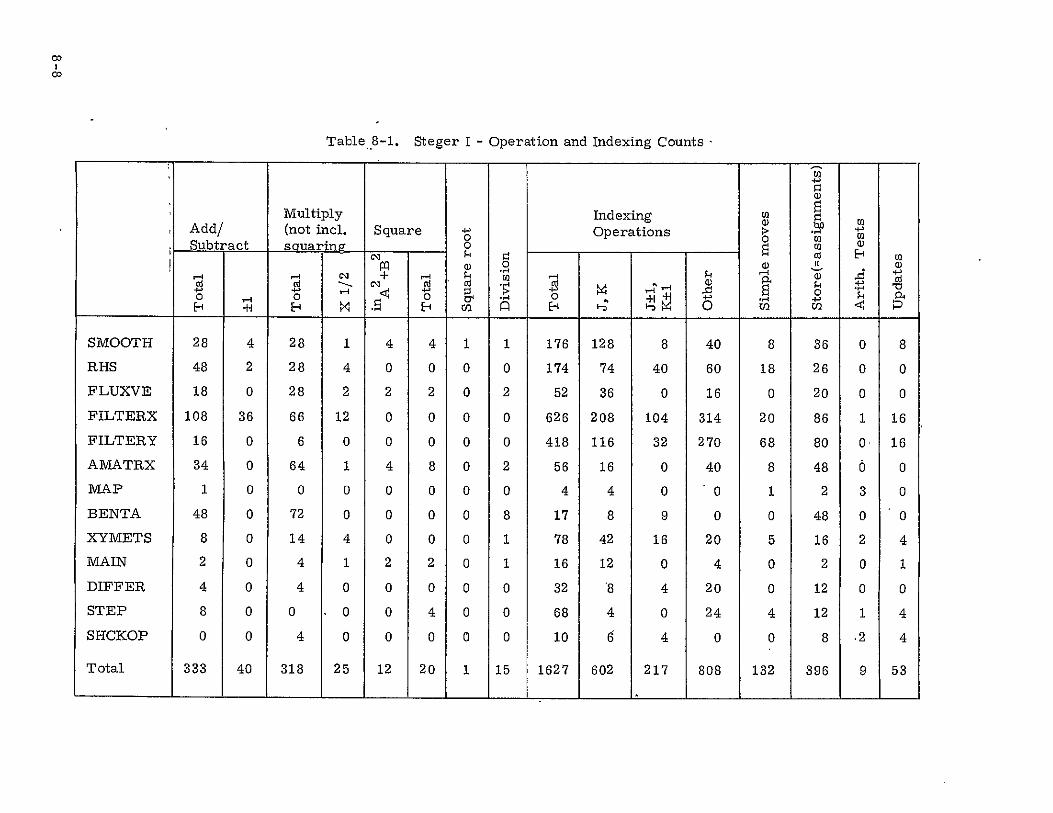
oD

Table.8-1. Steger I - Operation and Indexing Counts

__ __-H

Add/ Subtract

CU

Multiply (not incl. suaring

C13 Cd -.4-

- k<

Square _

m0 + -

dC +.

. E-

o

Cd to -0

0 FI

Indexing Operations

LAI4 -H

- 02q U

W

o

C

)

.

V

xi-3<I.

a)

4

SMOOTH

RHS

FLUXVE

FILTERX

FILTERY

AMATRX

IVAP

BENTA

XYMETS

MAIN

DIFFER

STEP

SHCKOP

28

48

18

108

16

34

1

48

8

2

4

8

0

4

2

0

36

0

0

0

0

0

0

0

0

0

28

28

28

66

6

64

0

72

14

4

4

0

4

1

4

2

12

0

1

0

0

4

1

0

0

0

4

0

2

0

0

4

0

0

0

2

0

0

0

4

0

2

0

0

8

0

0

0

2

0

4

0

1

0

0

0

0

0

0

0

0

0

0

0

0

1

0

2

0

0

2

0

8

1

1

0

0

0

176

174

52

626

418

56

4

17

78

16

32

68

10

128

74

36

208

116

16

4

8

42

12

'8

4

6

8

40

0

104

32

0

0

9

16

0

4

0

4

40

60

16

314

270

40

0

0

20

4

20

24

0

8

18

0

20

68

8

1

0

5

0

0

4

0

36

26

20

86

80

48

2

48

16

2

12

12

8

0

0

0

1

0,

0

3

0

2

0

0

1

.2

8

0

0

16

16

0

0

0

4

1

0

4

4

Total 333 40 318 25 12 20 1 15 1627 602 217 808 132 396 9 53

Table 8-2. STEGER I - Summary of Results

* Operation Distribution

46% * (8% of multiplications of form 1/2 X A) 48% ± (12% additions/subtracting form ±1)

2% divide 2. 6% in (A2 + B2 )

* Indexing Operations

2 indexing operations/floating point operation 1/2 of indexing operations to J, K loop variables 1/2 of indexing operations to small literals, i. e., N 20% of store instructions have identical indexing

* Intrinsics

1 SQRT in loop

* Operands

3. 53 input operand/output operand

8-9

Table 8-3. Steger II - Subroutine Structure

STEP

RHS FLUXVE DIFFER SMOOTX

K, J LOOP

FLUXVE DIFFER SMOOTY VISRHS

MUTUIR

J, K LOOP

FILTRX A MA TRX

BTRI LEJDEC

K, J LOOP

FILTRY A MA TRX

BTRI LUDEC

J, K LOOP

8-10

Table 8-4. Steger II - Operation Distribution for Major Subroutines (Steger)

# Times

Subroutine - MADD ± Called Comments

LUDEC 14 20 14 4 2

BTRI 144 160 144 0 2

VISMAT 89 67 10 2 1

AMATRX 15 43 4 1 2

FILTHY 16 6 4 0 1

FILTRX 12 6 4 0 1

SMOOTY 21 34 4 4 1

SMOOTX 21 34 4 4 1

MUTUR 23 38 6 15 1 6 Intrinsics

VISRHS 30 30 18 2 1

DIFFER 4 4 4 0 2

FLUXVE 9 16 7 1 2

RHS 4 0 0 0 1

Total 588 701 396 39 (totals-include frequency of times subroutine called)

56% of multiplies are participants in multiply, add operations.

8-1

Table 8-5. Data Base Memory Accesses and Floating Point Operation Distribution of Major Subroutines

Times #Floating* Fetch Store Tempor-

Subroutine Called Pt Operations EM EM aries Branches

LUDEC 2 35 0 0 20 0

BTRI 2 300 0 0 24 0

VISMAT 1 158 4 0 44 0

AMATRX 2 58 5 0 0 0

FILTRY 1 22 9 4 0 0

FILTRX 1 18 8 4 0 0

SMOOTY 1 63 0 4 1 0

SMOOTX 1 63 0 4 1 0

MUTUR 1 77 13 1 39 1 Mode

VISRHS 1 59 0 1 31 0

DIFFER 2 8 0 0 0 0

FLUXVE 2 26 4 0 10 0

RHS 1 4 2 0 3 0

Overall 1318 64 18 225

(weighted by times called)

* The Number of Floating Point Operations is for a given J, K point. The totals

include the frequency of times called.

8-12

Table 8-6. Percent Execution Time for Major Subroutines

Subroutines MNAX=50 Dependent on Iteration

LUDEX 2.74

BTRI 31.28

VISIVIAT 14. 82

AMATRX 4.99

FILTRY 9.94

FILTRX 7.84

SMOOTY 2.24

SMOOTX 2.66

MUTUR 6.32

EIGEN(1/5) 1.1

VISRHS 3.07

DIFFER 2. 61

FLUXVE 2.35

RHS 3.34

BC .57

Total . 97.3

STEP BTRI

LUDEG 64. 9% FILTRY

AMATRX VISVIAT

FILTRX AMATRX

(Not including IIHS)

NMAX= 10 (Normalized

to 50)

2.79

27.53

8.1

5.54

11.08

8.9

1.69

3.16

8.43

.6

5.54

2.22

4.42

7.89

.55

99.2

Code

NMAX=9 (Normalized

to 50)

1.7

23.07

9. 33

3.47

10.3

12.31

2.97

4.04

6.37

1.25

4.91

2.26

2.09

10.45

.36

96.5

RHS FLUXVE (2) DIFFER (2) SMOOTX SMOOTY VISRHS

MUTUR

MNAX=4 Average (Normalized

to 50)

2.01 2.3

24.57 26.6

9.35 10.4

6.23 5.1

12.47 11.0

8.98 9.5

4.9 3.0

3.1 3.2

7.51 7.2

.36 .8

3.66 4.3

1.26 2. 1

3.85 3.2

9.84 7.9

.36 .5

98.0 98

23% Code

8-13

Table 8-7. Memory Access, Floating Point Operations and Execution Time Comparison

Loop # Floating Subroutine Variable Point Calling Sequence

Outer/ Inner

Operation per JK pt Fetches Store % Execution Loop Totals

RHS 0 2 0

FLUXVE K/

26 .4 0 1. 6 6% code runs with 1 fetch (store)

DIFFER 8 0 0 1. 1 per 9. 7 floating

SMOOTX 63 0 4 3.2 point operations

Total 97 6 4 6.0

RHS 0 2 0

FLUXVE J/K 26 4 0 1.6

DIFFER 8 0 0 1. 1 17.2% code runs with 1 fetch

SMOOTY 63 0 4 3*.0 (store) per 9. 3

VISRHS 59 0 1 4. 3 floating point

MUTUR 77 13 1 7.2 operations

Total 283 19 6 17.2

BTRI

LUDEC

K/J 300

35

0

0

0

0

13.6

1.2

26. 8% code runs with 1 fetch (store) per 24. 2

FILTRX 18 8 4 9.5 floating point

AMATRX 58 5 0 2.5 operations

Total 411 13 4 26.8

BTRI 300 0 0 13.6

LUDECFILTRY J/K

3522

0 9

0 4

1.2 11i.0

38. 8% code runs with 1 fetch (store) per 26

A1IATRX 58 5 0 2.6 floating point

VISM1AT 158 4 0 10.4 operations

Total 573 18 4 38.8

8-14

Table 8-8. LOMAX Code Operation Distribution of Major Subroutines

Percent of No. Times Executing

Subroutine Called Code ± * / Branches Intrinsics

FILABC 1360 11.6 64 50 1 2 0

MMM4 2720 26.6 64 64 0 0 0

INV4 1360 19.3 48 92 1 0 0

MMV4 2720 6.7 16 16 0 0 0

VALF 4080 14.5 12 27 5 0

ELM 1360 6.7 32 32 0 0 0

FILEV 40 <1 9 35 7 8 (mode) (6 intrinsics)

Table 8-9.- MacCormack I Code Subroutine Structure and Calling Frequency

Main BC(1) TURBDA (NEND (conditional)) TMESTP (2*NEND) SETMBC (NEND (conditional)) LYH (2* NEND*MEND (conditional))

CHRVAL (I LMI*(i+2*(JKFM-1))) LY (1)

BC(1) G (ILMI +JE-JS)

(GADD(1) LIMBC (2 (card))

WEIGHT ((IL-I)*(5+ 2(conditional)))

LY (2*NEND and MEND (conditional)) (see calling tree for LY above)

LYP (NEND and MEND (conditional)) BC(1)

RSTMBC (NEND (conditional)) LY (NEND) - (see -calling for LY above under LYH) LX (2 NEND)

BC(2) F ((JE-JS-1) X ILMi)

FADD(1) PRTFLW (NEND (conditional)) REFINE( NEND (conditional))

BC(1) 8-15

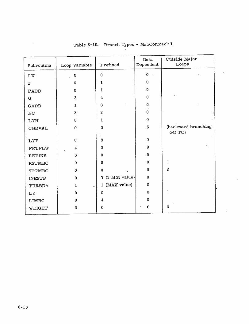
Table 8-10.

Subroutine Loop Variable

LX

F

FADD

G

GADD

BC

LYH

CHRVAL

0

0

0

3

1

3

0

0

LYP

PRTFLW

REFINE

RSTMBC

SETMBC

INESTP

TURBDA

LY

LIMBC

WEIGHT

0

4

0

0

0

0

I

0

0

0

Branch Types - MacCormack I

Data Outside Major Prefixed Dependent Loops

0 0

1 0

1 0

4 0

0 0

2 0

1 0

0 5 (backward branching GO TO)

9 0

0 0

0 0

0 0 1

0 0 2

7 (3 MIN value) 0

I1 (MAX value) 0

0 0 1

4 0

0 0 0

8-16

Table 8-11. MacCormack II Code Structure

with parameters NBDY=3, NSYM=O, ILJH=1, ILJP=1 ITURB=1, ISMTHI=2, ISMTHS = 2

Main MESH BC BDY3 PRNTFF TMSTP SHIFT (BC) TURBDA LI (PSI (FSIADD), BC) LJ (FSJ (FSJADD), BC) LJH (TMSTPF, CHRVAL, LJ (FSJ(FSJADD)), WKECNV)

LJP (BC) PRNTXY

Parameters indicate internal calls to Subroutines. Frequency

of calls dependent in run time parameters.

Table 8-12. MacCormack Code Calling Frequency for Specific Parameters

Specific Case NEND = 15 NVISC = 9 NBDY 3, NSYM = 0, 1 LJH = 1, ILSP= 1 JTURB = 1, ISMTHI = 2, JSMTHJ = 2

TURBDA 7 LJP 7 PRNTXY 1

PRNTFF 9 WKECNV 60 CHRVAL 26, 023 LJH 14 SHIFT 1 LJ 75 LI 44 FSJADD 67,392 FSIADD 95,256 FSJ 67, 392 FSI 95,256 TMSTPF 60 TMSTP 15 BC 314 MESH 1 BDY3 1

8-17

Table 8-13. MacCormack I Code - Percent of Execution Time for Major Subroutines

7 11 15 15 15NEND 4 4 7 9 3 13Subroutine NVISC = 3

LJP 5 5 4 5 6 6 5 5 5 6 4

PRNTFF 4 2 3 3 4 2 3 5 1 2 1

CHRVAL 3 5 3 3 3 4 3 3 3 4 -

LJH 6 3 2 3 3 3 3 3 2 4 5

SHIFT 8 7 7 - - - - 3 2 -

LJ 8 10 7 8 9 11 11 7 8 10 12

LI 15 13 16 14 15 16 15 18 18 15 19

FSJADD 4 5 5 5 5 6 6 5 4 6 5

FSIADD 7 8 7 7 8 8 7 7 7 6 9

FSJ 10 10 7 23 14 12 14 12 16 14 6

FSI 22 22 17 26 24 22 22 20 22 22 29

TMSTP - - 11 6 5 5 6 7 6 6 3

Total 92 90 89 93 96 95 95 95 94 95 93

Average

LI(FSI(FSIADD)) LJ(FSJ(FSJADD))

44 22

43 25

40 19

47 26

47 28

46 29

44 31

45 24

47 30

43 30

57 23

46 26 2-

All other Subroutines utilize less than 1 percent of the Total Execution Time.

Table 8-14. MacCormack. LI, LJ Subroutine Analysis

% LoopNo. of Floating Point Ops. * ± MADD Fetch Store Execu. TotalsSubroutine

40 8 46 46% codeLI(FSI(FSIADD)) 287 62 53 12 80 runs at 1 fetch/ 5. 7 variables

8 26 26% codeLJ(FSJ(FSJADD)) 199 55 39 15 45 34 runs at 1 fetch/4. 8

variables

Totals for code brought into line (eg. LI calls FSI which in turn calls FSIADD)

8-18

8. 2. 3 Discussion of Results

The list of characteristics shown on page 8-2 will be discussed in greater detail

below with reference to the program studies outlined previously.

The first and perhaps most significant characteristic of the programs is the low

interaction of the computational variables on different grid points. This is the

program attribute which suggests an architecture that has vertical slicing. The

first loop presented below has a low interaction between computational variables

while the second does not.

Do 1 J=2, JIVIAX Do 1 I=1, IVIAX A(I, J) = XY (I, J+l) * Q(I, J+1)

xY (I, J-D * Q(I, J-1) D (I) = A(I, J)*HD+F(I, J) R (I) = A(I, J) + F(I, J)

1. CONTINUE

Do 2 J=2, JMAX Do 2 I=1, JMAX A(I, J) = XY (, J+I)*Q(I, J+1)-

XY (I, J-I)*Q(I, J-1) D(l) = A(I, J+1)*HD+F(, J) R(I) = A(I, J-1)+F(I, J)

2 CONTINUE

In the loops,the underlined array accesses are from the data base. An array

element A(I, J) is created and then utilized in subsequent statements. In the second

loop,the element A(I, J) is created in one statement and A(I, J+l) and A(I, J-1) used

in subsequent statements. This implies other fetches from memory in order to

obtain the A, J+1) elements when the last two statements are executed for the

SAM,where each particular (I, J) value has been assigned to a specific processor.

In general, for both the Steger and Lomax codes array elements once created within

a loop were utilized repeatedly, with little skipping around in a created array.

These results were obtained by inspection of all subroutines of both programs. Hence,

once having obtained the elements from the data base, one is able to perform all

8-19

the computations without accessing external array elements. In the second loop,

one would calculate all elements of A(I, J) in the first statement, then use the old

values of A(I, J) in the second and the new values in the third. That type of loop

suggests a "horizontal slice" architecture.

The second characteristic of the programs, which, in a sense, follows from the first is that there are relatively few fetches and stores from the data base relative

to the number of floating point operations. This characteristic is shown in

Table 8-7 for the Steger II code and Table 8-8 for the MacCormack II code.

Approximately 66 percent of the Steger code has 25 floating point operations per

fetch or store from the data base and 23 percent has 9 floating point operations

per fetch or store. In the MacCormack program, 72 percent of the code has 5

floating point operations per fetch or store. The remaining I I percent in the

Steger Codelappears to have at least 10 floating point operations per fetch or store

while the remaining 28 percent of the MacCormack code appears to have at least

5 floating point operations per fetch or store from the data base, although not as

extensive an analysis was performed. However, these other portions of the code

are expected to execute a smaller proportion of the total time as NMAX and NEND

increase. As noted previously, rarely executed subroutines represent an extremely

high percentage of the execution time due to the B 7700's monitoring procedures.

Another characteristic devolving from the first and second is the relatively high

temporary-propagation per datum fetched or stored. It follows that if few accesses

are made to the data base and a lot of computation occurs, intermediate results

are stored temporarily. This suggests a vertical slice machine, as the temporary

storage is grid-independent and the "temporary blow-up" that occurs on horizontal

sliced architectures can largely be avoided. In Table 8-5 the temporary storage

was counted for the individual subroutines. If one was considering each floating

point operator as being part of a dyadic operation with 2-operand input and a single

result, then the number of temporaries produced for the FILTRX(AMATRX) BTRI

(LUDEC) portion of the code would be 411, while the RHS including SMOOTX, DIFFER,

FLUXVE would be 97. This volume of temporary propagation could be horrendous

if not handled properly by the programmer and a smart compiler.

8-20

A count of the number of input operands per assignment statement for the Steger I

programs disclosed 3. 53 input operands/output operand. For the explicit portion

of the Steger II code, the count was 3. 2. Since this code has a large number of moves

to temporary arrays, this implies that many assignment statements have four or

more operands. While scientific programs in general have a large number of

operands per statement, this result appears to be higher than average.

The branch structure was examined for both the Steger and MacCormack codes

and found to be relatively simple. Only subroutine MUTUR in the Steger II pro

gram has several branches. Depending on the type of architecture they can be

handled in a variety of ways. The rewriting of this subroutine for a parallel

machine would be highly machine dependent. The Branch types for the MacCormack

II code have been presented in Table 8-10. Subroutine CEIRVAL, constituting

4 percent of the program's execution time, also would have to be rewritten for a

parallel machine. In general, it was found that the branches were run time para

meters, loop variables, or otherwise prefixed before loop execution.

Recurrence relations- only appeared in the BTRI subroutine of the Steger II code.

However, these recurrences, which are extremely comples first order linear

recurrences, were nested inside other loops where they can be computed efficiently.

In principle all parallel machines can handle recurrences to some degree even when

nesting does not occur. Some architectures will be required to do transposes and

other copies in order to enhance the parallelism. The scalar code appearing in

MUTUR is similarly nested and can be executed well on array machines.

The frequency of "Multiply, add" in the programs (see Table 8-4) suggested

that the ultimate design be optimized to handle that operation extremely efficiently.

A recurrence relation is defined by

A. =B i + C *A 1.<i<N

It has been shown that, on a parallel machine with N processors, recurrence relations need take only log2 (N) steps.

8-21

8. 3 PERFORMANCE OF THE SYNCHRONIZABLE ARRAY MACHINE MEASURED AGAINST EXISTING CODES

8. 3. 1 Code Discussion

The FORTRAN Loops presented in F. R. Bailey's letter of July 7, 1977 provide

a convenient vehicle for discussing parallel languages as well as a means for

showing the performance of the SAM.

The given loops are to be considered as a unit - that is, in some code they follow

directly after one another.

FOR ALL I, J, K DO B(1:3) = A(:3, I, J, K) C = A(2, 1+1, J, K) LOOP 1A D = A(2, I-1, J, K) E = B(2) + B(1)*(C-D) A(2, L J, K) = E*B(3)

FOR ALL I, J, K DO B(1:3) = A(1:3, I, J, K)C = A(2, L J+, K) LOOP 1B

D = A(2, L J-1,K) E = B(2) + B(1)*(C-D) A(2, I, J, K) = E*B(3)

8-22

For clarity in discussing various architectures, they are recast below (in two

versions) in Serial ANSI FORTRAN which show different data dependencies.

1 DIMENSION A(5, 100, 100, 100) F(100), B(5) 2 DO 1 K=1, 100 3 DO I J=1, 100 4 DO 2 I=2, 99 5 DO 3 N=I, 3 6 B(N) = A(N, I, J, K) 7 3 CONTINUE 8 C = A(2, I+l, J, K) 9 D = A(2, I-1, J, K) LOOP 2A

10 E = B(2)+(B(1)*(C-D) 11 F(I) = E*B(3) 12 2 CONTINUE 13 DO 4 I=2, 99 14 A(2, I, J, K)=F(I) 15 4 CONTINUE 16 1 CONTINUE

17 DO 11 K=l, 100 18 DO 11 Il, 100 19 DO 12 J=2, 99 20 DO 13 N=1, 3 21 B(N) = A(N,I, J,K) 22 13 CONTINUE 23 C = A(2, I, J+1,K) Loop 2B 24 D = A(2, I, J-1,K) 25 E = B(2)+B(1)*(C-D) 26 F(J) = E*B(2) 27 12 CONTINUE 28 DO 14 J = 2, 99 29 A(2, 1,J, K) = F(J) 30 14 CONTINUE

The reason for transcribing the "FOR ALL" parallel statement in this manner

with the extra temporary array F is that one is using all the "old" values of

A(2, I-1, J, K) in line 9. This is one interpretation of the parallel statement, which

can be described as "anti data dependence. " It is necessary to introduce this

temporary into the serial ANSI FORTRAN in order to produce the same results.

(Note also that J ranges from 2 to 99 so as not to exceed Array dimension when

I-I and I+1 accesses are made.)

8-23

A second interpretation is to assume that an updating of the results occurs on each

I interation and that this is in fact a recurrence relationship.

1 DIMENSION A(5, 100, 100, 100), B(3) 1 2 D DO 1 K=1, 100 3 DO 1 J=l, 100 4 DO 1 I=2, 99 5 DO 3 N=1, 3 6 B(N) = A(N, I, J,K) L

LOOP 3A7 3 CONTINUE 8 C = A(2, I+, J, K) i Recurrence on I

9 D = A(2, 1-1, J,K) 10 E = B(2)+B(1)*(C-D) 11 A(2, I, J, K) = E * B(3) 12 1 CONTINUE 13 DO 11 K= 1, 100 14 DO III= 1,100 15 DO 11 J = 2, 99 LOOP 3B 16 DO 13 N = 1, 3 Recurrence on J

17 B(N) = A(N, I, J,K) 18 13 CONTINUE 19 C = A(2, I, J+, K) 20 D = A(2, I, J-1, K) 21 E = B(2)+B(I)*(C-D) 22 A(2, I, J, K) = E*B(3) 23 11 CONTINUE

LoopilIA-B could also be rewritten in more compact form yielding the identical

results as 3A-B as follows:

1 DIMENSION A(5, 100, 100, 100) 2 DO I K=1, 100 3 DO I J=1, 100 4 DOII=2,99 LOOP 4A 5 A(2, I, J, K) = A(3, 1, J, K)*(A(2, I,5, K) + 6 A(I, I, JK)*(A(2, I+, J, K)-A(2, I-I, 5, K))) 7 1 CONTINUE 8 DO 11 K=I, 100 9 DO 11 I=1, 100 10 DO 11 J=2, 99 LOOP 4B 11 A(2, 1, J, K) = A(3, 1, J, K)*(A(2, I, J, K)+ 12 A(1, I, J, K)*(A(2, I, J+1, K)-A(2, I, J-1, K)) 13 84 CONTINUE

8-24

Note that the updating of element A(2, I-1, J, K) on each iteration in statement 5-6

becomes obvious in this representation. This "data dependency" has to be

handled in all parallel machines. No data dependency exists on J or K in

Loop 4A.

Loops written in this compact form result in less temporary array propagation

for various architectures.

The cited loops are not truly typical of the Navier Stokes problem in the sense

that there is much more fetching from the data base than is found in actuality in

the Lomax-Steger or MacCormack code.

8. 3. 2 Synchronous Array Machine (Compilation and Execution of Sample Loops

Taking loops 2A-B as the ANSI FORTRAN version of Loop lA-B these would be

written in the following form for the SAM for optimum machine utilization.

DIMENSION A(5,100,100), B(5), F(100) 1 DO PARALLEL K=1, 100 2 DO PARALLEL J=1, 100

3 DO 2 1=2,99 4 D = A(2, I-1, J, K) 5 C = A(2, I+l, J, K) 6 DO 3 N=1, 3 7 'B(N) = A(N, I,-J, K) Inner Core Code

8 3 CONTINUE 2A 9 E = B(2)+B(1)*(C-D) 10 F(I) = EB(3) 11 2 CONTINUE 12 DO 4 I=2, 99 13 A(2, 1, J, K) = F(I) 14 4 CONTINUE

15 END DO 16 END DO 17 DO PARALLEL K=1, 100 18 DO PARALLEL I=l, 100

8-25

19 DO 12 J=2, 99 20 D = A(2, I, J-I, K) 21 C = A(2, I, J+1,K) 22 DO 13 N=1, 3 23 B(N) = A(N,I, J, K) Inner Core Code 24 13 CONTINUE 23 25 E = B(2)+B(1)(C-D) 26 F(J) =.E*B(3) 27 12 CONTINUE 28 DO 14I= 2 , 99 29 A(2, I, J, K) = F(J) 30 14 \CONTINUE

31 END DO 32 END DO

The code compiled for the SAM for the processors would only involve the state

ments within the DO PARALLELS since the outer two loops constitute the plane

of computation being fed to the 512 PEs. One can think of the inner loops being

transformed as follows for the first set of loops with suppression of the J, K

indexing leaving only the I, N indexing:

DO 2 I=2, 99 D = A(2, I-1) C = A(2. I+1) DO 3 N=1, 3 B(N)= A(NI Inner Core Code

3 CONTINUE 2A E = B(2)+B(1)*(C-D) F(I) = E*B(3)

2 CONTINUE DO 4 I=2, 99 A(2, I = F(J)

4 CONTINUE

It should be noted that the expressions for C and D have been moved ahead of the

loop for B(N). This was done because the access of A(2, 1-1,5, K) from Extended

Memory only has to occur for I=2. All other I indices 1have been previously

moved from Extended Memory into PE Memory via DO 3 loop. The move of

A(2, 1+1, J, K) from Extended Memory to PE Memory must be done for each

iteration. As a result there are four Extended Memory loads and one Extended

Memory save for Loop 2A. (underlined quantities)

8-26

Since each PE operates on this segment of code in a serial fashion for these

innermost loops one can think of the machine as "vertically" slicing through the

code instead of "horizontally" slicing as in a lock step array or pipeline machine.

In terms of access to Extended Memory the cycle of computation is

"FTPPPPPPTS" F=fetch T=transpose, P=process, S=save) series.

Table M-1 shows the code for the first half of loop 2, as hand compiled.

Note that accessing array elements from extended memory are:

LOC EM(J, K) = 1921 (N-I)+I

LOC PEM = 5*(I-I)+N

This is because the A (5, 100, 100, 100) array in Extended Memory is stored as

5 subarrays of 106 each, so that, for a given I, J, K, each N has in the same

memory module 1921 apart (521 X 1921 = i000841).

The hand compilation was performed very conservatively. Each access to the

A array was indexed in Extended Memory and PE Memory and then moved from

EM to PEM, than it was moved from PEM to a register and from there the

assignment statement was executed with a save to PEM with the new variable

name. It never assumed a smart compiler that would realize that the A(2, 1+l, J, K)

element was used only once when assigned to C and hence moved it from EM

directly to a register. The performance ratings are therefore very conservative.

8-27

Table 8-15. Code for SAM

Loop Inst. CU PE Register Name No. Inst. Inst. Allocation Comments

1 SETL=20 2 WAIT

Li: 3 LOOPC 4 SETL £0, 1921 LOC EM = 1921(N-1)+I reg contains skip 5 SETTN SETL Ii, 5 LOC PEM = 5(I-1)+N reg contains skip 6 IADDL 13, 10, 1 'Address A(2, 1, J, K) in EM 7 LOADEM 13, 2, £0 The five fields are as follows

II, 1,A 1 EM address (reg or literal) of ist one 2 PEM address (reg or literal) of ist one 3 Skip (reg. or literal) 4 Skip (reg. or literal) 5 Number to be loaded

8 SETL 12, 2 I index 9 SETL 14, 99 Loop limit

L2: 10 IMUL 5,I2,Ii .form 5*(I) 11 ISUBL I9, 15, 8 form 5*(I)-8=address A(2, I-1) 12 IADD 15, 10,12 Address A(2, I+I, J, K) in EM

formation form (1921+1) 13 INCR I5, I5, 1 1921*+1 = Address (2, 1+1, J, K) EM 14 IMUL 16, 12, II form 5* 1 PEM Address A(2, I+1) 15 FETCH RO, 19, 0, A fetch A(2, I-1) 16 STORE RO, 0 Store D 17 LOADEM I5, 16, 10,

I,I1, A .18 19 20 2SETTN

DECR IMUL FETCH

17, 12, 1 17,17, Ii RI, 16, 2A

form (I-1) form 5*(I-1) Fetch A(2, 1+1) from PEM

21 STORE RI, C 22 23

INCR LOADEM

I7, I7, 1 12, 17, I0,

from 5*(I-I)+i address A(N, I) in PEM stream 3 values of A(N, I, J, K) into

I1, 3, A PEM 24 FETCH R2, I7, 0, A A(I, I) from PEM 25 STORE R2, 0, 1, B B(1) 26 27

FETCH STORE

R3, I7, 1, A R3, 0, 2, B

A(2, I) B(2)

28 29

- FETCH STORE

R4, I7, 2A R4, 0, 3, B

A(3, I) B(3)

30 31-32

SUB MADD

RI, R1, RO Ri, R3, R2,

(C-D) B(2)+BI*(C-E)

Ri 33 STORE RI, E

-28

Table 8-15. (Cont'd)

Loop Inst. CU PE Register Name No. Inst. Inst. Allocation Comments

34 MUL Ri, Ri, R4 35 STORE RI, 12, F Store F(2) 36 INCR 12, 12, 1 37 TEST L2, 12,14 BRANCH to L2 38 SETL 12 39 SETL 14, 99

L3: 40 FETCH - RO, I3, F 41 IMUL 15, I=1, IS 5*(I-1)+2) 42 ISUBL I,15, 3 43 STORE RO, I5, A A(2, I) in PEM 44 IADD 16,10,13 Address in EM A(2, I, J, K) 45 SAVEM 16, 15, I0, IS,

IA 46 INCR 12, 12, 1 47 TEST L3, 12, 14 48 WAIT wait on CU Test 49 CUINCR

CUTEST

8-29

The mnemonics used in the instruction set vary slightly from those names used

in Chapter 4. At this juncture they are used only as representative of a reasonable

subset of the possible instructions.

SETL Set literal in integer register IADDL Add literal to integer register and place in integer register ISUBL Subtract literal from integer register and place in integer register

IADD Add one integer register to another and place in third ISUB Subtract one integer register from another and place in third IMUL Multiply 2 interger registers and place in third IMULL Multiply I integer register by literal'and place in third INCR Increment by literal' DECR Decrement by Literal FETCH Fetch from PE memory, with using index register for location

STORE Store to memory, with using index register for location LOADEM Fetch from extended memory into PE memory (further

explanation below) SAVEM Store to extended memory from PE memory SUB Subtract one floating point register from another and place in third

ADD Add one floating point register from another and place in third

MUL Multiply one'floating point register from another and place in third

MADD Add two floating point registers together and multiply by third and place in fourth

TEST Test two integers; if test fails branch

A score board will keep track of the availability and utilization of the various

functional units within each Processing Element to permit effective overlap

and efficiency of the units. A time line chart of the utilization of the various

units is diagrammed on an instruction-by-instruction basis in Figure 8-1.'

The calculated MOP rate on this loop (2A) is determined below:

start up before L2 - 20 clocks 98 interactions *(139-23) 11017 start up before L3 - 3 98 iterations*(161-142) = 1862

12902 clock = . 516 X 10-3 sec

-X20 outer loop iterations (J, K) = 10. 32 X 10 3 sec

= 4 X 98 X 10, 000 = 3. 92 X 106No floating point ops

MOPS - # floating pt ops 3. 92 X 106 = 380 MOPSexecution time 10. 32 X 10-3

8-30

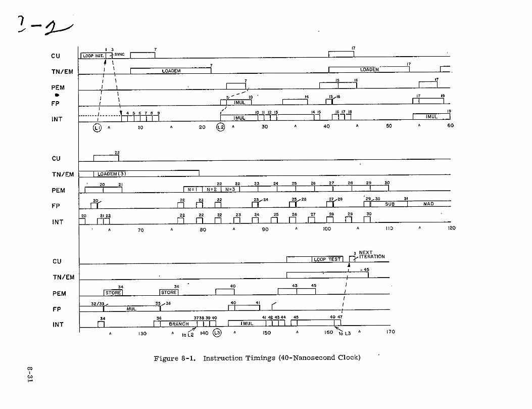
7S7

CuI LOOP I iiSNCF\

I LOADEMTN/EM I LOADEM 7 ] 16

PEM IF_-1 071 0I 4 16

5 6 7 8 ]MUL I 10 II 12 t3 -- 17 16 17 18INT . .4 I....-- 777I 91 I--]77 14 15 177rIU

0 A 20 A 30 A 40 A

CU

TN/EM I LOADEM (3)

22 23 25 27 2920 2t 22 24 26 28

PEM rI= , I I I j 24

22 222 ~ 2526 2728 29-30

FP Fff F9 F9 Yl FT I U

26 3020 21 22 22 22 22 23 24 25 27 28 29

INT 1 M D F- r- M F7 r- D M 0 El F7 A 70 A so A 90 A 00 A

SNEXT

I ILOP TEST I r -ITERATION CU A

S -45 -I

TN/EM 34 36 40 43 45

PEM _TEI STORI FF FP 32/33I MUL I3 6 40I/ 41I7 --

36 37383940 41 424344 45 40 47

INT 34

III BRANCH I I IMULT 17-- 1 1 I,oo o L,to L2 140 @ 15 ^t, A 160s 3 A17A 130 A to2 5

Figure 8-1. Instruction Timings (40-Nanosecond Clock)

0003 I

17

50

7 19

19

60

30

UuW 31

AD

110 A 120

Both loop 2A and 2B run at the same MOP rate.

Temporary propagation for Loop 2A assuming data stored in PEM

for each I iteration.

512 X D +B(1) + E + F -12X512 =Gl44addresses+C + B(2) + B(3)+A(2, I-1), A(2, I+l) + A(2, I) + A(1, I) + A(3, 11 inEM

It has been shown in the typical Navier-Stokes programs that the ratio of floating

point operations to fetches and stores from Extended Memory will exceed 10:1.

seems reasonable to introduce, artificially, more floating point operationsThus, it

into the loops to generate test cases for calculating throughput as a function of

that ratio.'

This was done by first looking at the instruction mix for floating point operations

in the Steger code (using Table 8-4 to generate Table 8-16).

From Table 8-16, 100 floating point operations take 29, 470 ns, giving, in all 512

processors, 1. 74 X 10 floating operations per second, based on the observed

instruction mix. The maximum possible, based on everything being multiply

add instructions, would be 2. 33 X 109 floating point operations per second.

Note that this is based on the assumption that all PE's are busy.

For a more realistic estimate, it was further assumed, conservatively, that

there would be one non-overlapped fetch and one store to PEM for every four

floating point operation, resulting in 35, 470 ns or 887 clocks for one hundred

fully executed floating point operations per PE including all allowances for PEM

activity of 6050 ns.

Inserting 50, 100, and 200 floating point operations in each of the two loops, 2A

and 2B, yielded Table 8-17. This includes the EM activity previously included in

the loop execution time. From the data in Table 8-17, Figure 8-2 was generated.

The data in the Code Characterization Section, Tables 8-7 and 8-14, was then

used to determine expected performance.

8-32

Table 8-16. Instruction Mix

Execution Relative Time Execution

Occurence Ratio (Nanosec) Time

± (Not in IVADD) 192 .1452 240 34.8

(Not in MADD) 305 .2307 360 83.1

(In MADD) 396 .2995 220 65.9

± (In MADD) 396 .2995 220 65.9

33 .0250 1800 45.0

294. 7 ns/floatingpoint

Average Execution Time/PE

Table 8-17. Throughput vs. Loop Length

Floating Point Operations Total Inserted Inserted/Loop in Both Loop MOP Rate

50 100 1140

100 200 1260

200 400 1320

8-33

MacCormack (72 Percent Code)

Explicit Steger II (23 Percent Code)

1500 Implicit Steger II (66 Percent Code) SAM

0

0

1000 0

0

0

0

.-500

lO 20 30 40 50 6o 7o 80

No. of Floating Point Operations.One Fetch (store)

Figure 8-2. Expected Performance on Characteristic Programs

8-34

8. 4 ADDITIONAL ARCHITECTURE EVALUATIONS

8. 4. 1 Summary

Paragraph 8. 4 is an evaluation of the baseline system against a list of require

ments submitted by NASA.

8. 4. 2 Throughput Measured Against Given Parameters

Table 8-18 is a restatement of information furnished by NASA. The relevance of

the data in this table to parameters of the NSS design is discussed item by item

in the following paragraphs.

8. 4. 2. 1 EM Size

The 15 million word typical data base is easily held within the 34-million word EM.

8. 4. 2. 2 NSS Throughput

NSS throughput estimates, discussed in paragraph 8. 3, come to 2. 33 X 109

(best case), 1. 7 X 109 kexpected instruction mix), or 1. 34 X 109 (typical loop

including characteristic fetches and stores from EM) floating point instructions

per second. The 10-minute steady state solution and the 60-minute quasi-steady

state solution times have been estimated by NASA to require a machine of at least

1. 0 X 109 floating operands produced per second.

8.4. 2. 3 EM to DBM Transfer Rate

The design contemplates a transfer rate of one 48-bit word of data (plus check

bits) every 400 ns, or 2. 5 X 106 words per second.

Loading configuration geometry, item 1. A in Table 8-18, requires moving

3 X 106 words and takes 1. 2 seconds.

Loading a restart 5 X 106 words item 1. B, takes 2 seconds if the data is in the

form of 48-bit words. If data is packed in the form of two 24-bit words per

48-bit word restart, it takes only I second.

8-35

Table 8-18. Flow Simulation Processor 1/0

Assumptions

5 X 105 Grid Points

5 Conservation Variables (2 time levels)

2 Turbulence Variables (2 time levels)

3 Grid Coordinates

9 Grid Metrics

1 Jacobean, totalling:

about 15 X 106 words

minutes per steady state solution starting from previous caseabout 10 about 60 minutes per quasi-steady solution.

Types of I/O

1. Job Loading

A. Zero Base Start

Load configuration geometry, angle of attack, machine number,

Reynolds number, etc. Remaining data is machine generated.

B. Restart

Load zero base start plus five conservation variables, 'two turbulence

variables, and three grid coordinates per grid point.

10X 5 X 105 = 5X 106 words.

2. Job Unloading

A. At end of steady case it will unload restart dump of about 10 variables/ reduced data in thegrid point or 5 X 106 words. It will also unload some

form of:

the form of lift, drag, and moment coefficients.1. Integrated pressures in

2. Data for body surface contours, 10 variables per surface grid point.

Surface = total - grid/50, therefore about 105 words.

B. Long jobs (over 20 minutes)

Unload restart dump every 10 minutes (approximately).

3. Snapshots

A. Steady Case

and moment coefficientsEvery 15 seconds, output: time step, lift, drag, Surface pressure coefficient, about. 104

order to monitor convergence.in words, is also desirable.

B. Unsteady Case

Same as steady case plus surface contour information every 15 seconds,

or 105 words every 15 seconds; 24 X 106 words per 1 hour run.

8-36

Restart dumps, 5. 1 X 106 words item 2. A, likewise take I or 2 seconds. The worst interference possible from all of the above is 5. 2 seconds every 10 minutes.

Steady case snapshot dumps, item 3. A, are 104 words takine 4 ms every 15

seconds.

Unsteady case snapshot dumps, item 3. B, 105 words, or 40 ms, every 15 seconds.

8. 4. 2. 4 DBM Size

The DBM contains the data bases being readied for the next job. Interactive and multiprogramming host operations may result in more than one next job being readied at once. Besides the next job, the DBM contains areas allocated to the current job and to the results of the last jobs run, until the host-can get around to them. Therefore, the bare minimum size foriDBM is three maximum-sized

restart dumps. Typical restart dumps are 5 X 106 words (possibly 24 bits each, if packed two per 48-bit word). Without depending on the packing of 24-bit words and with allowing a factor of three for maximum job size vs. typical job size yields 2. 5 X 109 bits a minimum DBM size. The CCD design for the DBM, as shown in Chapter 3, has 7.38 X 109 bits.

8. 4. 2. 5 PEM Size

Analysis of temporary variables in the block tridiagonal code shows that about 75 variables are generated per grid point on the sweep in one direction down the computational grid. With a grid extent of 100, this results in 7500 addresses being used for this one function. These temporaries appear to dominate the

memory requirements. Sixteen thousand words are in the design.

8.4. 2.6 PEPM Size

Overlay, from CU memory, of program runs very fast. Hence, the PEPM need only be big enough to hold the central iteration of the program. The central iteration in Steger II (MAIN, STEP, and RHS and all the subroutines that are called, directly or indirectly, from them during the central iteration), taken from the listing of March 28, 1977, is 4, 607 words. Not counting unused subroutines, the code files contain an additional 3587 words of code.

8-37

The code file size of the PEM code in the NSS will be different from the above,

which is for the CDC 7600 computer. Some of its operations will not be found in the

PE code. For example, global operations are done in the CU instruction stream;

indexing that is implied byPE number in the NSS is explicit indexing in the 7600.

One suspects the PE code file may be shorter than the 7600 code file for comparable

subroutines.

A PEPM size of 8, 192 words would appear to be adequate to support any reasonable

NASF program, with at most two overlays per production run, one following

initialization to bring in the main iteration and one after the last iteration for

the clean-up code.

8. 4. 2. 7 CU Memory Size

CU memory must contain both the PE and CU programs; PE because the CU mem

ory will be the source for overlaying. The sum of the two programs is probably

larger than the code file used by the 7600 for comparable programs. Some

portion of the operating system is resident on the CU, as well as confidence checks.

Since the sum of the code lengths above (for the CDC 7600) is 9194 words, it is

clear that 16K is too small for the CU memory, wherefore 32K has been selected

as the size.

8-38

8. 5 OTHER ASPECTS OF ARCHITECTURE COMPARISON

This paragraph describes a compendium of comparisons of the syncronizable

array machine as exemplified by the baseline system, against the other architectures,

on the basis of a number of criteria. Table 8-19 summarizes the findings. The

Synchronous Array of the baseline system and the Lockstep Array, come out

approximately equal on most counts. The Lockstep Array is assumed to contain

any appropriate useful features of the baseline system such as the transposition

network. Appendix L shows a more careful analysis of the comparison between

the baseline system and a lock-step system that is similar to the baseline system

in most respects except for the independent instruction decoding.

In the case of the pipeline system, solutions have not been found for some of the

problems that the baseline system solves. For example, the transposition net

work provides transposed data, with no time spent in programmed transposition.

In the pipeline system no method has been found for handling the transposition

problem without costing throughput.

8. 5. 1 Data Allocation and/or Rearrangement

For both Lock Step Array Machines and Synchronous Array Machine, many solu

tions to the data allocation problem are shown, in Chapter 4 and appendix A,

where no time is spent in transposition.

For the Pipeline Array Machine, when transposed data is desired, data can be

fetched to the buffer registers, and it can be stored back to memory in trans

posed form. Alternatively, bit vectors can be set up that cause the pipe to

operate only on every pth element of the vector, obtaining, at reduced through

put, the same effect as the Synchronous Array Machine achieves by fetching

every pth address from EM. In either case, the Pipeline Array Machine loses

throughput whenever transposed arrays are used.

8-39

Comparison Issue

,Data Allocation/ Transposition

Interconnection Schemes

Temporary Propagation

Programmability

Irreducible Non-Concurrency

Parts Count

Accuracy

Throughput

Error Control

Performance as General-purpose

Note 1

Table 8-19. Four Architectures

Synchronizable Lockstep

Takes zero time See Chapter 3 TN description

Solved, as above or in Appendix B

OK. OK

Acceptable Acceptable

Not a Not a problem problem

Appeoximately the same for either

OK OK

1. 7 Gflops About the same as SAM

All design Instruction options open retry not

possible

Limited, Limited but better than lockstep

Compared

Pipeline

Takes time (Note 1)

Solved

Depends on compiler, affects throughput

Not Determined

Not a problem

Not D etermined

OK

(Note 1)

Instruction retry not possible

(Note 1)

Hybrid

Unsolved

Unsolved

Not Applicable

Very poor

(Note 1)

Very low

Unacceptable

High

Very poor, unacceptable

None, bad

The effort expended in this study has failed to find satisfactory solutions to the problems represented by this entry.

8-40

8. 5. 2 Temporary Propagation

In many computations, temporary variables are allocated to hold intermediate 11

results. Things that may be a single temporary variable inside a DO loop on a

serial machine may need to become a vector of temporary variables in a parallel

machine.

In an array machine (using, as an example, input source suitable for the SAM)

consider the following source:

DOPARALLEL 10 J=1, 100 DOPARALLEL 10 K=2, 50 DO, 10 L=2, 99 B=A(J, K, L) C =A (J, K±L+1) D=B+C-COSA A(J, K, L) = B+D

10 CONTINUE

The source code says that all 4000 instances of (J, K) index pairs can be done

simultaneously in parallel. Although this seems to imply that 4900 instances of

B, C, and D are required, any reasonably smart compiler will know that there

are only 512 processors, and that therefore he needs only 512 different B's, one

per processor, 512 C's, and so on.

For the pipeline machine, the source code will be different. If the two-dimensional

array A has been equivalenced to a one-dimensional array AA with extent 4900,

the compiler may emit vector statements that require temporary vectors that

are 4900 elements long. If not, then perhaps shorter temporary vectors can be

used. Different ways of writing the program, and different compilers, will

produce different amounts of temporary propagation. However, in the pipeline

machine, the use of shorter vectors, which reduces temporary propagation, will

also reduce throughput because of startup time. See Figure 8-3 for a plot of

startup time versus vector length.

Temporary propagation is therefore a function of both architecture and compiler.

In the case of the baseline system, the compiler cuts the parallelism into

512-sized pieces, and temporary vectors are never longer than 512 elements.

8-41

THROUGHPUT (AS TO AFFECTED BY STARTUP TIME)

t LT=S L, Vector Length

(Proportional to Amount of Storage taken up by Temporaries)

Figure 8-3. The Tradeoff Between Temporaries and Throughput in Pipeline Architecture

8-42

8. 5. 3 Interconnection Schemes

Data paths must be provided so that the data produced in one part of the computa

tion can be brought back into place for computation with other variables. The

transposition network - 521 switchable connections of 400 X 106 bits per second

each - provides the intercommunications facility for the baseline system. The

network can be adapted to a Lock Step Array Machine as well.

A Pipe Line Array Machine contains some number of pipes. If an array of pipes

is constructed with each pipe assigned to a piece of the same vector, each long

vector, split up among 20 pipes, is only 5 percent of the normal vector length.

If the vectors are to be kept long, then the several different pipes in the Pipe

Line Array Machine must be streaming different vectors. Either they are chained,

with attendent compiler complexity, or they are streaming in and out of separate

memory banks. If there are many banks, the compiler would optimize the assign

ment of vectofs to memory banks in such a way that following statements find mini

mum bank conflicts. The multiplicity of banks implies a fragmentation of memory

allocation that could be difficult for the compiler to handle.

8. 5. 4 Programmability

A compiler for the Lock Step Array Machine will be an extended FORTRAN. The

preferred data allocation scheme for the Navier-Stokes Solver is built into the

compiler, so that algorithms using this preferred scheme do not have to allocate

data by hand.

The Synchronous Array Machine has wider hardware options than does the Lock

Step Array Machine. These options result in more efficient running, but they

also mean that more decisions are made at compile time. For example, a loop or

subroutine can be executed' synchronously, with all PEs finishing theit part of the

loop before the next iteration starts, or the loop or subroutine can be executed

independently in every PE. Thus, there are two kinds of branches, the within-PE

branch and the synchronous branch. In the input language, different constructs

are needed if the programmer is to control these differences; but the language

8-43

allowshim to ignore them When control does not matter. Thus the Synchronous

Array Machine has more options in the input language, corresponding to the wider

latitude of choices as to how things are to be done.

Programming for a group of pipelines will have features that depend on the way the

pipelines are combined to cooperate on a single problem.

Programming of the Hybrid machine is a completely different art than the writing

of digital programs. At this writing, we do not know how to program a hybrid

architecture NSS.

8. 5. 5 Irreducible Non-concurrency

A major worry of every beginning user of a parallel machine is that his programs

will be X percent serial, and that therefore, no matter how many processors

he puts in parallel, X percent of the code will be running on a single serial pro

cessor, limiting throughput. A careful scrutiny of both codes submitted to

Burroughs by NASA-Ames shows that this worry is baseless for the NSS using

any N up to 512. Much less than 0. 1 percent of the code is of the irreparably

serial type.

8. 5. 6 Parts Count Comparison

On the basis of concurrency, the Synchronous Array Machine should need fewer

processors then a Lock Step Array Machine with similar PEs. These savings

roughly balance the cost of the extra program memory. See Appendix L.

Without having to design the pipeline in detail and recognizing that it must do the

same amount of processing with presumably a larger number of different types of

parts, Burroughs concluded that the degree of integration should be somewhat

lower than for an array and, therefore, a pipeline takes more parts for the same

amount of processing. The pipeline memories are much faster than EM, where

most of the data is, and hence must have fewer bits per clip or more interleaving.

Temporary propagation is likely to make the memory on a Pipe Line Machine

larger than it is on an array. For both reasons, the pipeline is expected to

require far more memory components.

8-44

The hybrid machine costs much less than any of the above, if it could be made to

work. A fuller discussion is presented in Appendix K.

8. 5. 7 Accuracy

Accuracy depends mainly on word-length and, hence, can be fixed at any desired

value. Only for the hybrid machine is there a question of accuracy; it has not

enough.

8. 5. 8 Error Detection and Error Correction

The interruptability of the Synchronous Array Machine's processors gives that

architecture flexibility in the design of error recovery. Retry and recovery

procedures can be implemented at the individual processor level instead of being

limited to array-wide mechanisms. In the baseline system, as described, the

individual processor retries failed memory fetches and keeps its own log of

corrected failures without interrupting the array as a whole. The. SAM also allows

the easy implementation of "infinity" and "infinitesimal" codes, since timing

can be data dependent.

Some kinds of error correction, such as Hamming code error correction in mem

ory, can be implemented in any system. Burroughs Scientific Processor (BSP),

a lock step architecture, is able to retry instructions on an array wide basis,

but it can do so only because of some extremely specific design choices, one of

them being that the arithmetic units store no data in any register between groups

of instructions called "templates. " Most lock step array designs would not have

retry capability. A hybrid computer is helpless against errors occurring in its

computation.

8. 5. 9 Generality of Purpose

The performance of each architecture as a general purpose machine is almost

as much a function of the language and the compiler as it is of the specific

architecture.

8-45

The Synchronous Array Machine described in the baseline system description has

a potential advantage in that some concurrency will be found even when no con

currency was explicitly intended by the programmer.

8. 5. 10 Risk and Schedule

In comparing the Synchronous Array Machine with a Lock Step Array Machine

having the same features, such as transposition network and 512 PEs, there are

several items of risk associated with the Lock Step Array Machine that are avoided

with the Synchronous Array Machine.

* The self-contained nature of the processor makes the debugging

of the processor as a separate unit more nearly complete.

* A recognized item of risk-in the ILLIAC IV project-was the maze of interconnections. Fortunately, these went together with very few hitches. In ILLIAC IV, there are about 40, 000 interunit signals in the belts. In the Synchronous Array Machine, there are about 35, 000, a problem of the same order of magnitude. However, in a Lock Step Array Machine with PEs comparable to the Synchronous Array Machine there would be over 100, 000 interunit signals.

* The debugging can stretch out in time,depending on the complexity of the most complicated single unit. For the Lock Step Array Machine this will be the CU. Nowhere in the Synchronous Array is there any single entity of the complexity of the Lock Step Array's CU.

8-46

CHAPTER 9

FUTURE DIRECTIONS

9. 1 OBJECTIVES, STARTING POINTS

The objective of the next effort will be to further develop and verify the design of

the Numerical Aerodynamic Simulation Facility in sufficient detail to more

accurately project system performance, operational requirements, schedule and

cost. The next study should generate detailed enough data to support the specifi

cation for procurement of the facility, and have validated the chosen design.

The Study will be based on the results of the current study, and definition of

candidate configurations which best match the computational solution methods and

implementation of specific flow algorithms.

The baseline for this study therefore consists of the selected system configuration

incorporating a flow model processor with the attendant host, peripheral, data

communications and archival memory subsystems.

In particular, the flow model processor is described in terms of processor en

sembles, memory hierarchy, interconnection schemes, instruction sets, and

a fault tolerance philosophy consistent with available implementation technology.

Appropriate language consideration, operating system features, and job control

mechanism necessary for implementation of the flow models within the performance

goals are described as well.

9-1

9.2 STUDY TASKS

The following tasks will comprise the study:

9.2. 1 NSS Design Study

The NCS design study will be performed to optimize the candidate configuration

to a greater level of detail and verify its adherence to performance goals by

simulation of both throughput and function. This task includes development of

hardware and software design details necessary to implement the selected con

figuration and to permit accurate cost and schedule projections.

9.2.2 System Design Study

A System Design Study will be performed to optimize and verify a total system

configuration including all Host processors, special function processors (if any),

user stations, archival storage, etc. Verifying the operation for typical and

peak loading day's production will be accomplished by traffic analysis through

simulation (or other analytical means) to expose and eliminate potential bottle

necks in the system.

9. 2. 3 Facilities Study

A Facilities Study will be performed which will establish meaningful measures of

schedule, cost and physical fabilities necessary to plan and execute production of

the NASF. As a minimum, a detailed PERT type schedule projection and critical

path analysis appropriate for detailed design and production will be performed.

System design (labor), and production (labor and material) cost projections and

justification thereof will be described. Information adequate to acquire physical

facility (building, power, air, etc.) costs and schedules will also be developed.

9. 2. 4 Processor Design Task

Processor design and fabrication is the critical path in building the NSS and the

NASF. Therefore a detailed PE logic design with a non-LSI "brassboard" of the

design, is needed. Critical areas of the PE design are the overlapping of instructions

that are executed in different areas of the PE, and the interlaced decoding of

9-2

overlapped instructions. The barrel controls may be a potentially speed-limiting

part of the design, as well as the three-stage pipeline for decoding the multiplier.

9. 2. 5 Software Definition Task

The software for the NASF involves many facets in the dontrol of the NSS. During

phase III, all this software must be brought to the point of being reliable, sufficiently

complete for satisfactory use, and efficient. During phase I1, this implies the fol

lowing efforts.

8.2. 5. 1 Language Definition

The ideas presented in this final report describe an extended FORTRAN suitable for

use in controlling the NSS. Many points remain unresolved. Almost every feature

of ANSI FORTRAN needs to be scrutinized to see how it relates to the SAM archi

tecture. Compiler efficiency, and cost and difficulty of writing the compiler are

also issues that affect the larguage definition. Although a language definition will

be written as a result of the extension to phase I, this language definition can only

be considered preliminary, since there has not been time enough to consider the

necessary issues.

There are several versions of the language. SDL (for "system definition language")

is needed early in phase III for writing NSS- resident system software and diagnostics,

which will themselves be needed during the system integration. The second is an

intermediate FORTRAN for getting applications programs onto the machine early,

and the thired is the deliverable FORTRAN.

9.2. 5.2 System Software Issues

A preliminary definition of the system software is required for timely implemen

tation of system software in phase Ill. More than that, certain design decisions

that must be made in language definition and in hardware design, can be finalized

only if matching decisions in the system software are also finalized. For example,

the instruction set of Table 4-2 will have to be expanded to include reasonable partial

word and character-sized operations if I/O formatting is to be done in the NSS. To

be avoided at all cost is the case that software decisions are made by accident as a

byproduct of the schedule for hardware design decisions.

9-3

9.2.5.3 Simulation Development

At least four separate simulations are visible as a part of the NASF project.

These are:

" A discrete events simulation of the NASF facility.

* A discrete events simulation of the NSS.

* An instruction timing simulation of the NSS.

* A functional simulator of the NSS for software development.

Progress toward implementing the first two will issue from the phase I extension.

Information necessary to generate the third will also issue from the phase I exten

sions. The first three simulations will be extensively used in phase II to generate

and validate the detailed design-of the NSS. The definition of the functional simulator

will fall.out of the hardware design task.

9. 2. 5.4 Diagnostics

During phase II, those built-in hardware features that are needed for the diagnostics

need to be identified as part of the design. These include the hardware necessary for

logging of error conditions, a definition of the diagnostic controller function, and the

overall philosophy of repair and maintenance.

9-4

A PPENDIX A

DATA ALLOCATION

In order to more clearly demonstrate how data allocation and accessing works in

the SAM and how it relates directly to FORTRAN constructs a small example has

been worked out for all 3 possible accesses (I, J, K) of 3 planes of computation

(IK, JK, and IJ.)

Assume one has an array dimensioned and accessed as follows:

EMARRAY A(5,37) DO PARALLEL I = 1, 5 DO PARALLEL J = 1, 3 DOK = 1, 7 S = A(I, J, K) LOOP I S S

I CONTINUE ENDO ENDO DO PARALLEL J = 1, 3 DO PARALLEL K = 1, 7 DO 2 1 = 1, 5 S = A(I, J, K) LOOP 2 S S

2 CONTINUE ENDO ENDO A-1

DO PARALLEL I = 1,5 DO PARALLEL K = 1,7 DO 3 J 1, 3 S = A(I, J,K) S LOOP 3

S 3 CONTINUE

ENDDO ENDDO

Assume also that the data is laid out in FORTRAN fashion; i. e., (leftmost indice

varying most rapidly) in the EM across 11 memory modules. It was assumed that A(1, 1, 1) was in memory module 0 with address 0 within module. There could have been an offset of any amount N with equivalent results.

9 527 137 237 337 437 537 8 436 536 117 217 317 417 517 127 227 327 427 7 316 416 516 126 226 326 426 526 136 236 336 6 225 325 425 525 135 235 335 435 535 116 216 5 134 234 334 434 534 115 215 315 415 515 125

Ade 4 533 114 214 314 414 514 124 224 324 424 524 3 413 513 123 223 323 423 523 133 233 333 433

Module 2 322 432 532 132 232 332 432 532 113 213 313

1 231 331 431 531 112 312 312 412 512 122 222 0 111 211 311 411 511 121 331 321 421 521 131

0 1 2 3 4 5 6 7 8 9 10

Memory Module Number

A(5,3, 7) = A(Imax, Jmax, Kmax)

Address = I+ 5*(J-1) + 15*(K-1)

= I + Imax*(J-l) + Imax*Jmax*(K-1)

Figure A-i.

A-2

The first loop (Loopl) is a processing of all elements of K for a given I, J in a specific

processing element. The transposition network is set for a specific offset and skip

distance. Eleven elements each with K=l are transferred. On the next iteration

the offset changes, the skip distance remains the same and K=2 elements are

transferred. This continues until a cycle is complete and seven K's are transferred

as can be seen in Figure A-2.

Transposition P.E. Number Settings

Iteration 0 1 2 3 4 5 6 7 8 9 10 Offset P

0 111 211 311 411 511 121 221 321 421 521 131 0 1 1 112 212 312 412 512 122 222 322 422 522 132 4 1 2 113 213 313 413 513 123 223 323 423 523 133 8 1

Cycle 3 114 214 314 414 514 124 224 324 424 524 234 1 1 0 4 115 215 315 415 515 125 225 325 425 525 135 5 1

5 116 21'6 316 416 516 126 226 326 426 526 136 9 1 6 117 .217 317 417 517 127 227 327 427 527 137 2 1 T 231 331 431 531 0 1 8 232 332 432 532 4 1

Cycl 9 233 333 433 533 8 1 I 10 234 334 434 534 1 1

11 235 335 435 535 5 1 12 236 336 436 536 9 1 13 237 337 437 537 2 1

Figure A-2.

Each processor computes the address within the module from which its variable will

come. At each step in the iteration the following pieces of data are known by the

Processing Element:

Iteration Number = N

Processing Element Number = M

Array Dimensions = Imax, Jmax, Kmax

Number of Processors = 11

A-3

Temp = ( aN *i1 +M \Lmaj

J = [(Temp)div(Imaxj +1

I = Temp - Imax (J-1) + 1

K = Nmod(Kmax) +1

From the values of I, J, and K the array address offset from base can be deter

mined and the address within module.

In a similiar fashion for Loop 2 one is processing all elements of I for a given

J, K in a Processing Element. One obtains the following Transposition Network

Settings and transfers to the Processing Element.

Transposition P. E. Number Setting

Iteration 0 1 2 3 4 5 6 7 8 9 10 Offset P

0 111 121 131 112 122 132 113' 123 133 114 124 0 5

1 211 221 231 212 222 232 213 223 233 214_224- ---- I ---- 5 ---------Cycle 2-- 3-1--32-1-331" -312 -322-92- 313 323 333 314 324 2 5

3 411 421 431 412 422 432 413 423 433 414 424 3 5

4 511 521 531 512 522 532 513 523 533 514 524 4 5

5 134 115 125 135 116 126 136 117 127 137 0 5

6 234 215 225 235 216 226 236 217 227 237 1 5 Cycle 7 334 315 325 335- 316 326 336 317 327 337 2 5

8 434 415 425 435 416 426 436 417 427 437 3 5

9 534 515 525 535 516 526 537 517 527 537 4 5

Again from iteration number, N, and processing element, M and array dimensions

one can obtain I, J and K values.

Temp = ( N_ * 1 + M

\Lmax]

K = [(Temp) DIV(Jmax)] +1

i = Temp - Jmax (K-1) + 1

I = Nmod(Imax) + 1

A-4

For the third and last case one is processing on all elements of J for a given I, K.

To simplify this presentation, we shall assume that two rows of five, ten elements,

are processed at each iteration. This is done to make it easier for the reader to

follow the argument, not because the more complex formulas needed for keeping

all eleven processors busy, have not been worked out. One has the transposition

settings and transfers to the PEs as shown in Figure A-3.

Transposition P. E. Number Setting

Iteration 0 1 2 3 4 5 6 7 8 9 10 Offset P C o 111 211 311 411 511 115 215 315 415 515 0 1

Cycle 2 1 121 331 321 421 521 125 225 325 425 525 5 1 0 }2 131 231 331 431 531 135 235 335 435 535 10 1

Cycle (3 112 312 312 412 512 116 216 316 416 516 4 1 1C 4 122 222 322 422 522 126 226 326 426 526 9 1

1 132 232 332 432 532 136 236 336 436 536 3 1

513 117 217 317 417 517Cycle f6 113 213 313 413 8 1

2 7 123 223 323 423 523 127 227 327 427 527 2 1 133 233 333 433 533 227 237 337'437 537 7 1

C 9 114 314 314 414 514 1 1 3yle0 124 224 324 424 524 6 1

41 - 134 234 334 434 534 0 1

In this case a SKIP = 4 was used in order to be able to process elements

efficiently in the PEs. Looking at the original memory layout in Figure P-1

it can be seen that the elements 111, 211, 311, 411 and 511 are in different

modules than 115, 215, 315, 415 and 515 and that one obtains a SKIP of 4 in

K value.

Again knowing PE number M, iteration number M, and the array dimensions as

well as the SKIP and number of PEs being used one can obtain the indices

I J and K.

TemP=[JN *10+1

K = L(Temp)divloj] + SKIP ([Mdivcrmaxj])+1

=I Mmod(Imax) +

J= Nmo (Jmax) + 1

A-5

In all of the above, it was assumed that it was satisfactory to fetch the full extent

of the array in one of the two dimensions. There are cases where this is not

or altertrue, for example, some computation may be carried out only to JLIM,

natively, the subarrays may want to be roughly square to minimize effects due

This too can be accommodated (forto cross-derivitives at subarray boundaries.

the 512-PE example, one might want subarrays that are 22 X 23). To see how this

works in a smaller example, consider Figure A-4.

fits into eleven memory modules.

The two-dimensional subarray:

a1,1 1,2 a1, 3

a2,1 a2,2 a2,3

a3,1 a3,2 a3,3

takes the same set of memory modules as does the (al1, lal, 2a1,33al,4al, 5a 1, 6a1,77a1,8a1, 9) .

- - - -The-skip distante- p , -is r -

An array of extent 14 X 14

one-dimensional vector

a3,6 a3,7 a3,8 a3,9 a3,10 a3,11 a3, 12 a3,13 a3,14 a4,1 a4,2

2, 9 2,10 2,11 2, 12 2, 13 2, 14 3 $ 3 3,3 3,4

a a a a a a a a a a a

1,12 1,13 1,14 1 , 2 2,4 2,5 2,6 2,7 2,8

a a a a a a a a a a a 1,1 1 1,4 1,5 1,6 1,7 1,8 1,9 1,10 1,11

0 1 2 3 4 5 6 7 8 9 10

Figure A -4. Two Dimensional Subarray Selected From Array A

A-6

To make this parallelism work with both subarray dimensions having reduced ex

tents, one needs to interlace the elements in one dimension with the elements in

another dimension so that they all fall out of different memory modules. There are

many ways to do this, but not all sizes of the original A array and of the subarrays

work. As an example of an arrangement that works, we satisfy the three equations:

(Gi X Jmax) module 521 = (Hi X JLK ) mod 521 for J, K subarrays

JLK X KL 512 (equal or nearly equal) (L = cons

(G2 X Jmax-X Kmax) mode 521 = (H2 X JLL) mod 521 for J, L subarrays

JL L X LL 512 (K = constant)

(G3 X Jmax X Kmax) mode 521 = (H3 X HLL) mod 521 for K, L subarrays

KL L X LLK 512 (U = constant)

where the G's and the H's are arbitrarily chosen small integers, and where Jmax,

Kmax, and Lmax are the extents of the array; the subarray indexed on J and K

has extents JLK and KLJ; the subarray indexed on J and L has extents JLL and LL 5 ; the subarray indexed on K and L has extents KLL by LLK. Nine param

eters, all to some extent adjustable, must be varied till three conditions are met.

The many degrees of freedom exhibited by the above cases indicate that solutions

for the efficient fetching of subarrays with limits short of the full extent of the

array will exist for most cases of interest. Methods of finding solutions to these

equations in some reasonable amount of computation have yet to be worked out.

Further investigation will be carried on in phase I.

A-7

APPENDIX B

TOPICS IN TRANSPOSITION NETWORK DESIGN

B. 1 SUMMARY"

This appendix contains first, an alternate description of the transposition network,

and second, a discussion of some alternate TN designs. The alternate descrip

tion is of the same transposition network as appears in the text. This has been

verified by scrutinizing the computer-generated wiring list and determining that

they are indeed the same connections between the same kind of logic gates. The

second section demonstrates two points. One is that the chosen transposition

network has a combination of advantages not exhibited by any of its competitors.

The other point is that the success of the NSS is not dependent on any single

"magic" transposition network design. The others will work, even if not as well.

B. 2 ALTERNATE DESCRIPTION OF BASELINE TN

The implementation is described by developing the design in three steps. The

first step comes from a paper by Roger C. Swanson, the lead article of the

November 1974 IEEE Transactions on Computers, who discusses alignment net

works taking only N connections, but also requiring intolerable N time steps to

achieve the transposition.

B-I

a 43

a 24

a 11

a 44

a 31

a 12

a 51

a 32

a 13

a 33

a 14

a 34

a 21

a 41

a 22

a 42

a 23

a "¢(4 li

places) .,a 21

le (4 places) _

(4

- a 31places)

-c(4

(----

places) >

-

a 41

-

Figure B-i. -...-

p-Ordered Vector ResultingfrQm Storage-of-Array in N Memory Modules

Figure B-2. Unscrambling Network for k-Ordered Vector (k = 3, N = 7)

B-2

He defines a p-ordered vector as one in which the next element, the (i+l)th, is

spaced p positions to the right of the ith element. All arithmetic is taken modulo

N, the number of elements in the vector. (See Figure B-i. )

Swanson shows a network which will take a k-ordered vector and transform it

into the desired 1-ordered form. Figure B-2 shows a network for taking a 7-long

3-ordered vector and unscrambling it to a I-ordered vector.

Swanson requires that k be a primitive root* of a prime N. All primes have

many primitive roots; 521, for example, has 192 distinct ones. Use m to desig

nate the number of applications of k-unscrambling that result in p-unscrambling.

Swanson shows that m < N.

Symbolically,

U(p) = (U(k)) m

and, since ((k))m = U(km), p km modulo, N.

An old algorithm to evaluate x quickly, ism to keep at hand the values of x, 2x

x etc, up to something greater than m/2. Then one expresses m in binary

form, and multiplies together the terms corresponding to ONEs in m.

The factoring by powers of 2 can be applied to the function (U(k))m. We cascade

a number of transposition networks (Figure B-3 for the simple case of N=7 and

k=3). The first network is either straight through or transposes by U(k). The second

is either straight through or transposes by U(k)24 . The third, by U(k) 4 ; and so on.

Each transposition network has N paths in it, and there are log 2 (N) of them

(rounded up to the nearest integer). The total component count is N log2 (N) two

input selection circuits.

The transposition network described so far is incomplete, in that the 1-ordered

vector that results does not necessarily start with the first element at the left

For a discussion of primitive roots, see Shanks' book.

B-3

U(3)

(U(d) )2 = U(3 2 MOD 7) = U(2)

(U(3))4 = U (3 4 MOD 7) = u(4)

Figure B-3. Cascade of Unscrambling Networks with Binary Powers of U(K)

COW__IECT I0t3

- k = 33 MOD 7 = 6

---- k = 32 MOD 7 = 2

Figure B-4. Combination of Levels

B-4

hand end, it may need an end-around shift to line it up. A barrel switch to per

form this end-around shift can be implemented in N log2 N components using

existing established techniques.

After adding in the barrel switch, the total component count is 2 N log 2 (N).

One can reduce the time it takes to transfer through the network by combining

levels. For example, Figure B-4 shows an alignment network in which U(k),

U(k) 2, and U(k)3 have been combined into a single level, at the expense of re

placing the two two-input selection circuits of the U(k) and U(k)2 levels by a

single four-input selection circuit, for each output line. Figure B-4 uses the

N=7 example. This combination of levels is already well-known in the area of

barrel-switch design. The net result will be a total component count of

2 N log4 (N), a lesser number, but of more complex four-input components.

For the particular case of N = 521, a convenient k is k = 3'. Table B-i gives the

binary powers'of 3 modulo 521, which then become the distance for the unwinding

function in the various levels of the transposition network.

A ROMVI in the CU holds a table of m vs. p (3 m = p modulo 521), Table B-2. The

compiler has specified the' skip distance p, but the TN controls are responsive

to the bits of m.

Since the transposition network has the capability of unscrambling any p-ordered

vector that presents itself at the outputs of the extended memory modules, it is

capable of fetching, with perfect parallelism, any of the following, given an

array A(JMAX, KMVAX, LMAX) indexed on J, K, and L respectively:

* Successive elements in a vector in any dimension, such as

A(*, K, L), A(J, *, L), or A(J, K, *) VW' means "all values of this index")

2 is not a primitive root, and cannot be used for k. There are 192 primitive roots of which 3 is the smallest.

B-5

---------------

* Two dimensional subsets of the array (the compiler will reduce

these to 512-sized pieces for actual execution) over the entire

array. See Section 4. 5. and Appendix A.

A (all J, all K, L)

A(J, all K, all L)

A(all, J, K, all L).

* Two dimensional subsets of the array with limits on the extent

of the subset. Although efficiency of concurrency of operation is usually good, there are "bad" array sizes and subset sizes.

Offsets of any of the above, such as the second element in the difference A(J, K, L) -

A(J+I, K, L) are directly accessible also.

Table B-1. Powers of k=3 (Modulo 521) for the Unscrambling Function

31 3 2

.................._4

.. . . . 36 = 309

316 =138

3 = 310 332 55

64

3128 =336

3256 360

3512 = 392

B-6

In addition to unscrambling a p-ordered vector with offset "s", a special setting

of the transposition network will broadcast the word fetched from memory module

"s" to all processors. One additional gate is implied by the broadcast. The

barrel switch is on the EM side of the TN. The unscrambling levels are always

the N = 7 example).straight through in the left hand position (as shown in

When all gate enables in the second, or unscrambling, set of levels, are "on",

the TN will OR together all outputs from the first, or barrel levels, and transmit

the result to all processors except the first. One gate must be added to include it.

The EM module no. is selected by a barrel setting of s, and all outputs of the

last level of the barrel are disabled except the first. Thus, the barrel is used as

an EM module selector, the second, or unscrambling set of levels is used to

broadcast the result.

The circuit part of the logic for the two parts of the transposition network, the

and the barrel switch levels, are identical; as shownunscrambler levels,

a 24-pin chip that combines eight four-inputin Chapter 3. Figure B-5 shows

multiplexors while satisfying the connectivity and pin limitations. In the barrel

so we need five levels of this circuit at528 circuitsswitch, there are 521 inputs,

per level. In the unscrambler levels, one connection is always straight-through,

and need not be switched, so there are 520 circuits per level. A total of 5240

of these 24-pin MSI circuits would implement the TN, in one direction. Doubling

this for the bidirectionality of the TN gives 10, 480 MSI circuits. 16, 896 Fairchild

100158 chips would also serve.

B. 3 ALTERNATE TRANSPOSITION NETWORKS

Three transposition networks other than the 'aseline" system were considered

in this study. This appendix describes the characteristics of the other three,

Table 3-2 compares the four transposition networks on the basis of several char

acteristics. The networks considered are:

1. The TN of the baseline system, as described in the body of the text.

B-7

Table B-2. Powers of 3 in Arithmetic Modulo 521 (p=3 m)

P M P M P M

1 O 61 125 121 76

2 318 62 450 122 443' 3 1, 63 13 123 344

4 116 64 348 124 248

5 52 65 346 125 156

6 319- 66 97. 126 331'

7 ii' 67 139' 127 438

8 434 68 303" 128 146

9 2 69 218 129 196

10 370 70 381' 130 144

11 298 T1 164 131 405

12 117' 72 436 132 415

13 294 73 99' 133 18Z 14 329, 74 250 134 457"

15 53- 75 105 135 55 16 232 76 287' 136 101.

17 187 77 309, 137 407 18 320 78 93" 138 16

19 171, 79 19. 139 46720 168 80 284 140 179'

21 12 81 4 141 79' 22 96 82 141' 142 482

23 217- 83 158 143 72

24 435 84 128 144 234

25 104 85 239 145 252 26 92 86 513' 146 417"

27 3' 87 201' 147 23 28 127 88 212 148 48 .. . ..

29 200 829-- - -4-9-5- -- ---- - - - 507S69' -.----.---------0-. - - -.-- 90 37 150 423'

31 132 91 305 151 42

32 33 92 3331 152 833 299 93 133' 153 189'

34 505 94 396 154 107'

35 63' 95 223' 155 184 36 118 96 31' 156 411" 37 452 97 326 157 161'

38 469. 98 340 158 337'

39 295 99 300 159 153'

40 486 100 220 160 82

41 343 101 440 161 228

'42 330 102 506 162 322 43 193 103 7' 163 289' 44 414 104 208 164 459'

45 54 105 64 165 351

46 15 106 470 166 476 47 78 107 277' 167 427'

48 233' 108 119' 168 446

49 22 109 383- 169 68

50 422 110 148 170 37.

51 188 111 453, 171 173'

52 410 112 243' 112 311' 53 152 113 362 173 57, 54 321- 114 490 174 519

55 350 115 269, 175 115 56 445 116 316 176 10

57 172 117 296 17 369'

58 518 118 166 178 293.

59 368 119 198 179 231'

60 169 120 487' 180 ITO

B-8

ORIG'NAL Pj Z IOF POOR QUALny

Table B-2. (Cont'd)

P M P M p M

181 95 241 231- 301 206

182 103' 242 394 302 363 183 126 243 5 303 441' 184 131, 244 241' 304 403 185 504 245 74 305 171' 186 451' 246 14? 306 507. 187 485 247 465 307 335 188 194 248 46 308 425 189 14 249 159' 309 8 190 21' 250 474 310 502 191 409" 251 113' 311 122 192 349. 252 129- 312 209' 193 517' 253 515 313 266 194 124 " 254 236 314 479, 195 34T" 255 240 315 65 196 138 256 464 316 135 197 380 257 473' 317 44 "198 98 258 514 318 471' 199 286 259 463 319 498 200 18 260 462 320 400 201 140 261 202 321 278 202 238 262 203" 322 26 203 211, 263 254 323 358 204 304 264 21' 324 120 205 393 265 204 325 398 206 325 266 500 326 87' 207 219' 267 496 327 384 208 6 268 25i 328 257' 209 469. 269 389, 329 89' 210 382 270 373 330 149' 211 242 21 214 331 281'

212 268 272 419, 332 274

213 165 ZT3 306 333 454 214 75 2T4 205 334 225 215 24T 275 402 335 191; 216 437- 276 334 336 244 217 145 277 501' 337 391' 218 181. Z78 Z65 338 386 219 100 279 134 339 363' 220 466 280 497' 340 355

221 481 281 25 341 430 222 223

251, 4f.

282 203

39T' 256

342 343

491' 33'

224 41, 284 280 344 109, 225 106 285 224 345 270 226 160 286 390 346 375 22r 81' 287 354 347 259. 228 z8 288 3? 348 317

229 230

475 6?'

289 290

- 374 51

349 350

51" 433'

231 310 291 32T, 351 297' 232 114 292 215 352 328 233 292 293 28 353 186 234 94 294 341' 354 167, 235 130 295 420 355 216 236 484 296 366 356 91 237 20 297 301' 357 199' 238 516 298 30r' 358 29' 239 137. 299 511. 359 62 240 285 300 221 360 488

B-9

Table B-2.

p M P

361 342 421 362 413- 422 363 7T. 423 364 421 424 365 151' 425 366 444 426 367 367, 427 368 449' 428 369 345 429 370 302 430 371 163" 431 372 249' 432 373 308 433 314 283' 434

375 157" 435 376 512 436 317 494 437 378 332 438 379 222 439 380 339' 440 381 439' 441 382 207' 442 383 2t6 443

384 147 444 385 361' 445 386 315 446

387 197' 441 388 442 448 389 155 449

- -. -. 3.90 - --- 145 - 450 391 404 451 392 456 452 393 406 453 394 178 454 395 71' 455 396 416 456 397 508 457 398 84 458 399 183' 459 400 336 460 401 227' 461 402 458 462 403 426 463 404 36 464

405 56 465 406 9. 466 40T 230 467 408 102 468

409 503. 469 410 193' 470 411 408 471 412 " 123' 4f2 413 379' 473 414 17" 414 415 210 4f5 416 324 476 417 468 477

418 26T- 478 419 246 479 420 180 480

(Cont'd)

m

480 40 80 66

291" 483-136 393' 73' 45 112 235 472 461' 251S 499-388 418 401-264 24

279' 353. 49, 21' 365 510 359,

-176- -------424 121-479 43-

399" 357. 86 88

273 190 385 429 108 258 432 185 90 61'

412 150 448 162 282 493. 338 275 314 154 455 70 83'

P 1

481 226 482 35 483 229" 484 192 485 378 486 323" 487 245 488 39 489 290 490 392 491 111. 492 460 493 38T494 263

495 352 496 364 497 175 498 477' 499 356 500 272 501 428 502 431503 60 504 44T 505 , 492 506 31 3

507 69' 508 34 509-- - - -3-7--510 38

511 110 512 262 513 174 514 271' 515 59' 516 312 517 376 518 261' 519 58 520 260

B-10

IIIPUT SELECT

LATCH VS. STRAIGlIT-TIIRU COIITROL

+V

-V

(GUD FOR ECL. CRTS) 4-1I NPUT IULT IPLEXOR

Figure B-5. Potential TN Multiplexor Chip

-2. A Benes network, as described in the literature

3. A transposition system derived from the ILLIAC IV routing design.

where each EM module is colocated with a4. A simplification, processor, and only nearest-neighbor connections are required.

As Table 3-2 shows, the reasons for preferring the network of the baseline sys

tem over any of the other three are the complexity of defining and distributing

the control information for the Benes network, the multiple step, slower operation

of the modified routing, and the programming rigidity and difficulty in concep

tualizing the data allocation of the nearest-neighbor approach.

B. 3.1 Benes Network

The Benes network has been thoroughly covered in the literature, and need not be

described here. Like the TN of the baseline system it has 2Nlog 2 N components,

and the same depth (or delay) through the network. Unlike the baseline TN, the

Benes network will handle any permutation whatsoever between input and output

line, or N. of them.

-.. - -Beaffsi of this greatly increased flexibility, the Benes network (or its relatives

such as the Batcher and Omega networks) would be preferred except for the

difficulty in determining the control settings of the network. Also, the Benes

network requires about 5, 000 bits of control information for each permutation,

as compared to the 20 bits needed for the baseline system TN.

B. 3. 2 Revised Routing

A two-dimensional routing structure can be devisedthat will handle the trans

position network function. Simplification occurs if each of the dimensions A and

B is a power of 2; there may be additional simplification if A=B, so that N = 22n.

For example, assume N = 256.

B-12

The 256 EM modules are arranged in a 16 X 16 matrix of Data Nodes. Each node

has two buffer registers (perhaps more careful design can reduce this to a single

buffer register per node). The X registers of the 16 nodes along the X direction

are arranged in a shifting ring. The Y registers of the 16 nodes along the Y

direction are also arranged in a shifting ring. The similarity to the routing ring

of ILLIAC IV will be noticed.

The entire repretroire of data rearrangements possible'in this system has not

been worked out. However, p-ordered vectors, if p is odd, can be unscrambled.

For example, consider the p-ordered vector of Figure B-6. Applying the Y

shifts written above Figure B-6, Figure B-2 is obtained. Applying the X-shifts

written to the right of Figure B-7. generates Figure B-7, which is unscrambled

in each column, but common starting points are not right. A succeeding Y-shift

will rearrange the columns. The example takes three routings, each with a

shift of one half N (N=8 in the example). Transposition of X and Y takes N

routings. While further details of this scheme are not presented, it clearly takes

many clocks to perform a single transposition.

B. 3. 3 NEAREST NEIGHBOR TN

B. 3.3.1 Discussion

Transposition can be accomplished in a system containing only nearest-neighbor

connections between processor-EM-module pairs. Thus, the TN disappears

as a distinct, centralized set of components, and processors, EM modules, and

TN are all distributed. No connection extends across the array, from one side

to another, carrying data. The price we pay for these simplifications is additional

restrictions on data allocation and data fetching, and a sharp decrease in the

general purposeness of the NSS.

3-13

0 -2 -4 -1 -3 -3 -2 -h

1 44

25 4

49 28

9 52

33 12

57 36

17 60

41 20

23

47

7

31

55

15

39

63

2

26

50

10

34

58

18

42

45

5

29

53

13

37

61

21

24

48

8

32

56

16

40

64

3

27

51

11

35

59

19

43

46

6

30

54

14

38

62

22

Figure B-6. Three-Ordered Data, First Shift Indicated

- ---

1 60 55 42 37 32

25 20 1S 2 61 56

49 i44 39 26 21 16

9 4 63 50 45 4n

33 28 23 10 5 64

57 52 47 34 2q 24 --7 F8 53 4

19 14 0 43 38 -3

3 62 2

27 22 -2

rI 46 4

1i 6 1 --- -235 30 -2

41 36 31 18 13 8 59 54 3

Figure B-7. First Shift Effected, Second Shift Indicated

0 -3 2 -1 4 1 -2 3

1 60

2 61

3 62

4 63

5 64

6 57

7 58

8 59

55

56

49

50

51

52

53

54

42

43

44

45

46

47

48

41

37

38

39

40

33

34

35

36

32

25

26

27

28

29

30

31

19

20

21

22

23

24

17

18

14

15

16

9

10

11

12

13

Figure B-8. Second Shift Effected, Third Shift Indicated

B-14

Each PE is limited to just seven memory modules. For PE No. P, the memory

modules allowed are M=P, M=P+1, M=P-1, M=P+A, M=P-A, M=P+B, M=P-B;

that is, just three out of the MMAX-1 different spaced vectors are allowed, where A

and B are two integers, relatively prime.

The processor-EM-module pairs are located A per physical row, and approximate

ly AB modules per layer, so these connections are as follows, ±1 are left and

right along the row, ±A are front to back from row to row, and ±B are up and

down from one layer to another. -

An arrangement was worked out whereby, if grid-point J, K, L was found in pro

cessor P, gridpoints J+l, K, L were found in processors P+I, gridpoints J, K±1, L

were found in processors P±A, and gridpoints J, K, L±1 were found in processors

P±B. When this arrangement was used for assigning grid-points to processors,

the following programming restrictions were found to hold.

1. Only index values J, J+1, J-1, K, K+1, K-I, L, L+1, and L-1 may be used efficiently in arithmetic functions. Larger increments or decrements require a fetching procedure involving a succession individual neighbor-to-neighbor moves.

2. In the indices of a single array element, only one of the three dimensional indices J, K, L can be incremented by ±1 efficiently. Any other combination results in a succession of programmed transfers. For example, the following is efficient:

DOPARALLEL 1 J=l, 100

DOPARALLEL 1 K=KL, KM

DO 1 N=I, 100

A(K, J) = B(J-1, K, N+I) - C(J, K-I, N)

1 CONTINUE

Fetching of a doubly, incremented faviable, such as A(J, I+1, L-1) is not efficient, taking a multiplicty of operations, unlike the baseline system, where such fetching is direct.

B-15

-------------------------------

3. There are a set of magic numbers (JMAG, KMAG, LMAG) when JMAX, KVIVAX, LMAX are equal to or multiples of these magic numbers, the efficiency is better. The magic numbers are of the order of magnitude of the cube root of the number of PE's. The compiler should automatically round up the extent of any arrays declared to be indexed on (J, K, L) to the next larger magic size. J1VIAG, KMAG, LMAG are related to A, B, and the total number of processors by formulas whose derivation takes too much space.

4. The relationship between grid-point coordinates and processor number is extremely obscure, and not amenable to being programmed "by hand", as it were, but is of such complexity that it must be built into the compiler. Thus, only those computational grids sizes for which the compiler writer provides data allocation schemes can be handled.

B. 3.3.2 Critique

This alternate method assumes that the major source of parallelism needed can

be found by paralleling operations that take place within planes of the computational

grid, at index offsets of -1, 0, or +1 and that a set of fixed-size computational

grids are adequate.

-- T-he--computations-on -a-~i-enplane take data from the data base in extended memory

and return data to that data base in extended memory. It is assumed that the pro

grammer remains ignorant of processor numbers, since the processor actually

assigned to a particular J, K, L triple have no intuitive regularity (although they

have mathematical regularity). Global sums and products, and global minimum

and maximum, instead of taking log(N) steps, take on the order of 3 Y-steps.

B -16

APPENDIX C

FAULT TOLERANCE, TRUSTWORTHINESS

C. 1 DESIGN

The parts count of the NSS is enough that the specified availability of 90 percent

or better can be met, with respect to hard failures, by a scheme in which failures

are detected, and repairs made offline followed by restart. The complexities of

self-repair need not be imposed on top of the rather severe throughout requirement.

Later discussion in this section shows the necessity of error detection and correc

tion brought on by the use of LSI. In summary, the following error detection and

correction features are built into the NSS:

1. DBM. If disk, a burst error correction code is used for multiple error correction. The choice of which one is dependent on disk error statistics, not yet known. If CCD, Hamming single error correction plus parity for double error detection is sufficient, but the entire contents of CCD will be cycled through the error correction machinery every 7 minutes to clean out errors created by refresh'.

-2. EM. Each word carries Hamming plus parity for single correction and double error detection. The error control machinery is in the . PE and the DBM controller, so this same code also covers the data transfers to and from EM. Every corrected error is logged for later analysis to aid diagnostics.

C-I

3. PEM and PEPM. Parity error detection plus a single retry if retry corrects errors. Otherwise, SECDED is used. - There is hardware and software available to log these errors.

4. PE Operations. A series of checks is made on the operation of the PE, including, but not limited to:

a. Bounds checks on memory addresses.

b. Software checks on validity of EM addresses can be written.

c. Detection of illegal instructions.

d. "Unrepresentable" flags uninit'alized data cells in memory.

e. "Unrepresentable" flags the results of exponent overflow, divide by zero, and integer overflow.

f. Failure of results to be properly normalized is detected when they are next fetched.

g. Detection of exponent underflow produces a "infinitesimal" code.

h. Integer overflows are programmaticalty -detectable-s epfe1y. -f

j. It is recommended that idle PE's take advantage of their ability to concurrently perform confidence checks. It is recommended that a later version of the compiler distribute any necessary

idleness among all the PE's.

5. CU Operations. The CU will contain some degree of error detection within itself, such as bounds checks on addresses, illegal opcode detection, illegal operand detection (p greater than 520 for the transposition network, for example). The CU also contains the interrupt register which is the location to which all unrecoverable errors in the system are reported. The interrupt register will have several error bits one of which is set for any of the following conditions:

a. PE bounds, repeated PEM/PEPM parity,

b. Repeated PEM/PEPM parity

c. PE illegal instruction

d. Double error in word fetched from EM to PE

e. Unnormalized operand in PE

C-2

f. Other PE error

g. CU address bounds errors (there are a number of bounds in the CU) "

h. Repeated CU memory parity error

i. Double error in word transferred between DBM and EM

j. CU illegal instruction

k. CU illegal operand

1. Data error in transfer to or from the host to the CU

m. Power supply failure (detection of primary power failure, for purposes of saving a restart point before the collapse of the d-c power, will not be attempted).

n. DBM not functioning.

6. Hard Failures. There appears to be no need for building in any additional defense in the hardware design. The defense against hard failures, or persistently intermittent operation of some component, includes the following features:

a. Diagnostics.

b. Very thorough board testers for the processor module and the EM module board, as these boards contain between them nearly 90 percent of the circuitry of the PE."

The relative infrequency of hard failures can be seen from the package count. The

total package count is 200, 000 packages, figured approximately as follows:

PE (13, 000 gates at an average of 130 gates/LSI

100 each X 512 = 51, 200

PEM (49 memory chips + 15 control)

64 each X 512 = 32, 768

PEPM (25 memory chips + 15 control)

40 each X 512 = 20,480

EM (28 memory chips in each of two submodules, plus some control per module)

90 each X 521 = 46, 890

DBM (28672 memory chips plus some control) 30,000 Transposition Network 10, 000 CU and Diagnostic Controller 4, 000

Total 195, 818

r -2

Given a failure rate of 0. 2 failures per package per million hours, there results

of 25 hours due to circuits.mean time between catastrophic failures

C. 2 FAULT TOLERANCE REQUIREMENTS

An essentially nonredundant design for the NSS is seen to be adequate, provided

that there are no undetected faults. This is fortunate, since the throughput re

duction imposed by a significant amount of redundancy may well bring performance

below requirements. However, requirements for error-free operation when

compared against probable equipment performance, require error correction

during operation.

Certain design options traditionally used for error prevention are not available

in LSI, making error control and error correction more necessary than on

earlier non-LSI machines.

Strategems for error detection or correction in arithmetic are discussed in this

section, such as modulo checks on arithmetic, duplicate arithmetic units, etc..

They are all expensive in terms of hardware used.

For the Navier-Stokes solver, the required availability is stated to be 90 percent.

However, the aggravation of aborted runs would seem to require a longer MTBF,

than would be calculated from the 90 percent availabilitysay ten hours minimum,

and a reasonable mean time to repair (MTTR), even after including the time lost

from the incomplete run in the MTTR.

In addition to designing for less than one abort every ten hours, evaluation of the

probability of accepting wrong answers as correct must be made. It is clear that

an apparently successful run that emits wrong answers is a much more serious

failure than an aborted run. The length of the typical run is a factor in evaluating

the requirement for having no undetected error, since shorter runs are more likely

to be correct than longer ones. Table C-1 summarizes some of the results which

are developed in more detail below. The error rates in this table are the worst

allowable error rates. We expect better.

C-4

Table C-i. Error Control in Memory

PEM & PEPM Data Base Main Memory Extended Memory MemoryAssumptions ________ __________

Size 2. 5X 108 bits 109 bits 6 X 10 bits

Transfer Rate -1. 5 X 10 1 1 b/s 10 10 b/s

Data Base Size N. A. 109 bits 109 bits

Time stored between 60 min. < 1 min. 1 day rewritings (max)

Shift Rate N. A. N. A. 106 Hz*

Prob. of abort due 0. 01 -- -

to error Prob. of undetected error 0. 001 0. 001 0. 001

Implementation RAM RAM Bubble, CCD, Possibilities disk pack

Error Control Requirements (highest allowable error rates)

Undetected bit error 1: 10 6per bit read 1:1018 1:10 1 5

1:1023per bit shifted ** N. A. N. A.

3 X 106No. of bits that must N.A. N.A.

be corrected per undetected bit error

1:1013Detected but uncorrect- 1:1016 1:1014

able bit errors

Notes:

This entry applicable only if implementation is CCD.

Undetected error per bit shifted = (data base size) X (shift rate) X (time in storage)/(probability of undetected error).

Assumes a basic error rate of one bit lost per 3 X 1016

bits shifted.

C-5

-----

the machine will have produced -In fifteen minutes (a plausibly typical run),

0.9 X 1012 floating point operands (roughly); about twice that or 1. 8 X 1012 input

and about 2.2 X 1012 index values were calculated tooperands were fetched,

fetch those inputs and store those results (assuming that the implicit program is

typical, and 109 floating operands per second are produced).

There are between 1012 and 10 words transferred to and from memory in the

They must all be correct for the final results to be correct.typical 10 minute run.

If the final results are to be correct with probability 0. 999, then the probability

of error in a single word must be less than 10 - 1 6 . There must be less than one

undetected bad bit per 1018 bits transferred in or out of memory.

16 one error in 10 bitsThe detected error rate itself must be no more than

to match the 10 hours MTBF requirement.transferred, roughly,

not itself capable of producing 10 correct one-bit resultsIf the hardware is

must be error detection to guard against the possibility ofwithout error, there

bits ofIf the hardware cannot produce about 10accepting wrong answers.

some_ - - --------traffic between main memory and processor without error there must be m -----------------------------

t-of rror co-rrection.-s

In data base memory, and in archive, there are data bases that are typically on

the order of 3 X 108 to 109 bits to describe a dingle problem. Assuming that the

an errorproblem's data base is transferred from memory to memory four times,

1013 bits transferred will give less than 0. 001 probability of error inrate of I in

that data base. Therefore we tentatively accept 1 in 1013 as the acceptable error

rate on transfers in and out of data base memory.

Traffic to and from EM/DBM has been estimated at about two orders of magnitude

less than traffic between processing capabilities and EM. Hence, extended mem

ory has a requirement of about no more than I in 10 uncorrected bit error (about

the same as the archive), and about I in 1016 undetected errors.

C-6

Each of the above design goals was calculated as though it were the worst offender

in the system. If all parts of the system were simultaneously worst, then these

limits should be tightened slightly to achieve overall satisfactory operation. It

turns out that at the relatively weak error detection-correction schemes re

quired, the available design options are very coarsely quantized. If system A

only corrects 1 in 10 12, and therefore isn't good enough, the next better scheme

may correct to 1 in 1018, whether needed or not. Hence, it is unlikely that the

limits above will be closely approached by any part of the design where error

control is consciously included as a feature. An analysis can be run on the entire

system once it has been designed.

In the case of CCD memories, errors can occur not only on read or write, but

also during the necessary refresh cycles that take place within the memory.

Specifications do not describe this effect. Fairchild reports that 16 of their 64k

bit chips, storing 106 bits, have been losing about five bits per day, randomly as

far as they can tell, at a shift rate of 2 X 106 shifts per second. That means

that each bit survives, on the average, 3. 5 X 1016 shifts before being lost.

If data is stored for a long time, such as days, the probability of err6rs may

become intolerably high. It may be necessary, therefore, to continually scan

through the DBM correcting all the single-bit errors to guarantee the survival

of the data base for a long enough period of time.

Obviously, more data is needed to determine the extent of the problem and

whether the best strategy for dealing with it is to continually scrub through the

data base, cleaning up the accumulated errors, or to use a more powerful

error-correction scheme at the time of reading the data. With "scrubbing", the

probability of non-correctible error grows linearly with time as seen in the

envelope of pieces that individually have the form te where e is the number of

errors in the uncorrectible case (Figure C-i). With stronger error correction,

correcting f errors, the curve has the form t f . e=2 for Hamming plus parity.

f can equal any number for a properly chosen code. Clearly, the "scrubbing"

storage design has more latitude against variations in failure rate.

C-7

tf

using code that corrects f-l errors

.p Probability

of not Recovering from Error

- " "" using code - that corrects e-I

Scrub errors

CycleI

t

t = time in storage

Figure C-1. Scrubbing vs. Read-time Error Correction

C. 3' COSTS OF ERROR CORRECTION

Throughput is reduced by the error correction process. Of the error corrections

discussed in later paragraphs in more detail, the throughput penalty is discussed

here.

Single error correction for main memory adds to the access time of that memory

by the time it takes for the information to traverse the error correction logic.

This logic is dominated by parity checks as discussed in Appendix D. A reasonable

implementation of a one out of 49 decode takes two levels of and-or. In TTL

logic, the result is 16 or more levels of gating; in ECL considerably less.

Single error correction for extended memory, on the other hand, because of

the serial, or serial-parallel nature of the data transfer, can be done con

currently with the accessing of the data, and adds little to the access time.

"Scrubbing" the data base memory (if it is CCD) to keep the errors out, need

cost almost nothing in terms of access time. The CCD memory needs to be

cycled periodically anyhow for refresh reasons; some of the same cycles that

are necessary to refresh the memory can be used for reading, error-correction,

and rewriting the corrected data.

Error detection on arithmetic, by modulo checks, or by duplicate arithmetic

units, costs more than just extra hardware plus enough logic to compare two

results for equality. Extra clock cycles are required to generate the check

digits on arithmetic results, before and after rounding. Rounding must be a

separate step, which is not true in the multiply operation otherwise. Minor

effects due to the extra controls are also expected.

Moreover, the addition of a considerable amount of logic to the processing ele

ments must increase the average length of signal connections, thereby increasing

the wiring delay associated with many signals, and hence affecting the clock

C-9

-- --------

speed. The increased wiring load will also have side effects, because of con

straints written into the wiring rules, of reducing the allowed fanout on certain

gates, and adding gates for buffering. Thus, there is a definite amount of slowing

down of the machine due to arithmetic checking.

The time invested in software restart dumps is analyzed below. For long

runs, with 10 seconds every 10 minutes invested in a restart dump, and an MTBF

of 10 hours, throughout is 97. 51 percent of what it would be with no restarts and

no failures. Downtime during repairs is not factored into this figure.

C. 4 ERROR PREVENTION

Worst-case design, applied to old-fashioned discrete components, could

guarantee that no transient errors occurred from any cause that the designer

was fortuitous enough to foresee. Worst-case design was not popular in some

circles, and was often an overkill. Nevertheless, in the days of discrete com

ponents, it could be claimed that any transient error in the machine was the

designer's fault, as long as he had been charged from the beginning with the

responsibility to design against..any possibility-of-trarin erro-rft

With LSI, the increased reliability against hard failures is bought at the price

of some loss of design control at the component level. There cannot be a 100

percent inspection of the individual resistance values within the chip. This

being the case, there must be some residual liability to transient errors that

cannot be removed with confidence to the desired levels of Table C-I. Hence,

error detection almost certainly must be included in the bulk of the circuits of

the NSS to bring the undetected error within bounds.

C. 5 ERROR CORRECTION CODES

There are currently known two families of error correction codes. The older,

called block codes, cyclic codes, or cyclic redundancy checks (the names are

synonyms) are covered in great detail in an number of places.

C-10

The check bits in these codes can always be generated by parity operations over

selected subsets of the bits in the block. The simplest example of a block code

is simple parity. The next simplest is the Hamming single-error-correcting

code. These can be combined into Hamming-plus-parity for single error

correction and double error detection. The well-known BCH codes and the Fire

codes are other examples. For a simple lucid straightforward introduction to

block codes, see "Cyclic Codes for Error Detection", by Peterson and Brown,

in the January, 1961, Proceedings of the IRE.

Sometimes a code with the same power of error correction as some block code

can be invented which has simpler hardware implementation, but takes more check

bits. An example is interlacing of M codes each of block length N, each correct

ing a burst of length b. The interlace takes more check bits than a burst error

correction code designed for correcting bursts of length Mb in a block of length

MN, but has much simpler implementation.

C. 6 SOFTWARE METHODS

A number of software methods of defense against program error have been de

veloped by programmers who have been traditionally faced with less than perfect

hardware. Methods to be considered in the NSS include:

1. Reasonableness checks, such as smoothness, checking for monotonicity when it is expected, etc. The Navier-Stokes equations are susceptible to some of these. For example, one can check for approximate conservation of certain

global quantities.

2. Programmed error detection codes, such as hash totals.

In addition, programs can be written defensively. If some flag "I" is supposed

to have the value 1, 2 or 3 when passed to a subroutine, the simplest program,

and the dangerous one, is

IF(I. EQ. 1) GO TO 66 IF(. EQ. 2) GO TO 77

88 (here is the code to be executed for I=3)

C-II

The proper encoding for this case is:

IF(I. EQ. 1) GO TO 66 IF(I. EQ. 2) GO TO 77 IF(L EQ. 3) GO TO 88 GO TO 7 (error case)

88 (here is the code for I=3)

While this example is very elementary, the point extends to less obvious cases.

C. 7 SOFTWARE RESTART

One method of error correction is software restart following error detection. On

the next try hopefully the error will not recur. This method will work if there

is good enough fault detection to detect almost all faults, and if the nature of the

faults is such that most of them are of a transient nature so that one has good

hope of succeeding on the next try.

To analyze the strategy for taking restarts, assume that faults are independent

of each other, and occur at some constant average rate. This assumption can only be an approximation, since a transient fault maybe a symptom of a design weak

ness, and might-reoccur-when-the-pro-gram reaches the same point again. Also

assume an average value of time lost for each detected fault or Mean Time to

Repair (MTTR). Actually, if faults are usually hardware faults, such time lost

will be spent fixing the machine; if transients, the MTTR will be system overhead

and possibly time for running diagnostics.

The goal of the analysis is to maximize the good time obtained from the machine.

The method will be to take periodic restart dumps, and when a fault in the com

putation is detected, after a time MTTR, the computation is restarted after bringing

in the last restart dump. The memory for restart dumps is several dumps deep, so

that errors that occur during dumping, or during attempts at restarting, can be

accommodated by going back to a previous restart point.

C-12

Variables used in the analysis are:

T, the time that user programs are permitted to run between restart dumps. T is a simple variable, and will be the independent variable in the analysis

T , the time required to take a restart dump, and also the time required r to reload for restarting, assumed equal, and a constant.

Tf, the outage time caused by the failure. If repairs are needed, it includes, and may consist almost entirely of the (IVITTR). T is assumed constant.

Tg, the mean time between failures (MTBF), being the average duration g of periods of good computer operation. For purposes of defining

Tg, any failure that causes restart to be invoked is counted. T is a random variable. g

During the time Tg1 time is spent initially loading a restart to continue from where

work left off after the last failure, then alternately computing for time T and dumping

for time T . The fraction of time spent in useful work during T is: r g

f (I - T IT ))(T/T+T ))r r g r

since a fraction Tr/T is lost at the beginning of the beginning of the period. There

after, for every T seconds of successful computation, Tr seconds are spent in non

productive restart dumps.

The time spent nonproductively at each detected fault is the partially completed

computation plus Tf. If the average value of T is large compared to T, approximately

T/2 seconds of computation that must be discarded because of the error will on the

average be lost. Hence, the fraction of time not spent nonproductively is approx

imately:

f = (T -1/2T)/(T + Tf)

The total fraction of good time, f = fr . ff

(I - T IT ). (I - I/2T/T r g

(I + T IT). (1 + Tf/Tg)

C-13

Setting Tg =to average value of Tg, one gets an approximation to f that can be

maximized as a function of T. The optimum value of T is found to be

T =(T2 + T T ) 1/2 - T opt r g r r

When Tg >> T r , a close approximation is

Topt =

The actual optimum is quite broad, and an exact optimum value.for T is not

critical. If Tr = 15 sec, and Tg = 15 see, and Tg = 10 hours, then Topt = 17. 3

minutes. Since this is longer than the typical run, no restart dumps in the middle

of a run will improve the availability, .except for long runs.

Footnote (for the mathematically inclined):

The exact formulation for the assumptions given goes as follows. Use the probability distribution for T (assumed exponential), and then compute the expected

value of f, weighted by time. That is:

to

f_=-l/T'-a-( -/-gag-)(TtTg ) .f¢10

where Ta is the average value of Tg the first fraction after the probability distri

bution (P(Tg) =e Tg/Ta/Ta) is the weighting by time, and Tt is equal to T times

the smallest integer, not larger than T /(T + Tr) plus T , the initial restart.

The integral can be written explicitly for each successive value of the integer,

giving the sum of integrals:

C(n+l)(T±T )+T

f= 1/Ta e-Tg/Tg( /T )(nT/(T+T)) dTgJ n(T+T ) +T r r

C-14

Integration yields an expression involving T and an infinite series of exponentials

and exponential integrals involving arguments of n(T+Tr). Subsequently taking the

derivative df/dT for optimizing f results in a transcendental equation for T with an

infinite series of exponentials and exponential integrals. Because efficiency is

insensitive to finding the exact Topt' the exact method will not be pursued further.

C. 8 SPECIFIC ERROR DETECTION/CORRECTION AREAS

C.8.1 Memory

Memory will dominate the "effective component" count in the NSS. Each bit

represents one, two, or three identifiable integrated'components. Because of

the remarks made earlier about the impossibility of 100 percent inspection of

these individual components, some of them must be marginal, and transient

errors are expected at some low, unknown rate that is certainly worse than I in

1017, so some error control must be exercised.

15 If error rates from main memory were 1 in 10 , simple parity checking would

cover the undetected error case. They are not expected to be that good. The

simplest echnique for error correction is parity check plus a memory retry when

error is detected. Retry fails more often than the original read, since failures

are often pattern dependent and the retry is the same data at the same address.

However, parity plus retry would be adequate for failure rates much worse than

1 in 10 15. Retry, in this case is a hardware function; retrying single fetches.

The next level of complexity is Hamming code which is capable of either single

error correction or double error detection. Since single error detection (parity)

probably gives adequate error detection capability, Hamming code by itself is

not advantageous. However, Hamming code plus parity (H+P) gives single error

correction plus double error detection; the error detection option is not lost when

error correction is installed. Hamming plus parity is sometimes called by the

"SEODED" (single-error-correction, double-error-detection) acronym. Hamming

plus parity needs n+I check bits to correct 2"-n - I data bits. The penalty for

using Hamming plus parity on main memory is an increase in access time.

C-15

The error check is of course extended to cover as much of the data transfer

hardware as possible. It is built as part of the processor, not part of the memory.

In program memory, and these remarks apply also to extended memory, we are

storing two bits per chip, if a chip is available that will support such an arrange

there will be a failure mode such that some percentagement. For such a chip,

of chip failures permit both bits on that chip to fail. If this failure mode occurs

often enough to push the undetected error rate above that allowed in Table C-i

(1:10 18 for the program and data memories of the processor), simple parity is

unacceptable as a method of error detection, but SECDED will detect such errors.

However, a single hardware fault has produced a double, or uncorrectible error.

If this occurs too often, the design must be revised, either by a stronger code, or

by eliminating the two bits per chip.

A simple solution, if the above error rates are seen as a possibility at design time,

24 bitsis to make program memory 16, 384 words of 24 bits each. SECDED on

There may even betakes 6 check bits, for a total of 30 chips of 16K bits each.

simplifications to the program fetching and decoding equipment if the program

memory actually stores s~o-calledhal4-3vw instructions-in-eachword- . - ..

C. 8. 2 Extended Memory

In Extended Memory the additional access time imposed by correction is much

less onerous than it would be on main memory, and the amount of circuitry added

is much less. Thus, a balanced design uses correction on extended memory even

if the strongest error control chosen to implement main memory is simple parity

plus retry.

Since extended memory is RAM, there is Hamming plus parity on each word, for

55 total bits per word. The byte serial transfer of these words through the

transposition network gives an opportunity to save hardware by implementing the

parity checks partly serial. The result is that, when the data has been received,

the last byte generates "good vs. bad" decision, and if bad, the bit number of the

bit in error. This information is used in those processors that received bad data,

usually one PE at most, without holding up the entire array.

C-16

andThe EM error-correction code is transmitted with the data through the TN,

However, atherefore also serves as a check on possible errors in the TN.

stuck-at fault in the TN will produce possible errors in seven bit positions of

the word transmitted.. The actual number of errors may run from zero to seven.

At least half the time, the error will be detected, so that such a TN fault can

go undetected only for a few fetches at best. A transient failure that persists

through all seven bytes of a serial word is hard to visualize. This is a possible

area for further study, as a reassignment of the parity bits so they are not

permanently assigned to fixed positions within the bytes may provide better

checking against this case.

C. 8. 3 Data Base Memory

If data base memory is built ofCCD's, then it will be necessary to scrub through

this memory, reading the entire contents periodically to exercise the error

correction encoding, removing the correctible bit errors that may be found.

As a plausible design, consider a data base memory in which the normal reading

and writing logic is used to scrub through the memory whenever there is no re

quirement for transferring in or out. The transfer'rate of 1. 4 X 108 bits per

second has been designed to be high enough so that even under extreme conditions

it requires only a fraction of the NSS time to be tied up transferring to or from

DBM. Transfers to or from the host processor will be at some as yet undeter

mined lower rate, which will presumably leave some of the read channels free

for scrubbing. Suppose that the' scrubber can use one eighth the available trans

fer rate, on the average over the short term in which bit errors must be calculated.

The entire memory contains 6 X 109 Thus 1. 7 X 107 bits per second get corrected.

bits. Thus, it takes the scrubber seven minutes to go through the entire contents

of memory, eliminating any single-bit errors. During that seven minutes, at

worst one finds about three single-bit errors in anyone given 109 -bit data base.

The probability of two of those errors falling in a single word, creating a double

error, is on the order of 10-7. After a day or two, the error of the 109"-bit data

base picking up an uncorrectible error is on the order of 10-4.

C-17

If reading and rewriting has a large enough probability of producing errors, it is

better to scrub at a lower rate, and use a more complex code that can correct

more than simple single errors.

The above analysis shows that Hamming plus parity is only slightly more than

Closer analysis, using better rates for the spontaneous errors, actualadequate.

memory sizes, and so on, may well show a different answer. If Hamming plus

then a code must be used that corrects two or moreparity is inadequate for DBM,

errors per block.

If the data base memory is disk pack, errors occur primarily in the write-read

process and are esentially unaffected by time in storage. In this case an error

chosen based on the specified rates for uncorrectible andcorrection code is

undetected errors.

If the data base memoiy is magnetic bubble, the error correction scheme used

will depend on the bubble statistics, which are yet to be determined. Spontaneous

might warrant "scrubbing" ofgeneration or disapperance of individual bubbles,

the errors out of the system. Such apparently spontaneous errors could arise

- -...from combinations of tolerances in_individual-cell-structures- within-the--chip,

variations in domain wall structure, interaction between bubbles, thermal

magnetic disaccommodationfluctuations, externally imposed magnetic fields,

(an aging effect), drive field tolerances, etc..

Our initial impression based on Burroughs magnetic experience is that the

errors in bubble memories will be primarily from random noise in the sense

amplifiers, and with proper design could be very low, even better than that

experienced in typical core memory. Whether such error rates will be achieved

in practice, with engineers given a finite time to discover all causes for errors

in the design, is another question.

C. 8.4 Arithmetic

One suggestion for monitoring the performance of arithmetic units is the execution

of the casting out (b-l)'sin base b. The sum of the digits of a number in base

C-18

(b-i) is. equal to the number modulo (b-i). It is well known that integer addition,

subtraction and multiplication operations remain valid when taken modulo n where

n is any integer. In decimal arithmetic, this check is the ancient and well-known

"casting out nine's. " With a 4-bit slice arithmetic unit one might quite likely

Casting out 3's takes fewer gates and catches all single-bitcase out fifteens.

(See Appendix D for details of implementation). A tradeoff between the errors. and the trustworthiness gain ofthroughput gain of not having a modulo 3 check,

having it, is suggested for the next phase.

C. 8. 5 Other Processor Checks

error detection philosophy, have traditionallyMany methods, short of an exhaustive

been used to give some degree of protection against a processor falling into

but they generally catcherroneous behaviour. These are often ad-hoc methods,

the program before it has executed very much erroneous information. These kinds

of checks are part of the baseline system design.

1. Illegal opcode detection.

2. Detection of proper normalization on floating point data words

protects against addressing errors and against erroneously

unnormalized outputs from previous arithmetic operations.

Bounds checks on memory protect against some index arthmetic3. and some software address calculation bugs; Individual errors,

common block or equivalencedsets of bounds can apply to each

area.

4. Timeouts guard against logic faults that result in hardware tight

loops including some sorts of indirect referencing loops.

5. Initialization of memory to "invalid".

A simple but effective means of detecting almost all processing element errors,

not just arithmetic faults, is to duplex each processor and compare the results.

Whereas arithmetic checking can probably be done quickly enough to retry the

after duplexing,offending operation, a total check on all of the processor, may

involve some effects resulting from information that has been misstored within

the processor for an unknown time.

C-19

APPENDIX D

LOGIC DESIGN ISSUES

This Appendix contains a set of comments on various logic design issues. Sub

sequent sections describe:

1. Wiring rules, as a compromise between fabrication economy and speed

2. Multiplier options and baseline system choice

3. Clock design issues

4. Error correction and detection logic

D. 1 WIRING RULES

Reflections, oscillations, slow rise times, crosstalk, and overloaded output

states can all result from wiring whose electrical characteristics are not proper.

Since it is impossible to perform an electrical design on each and every indivi

dual signal in the machine, we devise a set of wiring rules that will result in

satisfactory electrical design for almost all signals.

Wiring rules control all of the above factors, but the results can be expressed mainly in the control of crosstalk and of delay.

D-I

Good wiring rules are simple enough that they can be applied during the design

phase within the constraints of budget and time.

Good wiring rules represent a compromise between supersafe design, where no

signal suffers from crosstalk or reflections, but very expensive wiring practices

are called for, and economical fabrication, where economy is bought at the

expense of troubles that must be later be fixed with difficulty during the design

debugging phase of the project.

it is often worthwhile to doWhen many identical signals are found in a machine,

an explicit electrical design, to find a more economical, or lower delay, form of

wiring than that covered by the wiring rules. ILLIAC IV's flat belts are an

example.

Items of concern during the definition of wiring rules are:

1. Long signal wires should be terminated to reduce reflections

and to reduce their pick-up of crosstalk.

2. Terminated wires must be daisy-chained from source, to first

load, to second, and so to the last, leading to excess wire

length between source and-last lqad,and-hence. sometimes---------excess delay.

3. A series terminator at the source eliminates an external component at the expense of added delay for those loads near the source.

When wires are short compared to rise times, termination4. loads the source and causes delay.

5. Signal wires running parallel on the same board have inductive

crosstalk,

6. Inductive crosstalk is controlled by provision for, and placement

of, conductors for carrying the return current on the cold side of on the belt are an examplethe circuit. Grounds between signals

as are extra ground pin on printed circuit boards.

D-2

7. Specified wiring should be compatible with economical fabrication techniques.

8. Proper interconnection of signal ground ("reference ground') should not use conductors carrying heavy d-c or a-c currents. For example, the reference ground should be taken at the backplane end of the return conductor for a power supply, not at the power supply end.

Several sets of wiring rules will undoubtedly be defined. For the processor

board and the EM module board, which are high usage boards of only two types,

we can afford a significant amount of design attention to individual signals on

the board. In the CU and the diagnostic controller, in areas where every signal

is different, we shall want signals to work as-wired, without any design attention

being necessary. Belts will have their own rules, as in ILLIAC IV.

D. 2 ARITHMETIC ALGORITHMS

Standard algorithms for speeding up multiply include recoding into base 4 in such

a way that only one addition is needed per base 4 digit; Wallace adder trees that

eliminate multiple propagation of carries (the ILLIAC IV uses both of these

schemes); skipping over strings of zeroes and ones; the whiffletree* multiplier and

extensions thereof; hardwired fully parallel multiply algorithms, such as TRW's

MPY-16, which get their speed not by logic finesse but by brute force hardware

speed inside a single LSI ship.

Available LSI arithmetic units are likely to be basically adders. Hence we restrict

our attention to multiplication schemes that add copies of the multiplicand to an

accumulating partial product.

The selected multiply algorithm is Booth's algorithm, which records four bits

of multiplier into two additions of multiplicand to the partial product, and a four

input Wallace adder tree which accepts two copies of the multiplicand, at various

shifts, and the partial sum and unresolved carry that represent the partial product.

These algorithms, except for the fewer multiplicand copies selected, are the

same as for ILLIAC IV. Table G-1 shows the recoding.

Dunn, Eldert, and Levonian in the L R. E. Transactions on Electronic Computers, June, 1955, p. 58-60.

D-3

Table D-1. Multiplier Decode for Booth's Algorithm, 4-Bit Decoding

Multiplier (4-bits, or one nibble) Multiplicand Selection

First Second Set C

C = 0 C = 1 Output Output Flip Flop ?

0000 ---- None None No

0001 0000 None +1 No

0010 0001 None +2 No

0011 0010 +4 -1 No

0100 0011 +4 None No

0101 0100 +4 +1 No

0110 0101 +4 +2 No

0111 0110 +8 -1 No

--- - -i-- -000- 0----- 8. . None -No

1001 1000 +8 +1 No

1010 1001 +8 +2 No

1011 1010 -4 -1 Yes

1100 1011 -4 None Yes

1101 1100 -4 +1 Yes

1110 1101 -4 +2 Yes

1111 1110 None -1 Yes

---- 1111 None None Yes

D-4

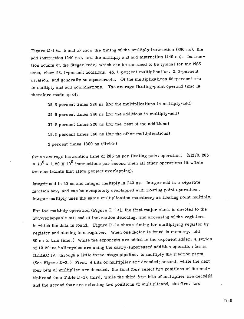
Figure D-l (a, b and c) show the timing of the multiply instruction (380 ns), the

add instruction (240 ns), and the multiply and add instruction (440 ns). Instruc

tion counts on the Steger code, which can be assumed to be typical for the NSS

uses, show 53. 1-percent additions, 45. 1-percent multiplication, 2.0-percent

division, and generally no squareroots. Of the multiplications 56-percent ate

in multiply and add combinations. The average floating-point operand time is

therefore made up of:

25. 6 percent times 220 ns (for the multiplications in multiply-add)

25. 6 percent times 240 ns (for the additions in multiply-add)

27. 5 percent times 220 ns (for the rest of the additions)

19. 5 percent times 360 ns (for the other multiplications)

2 percent times 1800 ns (divide)

for an average instruction time of 285 ns per floating point operation. (512 /0. 285

X 106 = 1. 80 X 109 instructions per second when all other operations fit within

the constraints that allow perfect overlapping).

ns and integer multiply is 240 ns. Integer add is a separate,Integer add is 40

function box, and can be completely overlapped with floating point operations.

Integer multiply uses the same multiplication machinery as floating point multiply.

For the multiply operation (Figure D-la), the first major clock is devoted to the

nonoverlappable tail end of instruction decoding, and accessing of the registers

in which the data is found. Figure D-1a shows timing for multiplying register by

register and storing in a register. When one factor is found in memory, add

80 ns to this time. ) While the exponents are added in the exponent adder, a series

of 12 20-ns half -cycles are using the carry-suppressed addition operation (as in

ILLIAC IV, through a little three-stage pipeline, to multiply the fraction parts.

(See Figure D-2. ) First, 4 bits of multiplier are decoded; second, while the next

the first four select two positions of the mulfour bits of multiplier are decoded,

tiplicand (see Table D-1); third, while the third four bits of multiplier are decoded

and the second four are selecting two positions of multiplicand, the first two

D-5

U 0b

MAJORCLOCK START

-14O'tk- I I I. I I I I

FINAL INSTRUCTION DECODE,

ENABLE REGISTERS INTO A.IJ.

EXPONENT ADD

MULTIPLIER DECODE (10 NIBBLES)

MULTIPLICAND SELECT

CARRY-SAVE ADD

PROPAGATE CARRIES I

2

I

3 1 1i S7

234267991

I 13 4 1 7 I

320ns (IFNO NORMALIZATION)

360n

NORMALIZE

a. Floating Point Multipls'

ENABLE REGISTERS INTO A.U.

SUBTRACT EXPONENTS ALIGN

ADD FRACTION PART

NORMALIZE

•ROUND

I I

t

t

A

I

I 240"s 240

Y

ADD 40n FORRENORMALIZATION IF NEEDED(AFIo0, Nev,)

b. Floating Point Add

ENABLE REGISTERS INTO A.U.

EXPONENT SUBTRACT/ADD

MULTIPLIER DECODE

MULTIPLICAAND SELECT

CARRY-SAVE ADD

PROPAGATE CARRIES

ALIGN

AD

NORMALIZE

ROUND

I

I

FOR MULT.I FORALIGNMENT

I 2 3 4 * * 440,1s

ADD40ns FOR RENORMALIZATION -n IF NEEDED

c. Floating Poinb Multiply Add

Figure D-1. Instruction Timing

ISLUjbItK OUb

CARRY

(1FF)

MULTIPLICAND I ITS MULTIPLIER (39 BITS) (39 BITS)

MULTIPLIER DECODE 20 NS

1 (20 NS)

DECODED

CULTIPL IER

SELECT +1, -1, +2,

MIULT I PL ICAND SELECT (2 tS) LATCHES >

CSA2' NO ADDERS]CARRY-SAVE

Cn+ L TRUE IF 2 of an, bn, c , TRUE

Sn TRUE IF an, b , Cn I OR 3 TRUE

"-I (20 [IS)

(20 NS) CA N.1

A~UNRESOLVED - uPARTIAL

(39 + GUARD BITS) (39 + GUARD BITS)

Figure D-2. Multiply Logic

D-'

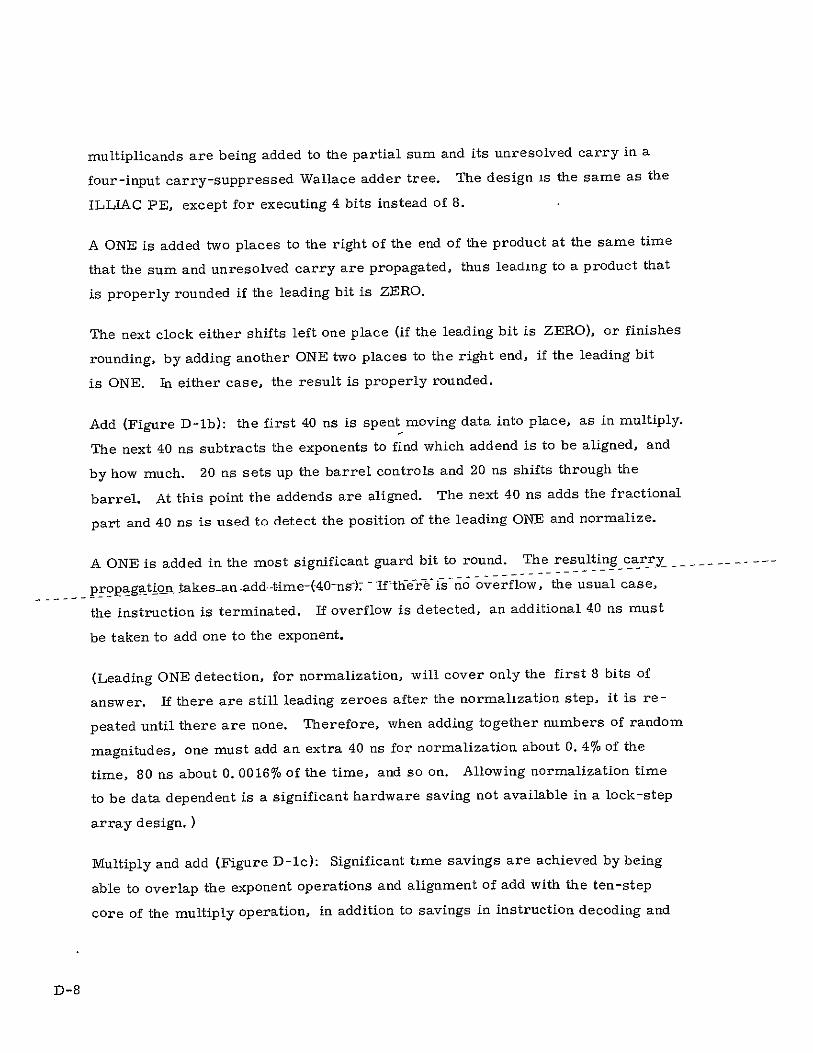
multiplicands are being added to the partial sum and its unresolved carry in a

four-input carry-suppressed Wallace adder tree. The design is the same as the

ILLIAC PE, except for executing 4 bits instead of S.

A ONE is added two places to the right of the end of the product at the same time

that the sum and unresolved carry are propagated, thus leading to a product that

is properly rounded if the leading bit is ZERO.

The next clock either shifts left one place (if the leading bit is ZERO), or finishes

to the right end, if the leading bitrounding, by adding another ONE two places

is ONE. In either case, the result is properly rounded.

ns is spent moving data into place, as in multiply.Add (Figure D-lb): the first 40

to find which addend is to be aligned, andThe next 40 ns subtracts the exponents

by how much. 20 ns sets up the barrel controls and 20 ns shifts through the

are aligned. The next 40 ns adds the fractionalbarrel. At this point the addends

used to detect the position of the leading ONE and normalize.part and 40 ns is

-A ONE is added in the most significant guard bit to round. The resulting carry ....

propagation takes-an -add--time-(40-ns-). - 'Ifth-e-is-no overflow, the usual case,

If overflow is detected, an additional 40 ns mustthe instruction is terminated.

be taken to add one to the exponent.

(Leading ONE detection, for normalization, will cover only the first 8 bits of

answer. If there are still leading zeroes after the normalization step, it is re

peated until there are none. Therefore, when adding together numbers of random

magnitudes, one must add an extra 40 ns for normalization about 0. 4% of the

time, 80 ns about 0. 0016o% of the time, and so on. Allowing normalization time

to be data dependent is a significant hardware saving not available in a lock-step

array design. )

Multiply and add (Figure D-lc): Significant time savings are achieved by being

able to overlap the exponent operations and alignment of add with the ten-step

of the multiply operation, in addition to savings in instruction decoding andcore

D-8

since aregister manipulation. Also, normalization after multiply is omitted,

than one binary place. Also, roundproduct can never be unnormalized by more

can be saved and entereding of the product is omitted since all the guard bits

into the addition step, giving better precision than rounding and saving time.

Normalization of the sum is subject to the same comments made under the des

cription of the addition operation.

Skipping over strings of I Is would apparently allow more than 4 bits of multiplier

to be eaten up per crack. It has been determined that added logic complexity

of data-dependent shift distances makes each "crack" much longer in time. Thus

we choose for the baseline system the algorithm described.

Further explanation of the skipping-over-ONEs multiply algorithm is in the

footnote* for any curious reader.

If the run of ones is of length one, we represent it as a single +1

+1 0000001

and the average length of this sequence is 3.

*It is well known that a string of l's can be represented as +1 in the binary place

at the binary place of the last string. Therefore webefore the string, and a -1

represent most occurrences of a string of one or more zeroes (none or more at

the beginning of the multiplier) followed by a string of two or more ones as such

a +1, -1 pair:

+1 0 0 0 0 0-1

00000111 1 1 1

2, if the bits are random. Therefore the averageThe average length of a run is

guaranteedlength of this sequence is two zeroes, followed by the first ONE that is

to be there, followed by two ONEs.

D-9

The probability of the second bit after the first ONE being one, is 50 percent if

bits are random. Therefore, the average number of bits per crack is

2. 75 bits per crack = 0.5(5/2) + 0.5(3/1)

The leading bit of the multiplier is always 1 (our floating point numbers are always

normalized). Therefore the multiplier can merely be left in place in the double

length partial product accumulator.

D. 3 CLOCK

The logic design of the transposition network, of the interface to the data base

,memory, of the synchronization instruction, and of certain diagnostic tasks, is

made much more feasible if all processors are clocked in synchronism, and if

all extended memory modules are also clocked in synchronism with them. Some

clocks may be deliberately phased differently than others,forn example-the -CU - -..

-clock nfay b6 X-cl6ck cycles ahead of the processor clock (In ILLIAC IV, X is

about 1. 5), but parallel components are clocked simultaneously.

Clock distribution involves a fanout tree from a single clock source. The clock

source is contained within the diagnostic controller, since it is there that single

clocks, or bursts of N clocks, would be generated. An analysis of delay tolerances

will be needed in order to determine whether, for maximum clock rate, it will

be necessary to insert clock timing adjustments into the tree. These adjustments

are included in ILLIAC; but in 1972 it appeared that the machine would have done

as well without them.

When two digital machines of incommensurate clock rates interface, there is a

subtle and disastrous (because it is hard to debug) problem that may arise called

the asynchronous to synchronous conversion problem. The probability of losing

D-10

a bit at such an interface can be designed to be as low as desired (for example,

one bit in 10 100), but cannot be made zero. Without'proper design, errors such

as a control bit being percieved as a ONE in some place and as a ZERO in

another will arise, too often to be tolerable, but too infrequently to be found by

normal means.

Variable clock frequency is included both to allow marginal checking, and as a

tool to help find asynchronous to synchronous conversion problems.

The clock generator shares any uninterruptable power supply that may be needed

in the DBM or the EM. If these items need uninterruptable power, than, of

power failure in the rest of the equipment must be sensed and transmittedcourse,

to the controls of the DBM and EM in order for them to protect whatever informa

tion they contain.

on, supplied to the diagnosticUnconditional clock, emitted whenever power is is

Memory cycles are emitted by concontroller itself, as well as to DBM and EM.

trols contained within the CU, and hence it is not necessary to suppress clocks

to suppress operation in memories. Furthermore, memory cycles should be

completed when initiated.

on front panel switch settings)Conditional clock (conditional on DC command or

Figure D-3 shows a simplifiedis transmitted to the rest of the equipment.

diagram of the clock distribution network.

D. 4 ERROR CORRECTION AND DETECTION LOGIC

Two subjects come under this heading:

1. Generating the corrections and detections for the error control

codes in memory.

2. Generating the check digits for the modulo-n check on arithmetic ope rations.

D-1l

- - ---- ---- --

------------------------

D. C. INPUTS FOR CONTROL i FREQUENICY CONTROL (MIANUAL)

CLOCK N-CYCLE

GENERATOR COUNTER (IN DIAGNOSTIC

CONTROLLER)

TO DC

UNCONDITIONAL TO DBM (TRU CONTROLLED-LENGTH CABLE

CLOCK TO Eli BAYS

9 (THRU CONTROLLED-LENGTH CABLE)

TO CU

CONDITIONAL ON DC

TO BAY FANOUT BOARDS, THRU EQUI-LENGTH CABLE

---------------- AOT-BAD---------------------ZA

EQUI-LENGTH CABLES TO ROW FANOUT BOARD

RWFANOUT BOARD

EQUI-LENGTH CABLES TO PROCESSORS

PROCESSOR INTERFACE

[l l CLOCK RECEIVER

(PER PROCESSOR)

FigureD-3. Clock Distribution

D-12

The data sheets on the Motorols MCI016S/MC10193 circuits give a thorough and

comprehensive discussion of the parity generators required for a Hamming plus

parity single error correcting, double error detection code. Figure D-4 shows

the parity checking pattern of these two chips. Compared to the Motorola pattern,

in Figure D-4, is the pattern of checking parity in the code for 48 data bits, when

the parity and Hamming check bits are inserted into the proper locations. With

or fetched from thethe bits thus ordered, one MC 10163 is needed for data sent to,

transposition network.

A problem is the incompatibility in d-c levels between MECL 10k and Fairchild

100k. Although the levels nominally match, in fact, they track differently with

temperature, and there is much loss of noise margin if 10k and 100k are connected

together. Also, the 12 or i3 exclusive-OR gate density of these chips is not the

LSI density need to implement the NSS within the space, wire-length, and power

budget set.

Motorola, in discussing the use of these chips for parallel-word error detection,

says that they can detect the error in 20 ns, and correct it, provided that comple

menting flip-flops are used for storing the data. The complementing flip-flop

represents a substantial investment in delay compared to a simple latch. The

20ns makes no allowance for wiring delay, or for the delays through any gates

needed for control. It is a lower bound only.

For checking arithmetic as suggested in section 2. 8, checks using arithmetic

modulo 15 or modulo 3 are prime candidates. Modulo fifteen fits the likely size

(four or eight bits wide) of bit-slice arithmetic units. However, there is no known

method for generating the casting-out-fifteens check that does not require hardware

whose complexity is on the order of magnitude of an adder, of the same general

speed as the adder of the PE, if it is to keep up with it.

a somewhat simpler logic implementationFor casting out 3's, on the other hand,

Since five ninths ofis available. Casting out 3's is a weak check in one sense.

all products equal zero, if errors occurred at random, many multiplications will

D-13

EYTF "

TYTE NO.MC 10163 BITBIT 1 2 3 4 5 1 2 3 4 5 6

OUTPUT

0 x PARITY BIT X

I X x IST CHECK BIT X X

2 x x 2N1D CHECK BIT X x

R 0 xx X 3RD CHECK BIT x x

- 4 x x

5 x x x 1 x x x 6 x x x 2 x x x

7X X X X 3 x x x x

4TH CHECK BIT x x

MC 10193 4 x x x

OUTPUT 5 X X X

1 2 3 4 5 6 X X X x 6TH 7 X X X

0x 8 x x.

----------- -x------------ 9 x x x x

2 X X X 10 X X X X x

3 X x x 5TH CHECK BIT x x 4 x xx 11 x x x 5 X x x 12 x x x 6 x x x 13 X X X X 5TH

7X X X X X X X X

X X. X

etc.

Figure D-4. Parity Check Patterns

D-14

go unchecked. However, any error corresponding To a single-mDi errur i eiLii "

input operand or in the result will be checked. This does not include all single

signal faults in the logic.

The discussion is arranged in two parts. First, a disclosure of the general method

of generating the check digits modulo b-i, and second, a specific logic design,

case.somewhat simpler than an adder for the modulo 3

C. 4. 1 General Method

An algorithm for generating the value of an arithmetic number modulo 15 (15 is

taken as an example only for the sake of being specific, it makes the argument

easier to follow) is as follows. Mark off the bits in groups of four. Optionally,

delete any that are "1111". Add the rest. Repeat this process until there are

only four bits in, the result, which will then be the value of the original number

modulo 15. Alternatively, each group of four can be added sequentially with end

around carry and special care of lllls. Figure D-5 and Figure D-6 are block

diagrams of the logic that might implement the processes shown in Table D-2

(a and b). Table D-2b is a.method of Rao.

Method (a) can be implemented by a tree of adders most of them four bits wide,

like the Wallace tree for multiplication, as in Figure D-5. For an 80-bit wide

original number, the process may iterate as many as three times, so the tree

could be used recursively for three clocks, or three trees could be stacked (the

last one having only a single one of the 4-bits wide adders in it. The adder

inputs are various widths, as shown on the diagram' If all the adders were

stacked end to end to' make a single 2-input adder, it would be 94 bits wide,

somewhat longer than the 80-bit original word length.

Method (b) could be used to convert the word slowly into the check digit, with

one 4-bit adder repeatedly used for 20 clock times, but the NSS can not stand

such a trade of time for hardware. All 19 4-bit adders would make an adder 76

bit wide.at reasonable speed. Therefore, a quantity of hardware is implied

equivalent to an adder as wide as the word whose check bit is to be calculated.

D-15

fIXVALUE 280) I I FIRST TOTAL

+ BITS UIDE)

55 BTS WIDE

-- SECONID TOTAL

I BIT IIDF AS . . .. . . .. . . . . . . . .

- - -- - - --- - - - -.-ADDER -BUT-. . . . . . . . . . . . . ... . . . ... .. -- ... . . . . ... . "1I-BIT CARRY

4 BIT RESULT THIRD

TOTAL

Figure D-5. Forming Check Digit by Tree of Adders (Max. Delay 7 Adders)

B-STCHECK DIGIT

Figure D-6. Check Digit Formed by Using Chain of Adders, with

Sum Rippling Through Chain

D-16

Table D-2. Check Digit Schemes

a. Adding in Parallel

10110111000111111011001100101001000010011001010110000ooo 1011 OR 1011 0111 0111

Original binary qurnter 0001 Cast 0001 .... Out 1111 Not Casting 1011 15 1011 0011 0011

Added by groups of 0010 0010 four casting out any 1001 1001

"1111"s 0000 0000 1001 1001 1001 1001

0101 0101 1000 1000 0100 1l1

Ist Total 01001111 01011110 1st Total

Recursion . 0101 1110

Second Total 0100 10011 Second Total

0011

0100 Third Total

b. Adding Sequentially

10110111000111111011001100101001000010011001010110000100 1011 0111

0001 -100

1011

0011 0011

0010 0101 1001 1110

0000

TlO 1001 1000

1001 0010

0101 0111

1000 1111

0100 0100

D-17

I QA y

D I

wi

I.I

Figure D-7. Logic Block for Modulo Three Check-Bit Generator (Replaces One-Bit Adder)

-----w--1-------------

FROM NUMBER TO OF AA1 CHECKED D ABB (SEESE

C FIGURE D-7) MOST SIG. BIT D

MOD 3 RESULT I B (SEE

FROM PREVIOUS C FIGURE D 7) LEAST SIG. BIT ADDER C D

D

Figure D-8. One Digit's Worth of Module 3-Check Digit Generator

D-18

D. 4.2 Modulo 3 Case

When the base is 3, we can simplify the adder (now two bits wide) to two copies

of the logic whose diagram is shown in Figure D-7. The output, Q, is given by

X OR Y OR Z OR W.

Table D-3 shows the truth table for the modulo 3 2-bit adder where one input is

two of the binary bits from the number being checked, and the other two are

limited to 00, 01, or 10 (that is, they are the output of another modulo 3 2-bit

adder). Figure D-8 shows the connection of two of the circuits of Figure D-7

to produce one modulo 3 result from two bits of the number being checked, plus

one modulo three input. Table D-4 shows the complete truth table, including

the outputs actually generated for the don't care cases.

Table D-3 Table D-4 Desired Output Actual Output In Out In Out

ABCD ML ABCD ML

0000 00 0000 00 0001 01 0001 01 0010 10 0010 I0 0011 00 0011 00 0100 01 0100 01 0101 10 0101 10 0110 00 0110 00

- 0111 01 0111 01 1000 10 1000 10 1001 00 1001 00 1010 01 1010 01 1011 10 1011 10

llxx xx 11001101 1101

11 10 10 Don't Care Cases.

1110 01 x = don't -care 1111 11

D-19

For comparison with Figure D-7, Figure D-9 shows the normal 1-bit adder.

Figure D-7 is seen to represent 60 percent as much logic as this complete

adder, so we can say that generating the check digit modulo 3 takes 60 percent

as much logic as a full adder would.

CARRY

IN OUT

-I N. N-

. . . .

CARRY OUT

Figure D-9. A Conventional 1-Bit Adder

D-20

APPENDIX E

PROCESSING ELEMENT OF EXISTING COMPONENTS

E. 1 INTRODUCTION

The free-standing processor of the baseline system may have significant applica

tion outside the NSS. Burroughs therefore undertook to investigate the feasibility

of the proposed design by initiating a detailed logic design of major portions of

the processing element, including the integer unit and the floating point unit, and

by making estimates of the parts count of certain other portions of the processing

element, such as the instruction decoding. The ground rule for this work was that

commercially available circuits would be used. Specifically, the parts selected

were members of the Fairchild "l00K" ECL series, which includes a significant

number of complex parts.

Design goals were to minimize the quantity of circuitry without seriously compro

mising on speed. The implementation of the processing element as suggested in

Chapter 3 of Volume I, and in Appendix D, was taken as a guide in specifying the

level of performndce required. Alternate implementations, which accomplish the

same function at comparable speed, are sometimes required to reduce the parts

count when using commercially available parts.

Ei

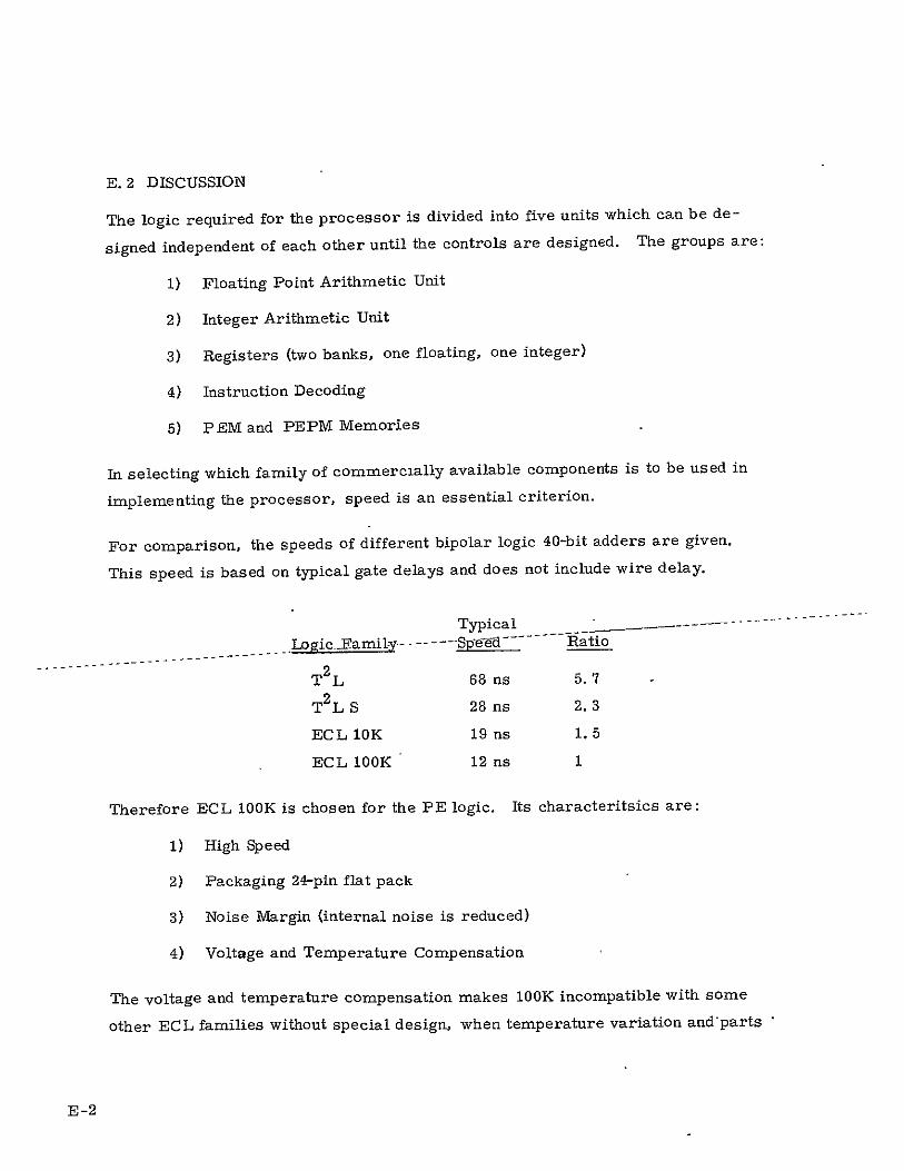
E. 2 DISCUSSION

The logic required for the processor is divided into five units which can be de-

The groups are:signed independent of each other until the controls are designed.

1) Floating Point Arithmetic Unit

2) Integer Arithmetic Unit

3) Registers (two banks, one floating, one integer)

4) Instruction Decoding

5) PEM and PEPM Memories

In selecting which family of commercially available components is to be used in

speed is an essential criterion.implementing the processor,

areFor comparison, the speeds of different bipolar logic 40-bit adders given.

This speed is based on typical gate delays and does not include wire delay.

---. -------Typical

LOgic-Eamil-y-- ---- Se-d ...------- Ratio

T2L 68 ns 5.7

T2L S 28 ns 2.3

ECL 10K 19 ns 1. 5

ECL 100K 12 ns 1

Its characteritsics are:Therefore ECL 100K is chosen for the PE logic.

1) High Speed

2) Packaging 24-pin flat pack

3) Noise Margin (internal noise is reduced)

4) Voltage and Temperature Compensation

some

other ECL families without special design, when temperature variation and'parts

The voltage and temperature compensation makes 100K incompatible with

E-2

tolerances are taken into account. Thus, the choice of ECL lOOK introduces a

restriction, but as Table B-i shows, there is a large well-chosen repertoire of

parts available.

E. 3 LOGIC IMPLIEMENTATION

E. 3. 1 Floating Point Arithmetic Unit

E. 3. 1 1 Shifting

Shifting is required for alignment and for normalization. A full barrel switch

would require 40 chips at about 25 ns circuit delay. When a shift register is used

(this can also be used as a register), the speed is a function of the number of bits

to be shifted, since most shifts are over short distances, and data-dependent

timing is allowed. This would require 6 chips at a speed of 2.7 ns min. , 65 ns

max. and typical 22 ns. When the same shifter is used with minimum logic it

would require 9 chips and a maximum delay of 25 ns.

Alignment requires 2 chips and 10 ns plus shifting 2. 7 ns /bit.

Normalization requires 1 dhip and 10 ns plus shifting.

E. 3. 1. 2 Multiplication

Multiplier chips were considered and rejected. It would require 25 8 by 8 multi

plier and 35 adder chips for a total of 60 chips and at a speed of 210 ns, or ten

12 by 12 multipliers and 20. adder chips for a total of 30 chips at a speed of 200 ns.

The adder member of the family (100180) can be used at a speed of about 14ns per

40-bit addition. By having three times the multiplicand stored in a register, two

bits of multiplier can be used up per 14 ns adder cycle, giving the "core" of the

multiplication running ir" 280 ns (20 iterations of 14 ns each as compared to 240ns,

10 iterations of 20 ns each plus 40 ns carry propagation as described in Appendix D).

This multiply is only slightly slower than that found in the baseline system.

E-3

shift register fbr accumulating theThe s-elected implementation therefore uses

partial product, and standard adder with two bits of multiplier per addition. This

requires 9 chips, and takes 280 ns not including set up. The multiplier chip im

plementation appears faster on the surface, however the larger number of chips

so the actual speeds may be comparable for theimplies greater wiring delays,

speed of 10 ns.two systems. The exponent logic requires three circuits at a

E. 3. 1. 3 Floating Point Registers

Sixteen floating point registers are assumed.

E. 3. 2 Integer Arithmetic Unit

This performs address calculation using 16 -bit integers and calculations on

double-length 32-bit integers.

A single-length adder is proposed, with two adder cycles being used for the 32

bit additions. The parts count assumes a one-bit of multiplier is used to control

one adder cycle, so that multiplying two single-length integers takes sixteen adder

.. cycles,_ and-multiplying a-3-2-bit-inte-gei by- 16-bit integer takes 32-add cycles.

A shifter in the integer unit is used not only for the multiply function, but also

for the shift instruction, used in conjunction with the test bit instruction for bit

vector-control of the processor.

The same adder, and lookahead chips are used as in the floating point unit.

Sixteen 16-bit integer registers were assumed.

E. 3. 3 Instruction Decoding

Instruction decoding is assumed to be done with read-only memory and a micro

coded version of the instruction description. The number of words and bits per

word in the microprogram memory are estimated based on past experience with

other processors of comparable complexity.

E-4

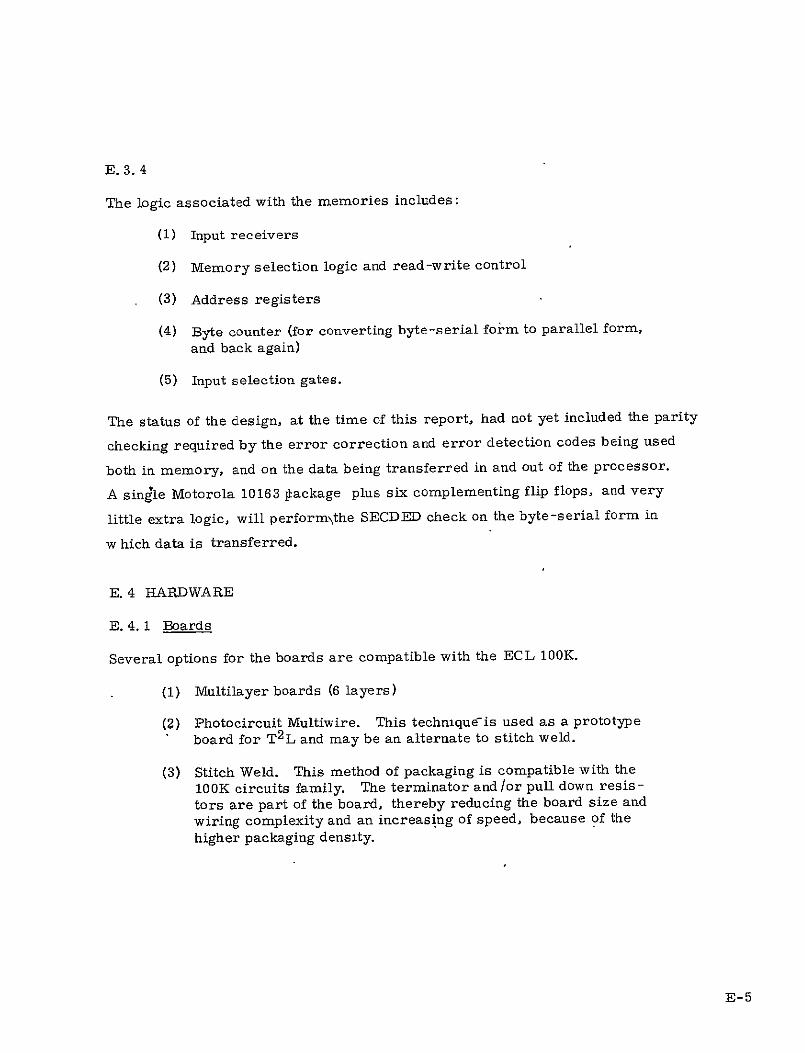
E. 3.4

The logic associated with the memories includes:

(1) Input receivers

(2) Memory selection logic and read-write control

(3) Address registers

(4) Byte counter (for converting byte-serial foim to parallel form,

and back again)

(5) Input selection gates.

The status of the design, at the time of this report, had not yet included the parity

checking required by the error correction and error detection codes being used

both in memory, and on the data being transferred in and out of the processor.

A single Motorola 10163 4ackage plus six complementing flip flops, and very

little extra logic, will perform\the SECDED check on the byte-serial form in

w hich data is transferred.

E. 4 HARDWARE

E. 4. 1 Boards

Several options for the boards are compatible with the ECL 100K.

(1) Multilayer boards (6 layers)

(2) Photocircuit Multiwire. This technique-is used as a prototype board for T 2 L and may be an alternate to stitch weld.

(3) Stitch Weld. This method of packaging is compatible with the

100K circuits family. The terminator and/or pull down resis

tors are part of the board, thereby reducing the board size and

wiring complexity and an increasing of speed, because of the higher packaging density.

E-5

Table E-1. Processor Parts Count,

Functional Unit

Floating Point Arithmetic

8 x 100180 3 x 100179 2 x 100136

10 x 100141 4 x 100163

Integer

3 x 100180 1 x 100179 2 x 100141 2 x 100136 6 x 100171

Registers

18 x 100145

Instruction DECODE

36 x 100416

Instruction Selection

10 x 100171

Memory Control*

2 x 100141 4 x 100136 6 x 100171

ADDER LOOKAHEAD COUNTER SHIFTER SELECTOR

ADDER LOOKAHEAD SHIFTER COUNTER MULTIPLEXOR

Register File

Memory

Selector

SHIFTER COUNTER Multiplexor

6 x differential receiver

Miscellaneous

Control

Driver, etc.

*Memory chips proper not included

if Built of ECL 100K

No. of Chips

27

14

18

36

10

18

17

Total 140

E-6

E. 4. 2 Processor Module

The design assumes that each PE is a free standing module with its own power

supply and clock. This is favorable because of the relatively low number of

interconnections (50 - 80).

E. 5 SUMMARY

Table E-1 summarizes the parts used in this effort by type within each of the

functional units. Not included in this table are the parity checking logic needed

for error detection and correction Furthermore, a detailed design of the control

logic has not yet been carried out. An estimate of 17 packages is included to

cover control, clock and fanout but not parities.

E-7

APPENDIX F

A TRADEOFF STUDY ON THE NUMBER OF PROCESSORS

This appendix describes the technique for optimizing power per processor versus

number of processors from the viewpoint of cost. If processors are to be run in

parallel on the block tridiagonal code by all marching on a plane front through the

grid in parallel, temporary storage is required on the order of 75 temporary

variables times the length of the dimension along which the computation-is going,

times the area (in number of grid points) covered by the plane front. Figure F-I

illustrates this situation. The problem addressed here is that of finding the

relationship between number of processors, amount of memory, and cost of the

Navier-Stokes solver, due to this temporary storage requirement.

F. 1. ASSUMPTIONS

The computational grid will be assumed to have N3 points. The results will not

differ -much if the grid in fact has somewhat different lengths in the two dimensions.

The cross section of the pencil will use all P processors to compute M2 grid points.

The assumption of a square pencil will matter somewhat, if the sides of the pencil

cost extra computation, and the square shape minimizing that extra cost.

C aM2 F

F-i

PENCIL LENGTH EXTENDS FROM END-TO-END ON ONE DIMENSION. CROSS SECTION IS A PLANE OF M2 POINTS

SPACE COVERED

GRID

/ h M~i, PLANE IN \WHICHt Y C COOTPUTAT I

OCCURS, WI\LL"N

~ONE SWEEPENDPENCILTO T14EFROM

OTHER AND BACK

Figure F-i. Computational Grid with Plane of Computation Proceeding

Through Pencil

F-2

where a represents the work done per grid point, including the fetching from ex

tended memory. The constant C has been estimated at one billion floating opera

tions per second.

The speed of the individual processor is C 0 /P (there are P processors). Define

Co/P as Cp.

To the rather elementary level of approximation used here, it may also be assumed

that the speed of memory Sins defined as the reciprocal of access time, is also

proportional to computational speed, or:

S cc m p

where c is the constant of proportionality.

The total amount of main memory is equal to that part of the data base that can be

divided among the processors, (a constant), plus the working storage, (pro

portional to the number of processors), plus the program store (also proportional

to PE's, since every processor has its own copy of the program). Thus:

M = e+fP+pP

e = the per processor constant

f = 75N (the temporary storage requirement previously mentioned)

p = 8, 000 (the program storage)

where f is slightly larger than 75N because of other temporaries, but is surely

dominated by the 75N term. A program store of 8, 000 words is plausibly assumed.

M = 4,000 + (9, 000 + 75N)P

is the total memory requirement, (not counting extended memory).

Total cost, H, is memory cost plus processor cost:

H = H +H m p

F-3

- - - ----------------------------------- ------------- ---- ---------

UNACCEPTABLE COST j HS (MEMORY

COST PER WORD)

Sm (SPEED OF MEMORY)

Figure F-2. Memory Cost Per Bit. vs. Speed

F-4

Memory cost Is a function of amount of memory and speed of memory. It can be.

factored (approximately, assuming that the total memory is larger than any con

straints imposed by optimum module size):

HIn= M-K s(S , M/P)

where H is the cost per word as a function of speed and module size. 5

Processor cost is a function of speed

H = PHc(C) p c p

H c is the cost of the individual processor, written as Hc(C p ) to emphasize its

dependence on processor speed.

F. 2 DISCUSSION

The memory cost function exhibits discontinuities. For example, the fastest mem

ory that can be built with 16k-bit chips may be on the order of 100 ns. More speed

imposes sharply increased costs, at least in part to overcome the unreliability

imposed by a too large chip count if small (4k-bit) chips must be used.

Figure F-2 shows the situation as it might be. It is expected that any memory

speed faster than that available in 16k-bit chips will have unacceptable cost, and

puts a firm constraint on the design.

It is also expected that between breaks on the curve, H is fairly flat. HI is

therefore dominated by a term proportioned to P, over a range.

The cost of the individual processor, H c , is a little hard to estimate. For the sake

of carrying the analytic approach further, assume for small processors, '(where

design is straight forward) a curve that follows Grosch's Law, and then add to it a 2

term in Cp to express the difficulties encountered in trying to design a faster

processor than is reasonable in the given state of the art,

2 gC 1/2+hCH = p pc

where g and h are constants of proportionality.

F-5

---------------------------- -----------

Combining the equation H = PH and the equation for C givesp c p

Hp = gJECo+ h(Co2 /P)

Solving for optimum H by setting dH /dP = 0, we find p p

P'opt = (2h/g)2/3C

The prime indicates we have optimized only processor costs, ignoring the effect of

memory cost. The presence of out-of-pencil computations will raise the optimum

number of processors slightly.

The above optimum does not take memory into account. Total cost is given by:

H = H +H m p

= MH +PH s C

= (400 + (16000 + 75N)P)H +-+-h -0- -- E-

Arguing that the optimum will be influenced only weakly by the second term, since

there is so much memory in the system, the optimized total cost H becomes a

simple function of P, and over any range where Hs is essentially constant:

P .= C h or (16000 + 75N)H s = hC 2 opt- o \(16000 + 75N) Hs p

Numerically, this is not very precise, since there is difficulty in quantifying h, a

constant representing the increased difficulty of designing very fast processing elements. Note that at optimum, the marginal cost of the additional memory for

another processor is equal to the extra processor cost incurred by having one fewer processor. This solution is only valid over a limited range of memory

speed Sm. If Pop corresponds to a faster or slower S than allowable, than the actual optimum will be at the end of the range.

F-6

F. 3 OPTIMIZATION

The optimum processor design is apparently right at the breakpoint on the mem

ory cost curve, namely where 16K-bit memory chips are used at their fastest cycle

time. If memory is 100 ns cycle, then this upper limit is a few (maybe three)

M flops, since every flop requires not only one to two operands to be fetched but

also index values and instructions. A 3-Mflop PE, set into a 1-gigaflop require

ment, results in 512 PE's (if 75 percent efficiency is allowed). Separate program

and data memories are indicated.

One might think that faster memory could be achieved by interlacing memory.

Beyond separating program and data, this requires that the processor be arranged

as a vector processor, and the result is that the work within each and every PE

must be arranged in vector form, over and above any vectorization or equivalent

parallelization that was applied to permit the array type parallelism in the first

place. Such two-way vectorization is not covered by this analysis, and may well

call for even more total memory than that assumed here.

F. 4 MEMORY REQUIREMENTS

Given assumptions stated above the total amount of memory as a function of the

number of processors can be estimated. For comparison purposes, assume

total memory is the sum of:

(1) 15, 000, 000 words of aerodynamic data base information

(2) 7500P words of temporary storage, +4000? words of other data in PEM.

(3) 8000P words of program store.

(4) Other increments that are probably negligible by comparisdn.

F-7

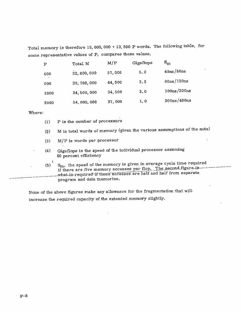
15, 000, 000 + 19, 500 P words. The following table, forTotal memory is therefore

some representative values of P, compares these values.

P Total M M/P Gigaflops Sm

400 22,800,000 57,000 5.0 4Ons/80ns

600 26,700,000 44,500 3.3 60ns/120ns

1000 34,500,000 34,500 2.0 lOOns/200ns

2000 54,000, 000 27, 000 1.0 200ns/400ns

Where:

(1) P is the number of processors

total words of memory (given the various assumptions of the note)(2) M is

(3) M/P is words, per processor

(4) Gigaflops is the speed of the individual processor assuming

50 percent efficiency

(5) Sm , the speed of the memory is given in average cycle time required

are five memory accesses per flop.-Thesec~ond-figur-is ------if there e-acegssa-rehalf and half from separate

- - .... what-is--required-if-ths program and data memories.

None of the above figures make any allowance for the fragmentation that will

increase the required capacity of the extended memory slightly.

F-8

APPENDIX G

HOST SYSTEM

G. 1 OVERVIEW

The Numerical Aerodynamic Simulation Facility is specifically dedicated to

aerodynamic simulations using the Navier-Stokes Solver. The NSS is thus the chief

ingredient of the NASF. However, the NSS is specialized to its particular task;

since there is no need to design custom equipment to perform those supporting

functions for which commercially available equipment can be bought.

A block diagram of the system, including NSS, was given in Volume I. The entire

system in addition to the NSS including its Data Base Memory, consists of a host

processor, whose functions are enumerated in the next section, a file memory for

which disk packs have been selected, some rather normal peripherals, an archive

memory to hold 2 X 1012 bits of information, and interfaces to the interactive users.

Figure G-1 shows some of the transfer paths in this system. The transfer rate

between DBM and the rest of NSS is 140 X 106 bits per second including error con

trol about 120 X 106 bits per second of actual data. The transfer rate of typical

disk packs is about 107 bits per second per channel.

From the point of view of the software, the NSS is an adjunct to the host processor,

which is the element with which the users interface.

,.I 0-1 7

IISS

DBM

6,667 WORDS/SEC AVERAGE RATE

USERS HOST 2 CHANNELS (I REQUIRED) AT i07 BITS/SEC. 3 PERCENT LOADING

PERILHERALS - . . . . . . . . . .

PRINTERS, DISPLAYS

DIS PACKS

FIXED BY ARCHIVE

DESIGN

ARCHIVE

Figure G-1. System Transfer Paths

G-2

Archive, disk packs, and DBlM are all attached as peripherals of the host pro

cessor, as that is the architecture supported by commercially available hosts.

Figure G-1 shows data transfers being made directly; functionally this is correct,

but in fact this data could be buffered in the host's memory. A good host will not

require these transfers to take any of the host processing power except for the

initiation of the I/O transfers.

The highest transfer rate between DEM and file memory occurs in response to the

requirements of the Table 8-18 in Chpater 8, where item 313 shows an average

of 6667 words per second being unloaded into DBM. These words are destined

for processing in the host, either concurrently, or after a time of residence in

the file system. Restart dumps and loads (items 1. B and 2. A of Table 8-18), are

5 X 10 words every 10 minutes. Allowing for traffic both out and in, this comes

to an average of 16, 667 words per second, or just under one million bits per

second. Some fraction of this traffic is backed out from DEM to disk packs in the

file system. For a worst-case analysis, we can assume all of it is, for a total

average transfer rate of 23, 333 words per second or 1. 28 million bits per second.

In transferring to and from packs, block sizes are large, so whole pack tracks

could be transferred as a single block at the 10 MHz transfer rates expected of disk

packs in the 1980 time frame. The entire 1. 28 million bits per second is only

12. 8 percent of the capacity of a single channel. The baseline system has two data

channels from DBM to the host. Clearly, such duplexing is for reliability reasons,

not because of transfer rate requirements. This statement applies only to the

benchmark programs. Other applications may well require higher bandwidth at

this point. Such higher bandwidth would be easy to supply.

G. 2 HOST PROCESSOR

The host processor contains the chief portion of the operating system, interfaces

with users, and handles the file system. Its functions are:

(1) Compiling for the NSS

(2) Scheduling for the NSS

(3) File system

(4) User interaction, remote users and local graphics users

G-3

(5) Debugging aids for the NSS

(6) Confidence and Diagnostic checks on the NSS

(7) I/O formatting

(8) Linking of NSS programs

(9) Grid generation and modification (insofar as this is not run on

the NSS). A user-written program.

(10) Body geometry generation and modification.

(11) Grid and body geometry display.

(12) Data reduction and display.

(13) Standard peripherals.

(14) Loading jobs into the NSS, unloading jobs from the NSS.

(15) Interaction with NSS-resident part of operating system.

Because of the hosts 's central location in the system, it must have a much higher

say 97 percent.availability than the 90 percent required for the total system,

To obtain this level of reliability, some sort of redundancy, or fail-soft mechanism

To this end a Burroughs B 7800 dual-processor iswill be required of the host.

number of distinct advantages:being recommended as host. This system has a

------- (1) Dual-processors--and-modu-lar merorygiVbete -than duplex

redundancy without doubling memory requirements.

(2) The FORTRAN compiler for the BSP, which already contains many

of the features needed-for the NSS compiler, runs on the B 7800.

An opportunity for simplifying compiler development is not to be

ignored.

(3) Languages available for the B 7800 include FORTRAN and ALGOL.

(4) An extensive file handling system, with a significant degree of

security features, comes with the system.

ensures(5) The descriptor mechanism used for accessing memory

that security constraints are not accidentally violated by software

bugs or by hardware faults.

(6) The machine was specifically designed to support interactive users, in a multiprogramming, multiprocessing, virtual memory

mode of operation.

G-4

The major elements of the system being recommended include: two control pro

each with 28 data channels,cessor (8 MHz w/vectors), two input/output processor,

one maintenance diagnostic unit, one operator console with dual displays and con

trols, and two 3, 145, 728 byte memory subsystems.

cover as itMore information on the B 7800 will be furnished under separate

are needed to the B 7800 standardbecomes available. Two or three extensions

softwar% including the operating system MCP (Master Control Program):

Typical archival(1) Inclusion of the archive into the file system. systems appear to the host as a number of disk packs of variable access time. Since the B 7800 already supports disks, the inclusion of an archival system is relatively simple,

provided that attempts to optimize the operation of the archival

system are not made.

(2) Adding the interface to the NSS CU-resident portion of the operating system, and adding the DBM and diagnostic controller as new kinds

of peripheral devices.

(3) Keeping the NSS scheduler and interrupt handler core-resident may not be necessary, since it need be called into use on short

notice only for error aborts. Transfers between DBM and EM are handled by the NSS itself, with no attention from the B 7800

at the time transfers are made. Scheduling can be isolated from

real-time by giving the NSS a queue (which need not be longer than length 2) of jobs to do. If these programs were kept core

resident, it would represent a change from the normal philosophy of the MCP, where virtual memory is an integral part of the operation.

Peripherals to be supplied are a normal-looking lot. They would include:

(1) Card readers (2)

(2) Printers (4)

(3) Tape units (say 12, the exact number depending to the extent that

the archive has to be backed up by tdpe, and to the extent that tape

is used for interfacility transfer of tata) and an MTU exchange.

(4) Disk packs (40 of the highest density available for the file

system)

To this list one must add such user equipments as the remote job entry terminals,

and the graphics display processors, that will be attached to the system.

G-5

Features supplied by standard B 7800 software include:

(1) Compilers, text editors, program libraries to support the user

functions which will be written for the NASF

extension, which will(2) File system (except for the archive

require additional work)

(3) Communications handling for remote users

(4) I/O handling

(5) Virtual memory for user programs running on the B 7800.

G-6

APPENDIX H

ALTERNATE DBM DESIGNS

H. I DISK PACK DBM

Conventional disk packs, with 20 surfaces on each disk, also have 20 moving heads,

one per surface. Each head has a data rate (depending on model) of 5 or 10 Mbits/

sec. Conventionally, one of the 20 heads is selected for the addressing of a single

surface. Nothing prevents one from constructing a customized disk pack in which

all 20 of these heads are operated in parallel, similarly to the 128 heads that are

in parallel on the ILLIAC IV disks. The CDC 819 is a similar storage, with disks

noiremovable.

A cylinder (all the data on one disk pack at a fixed head position) contains approxi

mately 5 X 106 bits. There are 20 tracks of 10 MHz each, theentire cylinder of

5 X 106 bits is written in 25 ms. Since head movement from one cylinder to another

will miss the beginning of the cylinder, apparently two disks, each alternately

writing full cylinders, to keep up with the 140 X 106 bits/sec rate of transfer from

EM, must be used. A double buffer is required for both disks, for a total buffer

memory requirement within the DBM controllers of 4 X (5 X 10 ) bits.

A fairly complex error correction code is used to overcome the existence of

occasional bad spots and reading errors on the disks. One of the burst error

correction codes will be used.

H-I

Todays disk packs hold roughly a 1.4 billion bits apiece. By 1980 we should see

another doubling of density, so that four packs would hold roughly ten billion bits

which would satisfy the NASF needs.

Customizing for parallelism will involve solving a number of design problems that

do not arise on the single channel standard commercial design. These same pro

blems were met head on and solved on the ILLIAC IV parallel head system. They

are:

1. Control of crosstalk between channels during write, including power supply noise induced by the write currents affecting other write currents. Wiring inductances and mutual inductances are critical.

2. Control of crosstalk during read.

3. Additional separation and wiring between head and sense amplifier; there is not room for 20 sense amplifiers in the location used for the single sense amplifier of the conventional disk pack drive.

4. Deskewing. Bit rates of each channel are several thousand bits for each inch of length along the track. If the disks of the pack are elastic enough to move with respect to each other by one or two thousandths of an inch, and they are, then bits that wenewritten ----.----simultaneouslyon -different-trcks fiay-b]e read off those same tracks

----------- mismatched in time by quite a few bit tinies. The deskewing buffers in ILLIAC IV were 3 bits long, and all the heads were on the surfaces of a single disk. Here longer deskewing buffers are expected.

The write drivers, sense amplifiers and logic of a commercially available disk pack

system can not be used without some design modification. A logic rack's worth of

circuitry will be added to each dual disk pack drive.

H. 2 BUBBLES FOR DBM

The one bubble chip currently announced as a product, is TI's MBM 0101. This

chip has 157 shift registers (with not more than 13 of them non-functioning) with

641 bits each. Thus there are 92, 304 storage locations guaranteed good. It is the

controller's responsibility to remember the bad locations in every chip, and avoid

them. Since the access time (4. 0 ms max) is also a function of which shift register

within the chip is selected, parallel operation of chips does not emit data in

parallel, but timing adjustments are required.

H-2

These difficulties make the-TBM 0101 an unattractive chip for constructing

the DBM. Access time is 4.0 ms vs. CCD's few microseconds to the first bit of

the block. Shift rate is 100 kHz versus. 21Mz for the CCD. The package is over

an inch square. TI's tentative data sheet of February 1977 says "the following

interface integrated circuits are required . . . for each MBM" (magnetic bubble

memory chip) "in a system: one function driver, two coil drivers, one diode array,

one R/C network, and one sense amplifier. TheR/C network and sense amplifier

may be shared" with other bubble ships.

In the future, bubble chips should become more self-contained, with these necessary

functions included in the same pabkage with the bubbles. Chapter 5 discusses the

probable availability of suitable bubbles in more detail.

One advantage of bubbles is that error rates should be very good, and so the error

correction scheme should be simple. "Scrubbing" errors is not needed. Errors

created on refresh are less: TI's tentative data sheet on the T]BM 0101 guarantees

3 X 1028 shifts per bit error, a factor of 1012 better than Fairchild's experience

with CCD's.

At shift rates of 100 kHz, it takes a thousand bubble chips operating in parallel

to achieve the desired transfer rate of 108 bits per second. Bubbles, however,

are nonvolatile. Since the bubble chip needed for the DBM has yet to be developed,

it makes little sense to prognosticate there what the design might look like. It is

likely that bubbles even by 1980 will run a poor third in performance, because of

the need for extreme parallelism to achieve the desired transfer rates, and

because of the need to have several outrigger chips associated with each and

every bubble chip.

H-3

APPENDIX I

NUMBER REPRESENTATION

L i INTRODUCTION

Requirements and desiderata for the representation of numbers internal to the

NSS are listed here, followed by a description of the format for representing

numbers that satisfy all the requirements as well as all the desiderata.

Exponen arithmetic shall result in as simple hardware as possible.

Precision shall be predictable independently of exact knowledge of numerical values.

Arithmetic Overflows shall be detectable.

Index Arithmetic is totally separate from floating point operations (the value of an index only occasionally is entered into a floating point expression).

10-digit precision is an absolute minimum.

4-bit or 8-bit bit-slice arithmetic units are available, and are likely to be used in implementing the arithmetic unit.

Different bit-patterns with the same numerical interpretation are to be avoided. Thus, there should not be both a +0 and a -0 exponent.

Sign 8 Bits 39 Bits Bit

Infinity

I± 11111111 undefined

exponent field all ONES

Normal floating point format

± eeeeeeee normalized fraction

Binary Point

Floating point 1. 0 (approximate)

± 10000000 . .. ...... 1111

Floating point 1. 0 (exact)

.000±10000001 100000.. . ........

Infinitesimal

± 00000001 undefined

exponent 1 more than all zeroes

Standard zero

± 00000000 1 00000000 . .... 0000

minimum exponent

Figure I-1. Format

1-2

Rounding arithmetic will be used.

No Interrupts shall be used for out-of-range detection (because of the

highly overlapped, highly concurrent nature of the NSS)

L.2 FORMAT

A floating point format which meets all these criteria is one with a 48-bit word,

first bit sign, next 8 bits exponent in offset format, and the rest fraction.

(Figure I-1).

The largest exponent (11111111) is reserved for "infinity". An exponent overflow

results in the result being set to infinity.

The zero exponent (00000000) is reserved for the representation of zero and as

a prefix for integers when stored in 48-bit words. The standard zero is a word

of 48 ZEROs, that is, a "+" sign, an exponent smaller than the exponent of any

other real number, and an all zero fraction part.

The next-to-smallest exponent (00000001) is reserved for "infinitestimal". It is

programmer's option whether underflow results in zero, or whether underflow

results in infinitesimal. If underflow results in zero, no special test for the

00000001 exponent is made, and it will indeed represent an allowable value of

the exponent.

A binary base for the exponent is preferred.

A rejected alternative is to let all zeroes have the exponent with which they were born, so to speak. If a = 23. 2100, and b = 23. 2100, then a-b would be repre

sented as 0.2100. This tends to suppress meaningless precision, and substitute

zeroes for it. The suppression of meaningless precision, if carred to its logeal

conclusion, will result in something like the precision-preserving mode in ILLIAC IV, as many leading zeroeswhere non normalizing instructions allow one to preserve

in a variable as it is lacking in precision.

I-3

---- ---- -------------------------

1.3 INFINITY, INFINITESIMAL

Infinity and infintesimal are included in the scheme so that arithmetic overflows

can be monitored without the necessity for interrupts, since the NSS has hundreds

of independent operations which are being executed simultaneously.

"Infinity" actually means "undetermined" value. It is called "infinity" because it

will be produced by arithmetic overflow and divide by zero, but uninitialized data

will be set to "minus infinity", with the address in the fraction part.

Infinitesimal is set by exponent underflow. The rules for handling infinities and

infinitesimals entering into arithmetic operations are such that an infinitesimal

can always be reinterpreted as zero.

We choose not to complicate the scheme by having three quantities: "Infinity" for

something known to be unrepresentably large; "infinitesimal" for the unrepresentably

small; and a third code for "unrepresentable of indeterminate magnitude" which

would result from operations such as infinity times infinitesimal.

The exponent field has the following detection applied-to-it: ------- --

* The carry out of the exponent field, and the sign of the exponent, combine to give an overflow/underflow indication.

Exponent field of 11111111 and 00000001 are detected on input operands.*

* An exponent field of 00000000 is also detected coming out of an arithmetic operation, as it may represent an underflow, dependent on what the input operands were.

A set of rules for handling and responding to infinities and infintesimals is:

* Sign logic is independent of overflow, underflow, infinity or

infinitesimal.

* Infinity times anything, including zero, is infinity. Zero is

included since the exponents going into the operation that produced

the zero is not known, and therefore the possible intended value of

the result of such a product is not known.

* Infinity divided by anything is infinity.

i-4

* Infinity plus or minus anything is infinity.

* Anything divided by infinity is infinity.

* Except for zero times infinity, zero times anything else is zero.

* Zero divided by a real number is zero.

* Any number divided by zero is infinity.

* Infinitesimal times a real number or an infinitesimal is infinitesimal.

* Any number divided by infinitesimal is infinity.

* Infinitesimal divided by a real number is infinitesimal.

* Infinitesimal plus or minus a real number is that real number.

* Infinitesimal plus or minus zero or infinitesimal is infinitesimal.

I.4 CHOICE OF EXPONENT

Base. Base 2 is preferred from a predictability of precision point of view, and

is perhaps conceptually simpler.

Base 4, with the same exponent range, takes one less exponent bit, and therefore

allows the representation of one more bit of precision for half the numbers (although

in a long calculation, half the input variables will have a leading zero in the frac

tion part, so that the resulting increase in precision is, on the average, only a

small fraction of a bit. The product of N variables of random values, are on the

average 0. 21 bits more precise in base 4 than in base 2 if the intermediate products

are all double length. )

Base 16, an industry standard, loses a full bit of precision on many numbers and

almost a full bit on a long calculation involving many numbers of random exponents,

compared to base 2. Not all shift distances need to be covered, so the normalization

logic (if done in parallel, with a barrel) is approximately one logic level less.

Example designs show about 3/4 as many gates required in the normalization

network at base 16 compared to base 2.

1-5

- ------------------

Choice. of base is irrelevant to the trick of being able to normalize by a single

shift after the multiplication of two normalized numbers (there dan be only one

leading 0 in the base of the exponent).

Base 2 facilitates special instructions such as "*1/2". It makes the normalization

network identical' to the shift network (if shift instructions are needed).

The desire for predictability of precision makes base 2 weakly preferred, since

there seems to be little else to make us choose between base 4 and base 2.

Format. Exponents can be sign and magnitude, 2's complement, or offset. Sign

and magnitude leads to two different exponents with the same significance

(+0 and -0), and more complex hardware for exponent arithmetic. (By "offset"

exponent, we mean a notation that differs from 2's complement only in the leading

bit, using "I" for positive and "0" for negative instead of vice versa).

Offset notation and 2's complement notation are almost identical, and both are

preferred over sign and magnitude notation for the exponent. InILLIA-G,--offset-------

-- - notation-was-preferrdc e6anseit simplified the logic of comparing two numbers

of the same sign (or comparing magnitude). Starting with the first exponent bit,

that number is larger in magnitude which as a "I" in the first bit location where

the numbers are not equal. This simple rule, true for unsigned binary numbers,

works also for normalized floating point numbers with offset exponents.

Two's complement simplifies (by one gate) the logic required to compare two ex

ponents for alignment prior to adding, or to add or subtract two exponents for

division. It also reduces the detection of over/under-flow to the detection of the

single overflow bit, rather than the exclusive OR of overflow and sign.

Use of offset exponents gives a representation for zero, with a smallest exponent,

which is all zeroes and which enters into arithmetic computations without any

need for detecting special cases.

1-6

Offset or 2's complement exponent notations would appear to be the only viable

candidates, with offset winning by a whisker.

L 5 NORMALIZATION

The instruction set is designed so that all results are normalized, therefore all

inputs can be assumed normalized. This eliminates prenormalization, otherwise

needed for preserving significance. It eliminates certain adjustments in division.

It simplifies the compare instruction, since with the exception of the two zeroes,

there is only one unique representation for a given numeric value.

For the rare cases that an index integer is used in a numeric expression, we shall

need a "float" operator, consisting of inserting a fixed exponent and normalizing.

With base 2 exponent, and normalized numbers, the first bit of the fraction field

is unconditionally a "I". One can get an extra bit of precision, for the same

word size, by omitting this "I"from words stored in memory, and adding it at

the time the word is fetched. Leaving this bit in memory provides a useful error

check and saves logic gates. Therefore we leave it in.

L 6 WORD SIZE

The requirement is for 10 digits (33 + bits) of accuracy. Requirement on exponent

range is not spelled out, but it is believed that a 7-bit exponent will suffice.

The absolute minimum word size is therefore 33 + 7 + sign = 41 bits. Less

skimpy, and consistent with a tendency to store information in multiples of bytes,

is a 48-bit word.

I-7

APPENDIX J

FAST DIV 521 INSTRUCTION

Integer DIV is needed for DIV 521, for producing EM addresses. Given an address Ai, where i is processor number, A.i DIV 521 is needed.

Now, A. MOD 521 can be read as EM module number after the transposition network has been set by the CU. A fast Ai DIV 521 when A. MOD 521 is already known is described.

The approach is to provide a fast algorithm for approximately dividing by 521, and then, using the value of Ai MOD 521 to resolve the truncation to integer value.

A. MOD 521 is never greater than 65536 for the initial size of EM. It will be bigger if EM is expanded.

Consider:

l=(A. - A. MOD 521)(1/29 - 1/215 1/218 + I + I 1 i 2

This I is larger than Ai DIV 521, but not more than d. 51 larger. Truncating it at the binary point provides A. DIV 521.

1

If we wish to truncate I to integer without first subtracting Ai , MOD 521, a more precise approximation. to 1/521 is needed. Four additional terms are required.

S1 1 1 18 1 1 1 2 21 2 2 22 2 2 2 2

J- 1

APPENDIX K

THE FOUR ARCHITECTURES

The four architectures discussed in this appendix are:

L' The lock-step array

2. The synchronizable array (which is now the selected array)

3. The pipeline

4. The hybrid computer.

These are discussed in order.

K. I LOCK-STEP ARRAY

A lock-step array architecture is one in which each instruction, in a single in

struction stream, is decoded once for all processing elements, and distributed.

Processor independence is gained by each processor having the option of not

executing any particular instruction, and by some independence of addressability.

There are many different types of lock-step array machines having the above

characteristics. ILLIAC IV is a lock-step machine as is the Burroughs Scientific

Processor. However, they are quite different in their ability to transmit data

K-i

PE PEM

EM

0 DATA BUFFERING

TRANSPORATION OR DISTRIBUTION

"P7E

EM

0

FP1EM --

OAD/UNLOAD

-.-......... ... .. .

Figure K-i. Lock-Step Array with Data Distribution Network

K-2

from memory to the processing element. They are similar in the sense that they

execute all array elements in a given assignment statement before going on to the

next. They are "horizontally sliced" machines.

Figure K-I shows a lock-step array in block form. Some number of processing

elements are locked to the intructions being issued in parallel to all of them. Some

sort of data rearrangement network connects the processing elements to a bank of

memory modules (here called "EM". by analogy with the baseline system). The

on whetherarchitecture of the lock-step array becomes quite different depending

or not each processing element does or does not have its own private memory.

Figure K-I shows a memory "PEM" associated with each processing elenent PE.

If each processing element has its own memory, the lock-step array can look

exactly like the baseline system of Chapter 3, except for the storage of processing

its own right,element instruction in the CU. This lock-step array is interesting in

and is discussed at some length, in comparison to the baseline system, in Appendix L,

which follows this one.

If each processing element is an arithmetic element only, with all-memory on the

far side of the data rearrangement network; i. e., the blocks labelled "EM" are

the only array memory, then the architecture is similar to that found in the Burroughs

BSP and array memory must be accessed in parallel at full processing speed.

The structure of the lock-step array that apes the baseline system, with PEM is

evident from Chapter 3 and Appendix L. The BSP-like lock-step array is further

described, as it was the basis for some of the analysis performed during this study.

In the hypothetical enhanced BSP about to be described, no claim is made for

feasibility, as the hypothetical high-speed arithmetic units have not been designed,

nor has the cost of the memory, here very high speed, been evaluated. The align

ment network must work at full memory bandwidth, and is therefore also an item

of cost that must be evaluated.

K-3

FRONT END PROCESSOR (FEP)

" USER INTERFACE

* PREPARES INPUT TO PARALLEL PROCESSOR

" ACCEPTS PARALLEL PROCESSOR OUTPUT

* RUNS COMPILER FOR PARALLEL PROCESSOR

CONTROL, SHORT MESSAGES

DATA

Figure K-2.

TASK MANAGEMENT PROCESSORS(THP)

* iSCHEDULES TASKS FOR LOCK STEP ARRAY

DOES I/0 FOR LOCI STEP ARRAY

i---- ILOCK STEP ARRAY

I S EXECUTES PARALLEL

INTERFACE PROBLEMS

TASK PROCIESOR) I

(PTP) I

I I

LEVEL I STOREI (II)

* BACKING STORE FOR 'LOCK STEP ARRAY

* ST\GI G STORE BETWEEN FRONT EJD PROCESSOR COMPUTATIONAL

ENVELOPE FOR NSS AND LOCK STEP ARRAY

E F

L Functional Diagram of"Corputational Envelope and Host P~rocessor

To obtain the speed requirements necessary to the NASA-Ames application, the

following modifications to the BSP are made to enhance it which reduce, however,

its capabilities as a general-purpose processor and make it special-purpose for

the NASA-Ames application. Its maximum rate is 1. 2 Gigaflop. Modifications

of the BSP-like system would include:

1. Increased bandwidth to 64 processors 4 X

2. Technology improvements by 1981 2 X

3. System simplification - 1.5 to 4 X

a. Alignment network modifications to omit bit vectors and compress operations.

b. Pipelining and reduction in complexity due to simplification of -instruction set.

Overall 12 X - 32 X

The alignment network would be capable of performing a transpose infinitely fast

in the sense that rows and columns can be fetched or stored with equalease;

. e., conflict-free memory.

This implies an overall performance range of 0. 6 to 1. 6 Gigaflops and a clock

cycle between 20 to 50 nanoseconds.

A functional diagram of the major elements comprising the NSS is given in

Figure K-2. The host processor with its function and the components of the NSS

computational envelope with their functions is shown.

K. 1. 1 System Components

A general system (Figure K-3) includes the following components:

1. An array memory (AM) consisting of 67 memory modules

2. 67 memory interfaces (MI)

K-5

MUDIIAM 00oo (1D1POLAR)

FILE MEMORY CONTROL j M6

LP DP IT(CCD)

B 7700 MEMORY UCONTROLLER TAG UrU

CuM AEO AEO AE63

hCONTROLTAKSCALAR ARRAY PROCESSOR CONTROL

MEOYUNIT UNIT DATA Hn DAN

Figure K-3. Ge~erai System Diagram

3. 64 input alignment multiplexors (IAN)

4. 64 arithmetic elements (AE).

5. 67 output alignment multiplexors (OAN)

a scalar processor6. 1 control unit having an array control unit (ACU), unit (SPU), a task memory (TM), control maintenance unit (CMU).

7. 1 file memory

8. 1 file memory controller buffer (FMCB)

K. 1. 2 Array Memory (AM)

The array memory would consist of 67 memory modules each with 128K words

(56 bits) per module. With the prime number of memory modules, conflict-free

access to array elements is possible.

K. 1. 3 Memory Interface

Each memory module has a memory interface unit which performs the individual

memory address indexing.

K. 1. 4 Input/Output Alignment Network

This network performs the routing from the memory interface unit to the arithmetic

since only the conflict-freeelements, a network simpler in design than the BSP,

access is required. The additional complexities involved with bit vector operations

and with compress, expand and merge are not required in the NSS.

K. 1. 5 Arithmetic Element

Vector operations are organized as sequences called templates, Templates are

executed in lock step and are executed to multiples of the major clock cycle.

Thus monads, diads, tetrads, and a variety of overlapped sequences controlled

by the template control unit. The hardware in the AE would be pipelined for

more rapid processing which appears reasonable in an application which has a

K-7

- - - - - - --- - - --------------------------- --

high number of operations/assignment statement. No fast double-precision,

fast SQRTS, or complex hardware branching appears necessary in this applica

tion, and hence a fairly streamlined instruction set can be developed.

K. 1. 6 Array Control Unit (ACU)

The array control unit receives and queues vector operations and parameters

For each template, and subsequent microfrom the scalar processing unit.

sequence to array operation, one must determine:

1. Type of template (monad, dyad, triad, tetrad, etc.)

2. Length of vector

-, -, l,isted, in order of precedence)3. Operators in template (+,

4. Operand (name, base, skip) for each input and output operand.

The array control unit generates and updates the memory indexing, parameters

and tag parameters for each set of 64 vector elements.

---

----------K-I'7 --SEaIlar P1rocessing Unit (SPU)

in bytes in task memory is executed in the SPU. ThisThe program code, packed

unit combines instruction buffering, variable length instruction unpacking, relative

addressing of task memory, local registers, fast arithmetic unit and other features

which enhance Fortran program execution. The instruction processing is pipelined.

Vector operations and parameters are assembled in a local memory before being

sent to the ACU queue.

K. 1. 8 Task Memory (TM)

The MCP that resides within the computational envelope of the lock-step array

machine resides in TM. Additionally, program code, scalars and descriptors are

stored in TM. Depending on the required speed of the CU relative to the array,

a cycle time of 25 to 50in order to have a completely overlapped CU operation,

nanoseconds may be required.

K-8

K. 1. 9 Control Maintenance Unit (CMU)

An interface between the step array and the host processor is required to

initialize the array, control data communication and for various maintenance

functions.

K. 1. 10 File Memory (FM)

File memory is the second level store backing up the array memory and needs

high data transmission rates of at least 10 megawords per second to the array

memory. File memory should be at least 34 megawords.

K. 1. 11 Parallel Memory Addressing and Indexing

A large amount of the parallel task unit and the scalar task unit is associated

with parallel memory addressing. The lock-step array can fetch, in parallel,

any vector whose indices are linear functions of DO loop variables. In practice,

this means that rows, columns, diagonals, the generalizations thereof, and

vectors with non-unity incrementing are fetched as quickly as simple vectors on

other parallel machines.

This capability is achieved by attaching an indexing unit to each memory module.

This unit is given information concerning the vector to be fetched. Given this

information, and its own memory module number, the unit computes the correct

address. Similar units in the alignment networks compute the correct memory

arithmetic element connections.

Fully parallel access of most vectors is achieved by using a prime number of memory modules. This means that non-parallel access occurs only for vectors

whose elements as stored are separated by an increment equal to an integer

multiple of this prime number.

While half of the needed parallel access capability is obtained by the hardware,

the other half is generated by the particular storage scheme used. This storage

pattern is linear in the FORTRAN sense. Hence, it simultaneously gives

FORTRAN compatibility and allows access along any dimension of an arbitrary

dimensioned object.

K-9

------------------------------- --------------------

MEMORY#

L= 7 LOCATION 0 1 2 3 4

0 o,0602 03 + 01 oa 03 04

0

2 1 203

13

23

14

24

15

<8>

Is

26

S12

2 13 14 +

+

G 312

3 32 & 34 35 36 3 23 + IS IS, 201

41 42 43 4 46 4 + 3 23 24<

50 51 52 53 54 55 56 5

6 26

34 35 31

36 32

+

+-I 60 61 62 63 64 <a> 66'

7 42 43 + 40] 41

70 71 72 73 74 75 76

8 5,0 + 44 4 46

A 7 X8 MATRIX 9 + 51 52 53 54

Figure K-4. Two-dimensional Matrix 10 55 56 60 61 +

------------------------------------- II 63 64 + 62

12 71 72 + 66 70

13 76 + 73 74 75

14 +

15 +

16 +

17

t

A 7X8 MATRIX STORED IN 5 MEMORY BANKS

Figure K-5. Line Bank Memory

K-10

The storage pattern and the computations which the control unit, the memory

module address units, and the alignment network address units must perform

are presented below.

K. 1. 13 Memory Addressing

The storage scheme allows parallel access to N consecutive elements of a vector

or every kth element of a consecutive element vector of a two or more dimensional

row or array without memory conflict. The consecutive element vector can be a

For parallel access of a column or a diagonal or any regular N element vector.

greater than N and relativelyN elements we need to have M memories where M is

prime to N.

= 4. For parallelTo keep the examples manageable, consider a system for which N

access of four elements we need five memory banks, because five is the nearest

number greater than four and relatively prime to four. Consider a two-dimensional

matrix will be stored inmatrix with dimensions 7 X 8 as shown in Figure K-4. 'This

the five-memory bank system as shown in Figure K-S. Note that the array is stored

There are also a few holes in the row by row and elements are wrapped around.

This feature makes the memory equationsmemories where we store nothing.

easier to manipulate.

Figures K-4 and K-5 show that four consecutive elements of various vectors lie in

so as to fetch them without conflict in one memory cycle.different memory banks

For example:

(01, 02, 03, 04) marked as 1. Four-element ROW vector

40) marked as2. Four-element column vector (10, 20, 30,

22, 33) encircled3. Four-element diagonal vector (00, 11,

25, 45, 65) marked as4. Four-element column vector (05,

are in different memory banks which insures conflict-free parallel access of those

can also be accessedvectors. Note that a vector with elements (00, 12, 24, 36)

without conflict. This vector represents different increments in both directions of

the matrix.

K-lI

The memory and alignment equations which allow one to access the desired

elements and do the required alignment are:

*(u) = [i-L+j+base+rd'X] + N

X = [(rd)-lu -(rd)-l(i1 "L + + base)] mod M

T(p) = [i.L+j base+rd.p] modM

where

i, j = starting element of a vector

r = increment

u = memory bank number

L = length of row

M - number of memories

T(p) = alignment network tag

base = address from where we start mapping a given array

d = distance (in terms of memories) between two consecutive elements of a M-vector:

1 for row

- - ----- ---- in-fr coun~ ofrexample

p = processor number.

For accessing a M-vector, the condition is that rd of the M-vector should be

relatively prime to M.

Example:

Suppose ourConsider above array mapped in the memory as in Figure K-4.

desired vector is 2nd column with starting element (1, 2); unity increment. i.e.,

(1, 2; 2, 2; 3, 2; 4, 2).

Calculation:

L=7;i=1, j=2 M=5N=4r= 1, base= 0

d = L for column

r d= 1.7=7

K-12

1(rd)- 1 = 3 .. (rd).(rd)- mod M = 7.3 mod 5 = 1

i.L + j + base= 1-7 + 2 + 0 = 9

x = [(rd)-1u -(rd)-1 (i.L + j + base)] M

= [3u-3.9] mod5 = [3u+3] mod 5.

0(u) = [I.L+j+base+rdx] + N

= 9+7i [u + )] modj]- 4®

T(p) = Ii. L + j + base + rd.P] mod M

= [o+'7P I mod5

= [2p + 4] mod5

From and @ we can calculate the following:

u *(u) Contents p T(p) Contents

0 7 42 0 4 12

1 4 22 1 1 22

2 9 52 2 3 32

3 5 32 3 0 42

4 2 12

Observe that correct addresses are produced at each memory port and also

alignment network tags are appropriate to put the first four elements of the

column in the four processors in sequence.

K. 2 SYNCHRONIZABLE ARRAY (The Baseline System)

The chosen array design has each processing element executing its own copy of

the program. As in the lock-step array, the compiler emits PE instructions and

control unit instructions. However, instead of being interlaced into a single in

struction stream, they are formed into two parallel instruction streams, with

some instructions requiring the resynchronization of execution among the two

streams. Since almost all of Volume I is a description and discussion of the

K-13

------------------------------------------

chosen baseline system, which is a synchronizable array machine, it seems point

less to reiterate points in this appendix that are contained elsewhere in this report.

The following is therefore only a very short summary, or a discussion of synchro

nizable array machine design options that are not part of the baseline system.

A primary reason for insisting on the array having a single program is that of

programmability. It is unreasonable to expect the programmer to express his

algorithm in anything other than a single sequence of statements in some input

higher level language. These statements then become the source deck to a com

piler which will emit language code for the entire array.

Reasons for local program storage, and the resulting freedom from the necessity

of having each instruction executed in lock-step with the same instruction in the

other five hundred PE's are at least fourfold:

1. When some instruction or group of instructions is not to be executed in a given PE, that PE can often jump forward in the instruction stream instead of sitting idle while the others catch up. 'Concurrency is enhanced especially if it is an alternative path rather than a "compute - do not compute" ...... situation.

2. The processor is a self-contained logic entity.

3. The optimum design of some instructions leads to datadependent execution times. Multiplication by skipping strings of zeroes and ones is an example.

4. Simplification of CU design, an area of risk for the lock-step array.

Compared with the lock-step array, this independence may allow the different

computations in the different regimes of computation to proceed concurrently

even though differently. When all the computations in one concurrent step are

finished, proceed to the next step.

K-14

Reliability, maintainability, and diagnosability of the synchronizable array

machine is enhanced by having each processor self-contained, with a relatively

simple interface (less than 100 signals) to the rest of the system. Each processor

board can be loaded with diagnostic, confidence, and debugging programs. A

port is provided for loading data and another for reading results. (When installed

in the system, these two ports interface with the CU. )

Various interconnection strategies for the synchronizable array have been des

cribed in published articles, including Farber's loop (Figure K-6 and Figure K-7)

and Siewiorek et al's "Computer Module" interconnection scheme. These do not

satisfy the NSS requirements.

In both Farber's and Siewiorek's schemes, there is an underlying assumption

that the private.memory of each processor is turned into shared memory among

all the processors by interprocessor communication. In Farber's scheme the

various (independent) processors send messages to each other; in Siewiorek's

each processor has an address space that spans any subset of all the memory of

all the processors. Neither scheme seems to be applicable either to the data

rates required of the NSS nor to the particular data allocation scheme required.

In addition, neither scheme appears to solve the same problem solved by the

data base in any of the three dimensions)transposition network (the fetching from a

with anything like the speed of fetching or the economy of hardware.

Connectivity between processors, processors' main memory, and extended

Figfirememory is essentially the same as that discussed for the lock-step array.

!K-1 illustrates the synchronous array as well as the lock-step array.

A. 3 PIPELINE

Pipeline machines have been popular as a means of supplying high-throughput

capabilities. The STAR and the ASC are examples. The CRAY has short pipe

lines as arithmetic units.

IK-15

PROCESSOR

NODE, ATTACHED TO EVERY PROCESSOR,

EXAMINES DATA AS IT FLIES BY, REMOVED DATA, LEAVING ENTRY SLOT, WHENEVER DATA IS ADDRESSED TO

THIS PROCESSOR, WRITES DESTINATION

ANiD DATA INTO EMPTY SLOTS.

l DIRECTION • OF

DATA FLOW

Figure K-6. Farber's Loop

TO + YFROM- Z

FROM + Y TO-Z

-0 + X10FROM - X

. -FROM - X TO - X -a

+ Z______TOFROM - Y

TO -V FROM + Z

Figure K-7. Six Loops Providing All Nearest-Neighbor Connections

K-16

It appears that the builders of these machines are currently planning to build pipes

by 1979 that are as fast as technology permits, but that will still not satisfy NSS

requirements. Total throughput required for the NSS would therefore have to be

supplied by some additional mechanism.

This study has not yet identified a satisfactory additional mechanism. One of

those considered is the arranging of a number of pipes in an array configuration,

in which case the distinction between array and pipeline becomes blurred. Another

is the chaining of pipes. For example, given an arithmetic expression A*B+C*D,

one can feed vector A and B into the input end of a multiply pipe, vector C and D

into the input end of a second multiply pipe, and chain the output of these two pipes

into the input end of an adder pipe. The output of the adder is the desired answer

vector. Chaining has the disadvantage of longer pipe fill and emptying times.

This disadvantage could be somewhat ameliorated at the expense of compiler

complexity, if the compiler can schedule the linking and unlinking of the pipes.

The number of pipes that can be chained together in such an arrangement is

equal to the number of operations in the vector statement. Without chaining, the

intermediate results must be stored somewhere, increasing memory or register

requirements.

Pipes usually require that the data be arranged in contiguous slots in memory if

This can be a severe disadvantage for theaccessing memory is to be at full speed.

now of onepipeline architecture when the same variable wants to be an element

vector strung through the grid in one dimensions, and then of another vector along

a different index. In a pipeline processor, either we resort to physical trans

position of the array P before fetching a vector along another index, or the fetching

failure of memory interlacing whenis significantly slowed down because of the

memory addresses are not contiguous. For the two-dimensional fetching appropriate

to the benchmark problems, fetching the constant L plane is efficient, fetching the

but vectors are shorter, whereas the constantconstant K plane is almost as good,

J plane presents the design problem.

K-17

SCALAR PROCESSOR

INTERLEAVED

STAGE 1-

STAGE 2 PIP

MEMORY -PIPE

___ ACCESS-.....

CONTROLS AND INPUT/

MEKORY OUTPUT BUFFERS STAGE 11 (IF ANY)

Figure K-8. Pipeline (Simplified)

K-18

There appear to be significant differences between pipeline architectures and

non-pipeline arrays in several areas. These include:

1. Lack of Adaptability to LSI design using a low number of parts types or using off-the-shelf LSI components.

2. Difficulty of adding special-purpose instructions (such as "multiply and add" or "matrix invert") for increased performance.

3. Addressing rigidity (as already mentioned).

-Figure K-8 shows a typical pipeline of the type now in existence. One pipe only

is shown, with results being returned to memory, as done in the original STAR.

in the pipe itself, every stage does a different part of the instruction that the

pipe is built for. Thus, in principle, nearly every stage is expected to be

different, so the commonality of parts types, and the reduction in number of

types of parts, that one expects from an array where every processor is the

same, will not be expected in the pipeline to the same degree.

A scalar processor is shown in Figure K-8. Although not an essential part of

the pipeline concept, it is conventionally included in pipeline machines so that

non-vector calculations need not suffer the time penalties involved in filling and

emptying the pipeline.

K. 4 HYBRID

A hybrid computer is the result of the marriage between analog computation and

digital control and storage. The hybrid combines the considerable virtues of

analog computation with some of the programmability of digital computers.

Analog computation has a far higher computational rate than digital at far lower

cost but suffers from limited range of capabilities, difficulty of programming,

and a severe loss of accuracy compared to a digital implementation.

initial studies rejected the hybrid architecture for three basic reasons:

1. Undiagnosability. Unlike a digital computation, where tests can continuously monitor the computation process to ensure that correct results are being produced, an analog computer is

K-19

U0 F0 0

UI -F--, I

F

U3 --- - 0

U4 F4

C1 C2 C3

Figure K-9. Implementation of F, a Function of u and c.

F(u,c) --- - - oU -•~-o - UI

0 OU 3 -- 0 U4

cI C2 c3

Figure K-10. Feedback Connection for Solving u = F(u, c)

K-20

essentially open loop as far as error control is concerned. A faulty component or off-scale input produces an output voltage which is not necessarily distinguishable in kind from the output voltage of a properly functioning component.

2. Unprogrammability. Many difficulties make it impossible to

translate the current Navier-Stokes algorithms to a hybrid machine. Taking of differences, essential to the differential equation, severely degrades accuracy, so that the equations mutt be recast into integral form. Issues such as stability and rate of convergence, in integral form, would take extensive investigation. Years have already been spent in algorithm research in digital form. Even more years would presumably be needed to recast the equations into suitable form for analog computation.

3. Inaccuracies, and Unpredictability of the Inaccuracy. Depending on the operation, analog computing elements can reasonably have accuracies equivalent to 7 bits (for some nonlinear operations), up to perhaps 16 bits, for summing and multiplication by fixed constants. The resulting accuracy is often data dependent, and will change with age as component values drift. In digital computation, any desired degree of accuracy can be specified.

For the sake of completeness, discussion of hybrid computation follows.

K. 4. 1 Implicit Analog Method Using Feedback

Given an equation of the form

u = F(u, c)

where u is an unknown vector for which we want to solve, F is a known function,

and c is a vector (often much longer than u) of variables which are already known,

we wish to solve for u. On an analog computer, the method is as follows:

A set of inputs is assumed, the functions implied in F(u) are implemented

(Figure K-9) and the output elements F are then fed back around to the input ter

minals (Figure K-10). The result is a non-linear multi-loop feedback amplifier

which quickly settles down to the answer. Each "iteration" of an equivalent

digital implicit scheme is replaced by one or more time-constant's worth of

K-21

Bandwidths of 100 kHz (a not unreasonable response in the feedback amplifier.

estimate on the upper bound of current practice) would give perhaps 3 Ps per

time constant on the set of equations.

of the Navier-Stokes equations is ofThe numerical solution by implicit methods,

the form:

n n n)n+l n n n

j, k =F(nn, k uk ,uj..dk 'j+1,k 3u,,k-l ,u., k+l

and is therefore of the required form.

In one form of hybrid computer, the variables c are supplied from D-A con

and the result vector u will be read by A-D convertersverters at every step,

and stored.

In analog computation of the above form, the stability of the resulting answer

requires two conditions to be met. The first is computational stability, and is

identical for either the analog computer or the digital interaction. The second

is Nyquist stability of the analog feedback loops against the parasitic phase

shifts in-the analog-equipment- -The-two -a -tunrelated, complicating the

programming of the analog equipment.

The Navier-Stokes equations as given are bad from an accuracy point of view,

since u. and u -1 and uj+1 are all explicitly given as inputs, while a major part

of the output is the difference (as expressed in some difference operator). No

dominated by an actual difference suchmatter what the difference operator, it is

one needs to avoid attaching much significanceas ui -u In analog computation,

to voltages that are very small compared to full scale. Therefore, one must re

cast the equations so that u. -u. (or equivalently, so that du/dx) is a reasonably

scaled variable, replacing u with respect to computations in the x direction, and

likewise in the other two dimensions. One approach uses actual time t during

the computation as the analog o4'the independent variable x in the problem. Thus

comdu/dx in the problem is represented by some function of time, during the

K-22

putation, and u(x) is represented by the output of a capacitive integrator whose

input represents du/dx. Somehow the problem is then transposed to find du/dy

and du/dz.

K. 4. 2 Capabilities

Functions available on a modern analog computer (primarily using voltage as the

representation of a variable) include:

1. Addition of two voltages, subtraction, multiplication by a

fixed constant

2. Integration with respect to time, E = x(t)dt,

on the time axis, including3. More complicated operations arbitrarily complicated filtering (with a time-invariant

filter), the implementation of gyrators and negative are bothimpedance devices (when current and voltage

variables of interest)

4. Multiplication, E=XY, division E =X/Y, square root E=X/2,

now offered by all manufacturers,5. A "generalized nonlinearity" X, Z are input variables, andgiving E = Y(X/Z)m where Y,

m is fixed,

(X 2 + Y2)1/2= Radius computer E6.

are7. Arbitrary function generators E = f(x), where the functions approximated, often by resistor-diode networks to be programmed

by the user,

8. Log, antilog functions, using the exponential relationship

I = AeE/Eo inherent in the semiconductor junction. This can

be good to a very few percent over six decades of range of E,

Interface functions include:

1. Digital-to-voltage and voltage-to-digital converters,

2. Analog multiplexors,

3. Sample and hold devices,

K-23

-4. Voltage-to-frequency and frequency-to-voltage converters. These are suitable for interfacing to DDA components.

Other options include motor-adjusted resistance ratios, which can allow automatic

(but slow) changing of some of the "fixed" constants.

K. 4. 3 Accuracy

Although most analog computing has no round-off or truncation error per se

(although round-off is imposed whenever D-A conversion is done), there are

several inaccuracies and imprecisions that can be perfectly avoided in digital

computing:

1. Noise; random variables added to the variables. This need be no more than microvolts added to a typical 10 v full-scale signal,

2. Addition of unwanted constants; on the order of one or two parts per ten-thousand for a "good" operational amplifier, to a few per million on a chopper stabilized amplifier,

3. Multiplication by unwanted not-quite-unity constants; resistor values can be accurate to-parts-per-ten -thousand- ....

4. Unwanted nonlinearities; can be held to much less than one part per million in a linear device like a summing amplifier,

5. Inaccurate representation of desired nonlinearities, such as the product of two variables, the quotient of two variables, arbitrary function generators, logarithm, antilogarithm, (x2+y2)172, X(Y/Z)m, have errors on the order of a percent, or somewhat less,

6. When computer time is used as one of the problem dimensions, then some sort of confusion function affects the answer along this axis. Hopefully, the sampling of the results, in time, removes most of the effects of this confusion function,

7. Phase distortion is an element of the above confusion function,

8. Degradation of accuracy when certain limiting cases are approached, sometimes even when approached by internal variables with no noticeable inaccuracy at the outputs. The automatic ranging provided by floating point format in digital machines is just not available in analog equipment.

K-24

so thatA significant amount of the inaccuracy is specified in terms of full scale,

are inaccurately represented at the smallvariables with a wide range of values

end of the range.

K. 4. 4 Conclusion

have been made to cast the algorithm for solving the Navier-Such attempts as

into analog form have failed. Therefore, what a hybrid computerStokes equations

for the Navier-Stokes solver would look like cannot be clearly defined at this time.

It can be estimated that the analog computation associated with each grid point will

take at least 89 elements such as integrators, summers, multipliers, function

on H. Lomax estimate of 89 operations per grid point in generators, etc., based

Steger's program. .

single grid point solvers, each containing about 90Assume 100 Navier-Stokes

Assume also that these assembliesover the grid.elements, which is time shared

equivalent to 10 digital iterations. If 10spend 30 ps per computed point,

30 Ps isiterations are assumed, then 890 flops X 100 boxes = 89, 000 flops in

= achieved. The 30, 000 row answers per second times 89, 000 flops per row

2, 640, 000, 000 flops per second, which is sufficient. Thus, hybrid architecture

is not rejected on the grounds of inadequate throughput or high hardware cost but

for undiagnosability, unprogrammability, and inaccuracy.

K-25

APPENDIX L

LOCK-STEP ARRAY VERSUS SYNCHRONIZABLE ARRAY MACHINE COMPARISON

L. i DISCUSSION

Many of the features of the baseline SAM system (such as the transposition net

work or the provision of local data memory with each processor) could be fitted

just as well into some type of lock-step array, in which a single instruction stream

is emitted from the control unit to each processor, which is no longer independent.

In the benchmark programs submitted by NASA, most of the code appears as

"typical" parallel loops. Since these loops have no internal branching, and as

long as the CU is not a bottleneck, the throughput analysis exhibited elsewhere

(Chapter 8) also would apply to a lock-step array.

This appendix addresses a single issue. whether or not the program in the pro

cessors should be stored locally (with independent program execution between

synchronizations, usually LOADEM's or STOREM's), or stored once in the CU

with simultaneous distribution of code to all processors.

Advantages of the SAM, compared to this lock-step array that is otherwise identical

to the baseline system, include:

1. Throughput

2. Improved diagnosability and testability

L-l

-------------------------------------- ------------

3. Schedule improvement

4. Generalizability to additional applications

5. Design simplifications

6. Simplified CU-to-processor interface

Disadvantages include:

1. The need for synchronization operations

2. Additional memory required to store the local programs

Throughout enhancements in the SAM arise from several causes. First, the SAM

is able to process different sections of the code concurrently. For example, in

subroutine SHOCK, the computations ahead of the shock front are different from

those behind. Because of the independence of processors, these go on simulta

neously. In subroutine MUTUR and BC, some of the same concurrency is seen.

but for some applications itIn the codes submitted this case seldom arises,

could be significant. In addition, throughput is enhanced by the allowance of

..................... instruction candata dependent instruction timi-ng,_ yhere-the-usua-l--caseF-6f-te

--- s-o-rmetimes be designed to take less time than the worst-case timing that must

cover all possible cases, and which is required in a lock-step array. Adjusting

the exponent, whenever rounding causes overflow, is a case in point.

The more complicated CU of the postulated lock-step array will more frequently

not keep up with the PE's, and thus leave them idle. This happens when the in

struction stream contains a fairly long sequence of CU instructions with no inter

vening PE instructions. Detailed, instruction-by-instruction simulation of the

lock-step array could shed light on the severity of this inefficiency.

In a lock-step array there are occasional times when no processor satisfies the

but the control unit continues to emit instructions tocondition for being enabled,

a completely turned-off array. This would happen, for example, after a test for

"infinity", with no processor having found any, but the control unit would emit the

now irrelevant code anyhow. In the SAM, all processors would jump around

such code.

L-2

Diagnosability and Testability in the SAM are improved because of the self

contained nature of the processor. It is a free-standing unit and can run its own

diagnostics. The CU simplifications simplify the CU diagnostics. The simplifi

cations in the CU-to-processor path reduce the amount of hardware found in the

fanout boards, thus reducing the number of tests that must be applied to them.

Schedule Improvement arises from two causes. First the most complex logical

unit in the system, the CU, is significantly simpler in the SAM than it is in a

lock-step array, where every function winds up having to have some portion of

the CU addressed to it. Second, the self-contained nature of the processors will

ensure that they are more thoroughly tested at the time they are assembled into

the system.

Generalizabilitv means that more applications can be mapped onto the SAM with

reasonable efficiency than could be mapped onto the lock-step machine with rea

sonable efficiency. "Efficiency" is the applicable concept; the same Fortran could

be made to apply to both machines, and therefore the same programs could be

written for both machines. Efficiency comes from the additional concurrency

possible when less than full-length vectors are specified, especially when condi

tional statements result in quite different operations being specified in the different

processors.

An additional generalization, to which the SAM is more adaptable than the lock

step array, is in adapting the design to the existence of a high-speed scalar

processor within the array. For certain applications, many prbgrammers feel

that an array machine needs a high-speed scalar processor to handle those portions

of the problem that cannot be put in vector form. In the SAM, the scalar processor

can be inserted into the design either by expanding control unit capability, or as a

513th PE. In the lock-step array, the scalar processor is invariably proposed as

an extension of control unit capability. The lock-step's control unit is already more

complex than the SAM' s, and the addition of scalar processor capability is more

likely to turn it into a bottleneck in the system.

L-3

Design Simplification arises from the fact that the execution time in the processor

need not be known prior to execution. Instructions can be designed to take extra

time'for special cases, which may simplify the logic required to handle those

special cases. The individual processor can be interrupted to system subroutines,

such as for logging events for performance monitoring (an event might be the

correction of a single bit error).

Memory retry, according to preliminary information, may not be an adequate

means for error correction in PEM. However, if additional memory chip data

indicates memory retriability, then we can have parity checking plus retry for

error correction in PEM, which results in fewer parts, simpler error detection

logic, and faster access time than SECDED. Retry thus may simplify the SAM, but

retry would not be allowed in the lock-step array herein considered.

An example of a special case that could be simplified because of the allowability

of extra time for special cases, is the insertion of "infinity" or "infinitestimal"

codes into the exponent field of arithmetic results. We can wait till after rounding

to see if a final exponent adjustment causes exponent overflow, instead of, as

required in a lockstep array, determining the "infinity and-infiitestimal" tawe -

in-parallel with the test of the operations, and then somehow preventing overflow

from occurring after the rounding operations.

An 8-bit leading ONE detector is described for the baseline system. This is

allowable only because data-dependent timing is allowable. The comparable

lock--step array would require a full 39-bit long leading ONE detector, which is

both slower and more expensive.

Other design simplifications include:

1. The implementation of rounding

2. The implementation of monitoring of unusual events (an error

correction occurrence, or an "infinity" in a fetched word), since

an event occurring within the processor cannot be sent back to

L-4

the CU in time to s-top the array on the current instruction. A

stack of "events" registers is called for to hold the record of

such events.

The CU-to-Processor Interface in SAM consists of 27 signals, as shown in chap

ter 3 of volume I. This consists of eight bits for data input, eight bits for data

output, about four lines for unconditional commands from CU to FE, one clock,

and about six bits of handshaking for the synchronization. (The rest of the pro

cessor interface is nine lines for processor number, and 18 lines for data and

strobe to and from the TN. )

The simplest interface for the lock-step is achieved when most of the instruction

decoding is left with the processor, as in the SAM. Distributing fully decoded

instructions clearly costs more than decoding them locally. The instruction will

take as few as eight lines per functional unit, if all the decoding for each functional

unit (floating point, integer, memory) is done within the processor. These 24

lines could easily expand to more if some decoding is done in the CU. In addition,

there must be provision for the address field that accompanies the instruction,

presumably up to 24 or 32 bits wide to match the size of EM addresses.- Not only

does the number of signals more than double (also doubling the requirement for

fanout boards), but processor testers must now exercise the processor at full

speed, in the lock-step.

Synchronization is continuow sly maintained in a lock-step array, there is no need

to regain the synchronous state, as in SAM, since it was never lost. Synchroniza

tion costs time only in one or the other of the two instruction streams of the SAM,

never in both. The most frequent synchronizing instructions are LOADEM and

STOREM. Each of these costs 120 ns in the CU instruction stream, from the time

the CU sets the transposition network to the new current setting and emits an "all

is ready" signal to the PE, till the PE's return an "I got here" signal back to the

CU. We expect the CU will be ahead of the PE's most of the time.

L-5

However, the actual delay is less than this 120 ns. Even in a lock-step machine,

there would be some delay between the CU knowing the settings of the TN and the

TN becoming settled into its new state. In the typical loop analyzed in Chapter 8,

the detailed timing diagram shows that no time at all was spent by the processor

waiting on the CU to respond.

Mechanisms for bit vectors to exert control over the actions of the processors must

be invented both for lock-step and SAM. The complexity of these mechanisms

has to do mostly with the allowable constructs in the language and not on whether

the array is always lock-stepped or just synchronizable.

Program Memory has been estimated at 8K words per processor; 2048K words

in the entire NSS. This memory, required by the SAM, is not needed in the lock

step array. Memory is the price that is paid for all the advantages listed in the

previous paragraphs.

L. 2 COST

In comparing the costs of the SAM versus a lock-step array (as much alike the baseline system-as-possible--except-for th--is-tuii-ction storage being common) one

must factor in the throughput, schedule risk, and maintenance requirements, as

well as the first direct cost difference.

The direct costs include the cost of the 512 program memories, reduced by the

cost factors of the more complex CU-processor interface and the more complex

processor that constant execution timings require.

The throughput difference, with the lock-step having less throughput than the SAM,

must somehow be equalized before costs are comparable.

Indirect costs include the more complex test equipment required by the lock-step

array's processor, differences in the diagnostics, and other items.

L-6

1CSCL l4B - NASA

Documents

Transcript of 1CSCL l4B - NASA