10 In situ and induced stresses - Strona główna AGHhome.agh.edu.pl/~cala/hoek/Chapter10.pdf · in...

10

In situ and induced stresses

10.1 Introduction

Rock at depth is subjected to stresses resulting from the weight of the overlying strata and from locked in stresses of tectonic origin. When an opening is excavated in this rock, the stress field is locally disrupted and a new set of stresses are induced in the rock surrounding the opening. A knowledge of the magnitudes and directions of these in situ and induced stresses is an essential component of underground excavation design since, in many cases, the strength of the rock is exceeded and the resulting instability can have serious consequences on the behaviour of the excavations.

This chapter deals with the question of in situ stresses and also with the stress changes that are induced when tunnels or caverns are excavated in stressed rock. Problems, associated with failure of the rock around underground openings and with the design of support for these openings, will be dealt with in later chapters.

The presentation, which follows, is intended to cover only those topics which are essential for the reader to know about when dealing with the analysis of stress induced instability and the design of support to stabilise the rock under these conditions.

10.2 In situ stresses

Consider an element of rock at a depth of 1,000 m below the surface. The weight of the vertical column of rock resting on this element is the product of the depth and the unit weight of the overlying rock mass (typically about 2.7 tonnes/m3 or 0.027 MN/m3). Hence the vertical stress on the element is 2,700 tonnes/m2 or 27 MPa. This stress is estimated from the simple relationship:

zv γ=σ (10.1)

where σv is the vertical stress γ is the unit weight of the overlying rock and z is the depth below surface.

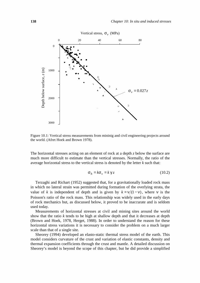
Measurements of vertical stress at various mining and civil engineering sites around the world confirm that this relationship is valid although, as illustrated in Figure 10.1, there is a significant amount of scatter in the measurements.

138 Chapter 10: In situ and induced stresses

Vertical stress, vσ (MPa)

0 20 40 60 80

Figure 10.1: Vertical stress measurements from mininig and civil engineering projects around the world. (Afret Hoek and Brown 1978). The horizontal stresses acting on an element of rock at a depth z below the surface are much more difficult to estimate than the vertical stresses. Normally, the ratio of the average horizontal stress to the vertical stress is denoted by the letter k such that:

zkk vh γ=σ=σ (10.2)

Terzaghi and Richart (1952) suggested that, for a gravitationally loaded rock mass

in which no lateral strain was permitted during formation of the overlying strata, the value of k is independent of depth and is given by )1( ν−ν=k , where ν is the Poisson's ratio of the rock mass. This relationship was widely used in the early days of rock mechanics but, as discussed below, it proved to be inaccurate and is seldom used today.

Measurements of horizontal stresses at civil and mining sites around the world show that the ratio k tends to be high at shallow depth and that it decreases at depth (Brown and Hoek, 1978, Herget, 1988). In order to understand the reason for these horizontal stress variations it is necessary to consider the problem on a much larger scale than that of a single site.

Sheorey (1994) developed an elasto-static thermal stress model of the earth. This model considers curvature of the crust and variation of elastic constants, density and thermal expansion coefficients through the crust and mantle. A detailed discussion on Sheorey’s model is beyond the scope of this chapter, but he did provide a simplified

0

1000

2000

3000

Dep

th b

elow

surf

ace,

z (m

)

zv 027.0=σ

In situ stresses 139

equation which can be used for estimating the horizontal to vertical stress ratio k. This equation is:

k Ezh= + +

0 25 7 0 001

1. . (10.3)

where z (m) is the depth below surface and Eh (GPa) is the average deformation modulus of the upper part of the earth’s crust measured in a horizontal direction. This direction of measurement is important particularly in layered sedimentary rocks, in which the deformation modulus may be significantly different in different directions.

A plot of this equation is given in Figure 10.2 for a range of deformation moduli. The curves relating k with depth below surface z are similar to those published by Brown and Hoek (1978), Herget (1988) and others for measured in situ stresses. Hence equation 7.3 is considered to provide a reasonable basis for estimating the value of k.

As pointed out by Sheorey, his work does not explain the occurrence of measured vertical stresses that are higher than the calculated overburden pressure, the presence of very high horizontal stresses at some locations or why the two horizontal stresses are seldom equal. These differences are probably due to local topographic and geological features that cannot be taken into account in a large scale model such as that proposed by Sheorey. k = horizontal stress / vertical stress 0 1 2 3 4

Figure 10.2: Ratio of horizontal to vertical stress for different deformation moduli based upon Sheorey’s equation. (After Sheorey 1994).

0

1000

2000

3000

hE (GPa) 10 25 50 75 100

Dep

th b

elow

surf

ace,

z (m

)


Where sensitivity studies have shown that the in situ stresses are likely to have a significant influence on the behaviour of underground openings, it is recommended that the in situ stresses should be measured. Suggestions for setting up a stress measuring programme are discussed later in this chapter.

10.3 The World stress map

The World Stress Map project, completed in July 1992, involved over 30 scientists from 18 countries and was carried out under the auspices of the International Lithosphere Project (Zoback, 1992). The aim of the project was to compile a global database of contemporary tectonic stress data. Currently over 7,300 stress orientation entries are included in a digital database. Of these approximately 4,400 observations are considered reliable tectonic stress indicators, recording horizontal stress orientations to within < ± 25°.

The data included in the World Stress Map are derived mainly from geological observations on earthquake focal mechanisms, volcanic alignments and fault slip interpretations. Less than 5% of the data is based upon hydraulic fracturing or overcoring measurements of the type commonly used in mining and civil engineering projects.

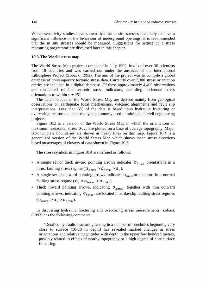
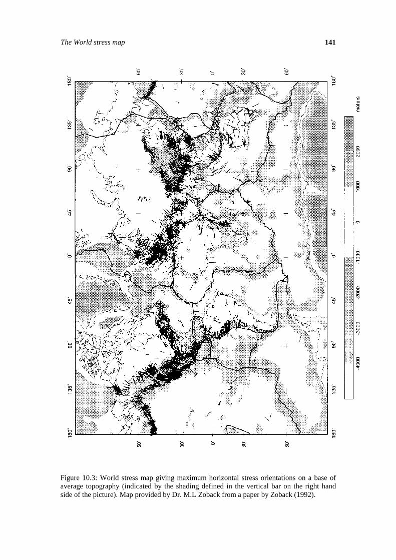
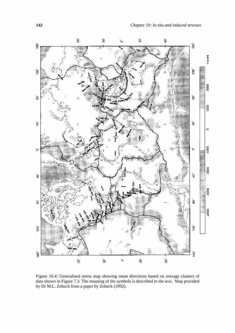
Figure 10.3 is a version of the World Stress Map in which the orientations of maximum horizontal stress σhmax are plotted on a base of average topography. Major tectonic plate boundaries are shown as heavy lines on this map. Figure 10.4 is a generalised version of the World Stress Map which shows mean stress directions based on averages of clusters of data shown in Figure 10.3.

The stress symbols in Figure 10.4 are defined as follows:

• A single set of thick inward pointing arrows indicates maxhσ orientations in a thrust faulting stress regime ( vhh σ>σ>σ minmax ).

• A single set of outward pointing arrows indicates minhσ orientations in a normal faulting stress regime ( minmax hhv σ>σ>σ ).

• Thick inward pointing arrows, indicating maxhσ , together with thin outward pointing arrows, indicating minhσ , are located in strike-slip faulting stress regimes ( minmax hvh σ>σ>σ ). In discussing hydraulic fracturing and overcoring stress measurements, Zoback

(1992) has the following comments:

‘Detailed hydraulic fracturing testing in a number of boreholes beginning very close to surface (10-20 m depth) has revealed marked changes in stress orientations and relative magnitudes with depth in the upper few hundred metres, possibly related to effects of nearby topography or a high degree of near surface fracturing.

The World stress map 141

Figure 10.3: World stress map giving maximum horizontal stress orientations on a base of average topography (indicated by the shading defined in the vertical bar on the right hand side of the picture). Map provided by Dr. M.L Zoback from a paper by Zoback (1992).


Figure 10.4: Generalised stress map showing mean directions based on average clusters of data shown in Figure 7.3. The meaning of the symbols is described in the text. Map provided by Dr M.L. Zoback from a paper by Zoback (1992).

Developing a stress measuring programme 143

Included in the category of ‘overcoring’ stress measurements are a variety of stress or strain relief measurement techniques. These techniques involve a three-dimensional measurement of the strain relief in a body of rock when isolated from the surrounding rock volume; the three-dimensional stress tensor can subsequently be calculated with a knowledge of the complete compliance tensor of the rock. There are two primary drawbacks with this technique which restricts its usefulness as a tectonic stress indicator: measurements must be made near a free surface, and strain relief is determined over very small areas (a few square millimetres to square centimetres). Furthermore, near surface measurements (by far the most common) have been shown to be subject to effects of local topography, rock anisotropy, and natural fracturing (Engelder and Sbar, 1984). In addition, many of these measurements have been made for specific engineering applications (e.g. dam site evaluation, mining work), places where topography, fracturing or nearby excavations could strongly perturb the regional stress field.’

Obviously, from a global or even a regional scale, the type of engineering stress

measurements carried out in a mine or on a civil engineering site are not regarded as very reliable. Conversely, the World Stress Map versions presented in Figures 10.3 and 10.4 can only be used to give first order estimates of the stress directions which are likely to be encountered on a specific site. Since both stress directions and stress magnitudes are critically important in the design of underground excavations, it follows that a stress measuring programme is essential in any major underground mining or civil engineering project.

10.4 Developing a stress measuring programme

Consider the example of a tunnel to be driven a depth of 1,000 m below surface in a hard rock environment. The depth of the tunnel is such that it is probable that in situ and induced stresses will be an important consideration in the design of the excavation. Typical steps that could be followed in the analysis of this problem are: a. During preliminary design, the information presented in equations 10.1, 10.2 and 10.3 can

be used to obtain a first rough estimate of the vertical and average horizontal stress in the vicinity of the tunnel. For a depth of 1,000 m, these equations give the vertical stress σv = 27 MPa , the ratio k = 1.3 (for Eh = 75 GPa) and hence the average horizontal stress σh= 35.1 MPa. A preliminary analysis of the stresses induced around the proposed tunnel (as described later in this chapter) shows that these induced stresses are likely to exceed the strength of the rock and that the question of stress measurement must be considered in more detail. Note that for many openings in strong rock at shallow depth, stress problems may not be significant and the analysis need not proceed any further.

b. For this particular case, stress problems are considered to be important. A typical next step would be to search the literature in an effort to determine whether the results of in situ stress measurement programmes are available for mines or civil engineering projects within a radius of say 50 km of the site. With luck, a few stress measurement results will be available for the region in which the tunnel is located and these results can be used to refine the analysis discussed above.

c. Assuming that the results of the analysis of induced stresses in the rock surrounding the proposed tunnel indicate that significant zones of rock failure are likely to develop, and that support costs are likely to be high, it is probably


justifiable to set up a stress measurement project on the site. These measurements can be carried out in deep boreholes from the surface, using hydraulic fracturing techniques, or from underground access using overcoring methods. The choice of the method and the number of measurements to be carried out depends upon the urgency of the problem, the availability of underground access and the costs involved in the project. Note that very few project organisations have access to the equipment required to carry out a stress measurement project and, rather than purchase this equipment, it may be worth bringing in an organisation which has the equipment and which specialises in such measurements.

Where regional tectonic features such as major faults are likely to be encountered the in situ stresses in the vicinity of the feature may be rotated with respect to the regional stress field. The stresses may be significantly different in magnitude from the values estimated from the general trends described earlier. These differences can be very important in the design of the openings and in the selection of support and, where it is suspected that this is likely to be the case, in situ stress measurements become an essential component of the overall design process.

10.5 Analysis of induced stresses

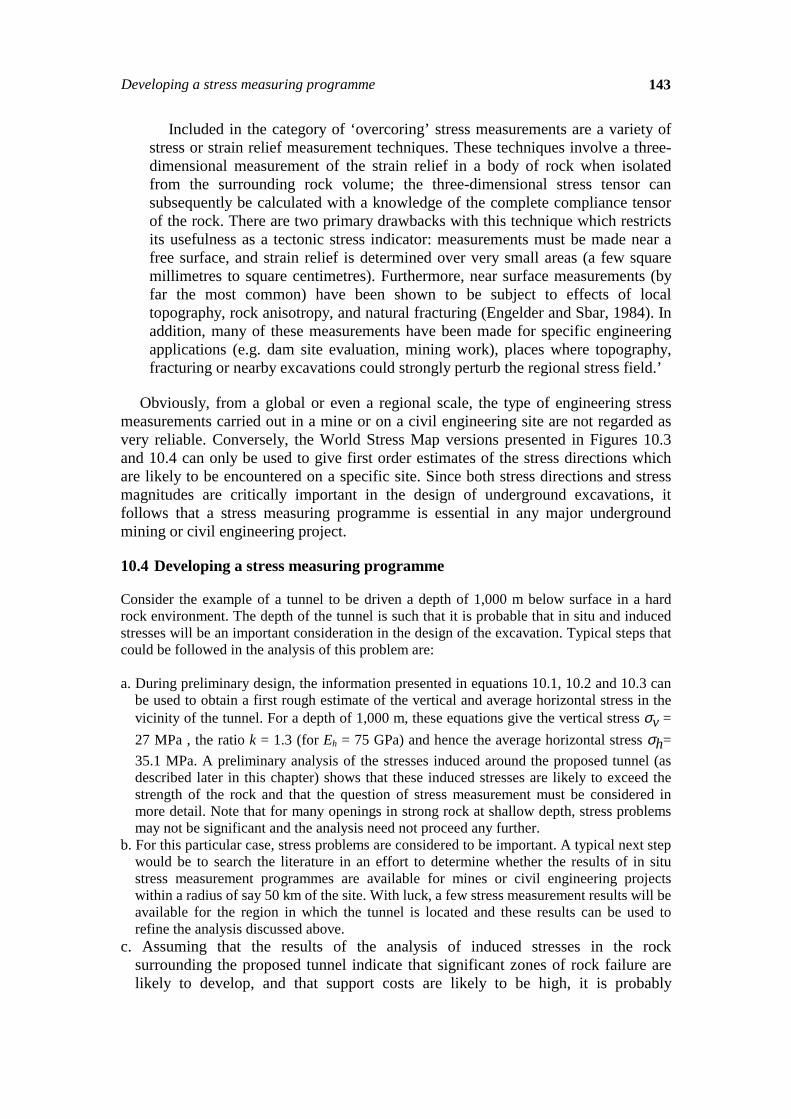
When an underground opening is excavated into a stressed rock mass, the stresses in the vicinity of the new opening are re-distributed. Consider the example of the stresses induced in the rock surrounding a horizontal circular tunnel as illustrated in Figure 10.5, showing a vertical slice normal to the tunnel axis.

Before the tunnel is excavated, the in situ stresses vσ , 1hσ and 2hσ are uniformly distributed in the slice of rock under consideration. After removal of the rock from within the tunnel, the stresses in the immediate vicinity of the tunnel are changed and new stresses are induced. Three principal stresses 21, σσ and 3σ acting on a typical element of rock are shown in Figure 10.5.

The convention used in rock mechanics is that compressive stresses are always positive and the three principal stresses are numbered such that 1σ is the largest and

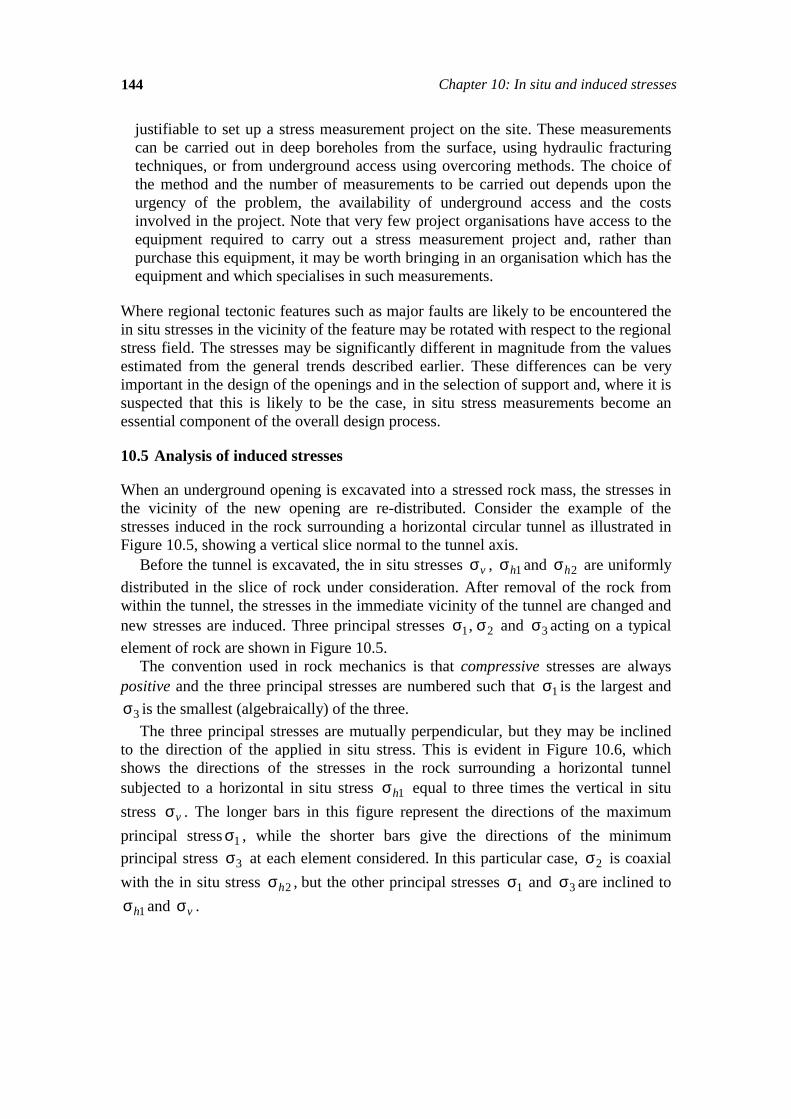
3σ is the smallest (algebraically) of the three. The three principal stresses are mutually perpendicular, but they may be inclined

to the direction of the applied in situ stress. This is evident in Figure 10.6, which shows the directions of the stresses in the rock surrounding a horizontal tunnel subjected to a horizontal in situ stress 1hσ equal to three times the vertical in situ stress vσ . The longer bars in this figure represent the directions of the maximum principal stress 1σ , while the shorter bars give the directions of the minimum principal stress 3σ at each element considered. In this particular case, 2σ is coaxial with the in situ stress 2hσ , but the other principal stresses 1σ and 3σ are inclined to

1hσ and vσ .

Analysis of induced stresses 145

Figure 10.5: Illustration of principal stresses induced in an element of rock close to a horizontal tunnel subjected to a vertical in situ stress vσ , a horizontal in situ stress 1hσ in a plane normal to the tunnel axis and a horizontal in situ stress 2hσ parallel to the tunnel axis.

Figure 10.6: Principal stress directions in the rock surrounding a horizontal tunnel subjected to a horizontal in situ stress 1hσ equal to 3 vσ , where vσ is the vertical in situ stress.

Vertical in situ stress vσ

Horizontal in situ stress 2hσ

Horizontal tunnel

Induced principal stresses

1σ

2σ

3σ Hor

izon

tal i

n si

tu st

ress

1hσ


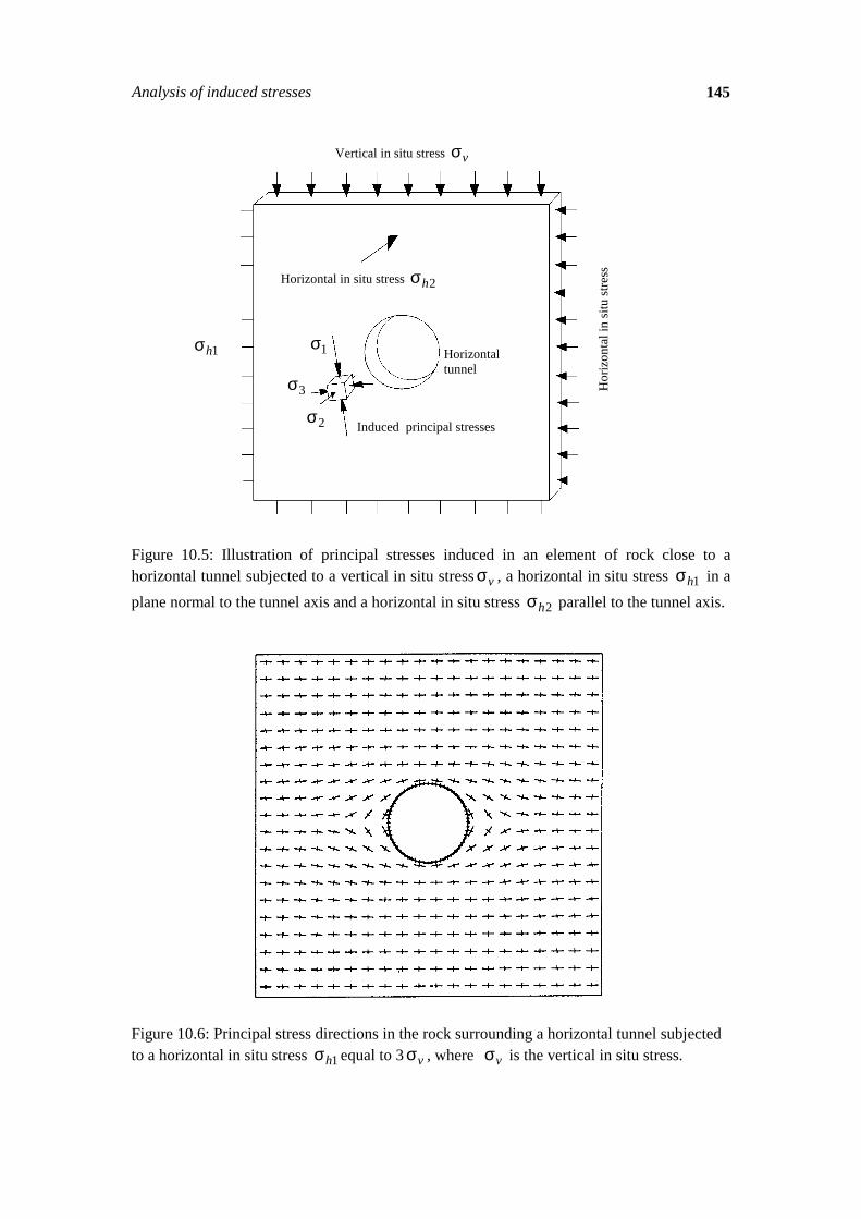
Figure 10.7: Contours of maximum and minimum principal stress magnitudes in the rock surrounding a horizontal tunnel, subjected to a vertical in situ stress of σv and a horizontal in situ stress of 3σv .

Contours of the magnitudes of the maximum principal stress 1σ and the minimum principal stress 3σ are given in Figure 10.7. This figure shows that the redistribution of stresses is concentrated in the rock close to the tunnel and that, at a distance of say three times the radius from the centre of the hole, the disturbance to the in situ stress field is negligible.

An analytical solution for the stress distribution in a stressed elastic plate containing a circular hole was published by Kirsch (1898) and this formed the basis for many early studies of rock behaviour around tunnels and shafts.

Following along the path pioneered by Kirsch, researchers such as Love (1927), Muskhelishvili (1953) and Savin (1961) published solutions for excavations of various shapes in elastic plates. A useful summary of these solutions and their application in rock mechanics was published by Brown in an introduction to a volume entitled Analytical and Computational Methods in Engineering Rock Mechanics (1987).

Closed form solutions still possess great value for conceptual understanding of behaviour and for the testing and calibration of numerical models. For design purposes, however, these models are restricted to very simple geometries and material models. They are of limited practical value. Fortunately, with the development of computers, many powerful programs which provide numerical solutions to these problems are now readily available. A brief review of some of these numerical solutions is given below.

Maximum principal stress vσσ1

Minimum principal stress vσσ3

8

4

3

2 1 0

1.2

1.0

0.8

1.0 1.2

0.6

Numerical methods of stress analysis 147

10.6 Numerical methods of stress analysis

Most underground excavations are irregular in shape and are frequently grouped close to other excavations. These groups of excavations can form a set of complex three-dimensional shapes. In addition, because of the presence of geological features such as faults and intrusions, the rock properties are seldom uniform within the rock volume of interest. Consequently, the closed form solutions described earlier are of limited value in calculating the stresses, displacements and failure of the rock mass surrounding underground excavations. Fortunately a number of computer-based numerical methods have been developed over the past few decades and these methods provide the means for obtaining approximate solutions to these problems.

Numerical methods for the analysis of stress driven problems in rock mechanics can be divided into two classes: • Boundary methods, in which only the boundary of the excavation is divided into

elements and the interior of the rock mass is represented mathematically as an infinite continuum.

• Domain methods, in which the interior of the rock mass is divided into

geometrically simple elements each with assumed properties. The collective behaviour and interaction of these simplified elements model the more complex overall behaviour of the rock mass. Finite element and finite difference methods are domain techniques which treat the rock mass as a continuum. The distinct element method is also a domain method which models each individual block of rock as a unique element.

These two classes of analysis can be combined in the form of hybrid models in

order to maximise the advantages and minimise the disadvantages of each method. It is possible to make some general observations about the two types of approaches

discussed above. In domain methods, a significant amount of effort is required to create the mesh that is used to divide the rock mass into elements. In the case of complex models, such as those containing multiple openings, meshing can become extremely difficult. The availability of highly optimised mesh-generators in many models makes this task much simpler than was the case when the mesh had to be created manually. In contrast, boundary methods require only that the excavation boundary be discretized and the surrounding rock mass is treated as an infinite continuum. Since fewer elements are required in the boundary method, the demand on computer memory and on the skill and experience of the user is reduced.

In the case of domain methods, the outer boundaries of the model must be placed sufficiently far away from the excavations in order that errors, arising from the interaction between these outer boundaries and the excavations, are reduced to an acceptable minimum. On the other hand, since boundary methods treat the rock mass as an infinite continuum, the far field conditions need only be specified as stresses acting on the entire rock mass and no outer boundaries are required. The main strength of boundary methods lies in the simplicity achieved by representing the rock mass as a continuum of infinite extent. It is this representation, however, that makes it difficult to incorporate variable material properties and the modelling of rock-support interaction. While techniques have been developed to allow some boundary element


modelling of variable rock properties, these types of problems are more conveniently modelled by domain methods.

Before selecting the appropriate modelling technique for particular types of problems, it is necessary to understand the basic components of each technique. 10.6.1 Boundary Element Method

The boundary element method derives its name from the fact that only the boundaries of the problem geometry are divided into elements. In other words, only the excavation surfaces, the free surface for shallow problems, joint surfaces where joints are considered explicitly and material interfaces for multi-material problems are divided into elements. In fact, several types of boundary element models are collectively referred to as ‘the boundary element method’. These models may be grouped as follows: 1. Indirect (Fictitious Stress) method, so named because the first step in the solution is

to find a set of fictitious stresses that satisfy prescribed boundary conditions. These stresses are then used in the calculation of actual stresses and displacements in the rock mass.

2. Direct method, so named because the displacements are solved directly for the

specified boundary conditions. 3. Displacement Discontinuity method, so named because it represents the result of an

elongated slit in an elastic continuum being pulled apart.

The differences between the first two methods are not apparent to the program user. The direct method has certain advantages in terms of program development, as will be discussed later in the section on Hybrid approaches.

The fact that a boundary element model extends ‘to infinity’ can also be a disadvantage. For example, a heterogeneous rock mass consists of regions of finite, not infinite, extent. Special techniques must be used to handle these situations. Joints are modelled explicitly in the boundary element method using the displacement discontinuity approach, but this can result in a considerable increase in computational effort. Numerical convergence is often found to be a problem for models incorporating many joints. For these reasons, problems, requiring explicit consideration of several joints and/or sophisticated modelling of joint constitutive behaviour, are often better handled by one of the domain methods such as finite elements.

A widely-used application of displacement discontinuity boundary elements is in the modelling of tabular ore bodies. Here, the entire ore seam is represented as a ‘discontinuity’ which is initially filled with ore. Mining is simulated by reduction of the ore stiffness to zero in those areas where mining has occurred, and the resulting stress redistribution to the surrounding pillars may be examined (Salamon, 1974, von Kimmelmann et al., 1984).

Further details on boundary element methods can be found in the book Boundary element methods in solid mechanics by Crouch and Starfield (1983).


10.6.2 Finite element and finite difference methods

In practice, the finite element method is usually indistinguishable from the finite difference method; thus, they will be treated here as one and the same. For the boundary element method, it was seen that conditions on a surface could be related to the state at all points throughout the remaining rock, even to infinity. In comparison, the finite element method relates the conditions at a few points within the rock (nodal points) to the state within a finite closed region formed by these points (the element). The physical problem is modelled numerically by dividing the entire problem region into elements.

The finite element method is well suited to solving problems involving heterogeneous or non-linear material properties, since each element explicitly models the response of its contained material. However, finite elements are not well suited to modelling infinite boundaries, such as occur in underground excavation problems. One technique for handling infinite boundaries is to discretize beyond the zone of influence of the excavation and to apply appropriate boundary conditions to the outer edges. Another approach has been to develop elements for which one edge extends to infinity i.e. so-called 'infinity' finite elements. In practice, efficient pre- and post-processors allow the user to perform parametric analyses and assess the influence of approximated far-field boundary conditions. The time required for this process is negligible compared to the total analysis time.

Joints can be represented explicitly using specific 'joint elements'. Different techniques have been proposed for handling such elements, but no single technique has found universal favour. Joint interfaces may be modelled, using quite general constitutive relations, though possibly at increased computational expense depending on the solution technique.

Once the model has been divided into elements, material properties have been assigned and loads have been prescribed, some technique must be used to redistribute any unbalanced loads and thus determine the solution to the new equilibrium state. Available solution techniques can be broadly divided into two classes - implicit and explicit. Implicit techniques assemble systems of linear equations that are then solved using standard matrix reduction techniques. Any material non-linearity is accounted for by modifying stiffness coefficients (secant approach) and/or by adjusting prescribed variables (initial stress or initial strain approach). These changes are made in an iterative manner such that all constitutive and equilibrium equations are satisfied for the given load state.

The response of a non-linear system generally depends upon the sequence of loading. Thus it is necessary that the load path modelled be representative of the actual load path experienced by the body. This is achieved by breaking the total applied load into load increments, each increment being sufficiently small, that solution convergence for the increment is achieved after only a few iterations. However, as the system being modelled becomes increasingly non-linear and the load increment represents an ever smaller portion of the total load, the incremental solution technique becomes similar to modelling the quasi-dynamic behaviour of the body, as it responds to gradual application of the total load.

In order to overcome this, a ‘dynamic relaxation’ solution technique was proposed (Otter et al., 1966) and first applied to geomechanics modelling by Cundall (1971). In this technique no matrices are formed. Rather, the solution proceeds explicitly -


unbalanced forces, acting at a material integration point, result in acceleration of the mass associated with the point; applying Newton's law of motion expressed as a difference equation yields incremental displacements; applying the appropriate constitutive relation produces the new set of forces, and so on marching in time, for each material integration point in the model. This solution technique has the advantage that both geometric and material non-linearities are accommodated, with relatively little additional computational effort as compared to a corresponding linear analysis, and computational expense increases only linearly with the number of elements used. A further practical advantage lies in the fact that numerical divergence usually results in the model predicting obviously anomalous physical behaviour. Thus, even relatively inexperienced users may recognise numerical divergence.

Most commercially available finite element packages use implicit (i.e. matrix) solution techniques. For linear problems and problems of moderate non-linearity, implicit techniques tend to perform faster than explicit solution techniques. However, as the degree of non-linearity of the system increases, imposed loads must be applied in smaller increments which implies a greater number of matrix re-formations and reductions, and hence increased computational expense. Therefore, highly non-linear problems are best handled by packages using an explicit solution technique.

10.6.3 Distinct Element Method

In ground conditions conventionally described as blocky (i.e. where the spacing of the joints is of the same order of magnitude as the excavation dimensions), intersecting joints form wedges of rock that may be regarded as rigid bodies. That is, these individual pieces of rock may be free to rotate and translate, and the deformation, that takes place at block contacts, may be significantly greater than the deformation of the intact rock, so that individual wedges may be considered rigid. For such conditions it is usually necessary to model many joints explicitly. However, the behaviour of such systems is so highly non-linear, that even a jointed finite element code, employing an explicit solution technique, may perform relatively inefficiently.

An alternative modelling approach is to develop data structures that represent the blocky nature of the system being analysed. Each block is considered a unique free body that may interact at contact locations with surrounding blocks. Contacts may be represented by the overlaps of adjacent blocks, thereby avoiding the necessity of unique joint elements. This has the added advantage that arbitrarily large relative displacements at the contact may occur, a situation not generally tractable in finite element codes.

Due to the high degree of non-linearity of the systems being modelled, explicit solution techniques are favoured for distinct element codes. As is the case for finite element codes employing explicit solution techniques, this permits very general constitutive modelling of joint behaviour with little increase in computational effort and results in computation time being only linearly dependent on the number of elements used. The use of explicit solution techniques places fewer demands on the skills and experience than the use of codes employing implicit solution techniques.

Although the distinct element method has been used most extensively in academic environments to date, it is finding its way into the offices of consultants, planners and designers. Further experience in the application of this powerful modelling tool to practical design situations and subsequent documentation of these case histories is


required, so that an understanding may be developed of where, when and how the distinct element method is best applied.

10.6.4 Hybrid approaches

The objective of a hybrid method is to combine the above methods in order to eliminate undesirable characteristics while retaining as many advantages as possible. For example, in modelling an underground excavation, most non-linearity will occur close to the excavation boundary, while the rock mass at some distance will behave in an elastic fashion. Thus, the near-field rock mass might be modelled, using a distinct element or finite element method, which is then linked at its outer limits to a boundary element model, so that the far-field boundary conditions are modelled exactly. In such an approach, the direct boundary element technique is favoured as it results in increased programming and solution efficiency.

Lorig and Brady (1984) used a hybrid model consisting of a discrete element model for the near field and a boundary element model for the far field in a rock mass surrounding a circular tunnel.

10.6.5 Two-dimensional and three-dimensional models

A two-dimensional model, such as that illustrated in Figure 10.5, can be used for the analysis of stresses and displacements in the rock surrounding a tunnel, shaft or borehole, where the length of the opening is much larger than its cross-sectional dimensions. The stresses and displacements in a plane, normal to the axis of the opening, are not influenced by the ends of the opening, provided that these ends are far enough away.

On the other hand, a an underground powerhouse of crusher chamber has a much more equi-dimensional shape and the effect of the end walls cannot be neglected. In this case, it is much more appropriate to carry out a three-dimensional analysis of the stresses and displacements in the surrounding rock mass. Unfortunately, this switch from two to three dimensions is not as simple as it sounds and there are relatively few good three-dimensional numerical models, which are suitable for routine stress analysis work in a typical mining environment.

EXAMINE3D1 is a three-dimensional boundary element programs that provide a

starting point for an analysis of a problem in which the three-dimensional geometry of the openings is important. Such three-dimensional analyses provide clear indications of stress concentrations and of the influence of three-dimensional geometry. In many cases, it is possible to simplify the problem to two-dimensions by considering the stresses on critical sections identified in the three-dimensional model.

More sophisticated three-dimensional finite element models such as VISAGE2 are available, but are not particularly easy to use at the present time. In addition, definition of the input parameters and interpretation of the results of these models would stretch the capabilities of all but the most experienced modellers. It is probably best to leave this type of modelling in the hands of these specialists.

1Available from Available from Rocscience Inc., 31 Balsam Avenue, Toronto, Ontario, Canada M4E 3B5, Fax 1 416 698 0908, Phone 1 416 698 8217, Email: [email protected], Internet http://www.rocscience.com. 2Available from Vector International Processing Systems Ltd., Suites B05 and B06, Surrey House, 34 Eden Street, Kingston on Thames, KT1 1ER, England. Fax 44 81 541 4550, Phone 44 81 549 3444.


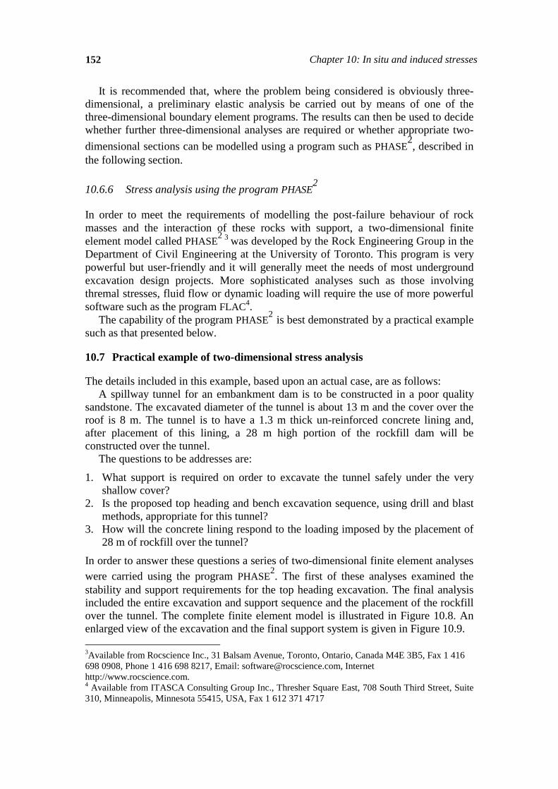
It is recommended that, where the problem being considered is obviously three-dimensional, a preliminary elastic analysis be carried out by means of one of the three-dimensional boundary element programs. The results can then be used to decide whether further three-dimensional analyses are required or whether appropriate two-dimensional sections can be modelled using a program such as PHASE

2, described in the following section.

10.6.6 Stress analysis using the program PHASE

2

In order to meet the requirements of modelling the post-failure behaviour of rock masses and the interaction of these rocks with support, a two-dimensional finite element model called PHASE2 3 was developed by the Rock Engineering Group in the Department of Civil Engineering at the University of Toronto. This program is very powerful but user-friendly and it will generally meet the needs of most underground excavation design projects. More sophisticated analyses such as those involving thremal stresses, fluid flow or dynamic loading will require the use of more powerful software such as the program FLAC4. The capability of the program PHASE2 is best demonstrated by a practical example such as that presented below.

10.7 Practical example of two-dimensional stress analysis

The details included in this example, based upon an actual case, are as follows: A spillway tunnel for an embankment dam is to be constructed in a poor quality

sandstone. The excavated diameter of the tunnel is about 13 m and the cover over the roof is 8 m. The tunnel is to have a 1.3 m thick un-reinforced concrete lining and, after placement of this lining, a 28 m high portion of the rockfill dam will be constructed over the tunnel. The questions to be addresses are: 1. What support is required on order to excavate the tunnel safely under the very

shallow cover? 2. Is the proposed top heading and bench excavation sequence, using drill and blast

methods, appropriate for this tunnel? 3. How will the concrete lining respond to the loading imposed by the placement of

28 m of rockfill over the tunnel? In order to answer these questions a series of two-dimensional finite element analyses were carried using the program PHASE2. The first of these analyses examined the stability and support requirements for the top heading excavation. The final analysis included the entire excavation and support sequence and the placement of the rockfill over the tunnel. The complete finite element model is illustrated in Figure 10.8. An enlarged view of the excavation and the final support system is given in Figure 10.9. 3Available from Rocscience Inc., 31 Balsam Avenue, Toronto, Ontario, Canada M4E 3B5, Fax 1 416 698 0908, Phone 1 416 698 8217, Email: [email protected], Internet http://www.rocscience.com. 4 Available from ITASCA Consulting Group Inc., Thresher Square East, 708 South Third Street, Suite 310, Minneapolis, Minnesota 55415, USA, Fax 1 612 371 4717

Practical example of two-dimensional stress analysis 153

Figure 10.8: Finite element model showing mesh geometry and boundary conditions. The final support system used for this case is also shown and will be discussed in the text which follows.

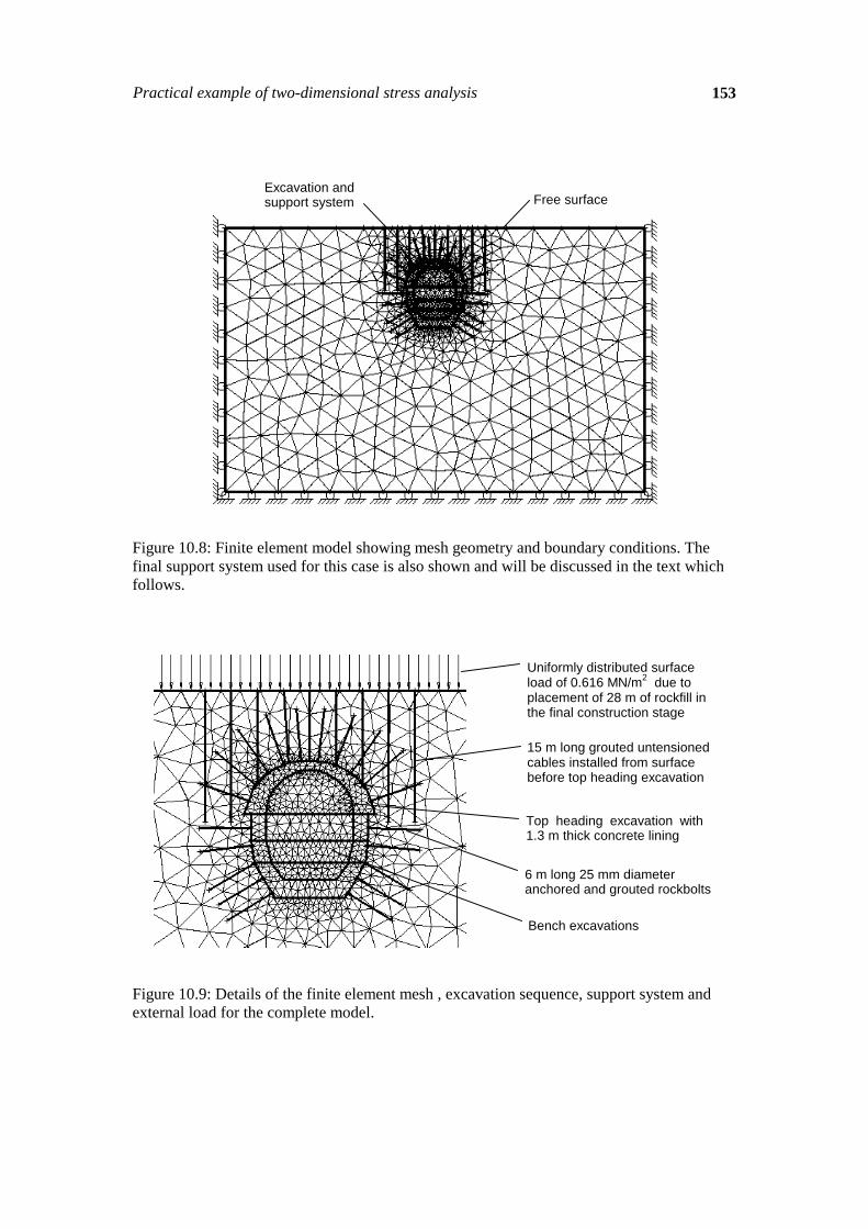
Figure 10.9: Details of the finite element mesh , excavation sequence, support system and external load for the complete model.

Free surface Excavation and support system

Uniformly distributed surface load of 0.616 MN/m2 due to placement of 28 m of rockfill in the final construction stage

15 m long grouted untensioned cables installed from surface before top heading excavation

Top heading excavation with 1.3 m thick concrete lining

6 m long 25 mm diameter anchored and grouted rockbolts

Bench excavations


The rock mass is a poor quality sandstone that, being close to surface, is heavily jointed. The mechanical properties5 assumed for this rock mass are a cohesive strength c = 0.04 MPa, a friction angle φ = 40° and a modulus of deformation E = 1334 MPa. No in situ stress measurements are available but, because of the location of the tunnel in the valley side, it has been assumed that the horizontal stress normal to the tunnel axis has been reduced by stress relief. The model is loaded by gravity and a ratio of horizontal to vertical stress or 0.5 is assumed. 10.7.1 Analysis of top heading stability

A simplified version of the model illustrated in Figures 10.8 and 10.9 was used to analyse the stability and support requirements for the top heading. This model did excluded the concrete lining and the bench excavations.

The first model was used to examine the conditions for a full-face excavation of the top heading without any support. This is always a useful starting point in any tunnel support design study since it gives the designer a clear picture of the magnitude of the problems that have to be dealt with.

The model was loaded in two stages. The first stage involved the model without any excavations and this was created by assigning the material within the excavation boundary the properties of the surrounding rock mass. This first stage is carried out in order to allow the model to consolidate under gravitational loading It is required in order to create a reference against which subsequent displacements in the model can be measured.

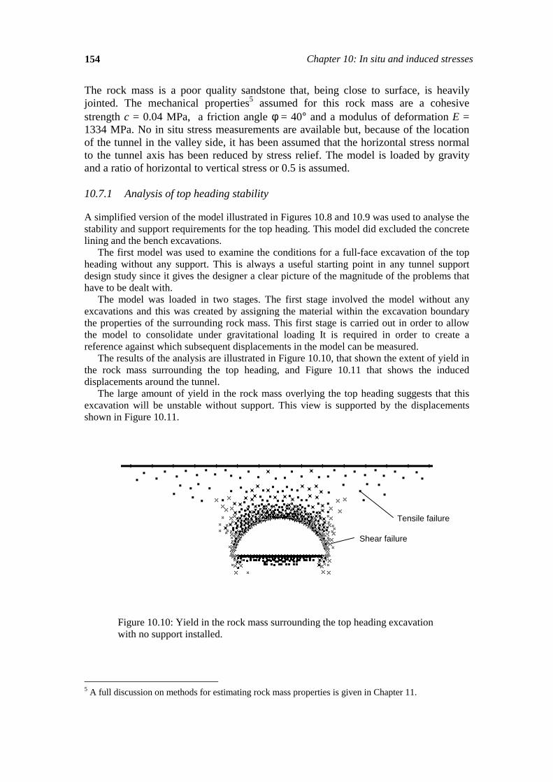
The results of the analysis are illustrated in Figure 10.10, that shown the extent of yield in the rock mass surrounding the top heading, and Figure 10.11 that shows the induced displacements around the tunnel.

The large amount of yield in the rock mass overlying the top heading suggests that this excavation will be unstable without support. This view is supported by the displacements shown in Figure 10.11.

Figure 10.10: Yield in the rock mass surrounding the top heading excavation with no support installed.

5 A full discussion on methods for estimating rock mass properties is given in Chapter 11.

Shear failure

Tensile failure


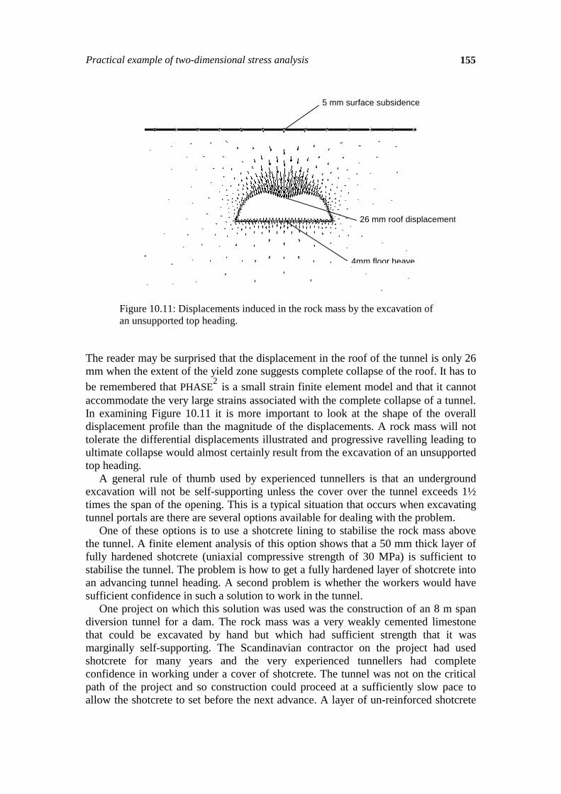
Figure 10.11: Displacements induced in the rock mass by the excavation of an unsupported top heading.

The reader may be surprised that the displacement in the roof of the tunnel is only 26 mm when the extent of the yield zone suggests complete collapse of the roof. It has to be remembered that PHASE2 is a small strain finite element model and that it cannot accommodate the very large strains associated with the complete collapse of a tunnel. In examining Figure 10.11 it is more important to look at the shape of the overall displacement profile than the magnitude of the displacements. A rock mass will not tolerate the differential displacements illustrated and progressive ravelling leading to ultimate collapse would almost certainly result from the excavation of an unsupported top heading. A general rule of thumb used by experienced tunnellers is that an underground excavation will not be self-supporting unless the cover over the tunnel exceeds 1½ times the span of the opening. This is a typical situation that occurs when excavating tunnel portals are there are several options available for dealing with the problem. One of these options is to use a shotcrete lining to stabilise the rock mass above the tunnel. A finite element analysis of this option shows that a 50 mm thick layer of fully hardened shotcrete (uniaxial compressive strength of 30 MPa) is sufficient to stabilise the tunnel. The problem is how to get a fully hardened layer of shotcrete into an advancing tunnel heading. A second problem is whether the workers would have sufficient confidence in such a solution to work in the tunnel. One project on which this solution was used was the construction of an 8 m span diversion tunnel for a dam. The rock mass was a very weakly cemented limestone that could be excavated by hand but which had sufficient strength that it was marginally self-supporting. The Scandinavian contractor on the project had used shotcrete for many years and the very experienced tunnellers had complete confidence in working under a cover of shotcrete. The tunnel was not on the critical path of the project and so construction could proceed at a sufficiently slow pace to allow the shotcrete to set before the next advance. A layer of un-reinforced shotcrete

5 mm surface subsidence

26 mm roof displacement

4mm floor heave


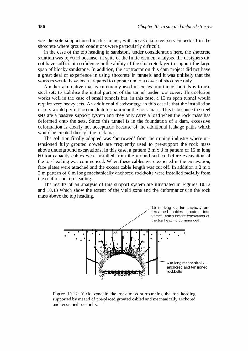
was the sole support used in this tunnel, with occasional steel sets embedded in the shotcrete where ground conditions were particularly difficult. In the case of the top heading in sandstone under consideration here, the shotcrete solution was rejected because, in spite of the finite element analysis, the designers did not have sufficient confidence in the ability of the shotcrete layer to support the large span of blocky sandstone. In addition, the contractor on this dam project did not have a great deal of experience in using shotcrete in tunnels and it was unlikely that the workers would have been prepared to operate under a cover of shotcrete only. Another alternative that is commonly used in excavating tunnel portals is to use steel sets to stabilise the initial portion of the tunnel under low cover. This solution works well in the case of small tunnels but, in this case, a 13 m span tunnel would require very heavy sets. An additional disadvantage in this case is that the installation of sets would permit too much deformation in the rock mass. This is because the steel sets are a passive support system and they only carry a load when the rock mass has deformed onto the sets. Since this tunnel is in the foundation of a dam, excessive deformation is clearly not acceptable because of the additional leakage paths which would be created through the rock mass. The solution finally adopted was ‘borrowed’ from the mining industry where un-tensioned fully grouted dowels are frequently used to pre-support the rock mass above underground excavations. In this case, a pattern 3 m x 3 m pattern of 15 m long 60 ton capacity cables were installed from the ground surface before excavation of the top heading was commenced. When these cables were exposed in the excavation, face plates were attached and the excess cable length was cut off. In addition a 2 m x 2 m pattern of 6 m long mechanically anchored rockbolts were installed radially from the roof of the top heading. The results of an analysis of this support system are illustrated in Figures 10.12 and 10.13 which show the extent of the yield zone and the deformations in the rock mass above the top heading.

Figure 10.12: Yield zone in the rock mass surrounding the top heading supported by meand of pre-placed grouted cabled and mechanically anchored and tensioned rockbolts.

15 m long 60 ton capacity un-tensioned cables grouted intovertical holes before excavation ofthe top heading commenced

6 m long mechanically anchored and tensioned rockbolts


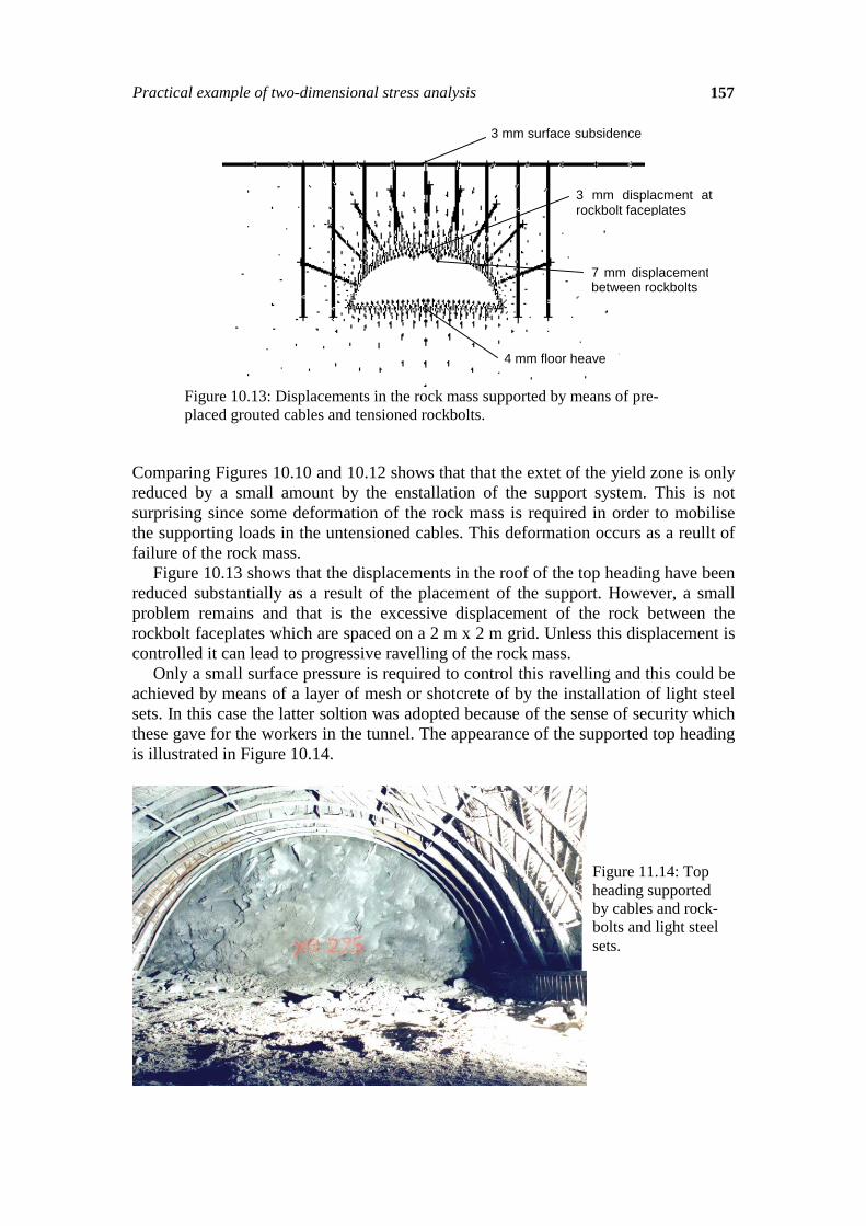
Figure 10.13: Displacements in the rock mass supported by means of pre-placed grouted cables and tensioned rockbolts.

Comparing Figures 10.10 and 10.12 shows that that the extet of the yield zone is only reduced by a small amount by the enstallation of the support system. This is not surprising since some deformation of the rock mass is required in order to mobilise the supporting loads in the untensioned cables. This deformation occurs as a reullt of failure of the rock mass. Figure 10.13 shows that the displacements in the roof of the top heading have been reduced substantially as a result of the placement of the support. However, a small problem remains and that is the excessive displacement of the rock between the rockbolt faceplates which are spaced on a 2 m x 2 m grid. Unless this displacement is controlled it can lead to progressive ravelling of the rock mass. Only a small surface pressure is required to control this ravelling and this could be achieved by means of a layer of mesh or shotcrete of by the installation of light steel sets. In this case the latter soltion was adopted because of the sense of security which these gave for the workers in the tunnel. The appearance of the supported top heading is illustrated in Figure 10.14.


3 mm displacment at rockbolt faceplates

7 mm displacementbetween rockbolts

4 mm floor heave

Figure 11.14: Top heading supported by cables and rock-bolts and light steel sets.


10.7.2 Analysis of complete excavation

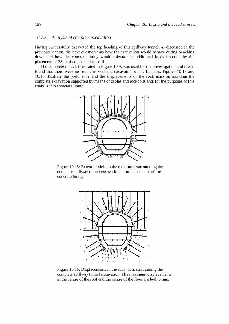
Having successfully excavated the top heading of this spillway tunnel, as discussed in the previous section, the next question was how the excavation would behave during benching down and how the concrete lining would tolerate the additional loads imposed by the placement of 28 m of compacted rock fill. The complete model, illustrated in Figure 10.9, was used for this investigation and it was found that there were no problems with the excavation of the benches. Figures 10.15 and 10.16 illustrate the yield zone and the displacements of the rock mass surrounding the complete excavation supported by means of cables and rockbolts and, for the purposes of this study, a thin shotcrete lining.

Figure 10.15: Extent of yield in the rock mass surrounding the complete spillway tunnel excavation before placement of the concrete lining.

Figure 10.16: Displacements in the rock mass surrounding the complete spillway tunnel excavation. The maximum displacements in the centre of the roof and the centre of the floor are both 5 mm.


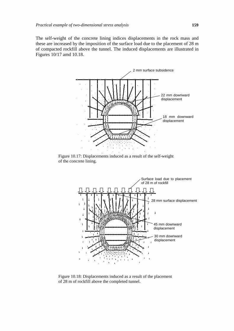
The self-weight of the concrete lining indices displacements in the rock mass and these are increased by the imposition of the surface load due to the placement of 28 m of compacted rockfill above the tunnel. The induced displacements are illustrated in Figures 10/17 amd 10.18.

Figure 10.17: Displacements induced as a result of the self-weight of the concrete lining.

Figure 10.18: Displacements induced as a result of the placement of 28 m of rockfill above the completed tunnel.


22 mm downward displacement


Surface load due to placementof 28 m of rockfill

28 mm surface displacement




Figures 10.17 and 10.18 show that significant displacements are induced as a result of the casting of the concrete lining and the subsequent placement of the rockfill above the tunnel. No failure of the concrete lining was shown by this analysis, in spite of the assumption of a very weak concrete (10 MPa uniaxial compressive strength). The only problem that could be anticipated from the placement of the rockfill was the possibility of bending of the entire length of the concrete lining and the formation of tensile cracks normal to the tunnel axis. It was therefore recommended that the concrete lining be carefully inspected for such cracks after the completion of the rockfill. Repair of such cracks by dental concrete and grouting would not be a major problem but, in any case, it proved not to be necessary. 10.7.3 Conclusion

The analysis presented on the preceding pages is intended to demonstrate how a numerical analysis should be used as a tool to aid designers. In all cases, practical issues take precedence and the results of the analysis should only be used to guide the practical decisions and to clarify matters of doubt or uncertainty. Given the assumptions that have to be made in the construction of an analysis of this type, it would be very unwise for the designer to place too much credence in the results of the analysis and to allow all his or her decisions to be driven by these results. A discussion of the results with an experienced tunnel contractor will soon dispel any misconceptions that the tunnel designer will have acquired as the results of such a theoretical analysis and such a discussion is an essential part of any practical design process.

10 In situ and induced stresses - Strona główna AGHhome.agh.edu.pl/~cala/hoek/Chapter10.pdf · in...

Documents

Transcript of 10 In situ and induced stresses - Strona główna AGHhome.agh.edu.pl/~cala/hoek/Chapter10.pdf · in...