IN SITU MEASUREMENT OF FATIGUE INDUCED CRACK GROWTH …

Graduate Theses, Dissertations, and Problem Reports

2019

IN SITU MEASUREMENT OF FATIGUE INDUCED CRACK GROWTH IN SITU MEASUREMENT OF FATIGUE INDUCED CRACK GROWTH

IN INCONEL 718 USING DIRECT CURRENT POTENTIAL DROP IN INCONEL 718 USING DIRECT CURRENT POTENTIAL DROP

METHOD METHOD

Joel C. Lindsay West Virginia University, [email protected]

Follow this and additional works at: https://researchrepository.wvu.edu/etd

Part of the Materials Science and Engineering Commons, and the Mechanical Engineering Commons

Recommended Citation Recommended Citation Lindsay, Joel C., "IN SITU MEASUREMENT OF FATIGUE INDUCED CRACK GROWTH IN INCONEL 718 USING DIRECT CURRENT POTENTIAL DROP METHOD" (2019). Graduate Theses, Dissertations, and Problem Reports. 4050. https://researchrepository.wvu.edu/etd/4050

This Thesis is protected by copyright and/or related rights. It has been brought to you by the The Research Repository @ WVU with permission from the rights-holder(s). You are free to use this Thesis in any way that is permitted by the copyright and related rights legislation that applies to your use. For other uses you must obtain permission from the rights-holder(s) directly, unless additional rights are indicated by a Creative Commons license in the record and/ or on the work itself. This Thesis has been accepted for inclusion in WVU Graduate Theses, Dissertations, and Problem Reports collection by an authorized administrator of The Research Repository @ WVU. For more information, please contact [email protected].

https://researchrepository.wvu.edu/

https://researchrepository.wvu.edu/

https://researchrepository.wvu.edu/etd

https://researchrepository.wvu.edu/etd?utm_source=researchrepository.wvu.edu%2Fetd%2F4050&utm_medium=PDF&utm_campaign=PDFCoverPages

http://network.bepress.com/hgg/discipline/285?utm_source=researchrepository.wvu.edu%2Fetd%2F4050&utm_medium=PDF&utm_campaign=PDFCoverPages

http://network.bepress.com/hgg/discipline/293?utm_source=researchrepository.wvu.edu%2Fetd%2F4050&utm_medium=PDF&utm_campaign=PDFCoverPages

https://researchrepository.wvu.edu/etd/4050?utm_source=researchrepository.wvu.edu%2Fetd%2F4050&utm_medium=PDF&utm_campaign=PDFCoverPages

mailto:[email protected]

IN SITU MEASUREMENT OF FATIGUE INDUCED CRACK GROWTH IN INCONEL

718 USING DIRECT CURRENT POTENTIAL DROP METHOD

Joel C. Lindsay

Thesis submitted

to the Benjamin M. Statler College of

Engineering and Mineral Resources

at West Virginia University

in partial fulfillment of the requirements

for the degree of

Master of Science in

Mechanical Engineering

Terence Musho, Ph.D., Chair

Stefanos Papanikolaou, Ph.D.

Bruce Kang, Ph.D.

Department of Mechanical and Aerospace Engineering

Morgantown, West Virginia

2019

Keywords: Fatigue, Crack Growth, Inconel 718, DCPD

Copyright 2019 Joel C. Lindsay

Abstract

IN SITU MEASUREMENT OF FATIGUE INDUCED CRACK GROWTH IN INCONEL

718 USING DIRECT CURRENT POTENTIAL DROP METHOD

Joel C. Lindsay

With recent advances in air breathable engines comes more extreme temperature

environments that engine components must tolerate. During the design of these engines, it is

necessary to understand how material fatigue failures occur at these new, higher operating

temperatures. In providing understanding, the following fundamental study focuses on the

statistical nature of crack jumps (changes in crack length over time) during fatigue in a

polycrystalline nickel-based superalloy, Inconel 718 (IN718). In situ measurement of the crack

length at several loading conditions were conducted using a direct current potential drop

(DCPD) measurement method. Experimental data was collected at six different fatigue peak

loads (R=0.15) for a statistically significant number of trials (n≥17). Calibration curves to relate

electrical potential to crack length were derived from FEA and compared to analytical

equations. It was determined that the mean normalized change in crack length over subsequent

cycles increases with peak load. The standard deviation of the crack lengths remains constant

for all loading cases. The signal-to-noise ratio was found to be best at or above a peak load of

1600N (29.65% of YS) for the given sample geometry. Results of the normalized change in

crack length for a single case deviated from a Gaussian distribution. However, when all trials

were considered at a single load, the distribution of the normalized change in crack length

conformed to a Gaussian distribution. This lack of conformity for a single case can be

explained by the history dependence of prior crack events on the crack growth for an individual

specimen. This temporal information as the crack evolves, which is often overlooked in fatigue

experiments, is hypothesized to be well suited for a machine learning approach that can better

predict fatigue failures in superalloys.

iii

Table of Contents

Abstract ..................................................................................................................................... ii

List of Tables ........................................................................................................................... iv

List of Figures .......................................................................................................................... iv

List of Symbols and Abbreviations.......................................................................................... vi

1. Introduction .................................................................................................................... 1

2. Background .................................................................................................................... 3

2.1 Materials ................................................................................................................. 3

2.2 Composition............................................................................................................ 5

2.3 Material Properties ................................................................................................. 8

2.4 Fatigue .................................................................................................................... 8

2.5 Microstructure Effects on Fatigue .......................................................................... 9

2.6 Crack Measurement .............................................................................................. 10

3. Experimental Method................................................................................................... 13

3.1 Test Specimen Design .......................................................................................... 14

3.2 Machine Setup ...................................................................................................... 16

3.3 Analytical and FEA Comparison .......................................................................... 16

3.4 Material Properties ............................................................................................... 18

3.5 Test Parameters ..................................................................................................... 19

3.6 Data Processing .................................................................................................... 21

4. Results and Discussion: ............................................................................................... 24

4.1 Test Characteristics ............................................................................................... 24

4.2 Crack Characteristics ............................................................................................ 25

4.3 Crack Initiation ..................................................................................................... 26

4.4 SEM Imaging and Analysis .................................................................................. 27

4.5 Noise Qualification and Quantification ................................................................ 29

5. Conclusion ................................................................................................................... 34

5.1 Future Work .......................................................................................................... 34

Bibliography ........................................................................................................................... 35

Appendix A: Supplementary Plots.......................................................................................... 37

Appendix B: Python Script For Data Processing .................................................................... 42

Appendix C: Matlab Script For Data Processing .................................................................... 45

Appendix D: Matlab Plotting Script ....................................................................................... 51

iv

List of Tables

Table 1 – IN718 Chemical Composition [5]............................................................................. 5

Table 2 - Summary of the theoretical and actual min and max loads ..................................... 21

Table 3 - Testing and data processing characteristics ............................................................. 22

List of Figures

Figure 1 - Distribution of superalloy components in a gas turbine engine ............................... 4

Figure 2(A) - Crystal structures of the solid solution phase, γ (FCC) ...................................... 7

Figure 2(B) - Crystal structure of γ′ (FCC) phase..................................................................... 7

Figure 2(C) - Crystal structure of γ′′ (D022) phase .................................................................... 7

Figure 2(D) - Crystal Structure of δ (D0a) phase ...................................................................... 7

Figure 3(A) - SEM image of δ, γ′, and γ″ phases. .................................................................. 10

Figure 4(B) - TEM micrograph of δ and γ″ phases [16, 17]. .................................................. 10

Figure 5 - Lines of constant electric potential ........................................................................ 12

Figure 6(A) - Shows the Sunkko 709A spot welding machine .............................................. 14

Figure 5(B) - An image of the test specimen .......................................................................... 14

Figure 5(C) - Image of the fatigue testing setup ..................................................................... 14

Figure 6(A) - Schematic of Fatigue Specimen ....................................................................... 15

Figure 6(B) - Setup of Fatigue Test ........................................................................................ 15

Figure 7 - H. Johnson Analytical Calibration Curve Compared to FEA Derived Curve ....... 17

Figure 8 - Experimental Stress Strain Curve for Plate Inconel 718 ........................................ 19

Figure 9 - Loading cycles for three cases (1600N, 1700N, 1800N) ....................................... 20

v

Figure 10(A) – Crack length for single runs of each loading procedure. ............................... 24

Figure 10(B) - Average crack length vs. loading cycle number ............................................. 24

Figure 11 - Plot of Δa/ΔN versus the stress intensity factor ................................................... 25

Figure 12 – Averaged normalized crack growth curves up to a crack length of 0.1mm ........ 26

Figure 13 – Distributions showing the number of cycles needed to reach a crack length of

0.1mm for individual trials ..................................................................................................... 27

Figure 14(A) - Crack initiation point ...................................................................................... 28

Figure 14(B) - Zoomed in image along the crack path ........................................................... 28

Figure 14(C) - Termination zone of crack .............................................................................. 28

Figure 15 - Noise plot of a specimen under zero load ............................................................ 30

Figure 16(A) - Fmax=1800N plot of crack jump distribution .................................................. 32

Figure 16(B) - Fmax=1800N plot of crack jump distribution averaged across all 1800N runs 32

Figure 17 - Relative probability distribution of crack jumps .................................................. 33

Figure 1A (A) - Fmax=1800N plot of crack jump distribution ................................................ 37

Figure 1A (B) - Fmax=1800N plot of crack jump distribution averaged across all 1800N runs

................................................................................................................................................. 37



................................................................................................................................................. 38



................................................................................................................................................. 39

Figure 4A - Normalized Δa/ΔN Noise Plot vs hold Cycle for 1400N .................................... 40

vi



List of Symbols and Abbreviations

Symbols Definition

𝑑𝑎 Change in crack length

𝑑𝑁 Change in cycle

𝐶 Material constants

Δ𝐾 Stress intensity range

𝑚 Material constant

𝑎 Crack length from edge

𝑎0 Initial crack length (10mm)

𝑉(𝑎) Measured voltage as a function of crack length

𝑐(𝑎) Coordinate proportionality as a function of crack length

𝑢1(𝑎) Elliptical coordinate position of voltage measurement

𝑢0(𝑎) Elliptical coordinate position of slot boundary

𝑥𝑒 Crack x position in elliptical coordinates

𝑦𝑒 Crack y position in elliptical coordinates

𝑢 Radial distance from centerline in elliptical coordinates

𝑣 Angle from starting axis in elliptical coordinates

𝑊 Width of Test Specimen

𝜋 Mathematical constant

vii

𝑦 Distance from the crack to the measurement probes in the y-direction

𝑉0 Initial voltage at a crack length of 𝑎0

𝐾𝐼 Stress intensity at a load of I

𝜎 Uniform stress across the specimen

Abbreviations

IN718 Inconel 718

DCPD Direct Current Potential Drop

ASTM American Society for Testing and Materials

SEM Scanning Electron Microscopy

MTS Material Testing Systems

EDM Electric Discharge Machined

FEA Finite Element Analysis

PSB Persistent Slip Bands

1

1. Introduction

With the recent move to reduce carbon emissions across many counties and the constant

goal of reducing operation cost, gas turbine efficiency can achieve both goals and has been

increasing steadily over the past 50 years [1]. One of the methods that have been employed to

increase gas turbine efficiency is to have turbines operate at higher temperatures [2]. However,

higher temperatures require new materials and alloys, as well as a better understanding of the

basic physics that may drive materials informatics [3].

Regarding mechanical response, a better understanding of this physics in various

materials has coincided with the development of new predictive models for failure

mechanisms. A common superalloy used in the disk of turbines is Inconel 718 (IN718), a

nickel-based alloy that is designed to withstand extreme temperatures under high creep load

conditions. The main constitutive elements in this type of superalloys are nickel, cobalt, and

iron with a precisely prescribed precipitate-hardened microstructure that provides high

strength, high operating temperatures, as well as creep and oxidation resistance. The attributes

of IN718 come from the combination of its constitutive elements and microstructure but the

microstructure is the driving feature that impedes and govern the crack initiation and growth

in this material.

However, structural health monitoring has been typically limited in qualitative

assessments of isolated microstructural observations. Beyond the study of averages, a

fundamental understanding of crack initiation and growth, as well as structural health

assessment, requires new approaches that focus on connecting experiments and advanced

simulations in the statistical frontier. In this study, the objective is to monitor the dynamics of

crack initiation and growth in an IN718 sample under monotonic low-cycle fatigue loading

2

and use it towards a history-informed, as well as a statistically-informed assessment of

structural health. More specifically, the focus in this work is to capture the statistical variation

of the magnitude of crack length growth versus cycle number during initiation and growth

stages.

In this study, IN718 has been selected as the material of focus; while it is beyond the

scope of this document to cover all the common types of superalloys, this material was selected

because of its polycrystalline nature and wide application in contemporary turbines [4]. IN718

has a wide range of operating temperatures from -423°F to 1300°F while maintaining strength,

along with good mechanical properties of weldability and resistance to cracks commonly

caused by welding [5]. The key to IN718’s performance is the complex alloy of 16+

constitutive elements including titanium, cobalt, niobium, etc. and the production process of

precipitate hardening the alloy [5]. The important aspect of IN718 is the strengthening phases

of the microstructure.

This study is interested in conducting and analyzing fatigue test data to measure the spread

of crack growth events of IN718 at room temperature. For an individual fatigue test, the

distribution of crack growth events will be non-Gaussian in shape due to characteristic

information from the fatigue process. This non-Gaussian distribution holds information that is

lost when the averages are taken over multiple trials.

3

2. Background

2.1 Materials

Superalloys are a classification of metals that are produced to operate in environments in

which standard metals, such as steel alloys, would fail. Superalloys fall into three categories:

nickel-based, cobalt-based, and iron-based. These types of alloys are made up of differing

elemental compositions which affect the type of microstructure phases that form in the metal,

which in turn changes the mechanical properties of the alloy such as operating temperature.

A commonly used superalloy family is the nickel-based superalloy Inconel. Inconel is used

in situations that require high mechanical strength at high operating temperatures. Inconel is

also produced in several different forms. Controlled cooling and solidification of the alloy

produces a metal that is made of a single crystal or grain [6]. This type of Inconel is used for

products like turbine blades. Another form of Inconel is a polycrystalline matrix that is made

of different microstructural phases with randomly oriented grains and grain boundaries. This

form is easier to manufacture and is used in larger components such as turbine housing and

turbine disks. The clear distinction as to where nickel-based superalloys are used in gas turbine

engines can be seen in Figure 1, illustrating that titanium alloys are used in the cold compressor

section of the turbine. While in the section of the turbine beyond the combustor, nickel-based

alloys must be used [7].

4

The material of focus in this research was the polycrystalline IN718 which is an alloy that

is used in turbine blade housing for gas turbines because of its resistance to creep and corrosion.

IN718 has the other major characteristics of the Inconel family such as a large operating

temperature range and high strength, but due to the corrosive environment of gas turbines and

extreme thermal cycling, IN718 is one of the most common alloys used [8].

Figure 1 - Distribution of superalloy components in a gas

turbine engine. Blue is shown as titanium-based alloys and red

as nickel-based alloys [7].

5

2.2 Composition

Superalloys are made by alloying many different elements. In the case of IN718, 16 main

elements make the bulk of the alloy as seen in Table 1 below [5].

With the elements alloyed together, the alloy must be further processed in order to gain the

high strength and operating temperatures. The alloy is heat treated following AMS 5596

standards which start with the alloy being heated to a high temperature (roughly 1000°C) and

held at that temperature to anneal the metal and reduce any stress concentration from

processing [5, 9]. Once the annealing is complete the metal is allowed to air cool and then, to

Element Percentage (%)

Nickel 50-55

Chromium 17-21

Iron 22.5-11.1

Niobium and Tantalum 4.75-5.5

Molybdenum 2.8-3.3

Titanium 0.65-1.15

Aluminum 0.2-0.8

Cobalt 1.0

Carbon 0.08

Manganese 0.35

Silicon 0.35

Phosphorus 0.015

Sulfur 0.015

Boron 0.006

Copper 0.3

Table 1 – IN718 Chemical Composition [5]

6

further change the material properties, the metal can be brought up to a slightly lower

temperature such as 950°C for a prescribed amount of time and then slowly brought down in

steps, with air cooling in-between, to a lower temperature over the course of several hours [5,

9]. This process, known as aging, is used to induce precipitate hardening of phases that perform

functions of increased creep resistance.

For IN718, the manufacturing process causes a number of phases to emerge throughout the

material. These phases change the material properties of the metal because of their shape and

composition. Of these phases, there are four major ones that were focused on for their effect

on crack growth. The solid solution phase, γ can be seen in Figure 2A, this phase forms in the

matrix and precipitates the γ′ phase [10]. The γ′ phase which acts as lower temperature

strengthening phases between 600-900°C [11] shown in Figure 2B.

7

The primary strengthening phase γ″ which is a metastable phase made of nickel and niobium

in a body-centered tetragonal L12 (D022) structure as seen in Figure 2C which provides

strengthening until relatively higher operating temperatures such as 1000°C. The δ (D0a) phase

is similar to the γ″ phase as it is having the same elemental composition, but it does not provide

the same strengthening effect. Instead, its unique needle-like shape (phase unit cell can be seen

in Figure 2D) is theorized to prohibit large continuous crack jumps. However, the δ phase is

more thermodynamically favorable than γ″ so the aging process must be highly controlled to

force the formation of γ″.

Figure 2(A) - Crystal structures of the solid solution phase, γ (FCC).

Figure 2(B) - Crystal structure of γ′ (FCC) phase. Figure 2(C) - Crystal

structure of γ′′ (D022) phase. Figure 2(D) - Crystal Structure of δ (D0a)

phase. With gray-blue atoms being nickel, gray atoms being niobium, and

purple atoms being aluminum.

8

During this non-equilibrium cooling process, the γ″ phase partially orders in disk-shaped

precipitates that are coherent with the γ phase. The origin of the ordering lies into the

emergence of coherent strains from the lattice distortion of the precipitate formation [12]. The

γ′ phase also plays an important role as a strengthening phase in IN718, but to a lesser degree

than γ″ as the γ″ phase is on the order of four times larger than the γ′ phases [13]. The γ′ are

often found as a fine dispersion of spherical particles, which are also coherent with the γ phase.

It is interesting to point out that the coherency of these precipitate phases should potentially be

relevant in the origin and magnitude of crack length jumps as fatigue progresses.

2.3 Material Properties

The material properties of Inconel are highly dependent on the manufacturing process that

the alloy undergoes. To measure the material properties of the IN718 alloy used in the

following experiments several tests were be performed including, a tensile test and an

indentation test to measure the hardness. The tensile specimen designs are based on the

American Society for Testing and Materials (ASTM) standard specimen (E8/E8M) [14]. The

tensile tests make measurements of the strain versus loading to generate the stress-strain curve

for the particular material while also measuring the ultimate tensile strength and yield strength.

The indentation tests make measurements of the material hardness by pushing a pyramidal

indentation head with a known force into the material surface and measuring the materials

resistance to plastic deformation.

2.4 Fatigue

Mechanical failure comes in two major forms, first, a component can undergo a load

that exceeds the yield stress of that material. This loading is known as monatomic loading and

it leads to a cascading and complete failure of the component. The second form of failure is

9

for components that undergo a cyclical loading that is below the yield stress, this failure is

known as fatigue. In the study of crack growth, fatigue failure is the main cause of crack

formation and growth in components. As such the design of components that undergo this

cyclical loading mostly follows empirical equations and relationships to make approximations

on the lifespan of a component based on its material properties. To make better predictions of

how materials fail because of fatigue, a deeper understanding of the mechanisms involved is

required.

2.5 Microstructure Effects on Fatigue

For a fundamental understanding of what fatigue failure is caused by in cases of ductile

metals, the repetitive loading causes a weakening of the material around locations of high-

stress concentration. This weakening, in turn, leads to the formation of microcracks. These

microcracks will increase in size until it causes a failure in the component. Crack growth falls

into three different regimes; crack initiation, Paris’ Law, and exponential crack growth until

failure. Crack initiation is the formation of the microcracks through the formation of slip bands

and propagation of dislocations which eventually form into a full crack. Once a crack has

formed, the crack growth follows the Paris’ Law shown in equation 1, which correlates the

crack growth to the stress intensity factor of the fatigue specimen. This relationship is

explained more in-depth and can be seen in Figure 10.8 in “Fatigue of Materials” by S. Suresh

[15]. The final regime is exponential crack growth until a complete failure of the component.

𝑑𝑎

𝑑𝑁= 𝐶(Δ𝐾)𝑚 (1)

The microstructure of IN718 with its various phases including the γ phase with

strengthening precipitate phases: γ″ and γ′. The solid solution phase and secondary phase γ and

10

γ′ are spherical phases that contribute to the creep resistance slightly. However, the needle-like

δ phase and the disk-shaped γ″ phase seen in Figure 3a and b [16, 17], is believed to prevent

crack growth by staggering the crack “jumps.” This staggering effect is due to crack

propagation moving through the nickel matrix until it comes upon a harder phase which forces

the crack to move around it. This constant jumping from strengthening phase to strengthening

phase forces the crack propagation to take much longer.

Failure of materials due to fatigue show clear evidence from that form of failure. Looking

at SEM imaging of specimens that are cracked using cyclical loading tests show striations or

“beach marks.” These striations are clear indications of crack growth events as the crack front

moves through the microstructure. Measurements of the width of these striations can also give

a local measurement of the magnitude of a crack growth event [18].

2.6 Crack Measurement

To make accurate measurements of crack lengths throughout a fatigue test, several different

methods have been used in literature. The simplest method is to use a higher resolution optical

microscope; however, because the resolution that an optical microscope can reach is limited

Figure 3(A) - SEM image of δ, γ′, and γ″ phases. Figure 4(B) - TEM micrograph of δ and γ″ phases [16, 17].

11

by the wavelength of light, this type of approach is limited to submicron [19]. The most

common method employed by others is to use an optical microscope in conjunction with

another measurement method such as the DCPD method [20]. Other approaches include in-

situ scanning electron microscopy (SEM) of the crack growth; however, this approach requires

special equipment that integrates a field emission gun with a tensile testing apparatus [21].

Digital Image Correlation (DIC) measurement method can also take in-situ measurements of

crack growth [22, 23] along with the added benefit of being able to measure the strain field of

the specimen [24]. With all of these other approaches being taken into consideration, the

measurement method selected for this study is the ASTM recommended DCPD method [25]

to measure in-situ short crack growth in low cycle creep-fatigue.

DCPD is a measurement technique that uses the geometric characteristics of crack

growth and the principles of Gauss’s Law to measure the potential drop between two points on

a specimen. This measurement technique allows for high precision of cracks that go completely

through the material [26]. The precision is a function of the supplied current and the accuracy

of the data acquisition card or multimeter that is being used to measure the potential drop.

The DCPD technique is based on Gauss’s Law along with Poisson’s equation which

states that with given a current source and therefore a constant electric field, the change in

voltage between two points on a sample is proportional to the change in an area that the electric

field moves through between those points. This change in the area happens due to the crack

front moving across the middle of the sample and decreases the cross-sectional area that current

can flow through. The effects of this potential drop can be seen in Figure 4 on the following

page as a potential gradient across the sample simulated in ANSYS 19.2.

12

The measurement of this change in potential can be transformed into the total crack

length by using some form of calibration curve or closed-form solutions that takes into account

the geometric constraints of the specimen.

Development of these calibration curves can be done by computational means such as

electrical simulations (eg. COMSOL, ANSYS, etc.). In this experiment, a parametric study of

the sample using ANSYS Workbench was used to simulate the potential difference increase as

a crack was “propagated” through the 3D model. This simulation produced a third order

polynomial curve that related the potential ratio, 𝑉

𝑉0 to the crack length ratio

𝑎

𝑎0.

To verify the calibration curve that was produced by ANSYS, the closed-form solution

known as the Johnson equation was also used and compared to each sample that was tested.

Figure 5 - Lines of constant electric potential simulated in ANSYS

19.2.

13

This equation looks at the position of the potential leads relative to the tip of the propagating

crack in elliptical coordinates for M(t) shaped specimens (Equation 2, 3 and 4). Because of our

use of the compact tension (C(T)) specimen type, the generalized form of Equation 2, Equation

5 was used. This equation considers more geometric features of the sample such as the vertical

distance to the potential probes y, the initial crack length a0, and the overall width of the sample

W.

𝑉(𝑎)

𝑉(𝑎0)=

𝑐(𝑎)

𝑐(𝑎0)∗

sinh 𝑢1(𝑎) + exp[𝑢0(𝑎) − 𝑢1(𝑎)] ∗ cosh 𝑢0(𝑎)

sinh𝑢1(𝑎0) + exp[𝑢0(𝑎0) − 𝑢1(𝑎0)] ∗ cosh 𝑢0(𝑎0) (2)

𝑥𝑒 = 𝑐 ∗ cosh 𝑢 ∗ cos 𝑣 (3)

𝑦𝑒 = 𝑐 ∗ sinh𝑢 ∗ sin 𝑣 (4)

𝑎

𝑊=

2

𝜋cos−1

[

cosh (𝜋𝑦2𝑊

)

cosh (𝑉𝑉0

) ∗ cosh−1 {cosh (

𝜋𝑦2𝑊)

cos (𝜋𝑎0

2𝑊)}

]

(5)

3. Experimental Method

The experimental method employed for this study is based on the combination of the

DCPD method and fatigue loading of a statistically significant (n≥17) number of IN718

samples in a hydraulic Material Testing Systems (MTS) load frame as seen in Figure 5C. We

employ the ASTM compact specimen standard testing procedure with a custom specimen

geometry. The test specimens were not run to failure but were stopped prior to the ultimate

fracture crack growth point. Samples were initiated with an electric discharge machined

(EDM) slot in the absence of a crack initiation procedure to capture the crack initiation event

14

and the later stages of crack propagation. The EDM slot can be seen in the middle of the

specimen in Figure 5B.

3.1 Test Specimen Design

Following the ASTM compact specimen [25] design specification, a custom test

specimen was designed based on a plainly strained IN718 material. The design is a 76.2mm x

36.63mm simple rectangle of cold-rolled annealed plate Inconel 718 with two holes for

Figure 6(A) - Shows the Sunkko 709A spot welding machine used to attach

the current leads and the potential measurement leads. Figure 5(B) - An

image of the test specimen which shows the two current leads after spot

welding, the two pin holes for mounting and loading, the EDM cut along the

middle of the specimen and the two potential measurement leads which at

spot welded on the other side of the specimen. Figure 5(C) - Image of the

fatigue testing setup, including the MTS 810 machine, current source,

multimeter, flextest DAC, and computer to run the configure/run the tests.

15

mounting the specimen. A schematic of the design is illustrated in Figure 6A. Along with the

two mounting holes, a small 10mm slit was cut using EDM with a width of 0.16mm. The EDM

cut serves the purpose of acting as an initial crack in the material. The tip of this initial crack

is rounded with a radius equivalent to the EDM wire or 0.08mm. In providing electrical

continuity without introducing secondary materials nickel-chromium wires with a diameter of

0.4mm were spot-welded to the samples using the Sunkko 709A (Figure 5A). Care was taken

to spot-weld the wires in the same position on either side of the EDM cut. The wires closest to

the EDM cut serve as the voltage probes. A larger gauge nickel-chromium wire with a diameter

of 1.0mm was spot welded across the full specimen as current leads 16mm above and below

the EDM cut. This wire placement provides a uniform potential across the specimen. This is

analogous to the original DCPD experiment set up by H. Johnson who used copper clamps

[27]. The current was held constant with a DC current power supply at 10A.

Figure 6(A) - Schematic of Fatigue Specimen which shows the EDM cut

thickness and length, two pin holes for loading, and the location of the wires.

Figure 6(B) - Setup of Fatigue Test showing the two large clamps in the back

which provide the 10 amps and the two smaller clamps to connect to the

measurement device.

16

3.2 Machine Setup

The fatigue crack-growth testing was done on an MTS 810 hydraulic load frame. A

custom fixture was machined to mount the specimen into the testing machine and allow both

tension and compression of the sample (see Figure 6B). To ensure that the sample was

positioned vertically, a 3D printed shim was designed. Rolled pins were used to connect the

fixture with the specimen. Data from the experimental devices were collected using the MTS

Flextest 40 digital controller, with the sampling rate set to 512Hz which can be seen to the

right of the MTS 810 machine in Figure 5C. The potential was measured using the strain gauge

amplifier built into the Flextest hardware. Data was exported as CSV files with the number of

cycles, loading, and voltage measured across the slot.

3.3 Analytical and FEA Comparison

To utilize the voltages taken from the DCPD measurement it is necessary to relate the

voltage to a crack length. The relationship between the voltage and crack length is known as a

crack length calibration curve. In this study, the two equations that were employed and

compared was an analytical equation derived by H. Johnson shown in Equation 5 while the

second equation was derived using finite element analysis (FEA). The modern approach was

to use FEA to derive the calibration curve as it improves the sensitivity at longer crack lengths

[27, 28, 29]. Equation 6 was the derived polynomial that describes calibration curved based on

the FEA results.

In Equation 2, 5, and 6, a0 is the initial crack length (10mm) created by the EDM cut,

a is the total crack length, W is the specimen width, y is the plate thickness, V0 is the initial

𝑎

𝑎0= 0.0102 (

𝑉

𝑉0)3

− 0.1787 (𝑉

𝑉0)2

+ 1.1917 (𝑉

𝑉0) − 0.02 (6)

17

voltage before crack propagation, and V is the measured voltage throughout the experiment.

The results of both of these calibration curves are plotted in Figure 7.

There is high accuracy at short crack lengths (the length scale that this study covers)

and good agreement between the analytical and FEA calibration curves. Other studies [28]

have elaborated that FEA calibration has less error than the analytical calibration curve at

longer crack lengths. For the remainder of this study, the FEA derived calibration curve was

the equation used to calculate the crack length and growth.

Because the stress intensity factor is also a function of the geometry, it is necessary to

account for the sample geometry when predicting the stress intensity factor. Several closed

formed expressions use empirical geometry correction factors. In this study, an empirical

Figure 7 - H. Johnson Analytical Calibration Curve Compared to FEA

Derived Curve which shows good agreement between analytical and

simulation. This comparison is also confirmed in the research by

Tarnowski, K. M., et al [4].

18

expression for an edge crack under uniaxial stress [30] was considered. The corresponding

stress intensity was calculated using the following expression,

where σ is the uniform stress state and the rightmost polynomial is a geometrical factor.

3.4 Material Properties

To determine the mechanical properties of the samples, ASTM standard tensile samples

were cut out and tested in a tensile machine [14]. The tensile specimen was cut using a plasma

cutter. The resulting stress-strain curve can be seen in Figure 8 on the following page. This test

gave the Inconel sheet an ultimate tensile strength of 779 MPa at 21% elongation and yield

strength of 450 MPa with a modulus of elasticity of 185.4 GPa. Hardness testing was also done

with a hardness testing machine which gave a Rockwell-C hardness of 21.1. This hardness

value corresponds to an ultimate tensile strength of 770 MPa. The tensile test and hardness

values measured show good agreement with the ultimate tensile strength of cold-rolled and

annealed plate IN718 (786 MPa).

𝐾𝐼 = 𝜎√𝜋𝑎 ∗ [8.574 − 10.365 (𝑎

𝑊) + 5.499 (

𝑎

𝑊)2

], (6)

19

3.5 Test Parameters

The specimens were placed in the hydraulic testing machine using pin joints as shown

in Figure 6B. Because of the small thickness of the specimen, small 3D printed shims were

used to align the sample and mitigate tear-out. Because the study was interested in the crack

initiation, the specimens did not undergo a crack initiation procedure. In other studies, this is

typically done to speed up the initiation of the crack by running at higher stress intensity

without a hold cycle to initiate the crack. In this study after the sample was loaded in the

machine, data acquisition began with a loading cycle that was made up of two parts, 10 fast

oscillations for 30 seconds at a given peak load and that cycled with a ratio between the max

and min of R=0.05. Following the oscillation, a 100-second hold with loading at the peak load

was carried out. For this study, the main peak loads were selected as 1600N, 1700N, or 1800N

Figure 8 - Experimental Stress Strain Curve for Plate Inconel 718

obtained from tensile tests performed on plasma cut sample.

20

while another testing was done at 1400N, 1200N, and 1000N. The loading as a percentage of

the yield stress is 18.33%, 21.99%, 25.66%, 29.32%, 31.16%, and 32.99% for 1000N, 1200N,

1400N, 1600N, 1700N, and 1800N respectfully. The representative loading cycles as a

function of time can be seen in Figure 9.

It should be pointed out that although the target loading ratio (R=0.05) was specified,

there is a slight difference between the true min-max range for the oscillations as shown in

Table 2. The actual ratio for all the cases was roughly R=15%. This was due to a limitation of

the control software and inertia of the machine to precisely achieve both the theoretical min

and max values.

Figure 9 - Loading cycles for three cases (1600N, 1700N, 1800N) made

up of 10 oscillations between Fmax and 5% Fmax over 30 seconds, and a

100 second hold at Fmax to facilitate crack growth.

21

3.6 Data Processing

Data acquisition was conducted at a high sampling rate of 512Hz (~2ms/sample) to

capture the crack jumps that occur at small length scales and short durations. The data collected

was post-processed using a mixture of Python and Matlab. To correlate the measured potentials

to crack lengths the aforementioned calibration curves were employed along with the stress

intensity factor relationship, see the previous section for details. For the 1800N peak load case

n=17, for 1700N n=18 and for 1600N n= 22. Additional tests were conducted with three tests

for 1400N, and one test for 1200N and 1000N. The data was post-processed by examining the

100-second hold cycles and computing the difference between the crack length over

subsequent hold cycles. The difference in crack length between subsequent hold cycles is

considered a jump of the crack. For this study, the exact time of occurrence during the hold

cycle was not of interest but rather just the quantity and statistics of jumps between subsequent

steps. That being said, information about the exact time to the nearest +/-1ms during the hold

cycle is available but beyond the scope of the current work.

Theo. Osc.

Min (N)

Theo. Osc.

Max (N)

Theo. Osc

R (N/N)

Act. Osc

Min (N)

Act. Osc. Max

(N)

Act. Osc.

R(N/N)

1000N 50 1000 0.05 125 940 0.13

1200N 60 1200 0.05 125 1115 0.11

1400N 70 1400 0.05 180 1310 0.14

1600N 85 1600 0.05 210 1430 0.15

1700N 90 1700 0.05 230 1570 0.15

1800N 95 1800 0.05 250 1630 0.15

Table 2 - Summary of the theoretical and actual min and max loads specified for fatigue cycles. The actual

ratio realized by the experiment was R=15%.

22

An aspect inherent to this DCPC experimental measurement method is the

incorporation of electrical noise in the measurement. This electrical noise is a product of the

environment and was minimized by using condition DC power supplies. It is important to point

out that the electrical noise in the experiment is random noise. By plotting a histogram of the

noise, it was found that the electrical noise was indeed random and follows a Gaussian

distribution. This is an important claim because the non-random noise in the DCPD

measurement signal is, therefore, a result of some attribute in the system, more specifically,

the crack.

For processing and plotting, the data was managed in three different parts, Python for

reducing the amount of data to be parsed, Matlab to do mathematical operations and

organization of the data, and then Matlab again to display the data in a logical manner. The

data was collected from the testing apparatus as a .dat file and organized by the test number,

starting date of the test, and the max loading.

Loading

Cases

Number of

Cycles

Test Duration

(hrs)

Raw File Size

(GB)

Reduced File Size

(MB)

1800N 153 5.65 0.51 7.47

1700N 193 7.13 0.64 9.43

1600N 412 15.22 1.36 20.1

1400N 1000 36.94 3.26 49.8

1200N 3000 110.83 9.90 149

1000N 5000 184.72 16.56 250

Table 3 - Testing and data processing characteristics including the number of loading cycles that a sample

undergoes for a single experiment, the time the test takes, and the size of the data file that records the crack

growth, time, and loading.

23

Because of the run times of the fatigue tests and the high sampling rate, the data files

for an individual test could be within a range of less than one gigabyte or up to 16 gigabytes

depending on a given test. To process the data, each .dat file was loaded into Python and split

into arrays for time, force, and the voltage across the notch. The voltage array then got

converted using the calibration curve that we derived. However, because of the file size, this

could have lead to multiple arrays each with millions of elements that were then being put

through mathematical operations. To minimize the memory utilized in processing the data, a

chain of logic statements was used to determine the end of the oscillation loading and to pick

out only the 100-second hold section. This 100-second section was collected, manipulated, and

then outputted as a small text file so that the script run time was proportional to the number of

cycles that need to be processed and not by the total number of lines within the file.

Once the full file was segmented into each of the holding cycles, Matlab was used to

load in each holding cycle text file. The mean and variance of each holding cycle were

calculated and used to calculate the overall average over all samples that share the same max

loading. The individual and average crack length for a given max loading was shown in Figure

10A and B on the following page with the number of samples considered in the average shown

in the legend. With the crack length for each holding cycle known, the change in crack lengths

was easily calculated and then used to calculate the stress intensity in the sample from the

measured loading.

24

4. Results and Discussion:

4.1 Test Characteristics

Following the experimental procedure outlined above, the average crack length for

each subsequent holding cycle was calculated. It should be clarified for the discussion that the

terms crack and crack length refer to the crack originating at the end of 10mm EDM cut. Figure

10A is a semi-log plot that illustrates the crack length as a function of cycle number for a one

run of each loading procedure. Figure 10B is the averaged crack lengths for the loading

procedures that had more than one test. All tests were stopped prior to Region III. Figure 11

illustrates crack growth through Region II. The values in the key of Figure 11 correspond to

the peak loading values, which can be related to the initial stress intensity. As expected, as the

peak load increased the stress intensity increased and the rate of crack propagation also

increased. It should be noted, in Figure 10A and B, that the samples were not crack initiated

Figure 10(A) – Crack length for single runs of each loading procedure. Figure 10(B) - Average crack

length vs. loading cycle number. The tests were stopped prior to Region III. Lines are associated with

different peak loads or initial stress intensities. For higher stress intensity the crack extent increases much

more rapidly.

25

other than the EDM cut, and it takes an increasing amount of run time or cycles depending on

the loading to initiate the crack. This was seen as a translation of the curves in the x-axis of

Figure 11 and an associated delay in lift-off from the x-intercept. To provide some context to

the wall time required for all the cases, the 1800N case took approximately 6.5 hours to reach

a crack.

4.2 Crack Characteristics

Taking the information from Figure 11 and casting the data in the form of rate of crack length

versus stress intensity, it is possible to determine which regime of fracture the crack was

predominantly undergoing. All samples tested appear to spend the majority of the experiment

time in Region II, the Paris Law region [31], while the test was stopped prior to Region III

[32]. Figure 11 illustrates the linear nature of the Paris Law for all samples [15] with the

Figure 11 - Plot of Δa/ΔN versus the stress intensity factor difference

for multiple loading cycles. The data from all experimental datasets

demonstrate Paris’ Law regime with a slope of m=4.5x10-5

mm/MPa√m.

26

corresponding slope labeled on the figure. Less time was spent in Region I due to the design

of the specimen and the position of the load line relative to the EDM cut.

4.3 Crack Initiation

The mechanics of crack initiation is still an area of active research. To help understand

these mechanisms, a crack initiation crack length value of 0.1mm was chosen and used to

evaluate the number of loading cycles required to reach the end of the crack initiation. With

this number of cycles known, plots and histograms of the crack growth during the crack

initiation phase can be seen in Figure 12 below. Which shows that for a given loading

procedure, when averaged across all trials, the crack initiation follows a Gaussian distribtution

a mean crack growth that increases with Fmax.

For the plots in Figure 13, the average of all the trials for the given loading procedures was

used. To further understand what the statistical variation across individual trials was, each trial

was evaluated to look at the variation of number of loading cycles required to reach the crack

Figure 12 – Averaged normalized crack growth curves up to a crack length of 0.1mm as defined by the

plot in Figure 10(B). The histogram shows the probability distribution of crack growth events prior to

the end of the crack initiation (𝑎 > 0.1𝑚𝑚).

27

initiation limit of 0.1mm. The histogram below shows that for higher loading, the number of

loading cycles required had a smaller spread. This can be seen for the 1800N cases with

roughly 45% of all trials reaching 0.1mm between 28 and 32 cycles. While for the 1600N case,

the crack initiation point ranges from 12 to 205 cycles with only a small peak of 14% at 70

cycles.

4.4 SEM Imaging and Analysis

SEM images were taken of the samples after the fatigue tests were completed. Figure

14 is a collection of images from a single specimen with a peak load of 1800N. Figure 14A

illustrates that the crack had initiated at the back of the notch that was created by the EDM cut.

This was the expected and desirable position of the crack and confirms that the samples are

being loaded symmetrically. Figure 14B is an image of the crack at the mid-section of the

crack. Looking at the crack surface striations or beach lines are present, which is synonymous

with fatigue [18]. Further examination of the striations reveals that the 1μm+/-0.05μm, which

Figure 13 – Distributions showing the number of cycles needed to reach a crack length of 0.1mm

for individual trials. This histogram shows three peaks for each of the loading procedure while

showing that for lower loading the crack initiation is more widely dispersed and random.

28

was on the order of the Δa measured using the DCPC reported in Figure 11. Figure 14B also

depicts that the fracture surface was not smooth, which is representative of a more ductile

fracture as opposed to a brittle fracture.

Figure 14C was an SEM image at the crack termination prior to Region III for an 1800N

case. The extent of crack at stoppage was approximately 0.7mm. In Figure 14C persistent slip

bands (PSB) are evident near the crack tip, which is directed away from the crack tip.

Typically, during crack initiation, the crack will run along with the plane of the PSB and during

crack propagation the PSBs position ahead of the crack in the plastic zone. It can be seen from

Figure 14C that the PSB are ahead of the crack tip and therefore it can be visually confirmed

Figure 14(A) - Crack initiation point showing crack initiation at the back of the EDM cut. Figure 14(B)

- Zoomed in image along the crack path at mid-length with visible beach marks with frequency of 1µm.

Figure 14(C) - Termination zone of crack which shows evidence of slip bands at the very tip.

29

by the relative orientation of the PSB that the crack was beyond the initiation phase when the

loading is stopped. More interesting was the extent of the plastic zone on either side of the

crack extends approximately 8um to either side. Further investigation of the band’s width

reveals that they are on the order of 0.5μm, which is similar in magnitude to the beach marks

found in Figure 14B. It is not obvious how these PSB influence the electric field around the

tip, which is an area of future investigation

4.5 Noise Qualification and Quantification

A critical aspect of this study was to qualify and quantify the noise of the crack during

fatigue. As mentioned previously, random electrical noise was present from the DCPD method

and it is the non-random noise that is of interest. It was expected for a truly random event such

as electrical fluctuations from the DCPD method that the distribution should follow a Gaussian

distribution that is centered about a zero mean provided the systematic bias has been removed

through calibration. This was confirmed by running a zero load test and creating Figure 15

which illustrates a standard Gaussian distribution.

30

With this information, the standard deviation of the noise was used to calculate upper and lower

bounds for the Δa/ΔN curves shown in figure 15. These error bars showed that the noise in the

1800N case was roughly seven times smaller than the noise in 1000N case. This leads one to

believe that below a certain loading threshold, the signal to noise ratio becomes too much and

starts to bury the signal change from the crack growth.

To account for the increase in stress intensity as the crack length increases it was

necessary to normalize the change in crack length by the stress intensity for each case. Figure

15 is a plot of the resulting normalized crack length as both a function of the cycle and in a

histogram to show the spread of the crack growth. Figure 16A shows the change in crack length

versus loading cycle for a single run, while Figure 16B shows the average across all the

samples that were run with a max loading of 1800N. The rightmost graphs of Figure 16A and

Figure 16B is a plot of the normalized crack length growth as a function of the cycle with

Figure 15 - Noise plot of a specimen under zero load to show that the

electrical noise is a Gaussian distribution.

31

shaded regions to show the first standard deviation of the electrical noise. A reference Gaussian

distribution was added to each histogram using the mean and standard deviation of the

righthand plots. This was to show the agreement of the histograms to a Gaussian distribution

while also showing the change in the magnitude of the mean with different loading cases.

Figure 16A shows that for a single case, the crack growth seems to follow a different

distribution than a Gaussian distribution. While in Figure 16B, the averaged crack growth

values showed good agreement with a Gaussian distribution. This difference between single

cases and the averages is due to transient independent crack growth events that are not shared

by multiple tests. These independent events contain information about how the microstructure

reacts to the crack growth that is normally lost when looking at the averaged trends of multiple

tests. Because these independent events correspond to reactions of the microstructure to the

growth of the crack, a machine learning technique would be able to characterize them and use

them to predict fatigue failure.

32

Figure 17 is a plot of the relative probability distribution (𝑣𝑖 = 𝑐𝑖/𝑁, where 𝑣𝑖 is bin

value, 𝑐𝑖 is the count, and N is the total number of elements) with data taken from the leftmost

subfigures of Figure 16 in addition to additional loading cases. Figure 17 further illustrates the

trend that for increased loading there is increased magnitude in the crack jumps. Moreover,

Figure 15 provides not only a relative reference to other loadings but also to zero. Comparing

the range to each of the other distributions, as the loading increases the range distribution

decreases.

Figure 16(A) - Fmax=1800N plot of crack jump distribution for a single sample.

Figure 16(B) - Fmax=1800N plot of crack jump distribution averaged across all

1800N runs. The rightmost figures are a plot of the normalized crack jumps

over subsequent hold cycles and the leftmost figures are a histogram of the

crack jumps.

33

Additionally, as the peak loading decreases below 1600N there is an appreciable

number of negative length crack jumps. While these negative crack lengths can be reasoned

by the crack closure this most likely not the case because the minimum loads are never zero

and therefore the crack should not close. The most reasonable explanation of the negative

values is that at lower loading the noise associated with the electrical measurement is

dominating and the distribution is becoming Gaussian. Another way to explain this is in terms

of the signal-to-noise ratio and the fact that the ratio is decreasing for decreasing load.

Capturing the statistical variation of the crack jumps for different loading cycle

provides a basis of data to be used in more complex simulations. More specifically the

rightmost graphs of Figure 16 show a large quantity of data down to the millisecond that is not

trivial by plotting the data from the perspective of a probability distribution. However, what

Figure 17 - Relative probability distribution of crack jumps for loading

cycles ranging from 1000N to 1800N. Increasing peak load results in

increased magnitude in jumps and decrease in distribution range.

34

the probability distribution of Figure 16A conveys is that there is noise that is statistically non-

random that can be trained by data mining techniques.

5. Conclusion

This study focused on conducting a DCPD measurement on IN718 samples at several

peak loads. The crack growth was shown to have an increasing trend even after being

normalized with respect to the increasing stress intensity factor. This gave the first bit of

information that the crack growth is affected by some other factor that changes with consistent

loading. When looking at the change in crack growth plots in Figure 16A and B, there is

evidence of transient information contained in single runs that is lost after averaging multiple

trials. These independent crack growth events provide information on the effect of

microstructure on crack growth. With a machine learning algorithm that can characterize these

independent events, fatigue failure predictions would be more precise and would be able to

make estimations of where a component is in the fatiguing process.

5.1 Future Work

This research is the initial step toward creating more accurate models for fatigue failure.

The next step is to create and implement the machine learning algorithm to start testing its

capabilities. Beyond that, more in-depth SEM imaging is planned to corroborate predictions of

the machine learning algorithm to microstructure events. Finally, doing fatigue testing with

IN718 in environments more akin to the standard operating environments (high temperature

and oxygen enriched).

35

Bibliography

[1] K. G. Kyprianidis, "Future Aero Engine Designs: An Evolving Vision," in Advances in Gas Turbine

Technology, IntechOpen, 2011.

[2] S. Farokhi, Aircraft Propulsion, Chichester (UK): John Wiley & Sons, 2014.

[3] J. P. Downs and K. K. Landis, "Turbine Cooling Systems Design: Past, Present and Future," in ASME Turbo

Expo 2009: Power for Land, Sea, and Air, Orlando, 2009.

[4] R. Reed, "The Minerals, Metals & Materials Society (TMS)," February 2007. [Online]. Available:

https://www.tms.org/Communities/FTAttachments/Superalloys%20Applications%20Primer.pdf.

[5] Special Metals, "INCONEL® Alloy 718," 2007. [Online]. Available:

http://www.specialmetals.com/assets/smc/documents/alloys/inconel/inconel-alloy-718.pdf.

[6] A. F. Giamei, "Development of Single Crystal Superalloys: A Brief History," ADVANCED MATERIALS

& PROCESSES, September 2013.

[7] M. Cervenka, C. University, Ed., 2000: Rolls-Royce.

[8] L. Anand, "Oxidation induced failure of superalloys," Chalmers Reproservice, Göteborg, 2017.

[9] C. M. Kuo, Y. T. Yang, H. Y. Bor, C. N. Wei and C. C. Tai, "Aging effects on the microstructure and creep

behavior of Inconel 718 superalloy," Materials Science and Engineering A, pp. 289-294, 2009.

[10] H. K. D. H. Bhadeshia, "Nickel Based Superalloys," University of Cambridge. [Online].

[11] M. Sundararaman, S. Banerjee and H. Mori, "THE STABILITY OF y" AND y' PHASES IN ALLOY 718

UNDER ELECTRON IRRADIATION," The Minerals, Metals, & Materials Society, 2001.

[12] S. J. Hong, W. P. Chen and T. W. Wang, "A diffraction study of the γ ″phase in INCONEL 718 superalloy,"

Metallurgical and Materials Transactions A, vol. 32, no. 8, pp. 1887-1901, 2001.

[13] C. Slama and M. Abdellaoui, "Structural characterization of the aged Inconel 718," Journal of alloys and

compounds, vol. 306, no. 1-2, pp. 277-284, 2000.

[14] ASTM, "E8/E8M-16 Standard Test Methods for Tension Testing of Metallic Materials," ASTM, 2018.

[Online]. Available: https://www.astm.org/Standards/E8. [Accessed 1 February 2019].

[15] S. Suresh, Fatigue of Materials, University of Cambridge, 1998.

[16] K. Kulawik, P. A. Buffat, A. Kruk, A. M. Wusatowska-sarnek and A. Czyrska-Filemonowicz, "Imaging

and Characterization of γ′ and γ″ Nanoparticles in Inconel 718 by EDX Elemental Mapping and FIB–SEM

Tomography," Materials Characterization, vol. 100, pp. 74-80, 2015.

[17] S. Azadian, L.-Y. Wei and R. Warren, "Delta Phase Precipitation in Inconel 718," Materials

Characterization, vol. 53, no. 1, pp. 7-16, 2004.

36

[18] J. Ronald, "Fractography of Metals and Plastics," Plastics Failure Analysis and Prevention, pp. 127-134,

2001.

[19] M. W. Davidson, "MicroscopyU," Nikon, [Online]. Available: https://www.microscopyu.com/microscopy-

basics/resolution.

[20] D. Chen, C. J. Gilbert and R. O. Ritchie, "In Situ Measurement of Fatigue Crack Growth Rates in a Silicon

Carbide Ceramic at Elevated Temperatures Using a DC Potential System," Journal of Testing and

Evaluation, vol. 28, no. 4, pp. 236-241, 2000.

[21] W. Zhang and Y. Liu, "Investigation of incremental fatigue crack growth mechanisms using in situ SEM

testing," International Journal of Fatigue, vol. 42, pp. 14-23, 2011.

[22] C. Roux-Langlois, A. Gravouil, M. C. Baietto, J. Rethore, F. Mathieu, F. Hild and S. Roux, "DIC

identification and X-FEM simulation of fatigue crack growth basedon the Williams’ series," International

Journal of Solids and Structures, vol. 53, pp. 38-47, 2015.

[23] S. Roux, J. Rethore and F. Hild, "Digital Image Correlation and Fracture: An Advanced Technique for

Estimating Stress Intensity Factors of 2D and 3D Cracks," Journal of Physics D: Applied Physics, vol. 42,

2009.

[24] J. D. Carrol, W. Abuzaid, J. Lambros and H. Sehito, "High resolution digital image correlation

measurements of strain accumulation in fatigue crack growth," International Journal of Fatigue, vol. 57,

pp. 140-150, 2013.

[25] ASTM, "E1457-15 Standard Test Method for Measurement of Creep Crack Growth Times in Metals,"

ASTM, 2015. [Online]. Available: https://www.astm.org/Standards/E1457.htm. [Accessed 1 February

2019].

[26] M. Neçar, "Detecting and measuring flaws using electric potential techniques," Journal of Quality in

Maintenance Engineering, vol. 9, no. 2, pp. 160-175, 2003.

[27] H. H. Johnson, "Calibrating the Electric Potential Method for Studying Slow Crack Growth," Materials

Research & Standards, vol. 5, no. 9, p. 442–445, 1965.

[28] K. M. Tarnowski, K. M. Nikbin, D. W. Dean and C. M. Davies, "A Unified Potential Drop Calibration

Function for Common Crack Growth Specimens," Experimental Mechanics, vol. 58, no. 6, pp. 1003-1013,

2018.

[29] K. Schwalbe and D. Hellmann, "Application of the Electrical Potential Method to Crack Length

Measurements Using Johnson's Formula," Journal of Testing and Evaluation, vol. 9, no. 3, pp. 218-220,

1981.

[30] M. Liu, Y. Gan, D. Hanaor, B. Liu and C. Chen, "An improved semi-analytical solution for stress at round-

tip notches," Engineering fracture mechanics, vol. 149, pp. 134-143, 2015.

[31] P. Paris and F. Erdogan, "A Critical Analysis of Crack Propogation Laws," Journal of Basic Engineering,

vol. 85, no. 4, pp. 528-533, 1963.

[32] R. G. Budynas, J. K. Nisbett and J. E. Shigley, Shigley's mechanical engineering design, New York:

McGraw-Hill, 2011.

37

Appendix A: Supplementary Plots

The following plots are crack growth events and distributions for 1800N, 1400N,

1200N, and 1000N cases. These plots are analogous to the plots in Figure 14 and show that

as you decrease the peak loading, the crack growth data starts to get buried in the electrical

noise. The right-hand plots each have a shaded region that shows the standard deviation of

the electrical noise added onto the signal. The left-hand plots show a gray region that is a

reference Gaussian distribution centered at zero.

Figure 1A (A) - Fmax=1800N plot of crack jump distribution for a single sample. Figure 1A (B) - Fmax=1800N plot

of crack jump distribution averaged across all 1800N runs. The rightmost figures are a plot of the normalized

crack jumps over subsequent hold cycles and the leftmost figures are a histogram of the crack jumps.

38




39




40

Figure 4A - Normalized Δa/ΔN Noise Plot vs hold Cycle for 1400N Loading and Histogram Spread of Crack

Growth Events.


Growth Events

41


Growth Events.

42

Appendix B: Python Script For Data Processing

1. from scipy import *

2. import pylab as plt

3. import glob, sys, os

4. import os.path

5. import numpy as np

6. #np.set_printoptions(threshold=np.nan)

7. #from sklearn import decomposition

8. #from mpl_toolkits.mplot3d import Axes3D

9. #from copy import deepcopy

10.

11. dir0=os.getcwd() #Set file path of python script

12. NumCycles=2 #int(sys.argv[1]) #User input for number of cycles to run

13. inc=100 #int(sys.argv[2]) #Interval of lines to skip per data point

14. dirs=glob.glob(dir0+'/Specimens/thin_s*') #Pick out the samples to evaluate

15. fig=plt.figure()

16. ax=fig.add_subplot(211) #Force vs time plot

17. ax.set_title('Fatigue Loading')

18. ax.set_xlabel('Time (seconds)')

19. ax.set_ylabel('Force (N)')

20. ax2 = plt.subplot(212) #Crack length vs time plot

21. ax2.set_xlabel('Time (seconds)')

22. ax2.set_ylabel('Crack Length (mm)')

23. ft = 1 #int(sys.argv[2]) #Total Number of samples ploted

24. fn = 0 #int(sys.argv[3]) #Sample to start on

25. fx = 0 #samples to skip

26. plt_excep = True #Change this to skip the repetitive plots of loading cycle

27. hold_fs=[] #Creating empty arrays

28. crack_john_ls=[];crack_FEA_ls=[] #Creating empty arrays

29. s_john_ave_world = [];s_FEA_ave_world = [] #Creating empty arrays

30. a_john_max = [];a_FEA_max = []; a_final = [] #Creating empty arrays

31. v_max = [] #Creating empty arrays

32. co = 0 #Plot Color counter

33. c = ['b', 'g', 'r', 'c', 'm', 'y', 'k'] #Plot Colors

34. f_1000 = 0;f_1400 = 0;f_1200 = 0;f_1600 = 0;f_1700 = 0;f_1800 = 0

35. for dir1 in dirs[::-1]: #Main loop to process the TST1F filses

36. #dir1 = dir0+'/Specimens/thin_specimen_t111_4_29_2019_R05_1000N' #Debug

37. if '1000N' in dir1:

38. F_max = 1000

39. F_c = 5000

40. f_1000 = f_1000+1

41. V0 = 7.85

42. if '1200N' in dir1:

43. F_max = 1200

44. F_c = 2573

45. f_1200 = f_1200+1

46. V0 = 9.2

47. if '1400N' in dir1:

48. F_max = 1400

49. F_c = 1000

50. f_1400 = f_1400+1

51. V0 = 8.05

43

52. if '1600N' in dir1: #Check to see what load cycle the input is

53. F_max = 1600 #Set the max force for that loading cycle

54. F_c = 412 #Set the max number of cycles for that loading cycle

55. f_1600 = f_1600+1 #Counts the number of that loading cycle that has been processed

56. V0 = 8

57. if '1700N' in dir1:

58. F_max = 1700

59. F_c = 193

60. f_1700 = f_1700+1

61. V0 = 11.52

62. if '1800N' in dir1:

63. F_max = 1800

64. F_c = 153

65. f_1800 = f_1800+1

66. V0 = 11.48

67. if fx < fn: #Check to skip files: see line 26

68. fx = fx+1 #File counter

69. print 'file skipped', (fx, dir1) #Print the number of files skipped and their directory

70. continue #Restart loop

71. '''''if ('t104' in dir1) or ('t19' in dir1) or ('t18' in dir1) or ('t43' in dir1): #Debug

72. continue #Restart loop'''

73. print 'file', (fx+1, dir1) #Print current file number and its directory

74. if "specimen" not in dir1: #Debug: solves descrepecies between folder naming

75. label0 = dir1.split('thin_sample_')[1]

76. else:

77. label0 = dir1.split('thin_specimen_')[1]

78. folder_name = dir0+"/Cycle_data/%s/" % (label0)

79. if os.path.isdir(folder_name) == False:

80. os.makedirs(folder_name)

81. hold_rise = False

82. rise = False

83. hold_start=False #Switch for monitoring the number of hold cycles passed

84. hold_end = False

85. n=0 #Reset for cycle counter

86. hold_t=[];hold_f=[];strains=[];hold_s=[];s_john_ave=[];

87. s_FEA_ave=[];s_john_var=[];s_FEA_var=[];force_plot=[];time_plot=[] #Creating empty arrays

88. os.chdir(dir1)

89. ################################## Reading TST1F File ############################################

90. if os.path.isfile("TST1F.dat"): #Checks if directory contains TST1F.dat file

91. with open("TST1F.dat") as fo: #Opens file

92. file_line = 0

93. data_line = 0

94. osc = 0

95. for _ in range(5):

96. next(fo)

97. for l in fo:

98. if file_line % 50 == 0 or file_line == 0:

99. time, segment, force, displacement, strain=map(float,l.split()) #Splits data

100. force_plot.append(force)

101. time_plot.append(time)

102. if data_line <= 10:

103. strains.append(strain)

104. if data_line > 0:

105. slope=(force-force_l)/(time-time_l)

106. if hold_rise == False and hold_start == False and hold_end == False:

107. if force>F_max/2:

44

108. rise = True

109. if rise == True:

110. if force<F_max/2:

111. osc += 1

112. rise = False

113. if osc > 9 and force>F_max/2:

114. hold_rise = True

115. if hold_rise == True:

116. if abs(slope) <200:

117. hold_start = True


119. if hold_start == True:

120. hold_f.append(force)

121. hold_t.append(time)

122. hold_s.append(strain)

123. if abs(slope) >200:

124. Vi = np.mean(strains)

125. V_V0 = (np.abs(hold_s-Vi)+V0)/V0

126. sy = 0.1;sW=27.4;q1=np.cosh(np.pi*sy/(2*sW));q2 =np.cos(np.pi*10/(2*sW));

127. q3 = 2/np.pi;q4 = np.arccosh(q1/q2);q5 = np.cosh(V_V0*q4)

128. q6 = np.arccos(q1/q5);a_sW = q3*q6

129. hold_s_john = (a_sW*sW)-10

130. hold_s_FEA=10*(0.0102*pow(V_V0,3)-0.1787*pow(V_V0,2)+1.1917*V_V0-0.02)-10

131. ax.plot(hold_t,hold_f,'.--',alpha=0.8, color = 'r')

132. ax2.plot(hold_t,hold_s_john,'.--',alpha = 0.2, color = 'lightblue')

133. ax2.plot(hold_t,hold_s_FEA,'.--',alpha = 0.2, color = 'lightsalmon')

134. header1="time(sec)\tforce(N)\tcrack length Johnson(mm)\tcrack length FEA(mm)"

135. hold_data = transpose((hold_t,hold_f,hold_s_john,hold_s_FEA))

136. out_name = dir0+"/Cycle_data/%s/cycle_%04d" % (label0, int('000')+n+1)

137. np.savetxt(out_name, hold_data,delimiter='\t',header=header1)

138. os.chdir(dir0)

139. hold_start = False

140. hold_end = True

141. n += 1

142. if hold_end == True and force<F_max/2:

143. osc = 0


145. rise = False

146. hold_start=False

147. hold_end =False

148. hold_t=[];hold_f=[];hold_s=[]

149. force_l = force

150. time_l = time

151. file_line += 1

152. data_line += 1

153. else:

154. file_line += 1

155. next(fo)

156. if n==NumCycles:

157. break

158. if (f_1600 == 1) or (f_1700 == 1) or (f_1800 == 1) or (plt_excep == True):

159. ax.plot(time_plot,force_plot,'.--',alpha=0.2, color = '%s' % c[co])

160. fo.close() #Close TST1F.dat file

161. plt.show()

162. if fx == ft+fn-1:

163. break

45

164. fx = fx + 1

Appendix C: Matlab Script For Data Processing

1. %% Initiation

2. clear,clc

3.

4. %Joel Lindsay

5.

6. home_dir = pwd; %Gets starting diectory

7. cd .. %Goes to parent directory

8. dir0 = strcat(pwd,'\Cycle_data'); %string for path of Cycle_data folder

9. cd(home_dir) %Goes back to home directory

10. dirs = dir(dir0); %get path to Cycle_data folder

11. R1 = 1; %starting Row

12. C1 = 0; %Starting Column

13. ff = [153,193,412,1000,3000,5000]; %Number of hold cycles for 1600,1700,1800 cases

14. f = 1; %Starting file

15. og_dirs = dirs;

16. %% 1800N Case Loop

17. fl = ff(1,1); %Set Number of cycles

18. aver = [];

19. vari = [];

20. for i = 3:length(dirs) %read Lines from 3 to end

21. cycle = 1; %Set first cycle

22. f_dir = strcat(dir0,'\',dirs([i]).name);% Get first file directory

23. files = dir(f_dir);

24. numfiles = length(files); %Get number of files

25. if numfiles == fl+2 %Logic check to make sure the test has the right number of cycles

26. for j=3:numfiles %iterate through the cycles

27. fs_1800{f,1} = f_dir; %Saves corresponding file

28. x = dlmread(strcat(f_dir,'\',files([j]).name),'\t',R1,C1); %Read the data for each cycle

29. aver(cycle,:) = mean(x); %Calculate average of cycle

30. vari(cycle,:) = std(x); %Calculate standard deviation of cycle

31. cycle = cycle+1; %Iterate to next cycle

32. end

33. Set_a_1800(:,:,f) = aver; %Combine all averages into a 3D matrix

34. Set_v_1800(:,:,f) = vari; %combine all standard deviations into a 3D matrix

35. da_1800(:,1,f) = diff(Set_a_1800(:,4,f)); %calculate the difference between holding cycle averages for FEA

36. %da_1800(:,2,f) = diff(Set_a_1800(:,4,f)); %For FEA

37. clear_dir(f) = i;

38. else

39. continue

40. end

41. f = f+1; %iterate test

42. end

43.

44. world_ave_1800 = mean(Set_a_1800(:,2:4,:),3);

45. world_ave_1800 = world_ave_1800-world_ave_1800(1,3);

46. error_ave_1800 = var(Set_a_1800(:,2:4,:),0,3);

47. world_var_1800 = mean(Set_v_1800(:,2:4,:),3);

48. error_var_1800 = var(Set_v_1800(:,2:4,:),0,3);

49. world_da_1800 = mean(da_1800(:,1,:),3);

50.

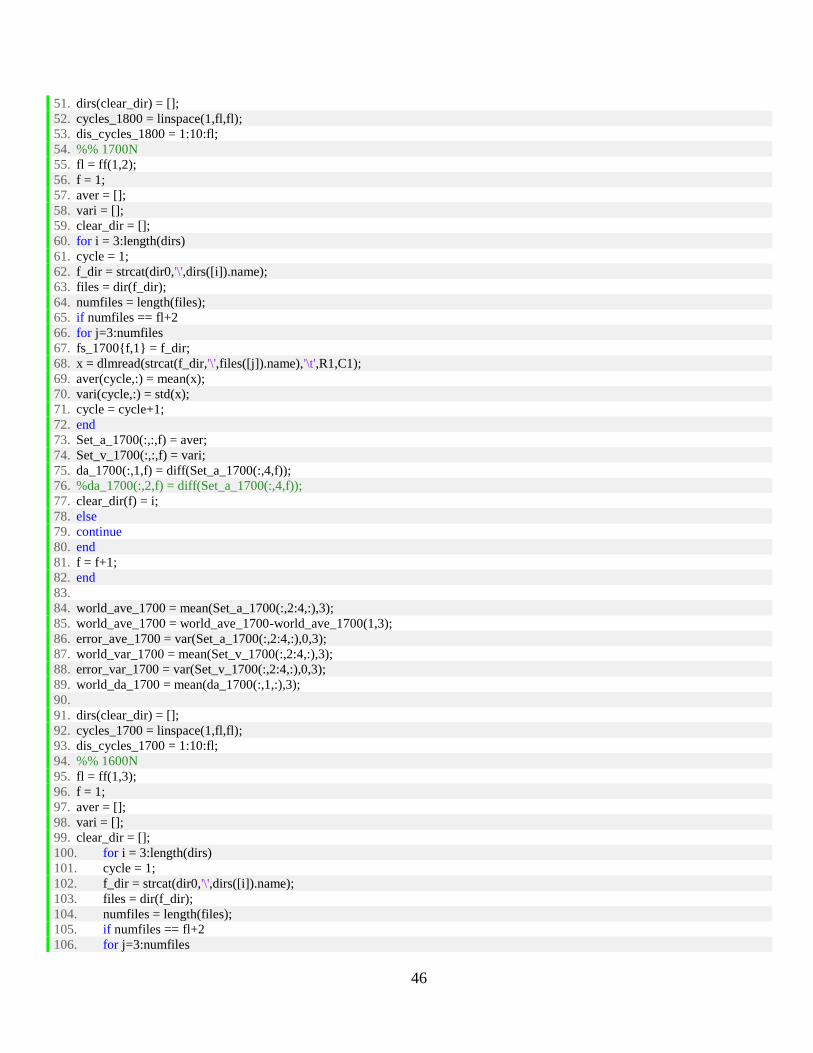
46

51. dirs(clear_dir) = [];

52. cycles_1800 = linspace(1,fl,fl);

53. dis_cycles_1800 = 1:10:fl;

54. %% 1700N

55. fl = ff(1,2);

56. f = 1;

57. aver = [];

58. vari = [];

59. clear_dir = [];

60. for i = 3:length(dirs)

61. cycle = 1;

62. f_dir = strcat(dir0,'\',dirs([i]).name);


64. numfiles = length(files);

65. if numfiles == fl+2

66. for j=3:numfiles

67. fs_1700{f,1} = f_dir;

68. x = dlmread(strcat(f_dir,'\',files([j]).name),'\t',R1,C1);

69. aver(cycle,:) = mean(x);

70. vari(cycle,:) = std(x);

71. cycle = cycle+1;

72. end

73. Set_a_1700(:,:,f) = aver;

74. Set_v_1700(:,:,f) = vari;

75. da_1700(:,1,f) = diff(Set_a_1700(:,4,f));

76. %da_1700(:,2,f) = diff(Set_a_1700(:,4,f));


78. else

79. continue

80. end

81. f = f+1;

82. end

83.






89. world_da_1700 = mean(da_1700(:,1,:),3);

90.



93. dis_cycles_1700 = 1:10:fl;

94. %% 1600N

95. fl = ff(1,3);

96. f = 1;

97. aver = [];

98. vari = [];

99. clear_dir = [];

100. for i = 3:length(dirs)

101. cycle = 1;

102. f_dir = strcat(dir0,'\',dirs([i]).name);


104. numfiles = length(files);

105. if numfiles == fl+2

106. for j=3:numfiles

47

107. fs_1600{f,1} = f_dir;

108. x = dlmread(strcat(f_dir,'\',files([j]).name),'\t',R1,C1);

109. aver(cycle,:) = mean(x);

110. vari(cycle,:) = std(x);

111. cycle = cycle+1;

112. end

113. Set_a_1600(:,:,f) = aver;

114. Set_v_1600(:,:,f) = vari;

115. da_1600(:,1,f) = diff(Set_a_1600(:,4,f));

116. %da_1600(:,2,f) = diff(Set_a_1600(:,4,f)); %Reads FEA calibation


118. else

119. continue

120. end

121. f = f+1;

122. end

123.






129. world_da_1600 = mean(da_1600(:,1,:),3);

130.



133. dis_cycles_1600 = 1:10:fl;

134.

135. %% 1400N


137. f = 1;

138. aver = [];

139. vari = [];













152. end



155. da_1400(:,1,f) = diff(Set_a_1400(:,4,f)); %calculate the difference between holding cycle averages for Johnson



158. else

159. continue

160. end


162. end

48

163.






169. world_da_1400 = mean(da_1400(:,1,:),3);

170.

171. dirs(clear_dir(1,f-1)) = [];


173. dis_cycles_1400 = 1:20:fl;

174.

175. %% 1200N


177. f = 1;

178. aver = [];

179. vari = [];













192. end






198. else

199. continue

200. end


202. end

203.






209. world_da_1200 = mean(da_1200(:,1,:),3);

210.

211. dirs(clear_dir(1,f-1)) = [];


213. dis_cycles_1200 = 1:50:fl;

214.

215. %% 1000N


217. f = 1;

218. aver = [];

49

219. vari = [];













232. end






238. else

239. continue

240. end


242. end

243.






249. world_da_1000 = mean(da_1000(:,1,:),3);

250.

251. dirs(clear_dir(1,f-1)) = [];


253. dis_cycles_1000 = 1:50:fl;

254.

255. %%

256. a_1000 = Set_a_1000(:,3,:)*10^-3;

257. a_1000_ave = mean(a_1000,3);

258. a_1200 = Set_a_1200(:,3,:)*10^-3;

259. a_1200_ave = mean(a_1200,3);

260. a_1400 = Set_a_1400(:,3,:)*10^-3;

261. a_1400_ave = mean(a_1400,3);

262. a_1600 = Set_a_1600(:,3,:)*10^-3; %Crack length from load line to tip in m

263. a_1600_ave = mean(a_1600,3); %Crack length average across all samples in m

264. a_1700 = Set_a_1700(:,3,:)*10^-3;

265. a_1700_ave = mean(a_1700,3);

266. a_1800 = Set_a_1800(:,3,:)*10^-3;

267. a_1800_ave = mean(a_1800,3);

268.

269. %% Stress Intensity

270. a0 = 10*10^-3; %Length of initial crack in m

271. w = 34.25*10^-3; %Width of sample in m

272. h = 76.2*10^-3; %Height of sample in m

273. t = 0.5*10^-3; %Thickenss of sample in m

274.

50

275. P_max_1000 = Set_a_1000(:,2,:);

276. P_min_1000 = 255;

277. K_I_max_1000 = (P_max_1000./(t.*(w)))*10^-6.*sqrt(pi().*a_1000).*(8.574-10.365*(a_1000/w)+5.499*(a_1000/w).^2);

278. K_I_min_1000 = (P_min_1000./(t.*(w)))*10^-6.*sqrt(pi().*a_1000).*(8.574-10.365.*(a_1000./w)+5.499.*(a_1000./w).^2);

279. dK_I_1000 = K_I_max_1000-K_I_min_1000;

280. dK_I_ave_1000 = mean(dK_I_1000,3);

281. P_max_1200 = Set_a_1200(:,2,:);

282. P_min_1200 = 180;

283. K_I_max_1200 = (P_max_1200./(t.*(w)))*10^-6.*sqrt(pi().*a_1200).*(8.574-10.365*(a_1200./w)+5.499*(a_1200./w).^2);

284. K_I_min_1200 = (P_min_1200./(t.*(w)))*10^-6.*sqrt(pi().*a_1200).*(8.574-10.365*(a_1200./w)+5.499*(a_1200./w).^2);

285. dK_I_1200 = K_I_max_1200-K_I_min_1200;

286. dK_I_ave_1200 = mean(dK_I_1200,3);

287. P_max_1400 = Set_a_1400(:,2,:);

288. P_min_1400 = 195;


290. K_I_min_1400 = (P_min_1400./(t.*(w)))*10^-6.*sqrt(pi().*a_1400).*(8.574-10.365*(a_1400/w)+5.499*(a_1400/w).^2);

291. dK_I_1400 = K_I_max_1400-K_I_min_1400;

292. dK_I_ave_1400 = mean(dK_I_1400,3);

293. P_max_1600 = Set_a_1600(:,2,:);

294. P_min_1600 = 207.8;



297. dK_I_1600 = K_I_max_1600-K_I_min_1600;

298. dK_I_ave_1600 = mean(dK_I_1600,3);

299. P_max_1700 = Set_a_1700(:,2,:);

300. P_min_1700 = 227.8;



303. dK_I_1700 = K_I_max_1700-K_I_min_1700;

304. dK_I_ave_1700 = mean(dK_I_1700,3);

305. P_max_1800 = Set_a_1800(:,2,:);

306. P_min_1800 = 253.26;

307. K_I_max_1800 = ((P_max_1800/(t*w))*10^-6).*sqrt(pi().*a_1800).*(8.574-10.365*(a_1800/w)+5.499*(a_1800/w).^2);

308. K_I_min_1800 = ((P_min_1800/(t*w))*10^-6).*sqrt(pi().*a_1800).*(8.574-10.365*(a_1800/w)+5.499*(a_1800/w).^2);

309. dK_I_1800 = K_I_max_1800-K_I_min_1800;

310. dK_I_ave_1800 = mean(dK_I_1800,3);

311.

312. %% Saving Data

313. cd 'Matlab Variables'\

314.

315. save('Data_Collect.mat')

316.

317. cd ..

51

Appendix D: Matlab Plotting Script

1. %% File Initialization

2. clc,close all

3.

4. cd 'Matlab Variables'\

5.

6. load('Data_Collect.mat')

7.

8. cd ..

9.

10. a_1000(2012) = [];

11. dK_I_1000(2012) = [];

12.

13. %%

14. bins = 20;

15. num_1000 = size(cycles_1000,2);

16. num_1200 = size(cycles_1200,2);

17. num_1400 = size(cycles_1400,2);

18. num_1600 = size(cycles_1600,2);

19. num_1700 = size(cycles_1700,2);

20. num_1800 = size(cycles_1800,2);

21.

22. xy1 = linspace(-0.08,0.08,1000);

23. xy2 = linspace(-0.02,0.02,1000);

24.

25. samp_num = [size(dK_I_1000,3),size(dK_I_1200,3),size(dK_I_1400,3),size(dK_I_1600,3),size(dK_I_1700,3),size(dK_I_1800,3)];

26. samp_num_str =

{num2str(size(dK_I_1000,3)),num2str(size(dK_I_1200,3)),num2str(size(dK_I_1400,3)),num2str(size(dK_I_1600,3)),num2str(size(

dK_I_1700,3)),num2str(size(dK_I_1800,3))};

27.

28. %% Average Crack Length vs Cycle Plot - Semilog plot

29. figure('units','normalized','outerposition',[0.25,0.25,0.5,0.75]);

30. semilogx(dis_cycles_1000,world_ave_1000(dis_cycles_1000,3),'LineWidth',1.5,'color','magenta')

31. hold on; semilogx(dis_cycles_1200,world_ave_1200(dis_cycles_1200,3),'LineWidth',1.5,'color','black')

32. hold on; semilogx(dis_cycles_1400,world_ave_1400(dis_cycles_1400,3),'LineWidth',1.5,'color','cyan')

33. hold on; semilogx(dis_cycles_1600,world_ave_1600(dis_cycles_1600,3),'LineWidth',1.5,'color','green')

34. hold on; semilogx(dis_cycles_1700,world_ave_1700(dis_cycles_1700,3),'LineWidth',1.5,'color','red')

35. hold on;semilogx(dis_cycles_1800,world_ave_1800(dis_cycles_1800,3),'LineWidth',1,'color','blue')

36.

37. legen = {'F_{max} = 1000N, n=','F_{max} = 1200N, n=','F_{max} = 1400N, n=','F_{max} = 1600N, n=','F_{max} = 1700N,

n=','F_{max} = 1800N, n='};

38. legen = strcat(legen,samp_num_str);

39. grid on

40. xlabel('Loading Cycle','FontSize',18,'FontWeight','bold') %Sets name, font size, and makes the font bold

41. ylabel('Crack Length [mm]','FontSize',18,'FontWeight','bold') %Sets name, font size, and makes the font bold

42. axis([0, 4500, 0, 2]);

43. leg=legend(legen);

44. legend('Location','northwest')

45. pbaspect([1 1 1]) %Makes the plot square

46. box(gca,'on') %Turns outside border on

47. set(gca,'LineWidth',3) %Creates a thick outside border

48. set(gca,'FontSize',18) %Sets Axis Font Size for number, can't make to big

49. set(leg,'FontSize',14) %Sets Legend Font Size

52

50. set(gca,'fontname','Times New Roman')

51. cd Figures\;saveas(gcf,'Fig4','epsc');saveas(gcf,'Fig4','tiffn');cd ..

52.

53. %% Non-Demensionalized Histogram plot

54.

55. t1 = world_da_1600./(((16.7.*(a_1600_ave(2:end)/0.03463).^(1/2)-

104.7.*(a_1600_ave(2:end)/0.03463).^(3/2)+369.9.*(a_1600_ave(2:end)/0.03463).^(5/2)-

573.8.*(a_1600_ave(2:end)/0.03463).^(7/2)+360.5.*(a_1600_ave(2:end)/0.03463).^(9/2)))...

/(16.7*(0.01/0.03463)^(1/2)-104.7*(0.01/0.03463)^(3/2)+369.9*(0.01/0.03463)^(5/2)-

573.8*(0.01/0.03463)^(7/2)+360.5*(0.01/0.03463)^(9/2)));


104.7.*(a_1700_ave(2:end)/0.03463).^(3/2)+369.9.*(a_1700_ave(2:end)/0.03463).^(5/2)-

573.8.*(a_1700_ave(2:end)/0.03463).^(7/2)+360.5.*(a_1700_ave(2:end)/0.03463).^(9/2)))...

/(16.7*(0.01/0.03463)^(1/2)-104.7*(0.01/0.03463)^(3/2)+369.9*(0.01/0.03463)^(5/2)-

573.8*(0.01/0.03463)^(7/2)+360.5*(0.01/0.03463)^(9/2)));


104.7.*(a_1800_ave(2:end)/0.03463).^(3/2)+369.9.*(a_1800_ave(2:end)/0.03463).^(5/2)-

573.8.*(a_1800_ave(2:end)/0.03463).^(7/2)+360.5.*(a_1800_ave(2:end)/0.03463).^(9/2)))...

/(16.7*(0.01/0.03463)^(1/2)-104.7*(0.01/0.03463)^(3/2)+369.9*(0.01/0.03463)^(5/2)-

573.8*(0.01/0.03463)^(7/2)+360.5*(0.01/0.03463)^(9/2)));


104.7.*(a_1400_ave(2:end)/0.03463).^(3/2)+369.9.*(a_1400_ave(2:end)/0.03463).^(5/2)-

573.8.*(a_1400_ave(2:end)/0.03463).^(7/2)+360.5.*(a_1400_ave(2:end)/0.03463).^(9/2)))...

/(16.7*(0.01/0.03463)^(1/2)-104.7*(0.01/0.03463)^(3/2)+369.9*(0.01/0.03463)^(5/2)-

573.8*(0.01/0.03463)^(7/2)+360.5*(0.01/0.03463)^(9/2)));


104.7.*(a_1200_ave(2:end)/0.03463).^(3/2)+369.9.*(a_1200_ave(2:end)/0.03463).^(5/2)-

573.8.*(a_1200_ave(2:end)/0.03463).^(7/2)+360.5.*(a_1200_ave(2:end)/0.03463).^(9/2)))...

/(16.7*(0.01/0.03463)^(1/2)-104.7*(0.01/0.03463)^(3/2)+369.9*(0.01/0.03463)^(5/2)-

573.8*(0.01/0.03463)^(7/2)+360.5*(0.01/0.03463)^(9/2)));


104.7.*(a_1000_ave(2:end)/0.03463).^(3/2)+369.9.*(a_1000_ave(2:end)/0.03463).^(5/2)-

573.8.*(a_1000_ave(2:end)/0.03463).^(7/2)+360.5.*(a_1000_ave(2:end)/0.03463).^(9/2)))...

/(16.7*(0.01/0.03463)^(1/2)-104.7*(0.01/0.03463)^(3/2)+369.9*(0.01/0.03463)^(5/2)-

573.8*(0.01/0.03463)^(7/2)+360.5*(0.01/0.03463)^(9/2)));

61.

62. t1 = movmean(t1,10);

63. t2 = movmean(t2,10);

64. t3 = movmean(t3,10);

65. t4 = movmean(t4,10);

66. t5 = movmean(t5,10);

67. t6 = movmean(t6,10);

68. stand_t1 = std(t1);






74. c = [0.75, 0.75, 0.75];

75.

76. %1600N


78. hold on; subplot(1,3,2:3); plot(t1,'LineWidth',1,'color','green')%errorbar at 5% VL, width calcuated using a t distributiongrid on

79. grid on; grid minor; set(gca,'YminorTick','on')

80. xlabel('Loading Cycle','FontSize',18,'FontWeight','bold')%Sets name, font size, and makes the font bold

53

81. ylim([-0.2*max(t1), max(t1)+0.1*max(t1)]);% xlim([-1.05, 420]);

82. yl = ylim;

83. leg=legend('F_{max} = 1600N');

84. legend('Location','southeast')






90. pbaspect([1 0.75 1])

91.

92. xy2 = linspace(-max(t1),max(t1),1000);

93. subplot(1,3,1);

94. pdf1 = normpdf(xy2,0,stand_t1);

95. hold on; patch(pdf1/3,xy2,c);

96. h1 = histogram(t1,bins,'Orientation','horizontal');

97. h1(1).FaceColor = 'g';


99. set(get(get(h1,'Annotation'),'LegendInformation'),'IconDisplayStyle','off');

100. h = gca;

101. xl = xlim;

102. set(h,'XDir','reverse');

103. xlabel('Count','FontSize',18,'FontWeight','bold') %Sets name, font size, and makes the font bold

104. ylabel('\Deltaa/\DeltaN(K_{0}/K(a)) [mm/cycle]','FontSize',18,'FontWeight','bold') %Sets name, font size, and makes the font bold

105. h.YLim = yl; h.XLim = [-1.5 xl(2)+10];

106. leg=legend('Normal Dist.');

107. legend('Location','southwest')






113. pbaspect([1.5 2.6 1])


115. 116. %1700N


118. hold on; subplot(1,3,2:3); plot(t2,'LineWidth',1,'color','red') %errorbar at 5% VL, width calcuated using a t distribution




122. yl = ylim;








130. pbaspect([1 0.75 1])

131. 132. xy2 = linspace(-max(t2),max(t2),1000);

133. subplot(1,3,1);



136. h2 = histogram(t2,bins, 'Orientation','horizontal');

54

137. h2(1).FaceColor = 'r';


139. xl = xlim;


141. h = gca;

142. xl = xlim;




146. h.YLim = yl; h.XLim = [-1.05 xl(2)+10];








154. pbaspect([1.5 2.6 1])


156. 157. %1800N


159. hold on; subplot(1,3,2:3); plot(t3,'LineWidth',1,'color','blue') %errorbar at 5% VL, width calcuated using a t distribution




163. yl = ylim;








171. pbaspect([1 0.75 1])


174. subplot(1,3,1);



177. h3 = histogram(t3,bins, 'Orientation','horizontal');

178. h3(1).FaceColor = 'b';


180. xl = xlim;


182. h = gca;




186. h.YLim = yl; h.XLim = [-0.5 xl(2)+10];







55


194. pbaspect([1.5 2.6 1])


196. 197. %1400N


199. hold on; subplot(1,3,2:3); plot(t4,'LineWidth',1,'color','cyan')%errorbar at 5% VL, width calcuated using a t distributiongrid on



202. %ylim([-0.4*max(t4), max(t4)+0.1*max(t4)]);% xlim([-1.05, 420]);

203. yl = ylim;








211. pbaspect([1 0.75 1])


214. subplot(1,3,1);




218. h4(1).FaceColor = 'cyan';



221. h = gca;

222. xl = xlim;




226. h.YLim = yl; h.XLim = [-1.5 xl(2)+10];








234. pbaspect([1.5 2.6 1])


236. 237. %1200N


239. hold on; subplot(1,3,2:3); plot(t5,'LineWidth',1,'color','black')%errorbar at 5% VL, width calcuated using a t distributiongrid on



242. %ylim([-0.2*max(t4), max(t4)+0.1*max(t4)]);% xlim([-0.5, 2760]);

243. yl = ylim;






56



251. pbaspect([1 0.75 1])


254. subplot(1,3,1);


256. hold on; patch(pdf1*5,xy2,c);


258. h5(1).FaceColor = 'black';



261. h = gca;

262. xl = xlim;




266. h.YLim = yl; h.XLim = [-1.5 xl(2)+10];








274. pbaspect([1.5 2.6 1])


276. 277. %1000N


279. hold on; subplot(1,3,2:3); plot(t6,'LineWidth',1,'color','magenta')%errorbar at 5% VL, width calcuated using a t distributiongrid on



282. %ylim([-0.1, 0.1]); xlim([-0.5, 4500]);

283. yl = ylim;








291. pbaspect([1 0.75 1])


294. subplot(1,3,1);


296. hold on; patch(pdf1,xy2,c);


298. h6(1).FaceColor = 'magenta';



301. h = gca;

302. xl = xlim;



57


306. h.YLim = yl; h.XLim = [-1.5 xl(2)+10];








314. pbaspect([1.5 2.6 1])


316. 317. %% Combined Histogram plot


319. bin_size = range(t3)/15;

320. bin_c = round([range(t1)/bin_size range(t2)/bin_size range(t3)/bin_size range(t4)/bin_size range(t5)/bin_size range(t5)/bin_size]);

321. histogram(t6,bin_c(6),'Normalization','probability','FaceColor','magenta','EdgeColor','magenta','FaceAlpha',0.5);hold on;

322. histogram(t5,bin_c(5),'Normalization','probability','FaceColor','black','EdgeColor','black','FaceAlpha',0.5);hold on;

323. histogram(t4,bin_c(4),'Normalization','probability','FaceColor','cyan','EdgeColor','cyan','FaceAlpha',0.5);hold on;

324. histogram(t1,bin_c(1),'Normalization','probability','FaceColor','blue','EdgeColor','blue','FaceAlpha',0.5);hold on;

325. histogram(t2,bin_c(2),'Normalization','probability','FaceColor','red','EdgeColor','red','FaceAlpha',0.5);hold on;

326. histogram(t3,bin_c(3),'Normalization','probability','FaceColor','green','EdgeColor','green','FaceAlpha',0.5);

327. 328. grid on

329. xlabel('\Deltaa/\DeltaN(K_{0}/K(a)) [mm/cycle]','FontSize',18,'FontWeight','bold')

330. ylabel('Probability','FontSize',18,'FontWeight','bold')

331. legend(legen,'location','northwest')

332. pbaspect([1 1 1])

333. box(gca,'on')

334. %set(gca,'YScale','log')


336. set(gca,'FontSize',18)


338. cd Figures\;saveas(gcf,'Figx','epsc');saveas(gcf,'Figx','tiffn');cd ..

339. 340. %% da/dn scatter plot

341. 342. figure('units','normalized','outerposition',[0.25,0.25,0.5,0.75]);

343. for i = 1:max(samp_num) %For all samples

344. if i <= samp_num(1)

345. hold on;y1 = scatter(dK_I_1000(:,:,i),a_1000(:,:,i),'magenta','filled');

346. end;if i <= samp_num(2)

347. hold on;y2 = scatter(dK_I_1200(:,:,i),a_1200(:,:,i),'black','filled');


349. hold on;y3 = scatter(dK_I_1400(:,:,i),a_1400(:,:,i),'cyan','filled');


351. hold on;y4 = scatter(dK_I_1600(:,:,i),a_1600(:,:,i),'green','filled');


353. hold on;y5 = scatter(dK_I_1700(:,:,i),a_1700(:,:,i),'red','filled');


355. hold on;y6 = scatter(dK_I_1800(:,:,i),a_1800(:,:,i),'blue','filled');

356. end

357. end

358. triang_x = [20 30];

359. triang_y = interp1(dK_I_1800(:,:,1), a_1800(:,:,1), triang_x);

360. slope = diff(triang_y)/diff(triang_x);

58

361. loglog(triang_x([1,2,2]),triang_y([1,1,2]),'k','LineWidth',4)

362. txt = 'm';

363. text(mean(triang_x),(triang_y(1)-0.15*triang_y(1)),txt,'FontSize',18,'FontWeight','bold')

364. grid on

365. xlabel('\DeltaK [MPa\surdm]','FontSize',26,'FontWeight','bold') %Sets name, font size, and makes the font bold

366. ylabel('\Deltaa/\DeltaN [mm/cycle]','FontSize',26,'FontWeight','bold') %Sets name, font size, and makes the font bold

367. xlim([2 80]);

368. leg=legend('F_{max} = 1000N','F_{max} = 1200N','F_{max} = 1400N','F_{max} = 1600N','F_{max} = 1700N','F_{max} =

1800N');

369. legend('Location','northwest')

370. pbaspect([1 1 1]) %Makes the plot square






376. set(gca,'XScale','log')

377. set(gca,'YScale','log')


IN SITU MEASUREMENT OF FATIGUE INDUCED CRACK GROWTH …

Documents

Transcript of IN SITU MEASUREMENT OF FATIGUE INDUCED CRACK GROWTH …