1 Pertemuan 06 Sebaran Normal dan Sampling Matakuliah: >K0614/ >FISIKA Tahun: >2006.

1

Pertemuan 06

Sebaran Normal dan Sampling

Matakuliah : <<Kode>>K0614/<<Nama mtkul>>FISIKA

Tahun : <<Tahun Pembuatan>>2006

2

Outline Materi:

• Peluang sebaran normal

• Sebaran rata-rata sampling

• Sebaran proporsi sampling

3

Basic Business Statistics (9th Edition)

The Normal Distribution and Other Continuous

Distributions

4

Peluang sebaran normal

• The Normal Distribution

• The Standardized Normal Distribution

• Evaluating the Normality Assumption

• The Uniform Distribution

• The Exponential Distribution

5

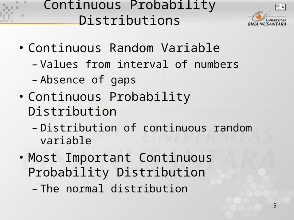
Continuous Probability Distributions

• Continuous Random Variable– Values from interval of numbers– Absence of gaps

• Continuous Probability Distribution– Distribution of continuous random variable

• Most Important Continuous Probability Distribution– The normal distribution

6

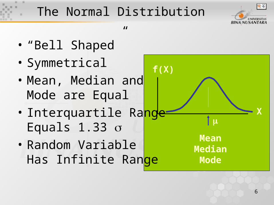
The Normal Distribution

• “Bell Shaped”

• Symmetrical

• Mean, Median and Mode are Equal

• Interquartile RangeEquals 1.33

• Random VariableHas Infinite Range

Mean Median Mode

X

f(X)

7

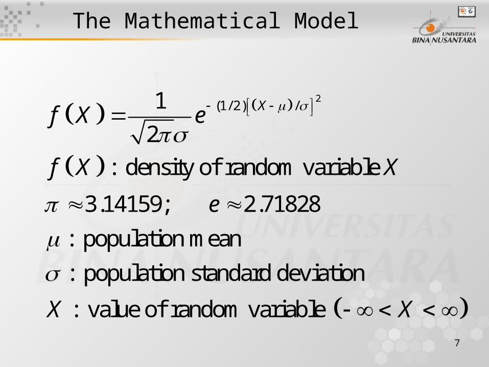
The Mathematical Model

2(1/ 2) /1

2

: density of random variable

3.14159; 2.71828

: population mean

: population standard deviation

: value of random variable

Xf X e

f X X

e

X X

8

Many Normal Distributions

Varying the Parameters and , We Obtain Different Normal Distributions

There are an Infinite Number of Normal Distributions

9

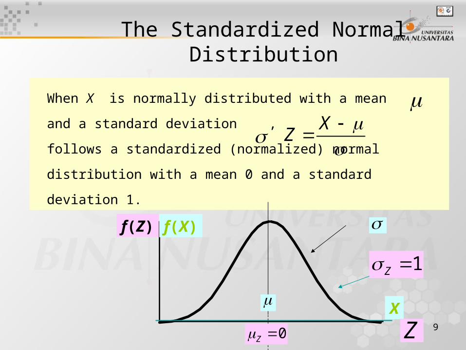
The Standardized Normal Distribution

When X is normally distributed with a mean and

a standard deviation , follows a

standardized (normalized) normal distribution with a

mean 0 and a standard deviation 1.

XZ

X

f(X)

Z

0Z

1Z

f(Z)

10

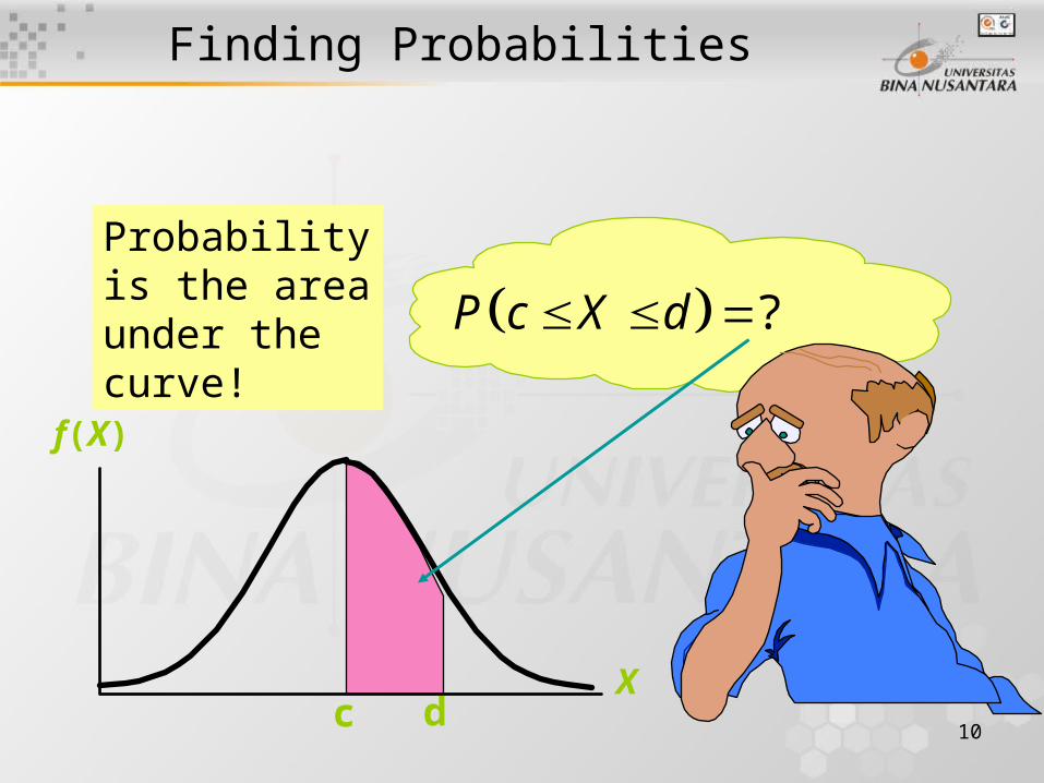
Finding Probabilities

Probability is the area under the curve!

c dX

f(X)

?P c X d

11

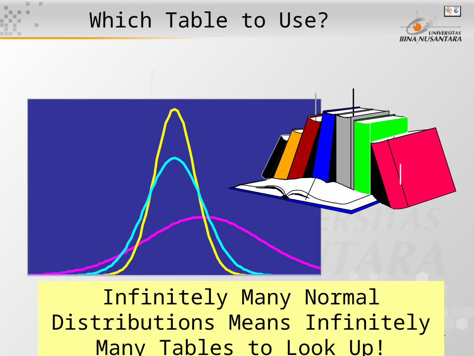
Which Table to Use?

Infinitely Many Normal Distributions Means Infinitely Many Tables to Look

Up!

12

Solution: The Cumulative Standardized Normal Distribution

Z .00 .01

0.0 .5000 .5040 .5080

.5398 .5438

0.2 .5793 .5832 .5871

0.3 .6179 .6217 .6255

.5478.02

0.1 .5478

Cumulative Standardized Normal Distribution Table (Portion)

Probabilities

Only One Table is Needed

0 1Z Z

Z = 0.12

0

13

Standardizing Example

6.2 50.12

10

XZ

Normal Distribution

Standardized Normal

Distribution10 1Z

5 6.2 X Z

0Z 0.12

14

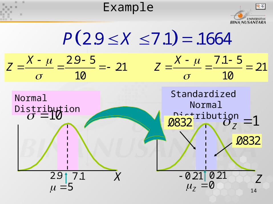
Example

Normal Distribution

Standardized Normal

Distribution10 1Z

5 7.1 X Z0Z

0.21

2.9 5 7.1 5.21 .21

10 10

X XZ Z

2.9 0.21

.0832

2.9 7.1 .1664P X

.0832

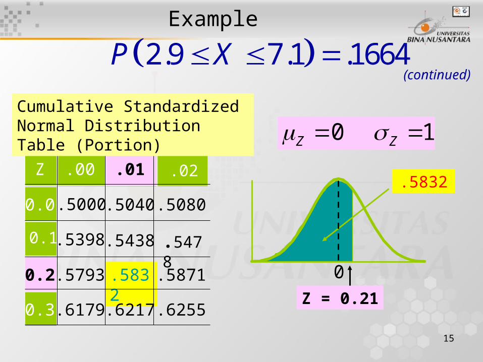
15

Z .00 .01

0.0 .5000 .5040 .5080

.5398 .5438

0.2 .5793 .5832 .5871

0.3 .6179 .6217 .6255

.5832.02

0.1 .5478


0 1Z Z

Z = 0.21

Example

2.9 7.1 .1664P X (continued)

0

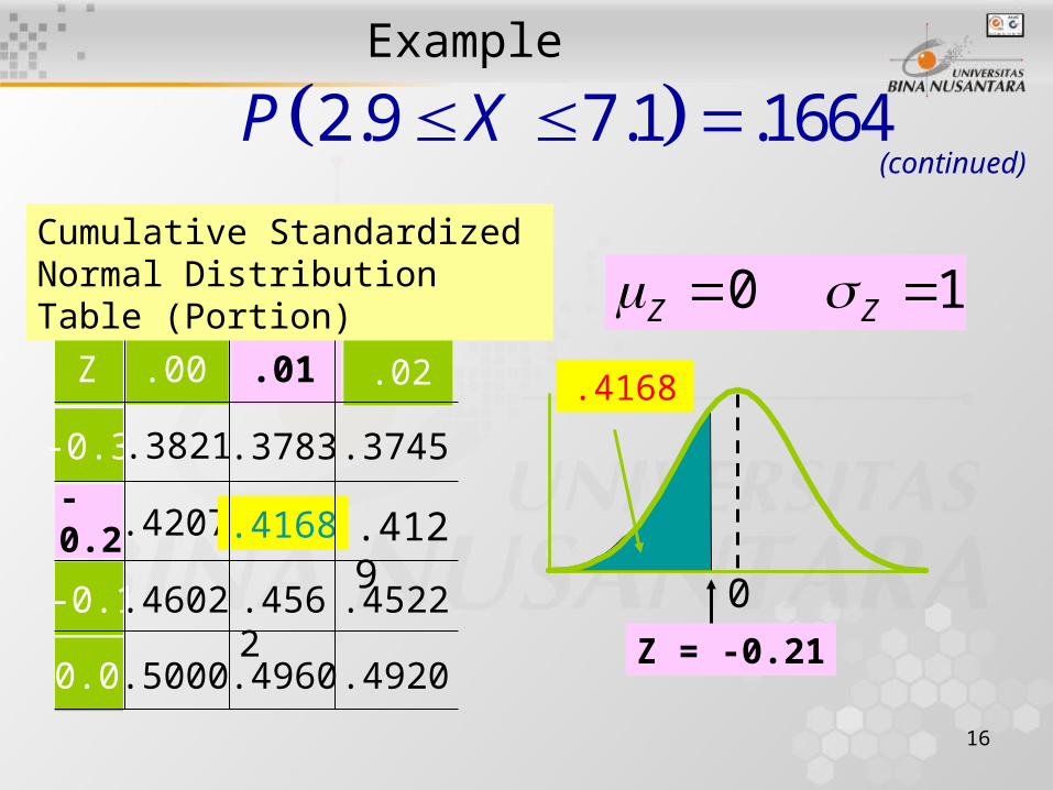
16

Z .00 .01

-0.3 .3821 .3783 .3745

.4207 .4168

-0.1.4602 .4562 .4522

0.0 .5000 .4960 .4920

.4168.02

-0.2 .4129


0 1Z Z

Z = -0.21

Example

2.9 7.1 .1664P X (continued)

0

17

Normal Distribution in PHStat

• PHStat | Probability & Prob. Distributions | Normal …

• Example in Excel Spreadsheet

Microsoft Excel Worksheet

18

Example :

8 .3821P X

Normal Distribution

Standardized Normal

Distribution10 1Z

5 8 X Z0Z

0.30

8 5.30

10

XZ

.3821

19

Example:

Example:

8 .3821P X (continued)

Z .00 .01

0.0 .5000 .5040 .5080

.5398 .5438

0.2 .5793 .5832 .5871

0.3 .6179 .6217 .6255

.6179.02

0.1 .5478


0 1Z Z

Z = 0.30

0

20

.6217

Finding Z Values for Known Probabilities

Z .00 0.2

0.0 .5000 .5040 .5080

0.1 .5398 .5438 .5478

0.2 .5793 .5832 .5871

.6179 .6255

.01

0.3

Cumulative Standardized Normal Distribution Table

(Portion)

What is Z Given Probability = 0.6217 ?

.6217

0 1Z Z

.31Z 0

21

Recovering X Values for Known Probabilities

5 .30 10 8X Z

Normal Distribution

Standardized Normal

Distribution10 1Z

5 ? X Z0Z 0.30

.3821.6179

22

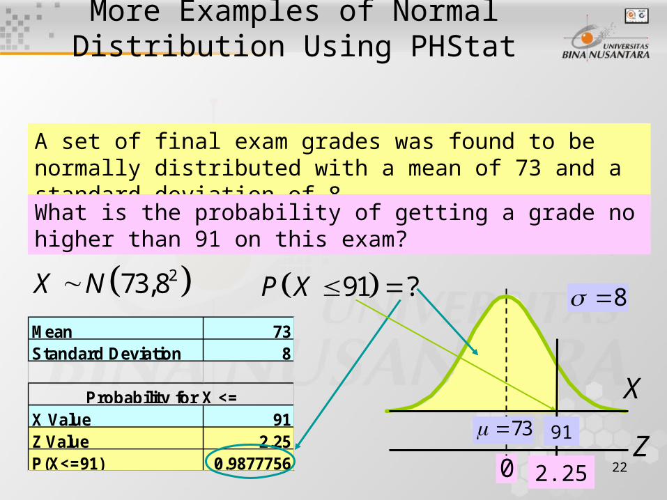
More Examples of Normal Distribution Using PHStat

A set of final exam grades was found to be normally distributed with a mean of 73 and a standard deviation of 8.What is the probability of getting a grade no higher than 91 on this exam?

273,8X N 91 ?P X Mean 73Standard Deviation 8

X Value 91Z Value 2.25P(X<=91) 0.9877756

Probability for X <=

2.250

X

Z91

8

73

23

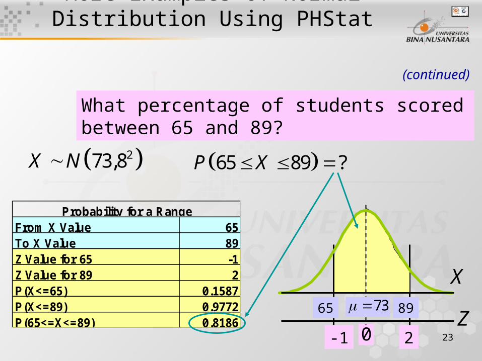
What percentage of students scored between 65 and 89?

From X Value 65To X Value 89Z Value for 65 -1Z Value for 89 2P(X<=65) 0.1587P(X<=89) 0.9772P(65<=X<=89) 0.8186

Probability for a Range

273,8X N 65 89 ?P X

20

X

Z8965

-1

73


(continued)

24

73

Only 5% of the students taking the test scored higher than what grade?

273,8X N ? .05P X

Cumulative Percentage 95.00%Z Value 1.644853X Value 86.15882

Find X and Z Given Cum. Pctage.

1.6450

X

Z? =86.16

(continued)


25

Assessing Normality

• Not All Continuous Random Variables are Normally Distributed

• It is Important to Evaluate How Well the Data Set Seems to Be Adequately Approximated by a Normal Distribution

26

Assessing Normality

• Construct Charts– For small- or moderate-sized data sets, do the

stem-and-leaf display and box-and-whisker plot look symmetric?

– For large data sets, does the histogram or polygon appear bell-shaped?

• Compute Descriptive Summary Measures– Do the mean, median and mode have similar

values?– Is the interquartile range approximately 1.33 ?– Is the range approximately 6 ?

(continued)

27

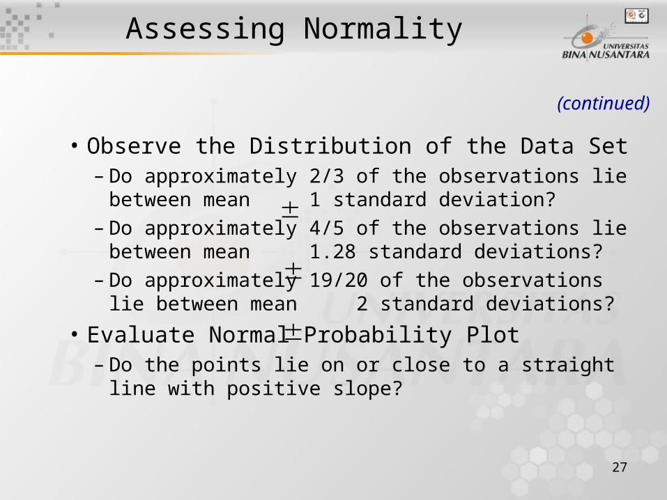
Assessing Normality

• Observe the Distribution of the Data Set– Do approximately 2/3 of the observations lie

between mean 1 standard deviation?– Do approximately 4/5 of the observations lie

between mean 1.28 standard deviations?– Do approximately 19/20 of the observations lie

between mean 2 standard deviations?

• Evaluate Normal Probability Plot– Do the points lie on or close to a straight line

with positive slope?

(continued)

28

Assessing Normality

• Normal Probability Plot– Arrange Data into Ordered Array– Find Corresponding Standardized Normal

Quantile Values– Plot the Pairs of Points with Observed Data

Values on the Vertical Axis and the Standardized Normal Quantile Values on the Horizontal Axis

– Evaluate the Plot for Evidence of Linearity

(continued)

29

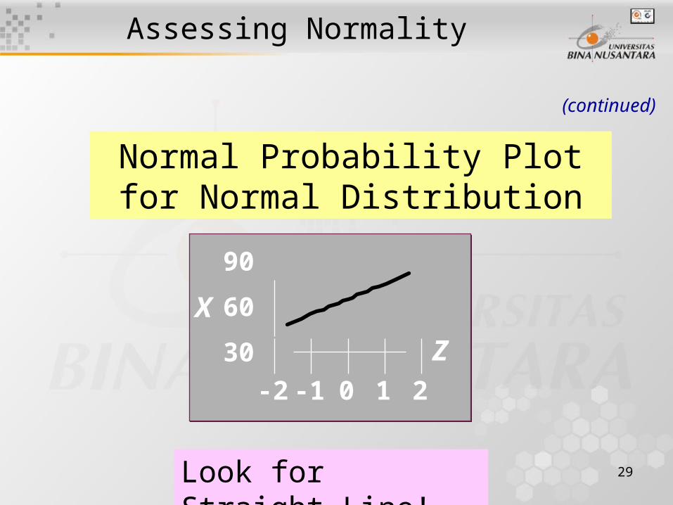
Assessing Normality

Normal Probability Plot for Normal Distribution

Look for Straight Line!

30

60

90

-2 -1 0 1 2

Z

X

(continued)

30

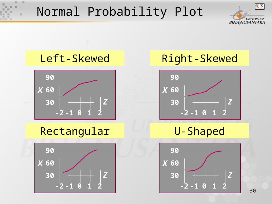
Normal Probability Plot

Left-Skewed Right-Skewed

Rectangular U-Shaped

30

60

90

-2 -1 0 1 2

Z

X

30

60

90

-2 -1 0 1 2

Z

X

30

60

90

-2 -1 0 1 2

Z

X

30

60

90

-2 -1 0 1 2

Z

X

31

Sampling Distribution

• Sampling Distribution of the Mean

• The Central Limit Theorem

• Sampling Distribution of the Proportion

• Sampling from Finite Population

32

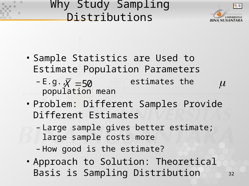
Why Study Sampling Distributions

• Sample Statistics are Used to Estimate Population Parameters– E.g., estimates the population mean

• Problem: Different Samples Provide Different Estimates– Large sample gives better estimate; large

sample costs more– How good is the estimate?

• Approach to Solution: Theoretical Basis is Sampling Distribution

50X

33


• Theoretical Probability Distribution of a Sample Statistic

• Sample Statistic is a Random Variable– Sample mean, sample proportion

• Results from Taking All Possible Samples of the Same Size

34

Developing Sampling Distributions

• Suppose There is a Population …

• Population Size N=4

• Random Variable, X,

is Age of Individuals

• Values of X: 18, 20,

22, 24 Measured in

YearsA

B C

D

35

1

2

1

18 20 22 2421

4

2.236

N

ii

N

ii

X

N

X

N

.3

.2

.1

0 A B C D (18) (20) (22) (24)

Uniform Distribution

P(X)

X


(continued)

Summary Measures for the Population Distribution

36

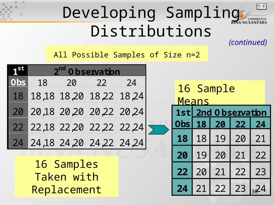
1st 2nd Observation Obs 18 20 22 24

18 18,18 18,20 18,22 18,24

20 20,18 20,20 20,22 20,24

22 22,18 22,20 22,22 22,24

24 24,18 24,20 24,22 24,24

All Possible Samples of Size n=2

16 Samples Taken with Replacement

16 Sample Means1st 2nd Observation Obs 18 20 22 24

18 18 19 20 21

20 19 20 21 22

22 20 21 22 23

24 21 22 23 24


(continued)

37

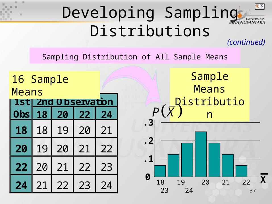
1st 2nd Observation Obs 18 20 22 24

18 18 19 20 21

20 19 20 21 22

22 20 21 22 23

24 21 22 23 24

Sampling Distribution of All Sample Means

18 19 20 21 22 23 240

.1

.2

.3

X

Sample Means

Distribution

16 Sample Means

_


(continued)

P X

38

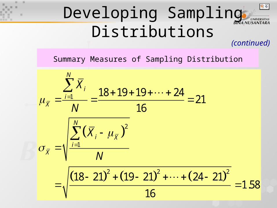
1

2

1

2 2 2

18 19 19 2421

16

18 21 19 21 24 211.58

16

N

ii

X

N

i Xi

X

X

N

X

N

Summary Measures of Sampling Distribution


(continued)

39

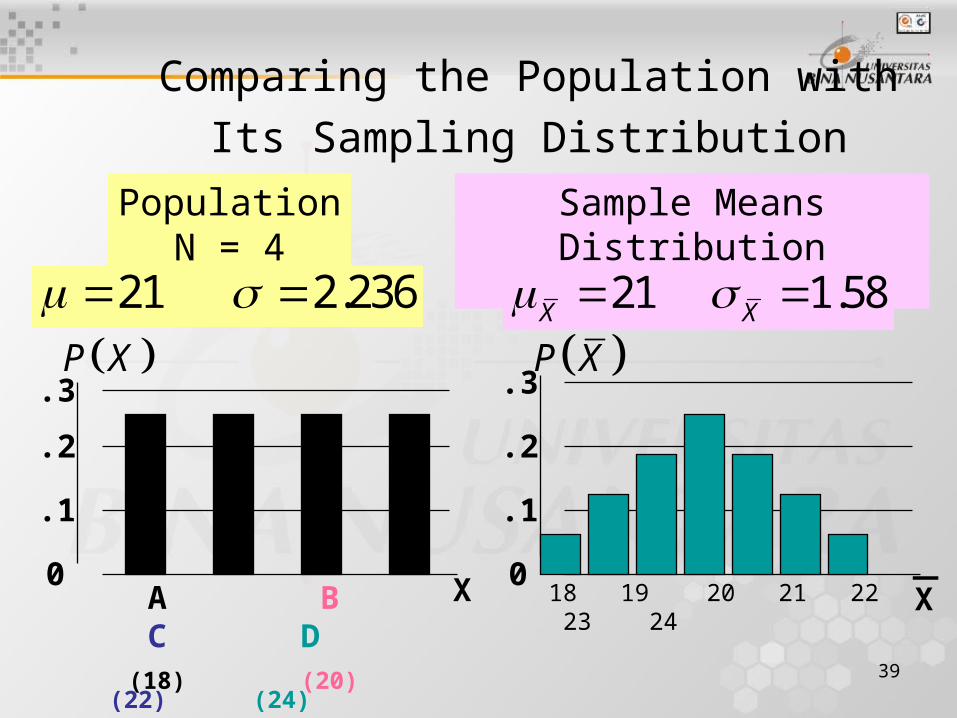
Comparing the Population with Its Sampling Distribution

18 19 20 21 22 23 240

.1

.2

.3

X

Sample Means Distribution

n = 2

A B C D (18) (20) (22) (24)

0

.1

.2

.3

PopulationN = 4

X_

21 2.236 21 1.58X X P X P X

40

Properties of Summary Measures

• – I.e., is unbiased

• Standard Error (Standard Deviation) of the Sampling Distribution is Less Than the Standard Error of Other Unbiased Estimators

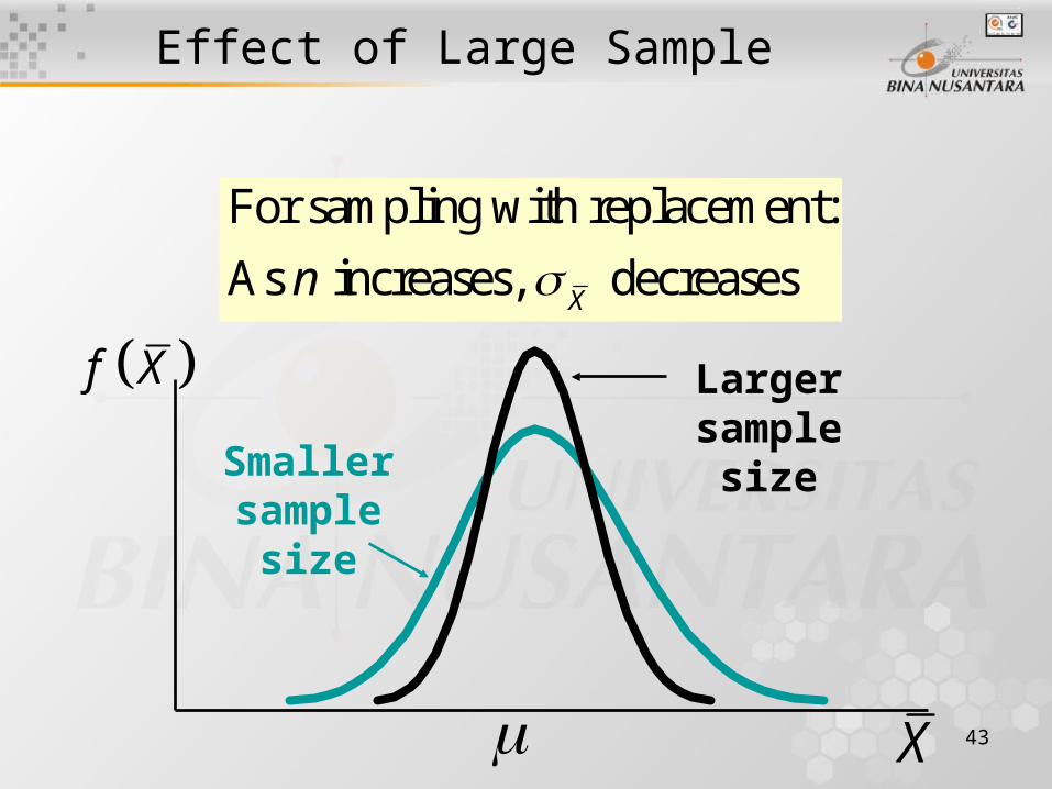
• For Sampling with Replacement or without Replacement from Large or Infinite Populations:

– As n increases, decreases

X

X

Xn

X

X

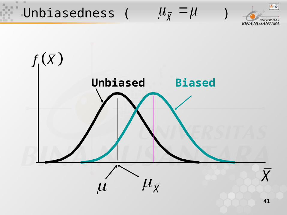
41

Unbiasedness ( )

BiasedUnbiased

X X

X

f X

42

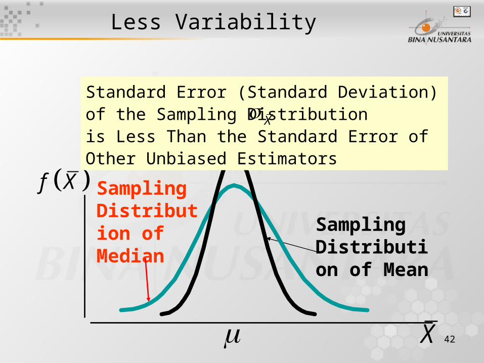
Less Variability

Sampling Distribution of Median Sampling

Distribution of Mean

X

f X

Standard Error (Standard Deviation) of the Sampling Distribution is Less Than the Standard Error of Other Unbiased Estimators

X

43

Effect of Large Sample

Larger sample size

Smaller sample size

X

f X

For sampling with replacement:

As increases, decreasesXn

44

When the Population is Normal

Central Tendency

Variation

Population Distribution

Sampling Distributions

X

Xn

X50X

4

5X

n

16

2.5X

n

50

10

45

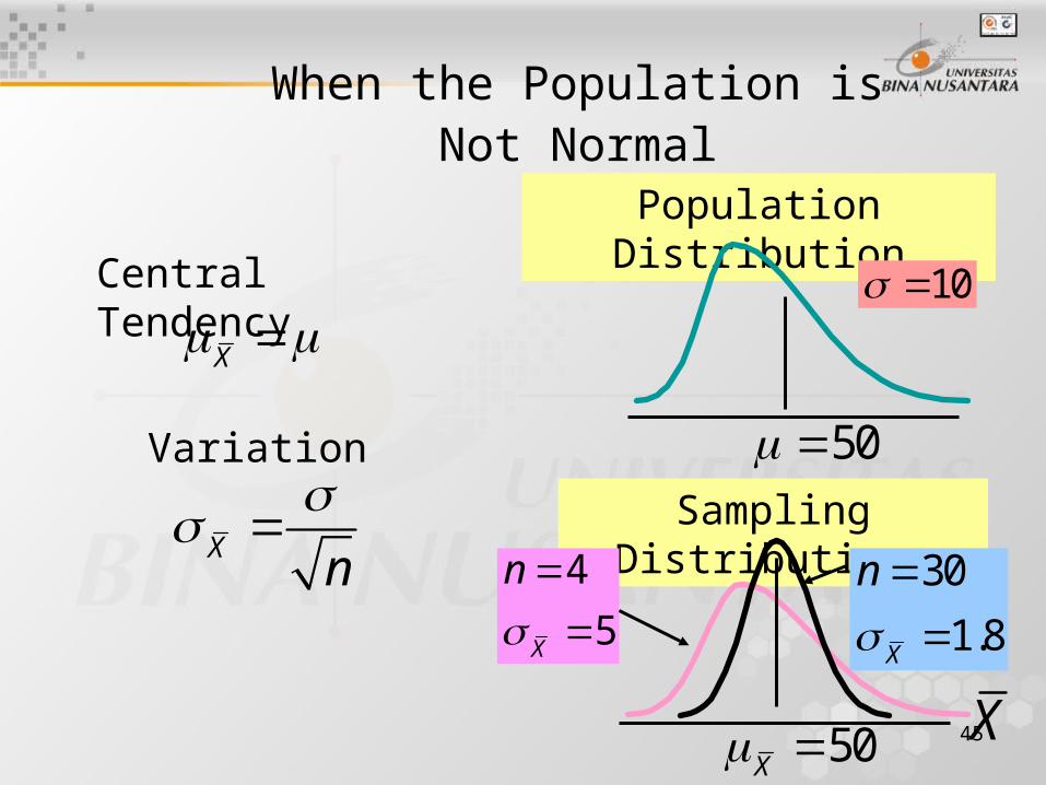
When the Population isNot Normal

Central Tendency

Variation

Population Distribution

Sampling Distributions

X

Xn

X50X

4

5X

n

30

1.8X

n

50

10

46

Central Limit Theorem

As Sample Size Gets Large Enough

Sampling Distribution Becomes Almost Normal Regardless of Shape of Population X

47

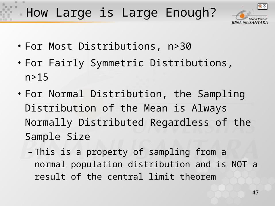
How Large is Large Enough?

• For Most Distributions, n>30

• For Fairly Symmetric Distributions, n>15

• For Normal Distribution, the Sampling

Distribution of the Mean is Always Normally

Distributed Regardless of the Sample Size

– This is a property of sampling from a normal

population distribution and is NOT a result of

the central limit theorem

48

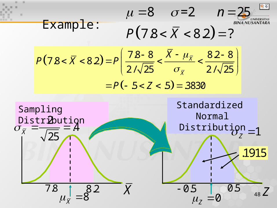
Example: 8 =2 25

7.8 8.2 ?

n

P X


Standardized Normal

Distribution2

.425

X 1Z

8X 8.2 Z0Z

0.5

7.8 8 8.2 87.8 8.2

2 / 25 2 / 25

.5 .5 .3830

X

X

XP X P

P Z

7.8 0.5

.1915

X

49

Population Proportions

• Categorical Variable

– E.g., Gender, Voted for Bush, College Degree

• Proportion of Population Having a Characteristic

• Sample Proportion Provides an Estimate

–

• If Two Outcomes, X Has a Binomial Distribution

– Possess or do not possess characteristic

number of successes

sample sizeS

Xp

n

p

p

50

Sampling Distribution ofSample Proportion

• Approximated by

Normal Distribution

–

– Mean:

•

– Standard error:

•

p = population proportion

Sampling Distributionf(ps)

.3

.2

.1 0

0 . 2 .4 .6 8 1ps

5np 1 5n p

Spp

1Sp

p p

n

51

Standardizing Sampling Distribution of Proportion

1S

S

S p S

p

p p pZ

p p

n


Standardized Normal

Distribution

Sp 1Z

Sp Sp Z0Z

52

Example:

200 .4 .43 ?Sn p P p

.43 .4.43 .87 .8078

.4 1 .4

200

S

S

S pS

p

pP p P P Z


Standardized Normal

DistributionSp

1Z

Sp

Sp Z0.43 .87

1 Pertemuan 06 Sebaran Normal dan Sampling Matakuliah: >K0614/ >FISIKA Tahun: >2006.

Documents

Transcript of 1 Pertemuan 06 Sebaran Normal dan Sampling Matakuliah: >K0614/ >FISIKA Tahun: >2006.