1 Flash Flood Detection in Urban Cities Using Ultrasonic...

Flash Flood Detection in Urban CitiesUsing Ultrasonic and Infrared Sensors

Item Type Article

Authors Mousa, Mustafa; Zhang, Xiangliang; Claudel, Christian

Citation Flash Flood Detection in Urban Cities Using Ultrasonic andInfrared Sensors 2016:1 IEEE Sensors Journal

Eprint version Post-print

DOI 10.1109/JSEN.2016.2592359

Publisher Institute of Electrical and Electronics Engineers (IEEE)

Journal IEEE Sensors Journal

Rights (c) 2016 IEEE. Personal use of this material is permitted.Permission from IEEE must be obtained for all other users,including reprinting/ republishing this material for advertising orpromotional purposes, creating new collective works for resaleor redistribution to servers or lists, or reuse of any copyrightedcomponents of this work in other works.

Download date 01/07/2018 06:52:02

Link to Item http://hdl.handle.net/10754/618396

http://dx.doi.org/10.1109/JSEN.2016.2592359

http://hdl.handle.net/10754/618396

1530-437X (c) 2016 IEEE. Personal use is permitted, but republication/redistribution requires IEEE permission. See http://www.ieee.org/publications_standards/publications/rights/index.html for more information.

This article has been accepted for publication in a future issue of this journal, but has not been fully edited. Content may change prior to final publication. Citation information: DOI 10.1109/JSEN.2016.2592359, IEEE SensorsJournal

1

Flash Flood Detection in Urban Cities UsingUltrasonic and Infrared Sensors

Mustafa Mousa*, Xiangliang Zhang* and Christian ClaudelΨ

*King Abdullah University of Science and TechnologyΨ The University of Texas at Austin

Abstract—Floods are the most common type of natural disaster.Often leading to loss of lives and properties in the thousandsyearly. Among these events, urban flash floods are particularlydeadly because of the short timescales on which they occur,and because of the population density of cities. Since most floodcasualties are caused by a lack of information on the impendingflood (type, location, severity), sensing these events is critical togenerate accurate and detailed warnings and short term forecasts.However, no dedicated flash flood sensing systems, that couldmonitor the propagation of flash floods, in real time, currentlyexist in cities. In the present paper, firstly a new sensing devicethat can simultaneously monitor urban flash floods and trafficcongestion has been presented. This sensing device is based on thecombination of ultrasonic range-finding with remote temperaturesensing, and can sense both phenomena with a high degree ofaccuracy, using a combination of L1-regularized reconstructionand artificial neural networks to process measurement data.Secondly, corresponding algorithms have been implemented ona low-power wireless sensor platform, and their performance inwater level estimation in a 6 months test involving four differentsensors is illustrated. The results demonstrate that urban waterlevels can be reliably estimated with error less than 2 cm, andthat the preprocessing and machine learning schemes can run inreal-time on currently available wireless sensor platforms.

Keywords—Water Level Estimation, ARMAX, Nonlinear Regres-sion, Artificial Neural Networks, Flood Detection.

I. INTRODUCTION

Wireless sensor networks (WSNs) are widely used formonitoring and control applications [1], [2], [3], [4], [5], [6]such as environmental surveillance [7], [8] or industrial sensing[9], or in the present case, flash flood detection. Floods areone of the most commonly occurring natural disasters [10],accounting for more than half of natural disasters worldwide.They have caused more than 120,000 fatalities in the worldbetween 1991 and 2005 [11], and are a major problem in manyareas of the world. While most floods occur outside of urbanareas, the recent trend towards urbanization will likely makeurban floods more catastrophic due to the concentration ofpopulation into relatively small urban areas.

Among floods, flash floods are short fuse weather events,that last less than six hours. Most flood fatalities are in factcaused by flash floods, and most flood victims die because ofdrowning [12]. This could be avoided by providing accurateflash flood maps to the population in real time. Unfortunately,at the present time little warning exists beyond weather fore-casts, which are nonspecific (lack of exact location of the flood,

severity of the flood, temporal evolution) and not reliable (i.e.these warnings are associated with a relatively high false alarmrate).

Monitoring floods in real time somehow requires sensingthe flooding conditions [13]. Fixed water level sensors areonly adapted to river monitoring, and instrumenting entirehydrological basins, which can cover hundreds of squarekilometers, is economically infeasible. Satellites are similarlyunable to monitor water levels and flows remotely: opticalmeasurements are impossible during floods, and the verticalresolution of current synthetic aperture radars (tens of cen-timeters) is insufficient for the task.

Existing work ([14], [15], [16], [17]) relies on either contact-based sensors, or non-contact camera-based sensors which areunable to provide a direct water level measurements (suchsensors can only provide a binary information: presence ofwater or not). In [18], the authors use ultrasonic rangefindersto monitor floods, but do not consider the environmentalperturbations to the measurement, which is the focus of thepresent article. Such perturbations severely affect the accuracyof the sensor, and can lead to false or missed detections.

In this article, we propose a new type of flash floodsensor combining ultrasonic rangefinders with passive infraredtemperature sensors. This sensor can be used as a backbonefor an urban flash flood wireless sensor network architecture,since it can monitor pluviometry, water presence and waterlevel with relatively high accuracy. While the measurementof distances using a calibrated ultrasonic rangefinder is easy,when environmental conditions are well known, the presentproblem involves the estimation of a distance from time-of-flight measurements and from a model of the atmosphericlayer between the sensor and the ground. Since this modelis encoded by a Partial Differential Equation (PDE) whichhas numerous uncertain parameters, we choose a non-modelbased approach to compute the water levels directly, from rawtemperature and distance measurements.

The emphasis of the present work is on water level detection(using the proposed sensor [19]), though this sensor can alsobe simultaneously used for traffic flow monitoring (by moni-toring the temperature and distance of disturbances created byvehicles passing by the sensor), or rain rate detection, makingit a cost-effective solution. We show that simple temperaturecorrection methods fail to provide a sufficiently accurate mea-surement, and that machine learning or nonlinear dynamicalmodel-based regression methods can provide a solution to thesensing problem.



2

In particular, Artificial Neural Networks (ANN) have anexcellent accuracy, and have a low computational complexity(for the chosen number of neurons and layers) which makesit suitable to low-power embedded platforms.

The following list summarizes the contributions of thepresent article over existing work:• Novel, dual use (traffic and flash flood) sensor system

that addresses a key economic requirement in flashflood sensor networks (since flash floods happen veryinfrequently).

• New preprocessing scheme based on L1 regularizationfor real-time sensor fault detection and correspondingmissing data inference.

• Use of multiple machine learning techniques, rangingfrom artificial neural networks and fuzzy logic to non-linear regression on preprocessed sensor measurementdata to estimate water levels and learn the proper com-pensation to apply over all environmental conditions.

• Implementation of the corresponding algorithms on alow-power experimental hardware platform.

• Extensive validation over a period of one year, includingthe successful detection of the only flash flood eventoccurring over the period, without any false detection.

The rest of this article is organized as follows. Section IIdescribes the dual ultrasonic/passive infrared sensor networkused in this study. Section III describes the nature of the urbanflood detection problem and the research questions addressedin this paper, going through the possible models that can beused to estimate water levels using raw measurement data,(include linear models (ARMAX)) and then in the same sec-tion, we emphasize on the need of a dedicated preprocessingstage. We then show in section IV our proposed solution (usingour sensor nodes described in section II) and its performancecomparing it to the existing models using norm two (L2)and norm infinity (L∞) approaches, as well as, investigatingthe spatio-tempral robustness of the proposed solution modelparameters. Section IV-G investigates the detection of an actualminor flooding incident using the proposed approach.

We then describe a computational platform that can solvethe proposed neural network training and prediction problemsin real time in section V.

II. SENSING PRINCIPLE

A. Sensor design considerationsSensing flash floods in cities is challenging, since the sensors

must have an extended lifetime, measure the water levels in allflow conditions, and be capable of self-monitoring (to makesure they are always functional).

Sensors have been investigated in the past for flood mon-itoring applications [20], in particular ultrasonic water levelmeasurements on bridges [21], [22] or pressure sensors forwater level measurements of rivers [23]. In the present case,the constraints detailed above prevent contact sensors such aspressure transducers [24] from being used. Indeed, these sen-sors would be unable to measure static and dynamic pressuresindependently, and their measurements would be affected bytheir orientation with respect to the water flow. They could

also be affected by debris or rocks carried by flash floods, andwould need to be periodically tested in water.

Among non-contact sensing technologies, three main tech-nologies could be thought of: ultrasonic rangefinders and UltraWide Band (UWB) radars and LIDARs. Ultrasonic rangefinderare much cheaper and more accurate than both UWB andcurrently available LIDARs, though they can be affected byenvironmental parameters, such as temperature or humidity.In this article, we choose ultrasonic rangefinders for their verylow cost.

B. Sensor descriptionThe flood sensor node that we investigate in this article [25]

contains six passive infrared (PIR) sensors and one ultrasonic(US) rangefinder connected to a microcontroller platform thatwe have developed for this specific purpose. The six PIRsensors (which are also used for traffic monitoring) are MelexisMLX90614 connected to the platform via SMBus. Thesesensors measure both the ground temperature in their field ofview and their actual temperature. The ultrasonic rangefinder isa MaxBotix MB7066 measuring its distance to objects belowit and sending these measurements to a microcontroller via aserial port. The microcontroller platform is developed by ourgroup [26], and is based on an ARM Cortex M4 processoroperating at 32 MHz.

At this stage, the microcontroller platform applies a medianfilter to the raw distance and temperature measurements pro-vided by all sensors. The time window of this median filter iscurrently 30s, and gives a reliable estimate of the actual groundand sensor temperatures, as well as raw ground distance.Median filtering was chosen over moving average filteringbecause of the presence of vehicular traffic, which createsperturbations in temperature and distance measurements. Whentraffic is relatively light (which is always the case on thedeployment sites), these perturbations are completely cancelledby the median filter. The measurements are sent wirelessly toa sink node, and are then pushed to an input database. Thecomplete system is represented in Figure 1.

The complete sensor structure is made of a lightweight alu-minum alloy and weights less than 6 kg. The structure has beendesigned by our group using CAD tools, and manufacturedby a subcontractor. Four of these sensors have been deployedon street lights within two residential areas located 120kmapart for the dual use of traffic and flash flood monitoring.These sensors are operational since November 29, 2013, andare illustrated in Figure 2.

III. PROBLEM DEFINITION

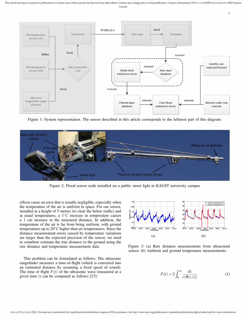
The temperature and distance to the ground measurementsgenerated by the sensor over 6 days (under normal conditions,so that fluctuations are only due to temperature change) areshown in Figure 3. As can be seen from this figure, theraw distance measurements vary significantly over the period(about 12 cm) despite the fact that no flooding occurred overthis period. These variations in observed distance are caused bythe dependency of the speed of sound on air temperature. Formost distance measurement applications, the air temperature



3

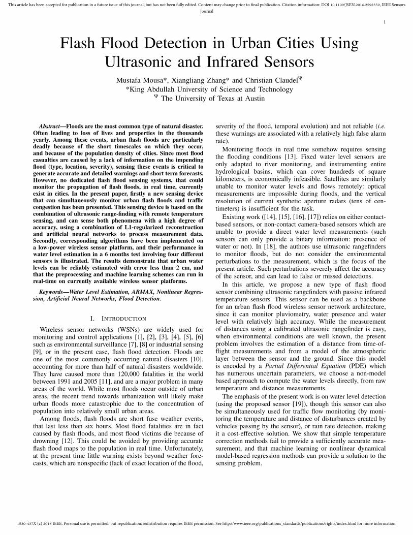
Figure 1: System representation. The sensor described in this article corresponds to the leftmost part of this diagram.

Figure 2: Flood sensor node installed on a public street light in KAUST university campus

effects cause an error that is usually negligible, especially whenthe temperature of the air is uniform in space. For our sensor,installed at a height of 5 meters (to clear the below traffic) andat usual temperatures, a 1◦C increase in temperature causesa 1 cm increase in the measured distance. In addition, thetemperature of the air is far from being uniform, with groundtemperatures up to 20◦C higher than air temperatures. Since thedistance measurement errors caused by temperature variationsare larger than the expected precision of the sensor, we needto somehow estimate the true distance to the ground using theraw distance and temperature measurement data.

This problem can be formulated as follows. The ultrasonicrangefinder measures a time-of-flight (which is converted intoan estimated distance by assuming a fixed speed of sound).The time of flight F(t) of the ultrasonic wave (measured at agiven time t) can be computed as follows [27]:

21/12 22/12 23/12 24/12 25/12 26/12 27/125.25

5.3

5.35

5.4

5.45

5.5

Dis

tan

ce (

m)

Time(Days)

(a)

21/12 22/12 23/12 24/12 25/12 26/12 27/120

10

20

30

40

50

60

Time(Days)

Ambient Temperature(°C)

Ground Temperature(°C)

(b)

Figure 3: (a) Raw distance measurements from ultrasoundsensor. (b) Ambient and ground temperature measurements.

F(t) = 2∫ z0

0

dzc(θ(z, t))

(1)



4

where θ(z) is the air temperature at altitude z. One of themain difficulties arising in this problem is the estimation ofthe function θ(z, t). This function depends on multiple factorsthat are not directly measured by the sensor, including forexample cloud coverage, presence of shadow from buildings,heat island effects and ground albedo. To increase the accuracyof the sensor, we need to estimate the correction to applyto the raw distance measurements of the ultrasonic sensor.The correction factor represents all the perturbations causedby the uneven temperature profile in the air layer below it.For the reasons mentioned above, it is infeasible in practiceto model the air layer temperature using a PDE, since theboundary conditions and the model parameters of the problemare unknown. We thus investigate several model and non-model based approaches to correct the measurements, rangingfrom linear ARMAX models to ANNs.

In this context, our problem is formalized as follows. Letus denote, by e(t), the difference between the measured (i.e.the raw output of the ultrasonic rangefinder) and the actualground distance, which is known when no flash flood occurs.Our objective is to estimate e(t) given Ta(·) and Tg(·), whereTa(·) and Tg(·) are the sensor measurements of the ambientand ground temperatures respectively.

A. Naive temperature correctionWe first investigate the need for a complex temperature com-

pensation model [28] by checking if simpler naive correctionmethods can apply. We know that the measured time of flightis given by equation 1, in which θ(z, t) is unknown. Let usfirst assume that θ(·, t) is constant, that is, the temperature inthe air column is uniform. With this assumption, equation 1,becomes:

F(t) = 2L

c(θ(t))(2)

where θ(t) is the uniform temperature in the air column. Forthe two applications below, we used c(θ(t)) = 331.3+ 0.6 ·θ(t) in m/s, which represents the approximate speed of soundin function of the air temperature θ(t) in ◦C, on a narrowtemperature range around 20◦C.

In Figure 4, we assume that θ(t) = Ta(t), i.e., the air tem-perature in the column is identical to the ambient temperaturemeasured by the infrared sensor. This assumes that the heatingeffects of the sun on the sensors are negligible (that is, thesensor is in thermal equilibrium with the ambient air). Thisoccurs in practice when the wind is very high (which increasesthe heat transfer between the sensor and the air), or when thesolar forcing is negligible (for instance during the night, orduring overcast conditions).

As can be seen from Figure 4, the estimation during thenight is very good, though the compensation fails duringthe day. This is caused both by the assumption that the airtemperature is uniform (which is wrong during the day), and bythe fact that the ambient temperature measured by the sensorcan be higher than the air temperature due to solar forcing.To remove the solar forcing effect on the ambient temperaturemeasurement of the PIR sensor, we used calibrated air tem-perature measurements from the closest weather station. The

21/12 22/12 23/12 24/12 25/12 26/12 27/125.25

5.3

5.35

5.4

5.45

5.5

Time(Days)

Dis

tan

ce (

m)

Raw data from ultrasound

Compensated distance

(a)

15/1 16/1 17/1 18/1 19/1 20/15.25

5.3

5.35

5.4

5.45

5.5

Time(Days)

Dis

tan

ce (

m)

Raw data from ultrasound

Compensated distance

(b)

Figure 4: (a) Predicted distance measurement computed usingambient temperature sensor measurements, and (b) weatherstation air temperature measurements.

corresponding predicted distance measurements are illustratedin Figure 4, and similarly show large variations with time,whereas the actual distance between the sensor and the groundis constant. This shows that the air temperature cannot beassumed to be uniform.

Another simple correction method could be to use theaverage speed of sound in the air layer, assuming that the airtemperature profile θ(z, t) varies linearly between the groundand the sensor, that is:

θ(z, t) = Tg(t)+Ta(t)−Tg(t)

Lz

where L is the distance between the sensor and the ground, andz is the altitude above the ground level. This method does notimprove the accuracy of water level estimate beyond the naivecorrection methods introduced earlier. This analysis shows thatmore advanced methods are needed to estimate the distancebetween the sensor and the ground accurately.

These methods have to rely not only on current tempera-ture measurements, but also on the history of measurements,resulting in a dynamical system. In this article, we investigatevarious models to compensate the thermal effects and correctdistance measurements generated by the sensor. One of thesimplest of such models involves a linear dynamical systemwith inputs, otherwise known as ARMAX (Auto RegressiveMoving Average with Exogenous inputs) models, which wenow investigate.

B. Auto-regressive moving average exogenous (ARMAX) fit-ting

ARMAX can be used for modeling time series and predict-ing future observations by combining a number of previous ob-servations (Autoregressive), a number of noise terms (moving-average), and a number of external (exogenous) inputs, whichare Ta(·) and Tg(·) in the present case. Formally, the error e(t)between the measured distance and the actual distance is givenby:

e(t) =q

∑i=1

ϕie(t− i)+q

∑i=1

θiε(t− i)+

q

∑i=1

ηiTa(t− i)+q

∑i=1

ξiTg(t− i)+ ε(t)(3)



5

where ε(t) is the white noise, ϕi, θi, ηi and ξi are themodel parameters. q is the number of terms considered inautoregressive, in moving-average and in exogenous inputs,or the order of ARMAX model. In our study, we set the orderto a limited number of coefficients (20) in order to avoid over-fitting, and to allow better comparison with other methods.

C. Supervised learningSupervised learning has been extensively studied in machine

learning and has been successfully applied to a wide rangeof applications. Given the inputs and outputs of a system,supervised learning algorithms model the functional relation-ship between inputs and outputs, with no need of knowing thesystem working principles. In other words, it can predict howthe system reacts on the given inputs without knowing howa system works. In our study, the effects of the two temper-ature measurements provided by the sensors on the measureddistance are too difficult to model accurately. Nevertheless,this complex relationship can be modeled through supervisedlearning, with inputs of the ambient and ground temperaturesand outputs of the observed raw distance measurements fromultrasound sensors and the actual distance. Note that whenfloods do not occur (i.e. most of the time), the actual distanceis perfectly known, and the output of the system is the rawdistance measurement generated by the ultrasonic rangefinder.Once the relationship is learned, the actual distance betweenthe sensor and the ground can always be estimated giventhe ambient and ground temperature measurements. Therefore,supervised learning can be viewed as a natural solution to ourwater level prediction problem.

1) Non-Linear regression: The first supervised learningmethod we used is non-linear regression, which models thetarget signal by a non-linear function. In this paper, thefollowing quadratic function is utilized:

e(t) = ∑i(b3i+1Ta(t− k · i)−b3i+2Tg(t− k · i)+b3i+3)

2

where e(t) represents, as before, the difference between mea-sured distance and actual distance at time t. Ta(·) and Tg(·)represent the ambient (sensor) and ground temperatures respec-tively, and b· are the parameters of the non-linear regressionfunction. The combination (k · i) represents the discrete timehorizon used for the prediction. To avoid over-fitting, we chosek = 5, which results in a 15-parameter model taking intoaccount the five most recent pieces of data. This number ofparameters used in this model (15) is comparable to the 20parameters used in the ARMAX analysis detailed above.

This quadratic regression function is selected after em-pirical comparison of models with different parameters. Itis the best performing model that least suffers the over-fitting problem and is more accurate on prediction. Also, theproposed model allows us to capture the influence of the twomeasured temperatures (ambient and ground temperatures) aswell as the coupling (caused by the effects of solar irradiance,the heat island effect and the presence of shadows on theground) between them. The fitting is done through successiveapproximations, for which we limit the number of iterations

to 100 and the tolerance to 10−8. Robust fitting options canbe added to improve the root mean square error performanceof the predicted values.

2) Neural networks: Artificial Neural Networks (ANN) area computational model inspired by the central nervous systemsof animals [29]. This concept and a few possible applicationsin industrial electronics are summarized in [30], [31]. In thisspecific field, there already exist a large number of applicationsof neural networks, some of which include motor drives [32] orpower distribution problems dealing with harmonic distortion.Due to their nonlinear nature, they have also become anintegral part of the field of control systems engineering [33],[34].

a) Neural network architecture: Neural networks can beconsidered as a combination of a set of nonlinear functionsthat are organized structurally layer by layer. They are thusalso called MLPs (Multilayer perceptron). They are well suitedto various application problems due to their “universal approx-imation” property: any continuous function can be uniformlyapproximated to an arbitrary accuracy by neural networks,given enough hidden units with any of a wide variety ofcontinuous nonlinear hidden-layer activation functions, see forinstance [35], [36], and [37].

In our problem setting, there are two inputs (ambient andground temperatures), and one output (the raw distance mea-surement from the ultrasound). Each neuron in the hiddenlayer connecting to the inputs is fed with the input variablesx1, ...,xD. The complete network function is obtained by:

yk(x,w) = α(M

∑j=1

w(2)k j h(

D

∑i=1

w(1)ji xi +b(1)j0 )+b(2)k0 ) (4)

where j = 1, ...,M (M is the total number of hidden neurons inthe this layer). The parameters w(1)

ji and b(1)j0 ( w(2)k j and b(2)k0 ) are

the weights and the biases for the inputs to the first (second)hidden layer. h(.) is an activation function (in the present casethe activation functions are sigmoid functions). The output isa function α(.) (which will be discussed in section III-C2b) ofthe second layer variables. Thus the neural network model canbe considered as a nonlinear function mapping a set of inputvariables {xi} to a set of output variables {yk} controlled bya vector w of adjustable parameters.

b) Levenberg-Marquardt back-propagation training func-tion: Training a neural network involves the tuning of theweights and biases of the network. The objective is to maxi-mize the network prediction performance, which correspondsto minimizing the difference between all network outputsyk and desired outputs or targets tk on validation data. Thecomputational time required for the training algorithm dependson many factors, including the complexity and objective func-tion of the problem, the size of training data, the number ofparameters in the network, and whether the network is beingused for pattern recognition (discriminant analysis) or functionapproximation (regression [36]). For our particular problem,we are interested in the function approximation problem witha few hundred weights in a moderate size network. In thisspecific case, the Levenberg-Marquardt algorithm has beenproven to have the fastest convergence [38]. It updates the



6

network weights and biases in the direction in which theperformance function decreases most rapidly. This advantageis more noticeable when implementing NN on the proposedplatform of this work, since sensors have a limited bandwidth,and that transmitting all the data would be energy intensive,thus it is very critical to consider efficient online training.

Having stated all of this and tried different modules. Werealized that we need an efficient preprocessing tool in additionto the online training. Indeed, the raw data generated by the in-frared temperature sensors and the ultrasound rangefinder havedifferent scales, and sometimes exhibiting inconsistencies, ascan be observed in Figure 3 which is a major game changerin our application. Therefore, an effective preprocessing pro-cedure is essential in the accurate sensing of floods based onmeasurement data produced from sensor nodes.

IV. PROPOSED SOLUTION AND SYSTEM PERFORMANCE

A. Preprocessing of measurement data

As stated previously in section III, the raw data generated bythe infrared temperature sensors and the ultrasound rangefinderhave different scales, and are sometimes exhibiting inconsis-tencies. We propose a preprocessing procedure as illustrated inFigure 5. It mainly involves two main processes: fault detectionand missing data reconstruction.

1) Sensor fault detection: Sensor faults can be caused bymultiple factors. In the present case, these faults were mainlydue to gateway failures (due to a loss of the internet connec-tion), and brownouts of the sensor caused by faulty chargingcircuits in a narrow solar power input range when collectingthe measurement data.

We first check the network faults (communication faults),which are identified by detecting time periods that have morethan 15 minutes (i.e. 90 samples at the 0.1Hz message updaterate) without reception of data from sensors. When suchfaults are detected, the missing data in the blank periodsare reconstructed directly by the LASSO-based formulation(least absolute shrinkage and selection operator) which will beexplain in the following section. To remove outliers (caused byvehicles passing below the sensor), we apply a moving medianfilter to the temperature and distance data. Finally, we detectsensor fault by analyzing the consensus among all six infraredtemperature sensors in the node. Whereas for the ambienttemperature and the distance measurements the consensus isnot applicable since we have one of each in a sensor node. Wethen use a sliding window, in which we calculate the mean µand the standard deviation σ of the measurement data of allthe sensors . The records that deviate more than 3σ from themean are considered anomalies, and excluded from the dataset.Since the main cause of sensor noise is thermal noise [39], thesensor measurements follow a normal distribution, given thatthe thermal anomalies caused by the vehicles are suppressedby the median filter. Hence, 99.7% of the values fall withinthe [µ−3σ,µ+3σ] window. Most of the data excluded usingthis approach is indeed faulty data. All data gone through thefault detection process are stored and served to the next step,approximating the missing data to complete the measurements.

2) L1 regularized reconstruction: In order to reconstructthe missing data in real-time, we leverage the data generatedduring the previous days as follows. Let us consider the timeseries si(·), obtained during the previous i ∈ {0, ..., imax} days,and let j ∈ {0, ..., jmax} represent a time index in a day (inpractice, j ranges from 0 to 8640 since we have a sampling rateof 0.1Hz). We assume that the current measurements s( j) canbe written as a linear combination of the past measurements,as follows:

sestimate( j) =imax

∑i=0

αisi( j) (5)

where α1, · · · ,αimax are model parameters. Finding these pa-rameters can be done by minimizing the estimation error, forexample in the least squares sense:

minα

∑j∈J

(imax

∑i=1

αisi( j)− s0( j)

)2

(6)

where J ⊂ {0, ..., jmax} is the set of times (for the current day)associated with non-faulty measurements. s0 is the current daymeasurements.

In general, |J| is considerably larger than imax, and the prob-lem is overdetermined. The main issue with this formulation isthe fact that any given day should only have a few identifiablefeatures from the previous days patterns, and thus, α shouldbe sparse. To enforce this sparsity constraints, we add a L1norm regularization term to the above formulation, leading tothe formulation of our estimation problem as a LASSO [40]:

minα

∑j∈J

(imax

∑i=1

αisi( j)− s0( j)

)2

+λ||α||1 (7)

where λ is the regularization parameter that trades off fittingquality and sparsity. Sparsity also improves the robustness ofthe regression to noise.

Problem (7) is a quadratic program (QP) which can besolved using standard convex optimization methods. The re-sults of the preprocessing scheme is illustrated in Figure 6. Inthis Figure, we show the raw measurement data, along withthe output of the fault detection stage, and the output of theLASSO-based data reconstruction stage. We applied the abovealgorithms to filter measurement data over extended periods oftime. Figure 7 illustrates the reconstructed measurement databetween December 4th 2013 and December 21st 2013, whichis used as training data for the artificial neural network-basedwater level estimation scheme, introduced in the subsequentsections.

This section reports the performance of different modelswe studied in the previous section. The data set used in thisvalidation has been generated from the sensors deployed onour university’s campus.

B. Artificial neural networks performanceThe number of neurons has been set to achieve good

performance on the validation dataset, considering the trade offbetween the computational time required to train the network



7

Sensor node measurements(Input) No

Yes

moving median filter

To water level estimation models (output)








Comm. fault detection (absence of samples within a time period)

Sensor fault detection (local time consensus

thresholding)

Sensor fault detection (local time thresholding)

Tground1

Tground2

Tground6

Tground3

Tground4

Tground5

Tair

distance

Delete corresponding

data

Faulty dataFaulty data

Non faulty data (Tground5)

Non faulty data

Data repositoryLASSO-based formulation

LASSO parameters estimation

NormalizationCleaned dataL1 regularized

reconstruction

LASSO parameters

Figure 5: The preprocessing of the measured data from the sensor node. The processed data are served to the estimation models.

Time(Days)

7/12 8/12 9/12 10/12 11/12 12/12 13/12 14/12 15/12

Tem

pera

ture

(°C

)

0

10

20

30

40

50

60Raw data from PIR sensors Output of fault detection methodPredicted data (LASSO)

Figure 6: Comparison between raw PIR sensor data (blue) andreconstructed PIR data (green) at the end of the preprocessingstage for a sample of the data in December (without normal-ization).

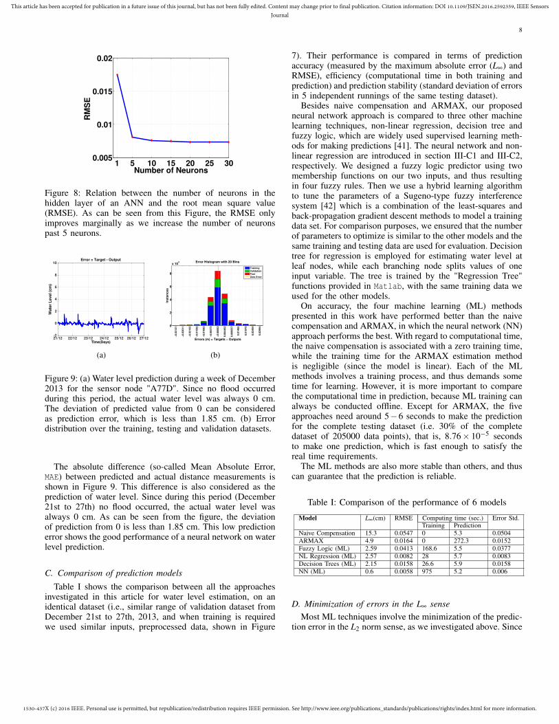
and the performance of root mean square error (RMSE) thatcan be reached. Furthermore, we had to fix the number ofneurons to be comparable with the other methods we used toestimate the water level (since the number of neurons deter-mines the number of coefficients to be optimized). RMSE onlyimproves marginally as we increase the number of neurons past5 neurons, as can be seen from Figure 8.

We implemented the neural network model using the neuralnetwork toolbox of Matlab, running on a Mackbook i7. Wewere able to evaluate and train the neural network using theLevenberg-Marquardt algorithm with one hidden layer of 10neurons in a two inputs and one output setting.

The dataset consists of 205000 data points, as illustrated in

4/12 5/12 6/12 7/12 8/12 9/12 10/12 11/12 12/12 13/12 14/12 15/12 16/12 17/12 18/12 19/12 20/12 21/12

−2

−1

0

1

2

3Normalized Targets

Time(Days)

4/12 5/12 6/12 7/12 8/12 9/12 10/12 11/12 12/12 13/12 14/12 15/12 16/12 17/12 18/12 19/12 20/12 21/12−2

0

2

4Normalized Inputs

Time(Days)

Ground Temperature

Ambient Temperature

Raw Data from ultrasound

Figure 7: Top: Normalized and filtered raw distance mea-surements (for the preprocessed training dataset). Bottom:Normalized and filtered ambient and ground temperature mea-surements (for the preprocessed training dataset).

Figure 7. We arbitrarily divided it into a training dataset, avalidation dataset and a testing dataset. The training datasetcorresponds to 70% of the overall data, while the validationand testing datasets correspond to 15% of the data each.The validation dataset is used during the training process, tohalt training when the performance of the estimation on thevalidation dataset stops improving.

Figure 9 shows the histogram of the error between outputand targets for the training, validation and testing samples.It can be seen in the figure that the histogram fits a normaldistribution with a maximum detected error on validation andon testing samples of less than 2 cm.



8

1 5 10 15 20 25 300.005

0.01

0.015

0.02

Number of Neurons

RM

SE

Figure 8: Relation between the number of neurons in thehidden layer of an ANN and the root mean square value(RMSE). As can be seen from this Figure, the RMSE onlyimproves marginally as we increase the number of neuronspast 5 neurons.

Time(Days)21/12 22/12 23/12 24/12 25/12 26/12 27/12

Wa

ter

Le

ve

l (c

m)

-2

0

2

4

6

8

10Error = Target - Output

(a)

0

2

4

6

8

x 104 Error Histogram with 20 Bins

Ins

tan

ce

s

Errors (m) = Targets − Outputs

−0.0

3121

−0.0

2611

−0.0

2102

−0.0

1592

−0.0

1082

−0.0

0573

−0.0

0063

0.0

04462

0.0

09557

0.0

1465

0.0

1975

0.0

2484

0.0

2994

Training

Validation

Test

Zero Error

(b)

Figure 9: (a) Water level prediction during a week of December2013 for the sensor node "A77D". Since no flood occurredduring this period, the actual water level was always 0 cm.The deviation of predicted value from 0 can be consideredas prediction error, which is less than 1.85 cm. (b) Errordistribution over the training, testing and validation datasets.

The absolute difference (so-called Mean Absolute Error,MAE) between predicted and actual distance measurements isshown in Figure 9. This difference is also considered as theprediction of water level. Since during this period (December21st to 27th) no flood occurred, the actual water level wasalways 0 cm. As can be seen from the figure, the deviationof prediction from 0 is less than 1.85 cm. This low predictionerror shows the good performance of a neural network on waterlevel prediction.

C. Comparison of prediction models

Table I shows the comparison between all the approachesinvestigated in this article for water level estimation, on anidentical dataset (i.e., similar range of validation dataset fromDecember 21st to 27th, 2013, and when training is requiredwe used similar inputs, preprocessed data, shown in Figure

7). Their performance is compared in terms of predictionaccuracy (measured by the maximum absolute error (L∞) andRMSE), efficiency (computational time in both training andprediction) and prediction stability (standard deviation of errorsin 5 independent runnings of the same testing dataset).

Besides naive compensation and ARMAX, our proposedneural network approach is compared to three other machinelearning techniques, non-linear regression, decision tree andfuzzy logic, which are widely used supervised learning meth-ods for making predictions [41]. The neural network and non-linear regression are introduced in section III-C1 and III-C2,respectively. We designed a fuzzy logic predictor using twomembership functions on our two inputs, and thus resultingin four fuzzy rules. Then we use a hybrid learning algorithmto tune the parameters of a Sugeno-type fuzzy interferencesystem [42] which is a combination of the least-squares andback-propagation gradient descent methods to model a trainingdata set. For comparison purposes, we ensured that the numberof parameters to optimize is similar to the other models and thesame training and testing data are used for evaluation. Decisiontree for regression is employed for estimating water level atleaf nodes, while each branching node splits values of oneinput variable. The tree is trained by the "Regression Tree"functions provided in Matlab, with the same training data weused for the other models.

On accuracy, the four machine learning (ML) methodspresented in this work have performed better than the naivecompensation and ARMAX, in which the neural network (NN)approach performs the best. With regard to computational time,the naive compensation is associated with a zero training time,while the training time for the ARMAX estimation methodis negligible (since the model is linear). Each of the MLmethods involves a training process, and thus demands sometime for learning. However, it is more important to comparethe computational time in prediction, because ML training canalways be conducted offline. Except for ARMAX, the fiveapproaches need around 5−6 seconds to make the predictionfor the complete testing dataset (i.e. 30% of the completedataset of 205000 data points), that is, 8.76× 10−5 secondsto make one prediction, which is fast enough to satisfy thereal time requirements.

The ML methods are also more stable than others, and thuscan guarantee that the prediction is reliable.

Table I: Comparison of the performance of 6 models

Model L∞(cm) RMSE Computing time (sec.) Error Std.Training Prediction

Naive Compensation 15.3 0.0547 0 5.3 0.0504ARMAX 4.9 0.0164 0 272.3 0.0152Fuzzy Logic (ML) 2.59 0.0413 168.6 5.5 0.0377NL Regression (ML) 2.57 0.0082 28 5.7 0.0083Decision Trees (ML) 2.15 0.0158 26.6 5.9 0.0158NN (ML) 0.6 0.0058 975 5.2 0.006

D. Minimization of errors in the L∞ senseMost ML techniques involve the minimization of the predic-

tion error in the L2 norm sense, as we investigated above. Since



9

flash floods are extremely rare events, we are also interestedin making prediction with minimized error in the L∞ sense, toavoid false alarms in the flood monitoring system. The infinitynorm is better than norm 2 for the task, since we want to detectevents based on thresholding, and a very low norm 2 (but highnorm infinity) in the training (non flood) data is unacceptable,since it would lead to false detections.

Our objective in this subsection is thus, technically tominimize the prediction error in the L∞ sense instead of the L2norm sense, though the L∞ error usually improves when theL2 error is reduced.

Minimizing the prediction error in the L∞ sense is straight-forward in the case of a linear model: it can be formally writtenas:

minW‖XW −Y‖∞

where X is the input, W is the model coefficient to beoptimized, and Y is the output. This resulting Linear Program(LP) problem is solved by the SDPT3 package working underMatlab in this paper.

We investigate both the linear model (ARMAX) and thenonlinear model (non-linear regression) for minimizing errorin L∞. Table II shows the performance of ARMAX and non-linear regression, measured in maximum absolute difference(L∞), RMSE and standard deviation of errors (in 5 independentrunnings of the same testing dataset). Comparing the L∞ valuesof these two methods in Table II and Table I, we can see thatthey have smaller L∞ when minimizing L∞ error than whenminimizing L2 error. The non-linear regression model withminimized L∞ error is comparable to the ANN model withminimized L2 error, which is the best as observed in Table I.

With regard to the RMSE, both ARMAX and non-linearregression have high error value when minimizing error in L∞.This is understandable, as, by nature, they lead to small RMSE(a performance metric defined in L2) when minimizing errorin L2.

Table II: Comparison between ARMAX and NL regressionwhen minimizing error in L∞

Model L∞(cm) RMSE Error Std.ARMAX 2.28 1.2593 1.0128NL Regression (ML) 0.55 0.3218 0.2572

E. Temporal robustness of ANN model parametersIn this section, we evaluate the time dependence of the

training parameters. For this, we train the artificial neuralnetwork model using data from the early December (December4th to 21st), and validate the performance on three differentsets of data (temporally separated), namely late December(December 21st to 27th), January and February.

Table III shows the performance of the estimation models ofthe neural networks on the sensor node "A77D" using trainingdata from early December 2013 only. As can be noted, theprediction performance slightly degrades in February. How-ever, the estimation error is acceptable (within about 2 cm)

for flash flood monitoring applications. This suggests that thecoefficient can be used for large durations (e.g., tens of days)before degrading (hence it needs to be tuned), which enableslarge datasets to be integrated in the training process.

Table III: Evaluation of temporal robustness: comparing pre-diction accuracy in different months when using NN trainedby data in early December, 2013.

Month L∞(cm) RMSE Error Std.Late December 1.63 0.0215 0.0213January 2.08 0.0267 0.0267February 2.15 0.0272 0.0272

F. Spatial robustness analysis of ANN modelTo evaluate the robustness of the model parameters with

respect to spatial changes, we installed two sensor nodes ina close proximity (during January 2014): sensors "A77D" and"8F90". Node "8F90" is placed in an area that can be shadowedby a building at some times of the day, unlike node "A77D".

In a similar manner to the analysis done to "A77D", weestimated the water level and the norm infinity error ofestimation during a period of 11 days is shown in Figure 10(picked right after we installed the node early in January 2014).It can be seen from Figure 10 that the error is less than 0.6cm.

Then, in order to evaluate the spatial robustness, the neuralnetwork is trained by data from sensor "A77D" during De-cember 4th and 21st, 2013, to predict the data for the sensornode "8F90" over the same testing period of the 11 days.

As expected, the performance of the prediction of "8F90"slightly degrades in this case: RMS error of 0.275 vs. 0.0058and norm infinity error of 1.735 cm vs. 0.6 cm for the trainingwith the data of "8F90", compared to the training with the dataof "A77D". This acceptable error (i.e. less than 2 cm) allowsus in practice to use training data from the nearest sensors toimmediately generate distance measurement data from a newlyinstalled sensor, without having to wait for a training period.

G. Validation on an actual flooding incidentFlood incidents are usually rare, but one such incidents

occurred in the test period, the only incident which hasoccurred to date. This incident has been detected by twosensors installed in Umm Al Qura University in Mecca, SaudiArabia, where climate conditions differ and floods are morefrequent. The flash flood occurred on the 8th of May 2014,and, fortunately, did not result in extreme damage and causedonly a single casualty [43]. Students at the university reportedthat the street water level was locally around 10cm, and theincident started at around 11PM local time.

This incident has been captured by the two sensors "8F48"and "D3CB". The water level estimates (using the days beforeMay 6th as training data for both sensors) are illustrated inFigure 11 for both sensors. As can be seen from this Figure,the flood is clearly detected, and corresponds to a significant



10

28/1 7/2−2

012

4

6

8

10

11 Days (from Januray 28th till February the 7th)

Wate

r L

evel (c

m)

Sensor Node "8F90"

Figure 10: Estimated water level at the sensor node "8F90"from January 28 to February 7, 2014. In this test, the artificialneural network is trained onboard by the sensor node itself.

rise in the water level estimate. We can also see the onset ofthe flood is identical for both sensors, and that the estimatedwater levels are of the same order of magnitude (7 to 9 cm).

Unfortunately, the sink node has failed shortly after theflood occurred, around 11:30 PM. The failure of the sink nodewas probably caused by an electrical failure related to theflooding event. Nevertheless, the available data clearly showsthe detection of a minor event shortly before midnight, 9th ofMay 2014, on both sensors. There was no way to detect the

6/5 7/5 8/5 9/5

−2

0

2

4

6

8

10

Time (Days)

Wa

ter

Le

ve

l (c

m)

Sensor Node "DC3B"

Flood detection

6/5 7/5 8/5 9/5

−2

0

2

4

6

8

10

Time (Days)

Wa

ter

Le

ve

l (c

m)

Sensor Node "8F48"

Flood detection

Figure 11: Water level estimation between May 6 and May 9,2014, for sensor nodes "DC3B" and "8F48" deployed in UmmAl Qura University campus.

flood incident from the raw data of the ultrasonic, as illustratedin Figure 12 for one of the sensor nodes that encountered theflood (i.e. "8F48"). As shown by this Figure, naive thresholdingon the raw water level measurement data would not allow oneto detect the flood.

V. IMPLEMENTATION OF ANN ALGORITHMS ONMICROCONTROLLERS

In order to validate our design and be able in practiceto use our solution, we implement our algorithms on thededicated microcontroller board and validate the performanceas explained in the following sections.

6/5 7/5 8/5 9/5Time(Days)

510

515

520

525

530

535

Measu

red

dis

tan

ce (

cm

)

Sensor Node "DC3B"

6/5 7/5 8/5 9/5Time(Days)

510

515

520

525

530

535

Measu

red

dis

tan

ce (

cm

)

Sensor Node "8F48"

Figure 12: Raw ultrasonic measurements between May 6 andMay 9, 2014, for sensor nodes "DC3B" and "8F48" deployedin Umm Al Qura University campus.

A. Dedicated sensing platform for flash flood monitoring ap-plications

In the present case, we have built a customized hard-ware platform, described in the companion article [26]. Thisplatform is built around a 32-bit microcontroller and illus-trated in Figure 13. We selected for this application, theSTM32F407, a 32-bit ARM Cortex-M4 based microcontrollerfrom ST Microelectronics since it satisfies the requirementsof our estimation problem and best trades off RAM, powerconsumption, cost and most importantly for this study, com-putation (since this sensor is sensing traffic flow, relayingand forwarding other messages in the sensor network, andestimating traffic flow conditions [25]).

Figure 13: Custom-developed 32-bit microcontroller platform(9cm x 6.5cm) connected to an XBee module and to PIR andultrasonic sensors.

B. On-Board Neural Network Algorithm

In order to build a neural network on the custom-basedmicrocontrollers, we need to build not only the architecture butalso the data storage system, for performing both training andprediction. The key values to be stored are weights associated



11

with neurons, the weight updates and error gradients duringthe training phase.

1) Initialization of the Neural Network: To minimize thenumber of iterations in neural network training before conver-gence, the weights associated with neurons should be carefullyinitialized. Since our simulation results from training data setalready show good estimation performance, and good spatio-temporal robustness, as shown in sections IV-E and IV-F, theweights of the trained neural network of any given sensor is agood initial guess. Therefore, we initialize the neural networkon board by the weights of the neural network trained inthe simulation from training data between December 4th tillDecember 21st.

2) Neural Network Training: As we have illustrated pre-viously in section IV-E, and in Figure 14, the trained NNmodel is robust when it is applied to long term predictionover two months until the error propagates due to the weatherchange. In order to continuously make accurate prediction, theNN model should be updated with the recently received data,which are saved in a 2GB micro SD card. The card has thecapacity to host at most 12 months of data, which are sufficientfor NN updating. Due to the limited computing power on

1 week (late December) 1 week (January) 1 week (February)

-2

0

2

4

6

8

10

Wa

ter

Le

ve

l (c

m)

Figure 14: Prediction accuracy during different months on thesensor node "A77D" installed on our campus in November2013, using training data from December 2013 only. As canbe seen from this Figure, the prediction performance slightlydegrades in February, though its performance is still acceptablefor flash flood monitoring applications.

board, updating the NN cannot be implemented in the batchmode introduced in section III-C2b. The main reason is therepeatedly heavy computation of yk in Equation 4 for all xin training data during the error propagation process. Thus weadopt the online training mode for updating the weights in NNmodel, due to its comparable performance to the batch modebut better efficiency. Instead of taking all x in training data fora single update of weights in NN, the online mode updatesthe weights by using x one by one. That is to say, the datasaved in SD card flow into the NN individually and update ituntil the prediction error is reduced down below an acceptablethreshold (e.g., 2 cm in the L∞ case).

3) Implementation: The implementation of code is doneusing Keil v4.7 [44] which is a software provided by theARM group, and optimized for C/C++ language. We have

implemented our algorithms on the wireless sensor nodesusing a conventional back-propagation neural network classin C language that makes use of gradient descent, withparameters defined as: 0.001 learning late, 1500 of maxi-mum epochs during training, and maximum accuracy. Thedemonstration code is a 996 lines written in C++ languageand is built on top of <math.h>, <algorithm>, <fstream>,<string>, <vector>, <stdio.h> libraries, as well as thedesigned neural network class "neuralnetwork.h". The codecan toggle between batch and online training mode, and getsthe training stopping criteria from the user. Its total memorysize (when compiled) is 101 kB (our microcontroller’s ROMsize is 1 MB), while its peak memory usage is 58 kB (ourmicrocontroller total RAM size is 192 kB), well below thelimits of the Cortex M4 microcontroller.

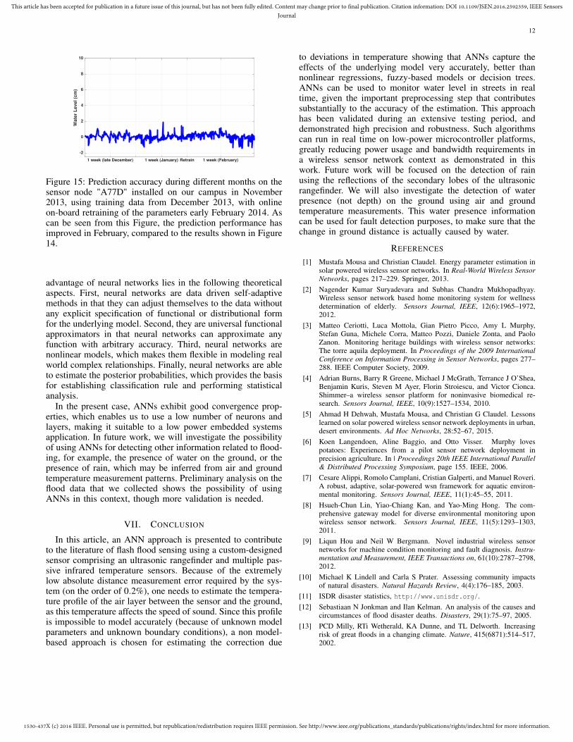
4) Neural Network performance: We coded the neural net-work algorithm on the custom-based microcontroller platformdescribed earlier, and tested them for real time performance.The prediction performance of the NN running on the compu-tational platforms has similar results to the ones obtained onMatlab. However, since the platform has less computationalcapabilities than a computer, its computational time was ex-pected to be much greater when we consider the training inaddition to the prediction of the data in order to converge tothe solution. We show the performance on the prediction ofwater level with retraining when the threshold is exceeded atthe beginning of February 2014 in Figure 15. We used oneweek of data following the online training approach to retrainthe NN parameters and as we can see this helped bringing theerror to within 2 cm. The computational time measured forthe process of training and predicting a week of data onboardwith the online training approach took approximately, 118minutes (11.2 minutes for prediction). We implement the on-board NN on the custom-based microcontroller platform, andevaluate its performance to see whether prediction error canbe reduced after online updating. In Figure 14, we show theperformance on the prediction of water level with training datafrom December 2013 only. It can be seen that the predictionperformance slightly degrades in February 2014 (sometimeswith errors greater than 2 cm). In Figure 15, we show theprediction with online training when the error exceeded 2 cmat the beginning of February 2014. We used one week ofdata following the online training mode to update the NNparameters. We can see that the error is reduced to be lessthan 2 cm.

Due to the limited computational capability of the low-power platform, the online training mode took about 2 hoursfor absorbing the one week data, while the prediction isquite fast 0.03 seconds per data sample. Therefore, the onlinetraining employed only one week data and stopped to proceedwith more data to further reduce the error that is already lessthan 2 cm.

VI. DISCUSSION

The recent vast research activities in neural classificationhave established that neural networks are a promising al-ternative to various conventional classification methods. The



12

1 week (late December) 1 week (January) Retrain 1 week (February)

-2

0

2

4

6

8

10

Wa

ter

Le

ve

l (c

m)

Figure 15: Prediction accuracy during different months on thesensor node "A77D" installed on our campus in November2013, using training data from December 2013, with onlineon-board retraining of the parameters early February 2014. Ascan be seen from this Figure, the prediction performance hasimproved in February, compared to the results shown in Figure14.

advantage of neural networks lies in the following theoreticalaspects. First, neural networks are data driven self-adaptivemethods in that they can adjust themselves to the data withoutany explicit specification of functional or distributional formfor the underlying model. Second, they are universal functionalapproximators in that neural networks can approximate anyfunction with arbitrary accuracy. Third, neural networks arenonlinear models, which makes them flexible in modeling realworld complex relationships. Finally, neural networks are ableto estimate the posterior probabilities, which provides the basisfor establishing classification rule and performing statisticalanalysis.

In the present case, ANNs exhibit good convergence prop-erties, which enables us to use a low number of neurons andlayers, making it suitable to a low power embedded systemsapplication. In future work, we will investigate the possibilityof using ANNs for detecting other information related to flood-ing, for example, the presence of water on the ground, or thepresence of rain, which may be inferred from air and groundtemperature measurement patterns. Preliminary analysis on theflood data that we collected shows the possibility of usingANNs in this context, though more validation is needed.

VII. CONCLUSION

In this article, an ANN approach is presented to contributeto the literature of flash flood sensing using a custom-designedsensor comprising an ultrasonic rangefinder and multiple pas-sive infrared temperature sensors. Because of the extremelylow absolute distance measurement error required by the sys-tem (on the order of 0.2%), one needs to estimate the tempera-ture profile of the air layer between the sensor and the ground,as this temperature affects the speed of sound. Since this profileis impossible to model accurately (because of unknown modelparameters and unknown boundary conditions), a non model-based approach is chosen for estimating the correction due

to deviations in temperature showing that ANNs capture theeffects of the underlying model very accurately, better thannonlinear regressions, fuzzy-based models or decision trees.ANNs can be used to monitor water level in streets in realtime, given the important preprocessing step that contributessubstantially to the accuracy of the estimation. This approachhas been validated during an extensive testing period, anddemonstrated high precision and robustness. Such algorithmscan run in real time on low-power microcontroller platforms,greatly reducing power usage and bandwidth requirements ina wireless sensor network context as demonstrated in thiswork. Future work will be focused on the detection of rainusing the reflections of the secondary lobes of the ultrasonicrangefinder. We will also investigate the detection of waterpresence (not depth) on the ground using air and groundtemperature measurements. This water presence informationcan be used for fault detection purposes, to make sure that thechange in ground distance is actually caused by water.

REFERENCES

[1] Mustafa Mousa and Christian Claudel. Energy parameter estimation insolar powered wireless sensor networks. In Real-World Wireless SensorNetworks, pages 217–229. Springer, 2013.

[2] Nagender Kumar Suryadevara and Subhas Chandra Mukhopadhyay.Wireless sensor network based home monitoring system for wellnessdetermination of elderly. Sensors Journal, IEEE, 12(6):1965–1972,2012.

[3] Matteo Ceriotti, Luca Mottola, Gian Pietro Picco, Amy L Murphy,Stefan Guna, Michele Corra, Matteo Pozzi, Daniele Zonta, and PaoloZanon. Monitoring heritage buildings with wireless sensor networks:The torre aquila deployment. In Proceedings of the 2009 InternationalConference on Information Processing in Sensor Networks, pages 277–288. IEEE Computer Society, 2009.

[4] Adrian Burns, Barry R Greene, Michael J McGrath, Terrance J O’Shea,Benjamin Kuris, Steven M Ayer, Florin Stroiescu, and Victor Cionca.Shimmer–a wireless sensor platform for noninvasive biomedical re-search. Sensors Journal, IEEE, 10(9):1527–1534, 2010.

[5] Ahmad H Dehwah, Mustafa Mousa, and Christian G Claudel. Lessonslearned on solar powered wireless sensor network deployments in urban,desert environments. Ad Hoc Networks, 28:52–67, 2015.

[6] Koen Langendoen, Aline Baggio, and Otto Visser. Murphy lovespotatoes: Experiences from a pilot sensor network deployment inprecision agriculture. In | Proceedings 20th IEEE International Parallel& Distributed Processing Symposium, page 155. IEEE, 2006.

[7] Cesare Alippi, Romolo Camplani, Cristian Galperti, and Manuel Roveri.A robust, adaptive, solar-powered wsn framework for aquatic environ-mental monitoring. Sensors Journal, IEEE, 11(1):45–55, 2011.

[8] Hsueh-Chun Lin, Yiao-Chiang Kan, and Yao-Ming Hong. The com-prehensive gateway model for diverse environmental monitoring uponwireless sensor network. Sensors Journal, IEEE, 11(5):1293–1303,2011.

[9] Liqun Hou and Neil W Bergmann. Novel industrial wireless sensornetworks for machine condition monitoring and fault diagnosis. Instru-mentation and Measurement, IEEE Transactions on, 61(10):2787–2798,2012.

[10] Michael K Lindell and Carla S Prater. Assessing community impactsof natural disasters. Natural Hazards Review, 4(4):176–185, 2003.

[11] ISDR disaster statistics, http://www.unisdr.org/.[12] Sebastiaan N Jonkman and Ilan Kelman. An analysis of the causes and

circumstances of flood disaster deaths. Disasters, 29(1):75–97, 2005.[13] PCD Milly, RTi Wetherald, KA Dunne, and TL Delworth. Increasing

risk of great floods in a changing climate. Nature, 415(6871):514–517,2002.



13

[14] M Castillo-Effer, Daniel H Quintela, W Moreno, R Jordan, and W West-hoff. Wireless sensor networks for flash-flood alerting. In Devices,Circuits and Systems, 2004. Proceedings of the Fifth IEEE InternationalCaracas Conference on, volume 1, pages 142–146. IEEE, 2004.

[15] Endrowednes Kuantama, Leonardy Setyawan, and Jessie Darma. Earlyflood alerts using short message service (sms). In System Engineeringand Technology (ICSET), 2012 International Conference on, pages 1–5.IEEE, 2012.

[16] CL Lai, JC Yang, and YH Chen. A real time video processing basedsurveillance system for early fire and flood detection. In Instrumentationand Measurement Technology Conference Proceedings, 2007. IMTC2007. IEEE, pages 1–6. IEEE, 2007.

[17] Hongyan Fu, Xuewen Shu, Aping Zhang, Weisheng Liu, Lin Zhang,Sailing He, and Ian Bennion. Implementation and characterization ofliquid-level sensor based on a long-period fiber grating mach–zehnderinterferometer. Sensors Journal, IEEE, 11(11):2878–2882, 2011.

[18] Ni-Bin Chang and Da-Hai Guo. Urban flash flood monitoring, mappingand forecasting via a tailored sensor network system. In Networking,Sensing and Control, 2006. ICNSC’06. Proceedings of the 2006 IEEEInternational Conference on, pages 757–761. IEEE, 2006.

[19] Mustafa Mousa, Enas Oudat, and Christian Claudel. A novel dualtraffic/flash flood monitoring system using passive infrared/ultrasonicsensors. In Mobile Ad Hoc and Sensor Systems (MASS), 2015 IEEE12th International Conference on, pages 388–397. IEEE, 2015.

[20] Mustafa Mousa and Christian Claudel. Water level estimation in urbanultrasonic/passive infrared flash flood sensor networks using supervisedlearning. In Proceedings of the 13th international symposium onInformation processing in sensor networks (IPSN), pages 277–278.IEEE Press, 2014.

[21] VE Sakharov, SA Kuznetsov, BD Zaitsev, IE Kuznetsova, and SG Joshi.Liquid Level Sensor Using Ultrasonic Lamb Waves. Ultrasonics,41(4):319–322, 2003.

[22] Richard Hunter Brown. Liquid Level Sensor, December 16 1997. USPatent 5,697,248.

[23] Elizabeth A Basha, Sai Ravela, and Daniela Rus. Model-BasedMonitoring for Early Warning Flood Detection. In Proceedings of the6th ACM conference on Embedded network sensor systems, pages 295–308. ACM, 2008.

[24] Chih-Wei Lai, Yu-Lung Lo, Jiahn-Piring Yur, and Chin-Ho Chuang.Application of fiber bragg grating level sensor and fabry-perot pressuresensor to simultaneous measurement of liquid level and specific gravity.Sensors Journal, IEEE, 12(4):827–831, 2012.

[25] Edward Canepa, Enas Odat, Ahmad Dehwah, Mustafa Mousa, JimingJiang, and Christian Claudel. A sensor network architecture for urbantraffic state estimation with mixed Eulerian/Lagrangian sensing based ondistributed computing. 27th Conference on Architecture of ComputingSystems, 2014.

[26] Jiming Jiang and Christian Claudel. A wireless computational platformfor distributed computing based traffic monitoring involving mixedeulerian-lagrangian sensing. In Industrial Embedded Systems (SIES),2013-8th IEEE International Symposium on, pages 232–239. IEEE,2013.

[27] Daniele Marioli, Claudio Narduzzi, Carlo Offelli, Dario Petri, Emilio

Sardini, and Andrea Taroni. Digital time-of-flight measurement forultrasonic sensors. IEEE Transactions on Instrumentation and Mea-surement, 41(1):93–97, 1992.

[28] Jagdish Chandra Patra, Pramod Kumar Meher, and GoutamChakraborty. Development of laguerre neural-network-based intelligentsensors for wireless sensor networks. Instrumentation and Measure-ment, IEEE Transactions on, 60(3):725–734, 2011.

[29] Jagdish Chandra Patra, Alex C Kot, and Ganapati Panda. An intelligentpressure sensor using neural networks. Instrumentation and Measure-ment, IEEE Transactions on, 49(4):829–834, 2000.

[30] Bimal K Bose. Neural network applications in power electronics andmotor drives an introduction and perspective. Industrial Electronics,IEEE Transactions on, 54(1):14–33, 2007.

[31] Magali RG Meireles, Paulo EM Almeida, and Marcelo Godoy Simões.A comprehensive review for industrial applicability of artificial neuralnetworks. Industrial Electronics, IEEE Transactions on, 50(3):585–601,2003.

[32] Franck Betin, Arnaud Sivert, Amine Yazidi, and G-A Capolino. De-termination of scaling factors for fuzzy logic control using the sliding-mode approach: Application to control of a dc machine drive. IndustrialElectronics, IEEE Transactions on, 54(1):296–309, 2007.

[33] Shuzhi Sam Ge and Cong Wang. Adaptive neural control of uncertainmimo nonlinear systems. Neural Networks, IEEE Transactions on,15(3):674–692, 2004.

[34] Frank L Lewis, Aydin Yesildirek, and Kai Liu. Multilayer neural-net robot controller with guaranteed tracking performance. NeuralNetworks, IEEE Transactions on, 7(2):388–399, 1996.

[35] Kurt Hornik, Maxwell Stinchcombe, and Halbert White. Multilayerfeedforward networks are universal approximators. Neural networks,2(5):359–366, 1989.

[36] Christopher M Bishop et al. Pattern recognition and machine learning,volume 1. springer New York, 2006.

[37] Brian D Ripley and Ruth M Ripley. Neural networks as statisticalmethods in survival analysis. Clinical applications of artificial neuralnetworks, pages 237–255, 2001.

[38] Jorge J Moré. The levenberg-marquardt algorithm: implementation andtheory. In Numerical analysis, pages 105–116. Springer, 1978.

[39] Seong Taek Chung, Seung Jean Kim, Jungwon Lee, and John MCioffi. A game-theoretic approach to power allocation in frequency-selective gaussian interference channels. In in Proc. IEEE InternationalSymposium on Inform. Theory, Pacifico. Citeseer, 2003.

[40] Mark Schmidt. Least squares optimization with l1-norm regularization.CS542B Project Report, 2005.

[41] Biswanath Bhattacharya and Dimitri P Solomatine. Neural networksand m5 model trees in modelling water level–discharge relationship.Neurocomputing, 63:381–396, 2005.

[42] Victor B Veiga, Quazi K Hassan, and Jianxun He. Development of flowforecasting models in the bow river at calgary, alberta, canada. Water,7(1):99–115, 2014.

[43] Saudi flash floods, http://www.emirates247.com/news/region/saudi-flash-floods-one-killed-in-makkah-2014-05-10-1.548596.

[44] ARM uvision Keil software, http://www2.keil.com/mdk5/uvision//.

1 Flash Flood Detection in Urban Cities Using Ultrasonic...

Documents

Transcript of 1 Flash Flood Detection in Urban Cities Using Ultrasonic...