Application of Forward Osmosis Membrane in a

Sequential Batch Reactor for Water Reuse

Thesis by

Qingyu Li

In Partial Fulfillment of the Requirements

For the Degree of

Master of Science

King Abdullah University of Science and Technology, Thuwal, Kingdom of Saudi Arabia

July, 2011

2

The thesis of Qingyu Li is approved by the examination committee.

Committee Chairperson: Dr. Gary Amy

Committee Co-Chair: Dr. Peng Wang

Committee Member: Dr. Victor Yangali-Quintanilla

3 ABSTRACT

Application of Forward Osmosis Membrane in a

Sequential Batch Reactor for Water Reuse

Qingyu Li Forward osmosis (FO) is a novel membrane process that potentially can be used as an

energy-saving alternative to conventional membrane processes. The objective of this

study is to investigate the performance of a FO membrane to draw water from

wastewater using seawater as draw solution. A study on a novel osmotic sequential

batch reactor (OsSBR) was explored. In this system, a plate and frame FO cell

including two flat-sheet FO membranes was submerged in a bioreactor treating the

wastewater. We found it feasible to treat the wastewater by the OsSBR process. The

DOC removal rate was 98.55%. Total nitrogen removal was 62.4% with nitrate,

nitrite and ammonium removals of 58.4%, 96.2% and 88.4% respectively. Phosphate

removal was almost 100%. In this OsSBR system, the 15-hour average flux for a

virgin membrane with air scouring is 3.103 LMH. After operation of 3 months, the

average flux of a fouled membrane is 2.390 LMH with air scouring (23% flux

decline). Air scouring can help to remove the loose foulants on the active layer, thus

helping to maintain the flux. Cleaning of the FO membrane fouled in the active layer

was probably not effective under the conditions of immersing the membrane in the

bioreactor. LC-OCD results show that the FO membrane has a very good performance

in rejecting biopolymers, humics and building blocks, but a limited ability in rejecting

low molecular weight neutrals.

4

ACKNOWLEDGEMENTS

I would like to thank my mentor Dr. Victor Yangali-Quintanilla for his great

professional guidance, his patience in supervision. He has walked me through all the

stages of this thesis. From the very beginning of reading papers to the final draft, he

helped me a lot as it always. Without his consistent and illuminating instruction, this

thesis could not have reached its present form.

Secondly, I would like to express my heartfelt gratitude to my advisor Dr. Gary Amy,

Director of the Water Desalination and Reuse Center (WDRC), who had instructed

and helped me a lot in the past two years.

Secondly, I shall extend my thanks to the all the faculties, students and staff at the

Water Desalination and Reuse Center (WDRC) for the support and

discussion. I would like to especially thank Rodrigo Valladares, my lab buddy,

who helped me in many ways from the beginning to the end of the thesis.

Last but not the least, my sincere appreciation would go to my parents and my sister

for their loving considerations and great confidence in me all through these years. I

also owe my sincere gratitude to my friends and my fellow classmates who supported

me and accompanied with me during my low time.

5

TABLE OF CONTENTS

Examination committee approval form ........................................................................ 2  Abstract ......................................................................................................................... 3  Acknowledgements ...................................................................................................... 4  Table of contents .......................................................................................................... 5  List of abbreviations ..................................................................................................... 7  List of illustrations ........................................................................................................ 8  List of tables ................................................................................................................. 9   Ⅰ          Introduction and objectives ................................................................................ 10  

1.1   Introduction .................................................................................................... 10  1.2   Objectives ....................................................................................................... 10  

Ⅱ   Theory and literature review ............................................................................. 11  2.1   Forward Osmosis ............................................................................................ 11  

2.1.1   Physical/chemical principle of osmosis .................................................. 11  2.1.2   Three kinds of osmotic processes ............................................................ 13  

2.2   Forward osmosis mechanism ......................................................................... 14  2.2.1   Internal concentration polarization .......................................................... 15  2.2.2   External concentration polarization ........................................................ 16  2.2.3   FO water flux modeling .......................................................................... 17  

2.3   Recent research on fouling in FO ................................................................... 18  2.4   FO technology ................................................................................................ 21  

2.4.1   Membranes and modules/ devices ........................................................... 21  2.4.2   Applications for forward osmosis ........................................................... 22  

2.5   Sequential Batch Reactor ............................................................................... 25  2.6   Membrane Bioreactor ..................................................................................... 26  2.7   Fouling in MBR ............................................................................................. 26  

2.7.1   Fouling mechanism ................................................................................. 26  2.7.2   Mitigation of MBR fouling ..................................................................... 29  

2.8   Nitrogen removal in water treatment ............................................................. 30  2.8.1   Biological process ................................................................................... 30  

Ⅲ    Materials and methods ....................................................................................... 32  3.1   Materials ......................................................................................................... 32  

3.1.1   Sample water ........................................................................................... 32  3.1.2   SWW (Synthetic waste water) ................................................................ 32  3.1.3   Synthetic inorganic solution .................................................................... 32  3.1.4   FO membranes ........................................................................................ 32  

6 3.1.5   Alconox cleaning solution ....................................................................... 33  3.1.6   Analytical equipment and methods ......................................................... 35  

3.2   Experimental methods .................................................................................... 44  3.2.1   Set-up of the system ................................................................................ 44  3.2.2   General procedure of experiments .......................................................... 45  

Ⅳ    Results and discussion ........................................................................................ 49  4.1   Membrane characterization ............................................................................ 49  

4.1.1   Contact angle ........................................................................................... 49  4.1.2   Zeta potential ........................................................................................... 50  

4.2   Water characterization .................................................................................... 52  4.2.1   TOC/DOC ............................................................................................... 52  4.2.2   LC-OCD .................................................................................................. 54  4.2.3   F-EEM ..................................................................................................... 58  

4.3   Sludge characterization .................................................................................. 64  4.3.1   Sludge settling property .......................................................................... 64  4.3.2   Solid retention time ................................................................................. 65  

4.4   Fouling of the active layer and the support layer ........................................... 65  4.5   ATP result of foulant on membrane ............................................................... 68  4.6   Chemical cleaning .......................................................................................... 69  

4.6.1   Chemical cleaning of the active layer ..................................................... 69  4.6.2   Osmotic Backwash to clean the active layer ........................................... 70  4.6.3   Chemical cleaning of the support layer ................................................... 71  

4.7   Flux decline .................................................................................................... 71  4.8   Water nutrients removal ................................................................................. 78  4.9   The effect of air scouring during FO .............................................................. 80  4.10   The effect of different orientation of the membrane .................................... 81  

Ⅴ   Conclusions and recommendations ................................................................... 84  References .................................................................................................................. 85  Appendix .................................................................................................................... 88

7

LIST OF ABBREVIATIONS

AL – active layer ATP – adenosine triphosphate BRE – batch reactor effluent BOD – biochemical oxygen demand CP – concentration polarization COD – chemical oxygen demand DI – deionized DDS – diluted draw solution DDS 4-5 – diluted draw solution of April 5th DDS 6-2 – diluted draw solution of June 2nd DDS 6-6 – diluted draw solution of June 6th DOC – dissolved organic carbon DS – draw solution EDTA -- Ethylenediaminetetraacetic acid EPS – extra cellular substances F-EEM – fluorescence excitation emission matrix FO – forward osmosis FW – feed water HTI – Hydration Technologies Innovations ICP – internal concentration polarization LC-OCD – liquid chromatography - organic carbon detection LMW – low molecular weight MBR – membrane bioreactor MF – microfiltration MQ – Milli-Q water MWCO – molecular weight cutoff NF – nano filtration NPOC – non-purgeable organic carbon OCD – organic carbon detection OND – organic nitrogen detection OsSBR – osmotic sequential batch reactor PRO – pressure-retarded osmosis RLU – relative light units RO – reverse osmosis SBR – sequential batch reactor SL – support layer SRT – solid retention time SW – seawater SWW – synthetic wastewater TEP – transparent exopolymer particles TN – total nitrogen TOC – total organic carbon TSS – total suspended solids UF – ultra filtration VSS – volatile suspended solids WWT – wastewater in tank

8

LIST OF ILLUSTRATIONS Figure 2-1 A schematic illustration of a semi-permeable membrane ................. 11  Figure 2-2 Solvent flows in FO, PRO and RO .................................................... 13  Figure 2-3 Schematic illustration of ICP principle ............................................. 16  Figure 2-4 The fouling mechanism ..................................................................... 27  Figure 2-5 The mechanism for 3 steps of fouling ............................................... 28  Figure 3-1 Electro Kinetic Analyzer ................................................................... 35  Figure 3-2 Theta Optical Tensiometer ................................................................ 36  Figure 3-3 ATP analyzer ..................................................................................... 37  Figure 3-4 Microscope ........................................................................................ 38  Figure 3-5 F-EEM Spectroscopy ......................................................................... 39  Figure 3-6 LC-OCD ............................................................................................ 40 Figure 3-7 LC-OCD interpretation ...................................................................... 41  Figure 3-8 TOC analyzer ..................................................................................... 42  Figure 3-9 Experimental setup ............................................................................ 44  Figure 4-1 Zeta potential of active layer ............................................................. 50  Figure 4-2 Zeta potential of support layer ........................................................... 51  Figure 4-3 LC-OCD chromatography difference between DDS 4-5 and SW .... 55  Figure 4-4 LC-OCD chromatography comparison of DDS 4-5, DDS 6-2 and

seawater ....................................................................................................... 56 Figure 4-5 LC-OCD comparison of DDS 6-2, DDS 6-6 and seawater ............... 57  Figure 4-6 LC-OCD comparison of BRE and DDS 6-2 ..................................... 58  Figure 4-7 F-EEM comparison of SW and DDS 4-5 .......................................... 60  Figure 4-8 Fouling of tubings .............................................................................. 60  Figure 4-9 F-EEM comparison of SW, DDS 6-2 and DDS 6-6 .......................... 62  Figure 4-10 F-EEM comparison of DDS 6-2 and DDS 4-5 ................................ 63 Figure 4-11 F-EEM comparison of BRE and DDS 4-5 ...................................... 64  Figure 4-12 Microscopic picture of rotifers in activated sludge ......................... 65  Figure 4-13 Microscope picture of the active layer for a fouled membrane ....... 66  Figure 4-14 Microscope picture of the active layer for a fouled membrane after

cleaned by scrubbing ................................................................................... 67  Figure 4-15 TEP of a fouled membrane without any cleaning ........................... 67  Figure 4-16 TEP on the support layer of a fouled membrane after chemical

cleaning ....................................................................................................... 68  Figure 4-17 Calibration curve bewteen RLU and ATP ....................................... 69  Figure 4-18 FO membrane with microbes attached after Alconox cleaning ...... 70  Figure 4-19 Flux curve 1 ..................................................................................... 72  Figure 4-20 Flux curve 2 ..................................................................................... 73  Figure 4-21 Flux curve 3 ..................................................................................... 75  Figure 4-22 Flux curve 4 ..................................................................................... 76  Figure 4-23 Membrane performance after chemical cleaning ............................ 77  Figure 4-24 Nutrients removal efficiency of OsSBR ......................................... 79  Figure 4-25 The effect of different orientation for FO membrane ...................... 82  Figure 4-26 A schematic illustration of ICP on membrane orientations ............. 83  

9

LIST OF TABLES

Table 2-1 Development of FO membrane ........................................................... 21  Table 2-2 Different configurations for FO .......................................................... 22  Table 3-1 Chemical cleaning solution for RO elements with CTA membrane .. 33  Table 3-2 Chemical cleaning solution for FO membrane .................................. 34  Table 3-3 Ingredients for Alconox ...................................................................... 34  Table 3-4 Peak position of F-EEM ..................................................................... 39  Table 3-5 Methods of scanning ........................................................................... 39  Table 3-6 The eluting sequence for LC-OCD ..................................................... 41  Table 3-7 Details of experimental apparatus ....................................................... 44  Table 3-8 Two operation modes for OsSBR ....................................................... 46  Table 4-1 Contact angle results for HTI membrane ........................................... 49  Table 4-2 Zeta potential of the membrane under operational pH ....................... 51  Table 4-3 TOC/DOC results ............................................................................... 53  Table 4-4 Mass balance for draw solution side ................................................... 54  Table 4-5 LC-OCD results .................................................................................. 56  Table 4-6 Nutrients removal of the OsSBR process ........................................... 78  Table 4-7 Nutrients removal of SBR process ..................................................... 80  Table 4-8 The effect of air scouring on flux ....................................................... 80  Table 4-9 Average flux values in different feed water ...................................... 83  

10

I. Introduction and objectives

1.1 Introduction

Nowadays, water and energy are becoming more important resources all over the

world. Increasing water demands and diminishing water supplies are becoming more

pressing challenges. Membrane processes are now commonly used in water reuse and

seawater desalination. Forward osmosis (FO) represents a new opportunity with the

potential to solve the global water crisis with less energy cost. Forward osmosis was

extensively studied in recent years and demonstrated that it has the potential to be

successfully utilized in many applications of water treatment (Cath et al., 2006).

In FO membrane technology, water is drawn from the feed water into a draw solution

with high salinity. Despite its tremendous potential for application, several issues

should be solved before FO can be widely embraced by the water reuse industry.

These include maintaining a good flux performance, and identifying the fouling

mechanism for the FO membrane.

1.2 Objectives

The main goal of the research was to demonstrate a hybrid sequential batch reactor

(SBR)-FO process to first treat the wastewater, then extract water with FO and later

recommend cleaning strategies for FO membrane fouling.

The objectives were the following:

• Implement the Osmotic Sequential Batch Reactor

11

pure solvent µA

* dilute solution

µAsln

Semi-permeable membrane

• Evaluate its performance by monitoring the flux decline and conductivity

change over time

• Analyze the cause of membrane fouling and identify cleaning methods.

II. Theory and literature review

2.1 Forward Osmosis

2.1.1 Physical/chemical principle of osmosis

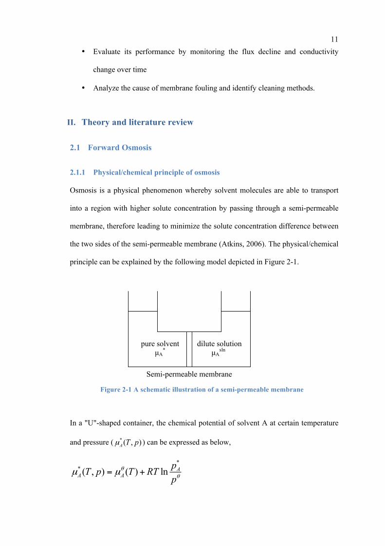
Osmosis is a physical phenomenon whereby solvent molecules are able to transport

into a region with higher solute concentration by passing through a semi-permeable

membrane, therefore leading to minimize the solute concentration difference between

the two sides of the semi-permeable membrane (Atkins, 2006). The physical/chemical

principle can be explained by the following model depicted in Figure 2-1.

In a "U"-shaped container, the chemical potential of solvent A at certain temperature

and pressure ( * ( , )A T pµ ) can be expressed as below,

** ( , ) ( ) ln AA A

pT p T RTp

θθµ µ= +

Figure 2-1 A schematic illustration of a semi-permeable membrane

12 Meanwhile the chemical potential for dilute solution at certain temperature and

pressure ( ln ( , )sA T pµ ) is written as:

ln ( , ) ( ) lns AA A

pT p T RTp

θθµ µ= +

where ( )A Tθµ is the chemical potential of molecules A in the standard state at

temperature of T, *Ap and Ap are the vapor pressure of the pure solvent A and partial

pressure of the solvent A in the dilute solution, respectively.

According to Raoult's law which was established by François-Marie Raoult in 1882,

for an ideal solution, the vapor pressure is proportional to the vapor pressure of each

chemical component (p*A, p*B, p*C...) as well as the mole fraction of the component

existing in the solution (xA, xB, xC...). Thus after the equilibrium for all the

components in the solution is reached, the total vapor pressure p of the solution can be

written as below:

* * * ......A A B B C Cp p x p x p x= + + + ,

and the individual vapor pressure for each component is:

*i i ip p x=

，

where ip is the partial pressure of the component i in the mixture (in the solution),

*ip is the vapor pressure of the pure component i, and ix is the mole fraction of the

component i in the mixture (in the solution).

13 Based on the discussion above, it is not difficult to find that chemical potential of

* ( , )A T pµ > ln ( , )sA T pµ as *

Ap > Ap . Therefore, solvent molecules will move across the

semipermeable membrane from pure solvent side to dilute solution side.

2.1.2 Three kinds of osmotic processes

Osmosis is a physical phenomenon, which is defined as a net movement of water

across a selectively permeable membrane driven by a difference in osmotic pressure

across the membrane.

There are three kinds of osmotic processes (Figure 2-2): reverse osmosis, pressure-

retarded osmosis and forward osmosis (Cath et al., 2006). The general equation of

flux for three processes is:

Jw = A(σ ∆π - ∆P)

Jw is the water flux, A the water permeability constant of the membrane, σ the

reflection coefficient, ∆π the osmotic pressure differential, and ∆P is the applied

pressure.

Figure 2-2 Solvent flows in FO, PRO and RO

14 Source from (Cath et al., 2006)

The arrows show the flux directions of permeating water

Reverse osmosis is commonly used in desalination. Water diffuses to the less saline

side due to applied hydraulic pressure (∆P > ∆π).

Pressure-retarded osmosis (PRO) converts the osmotic pressure into a hydrostatic

pressure, therefore is often used for generating electricity from seawater and fresh

water (Cath et al., 2006). For PRO, water diffuses to the more saline side that is under

positive pressure (∆π >∆P).

Forward osmosis (FO) or osmosis, is a naturally occurring process. The driving force

is the chemical potential difference between two solutions. ∆P is approximately zero

and water diffuses to the more concentrated side of the membrane.

The main advantage of using FO is that it operates at no or low hydraulic pressure,

high rejection of a wide rage of contaminants and lower membrane fouling propensity

than pressure-driven membrane processes (Holloway et al., 2007).

2.2 Forward osmosis mechanism

Water flux though the membrane is related to the difference of chemical potential of

solutions on two sides of the membrane (Cath et al., 2010). The high concentration

solution is called the draw solution. The higher the concentration difference between

draw solution and feed water, the higher the flux is. A lower than expected membrane

flux is often attributed to several membrane-associated transport phenomena.

15 2.2.1 Internal concentration polarization

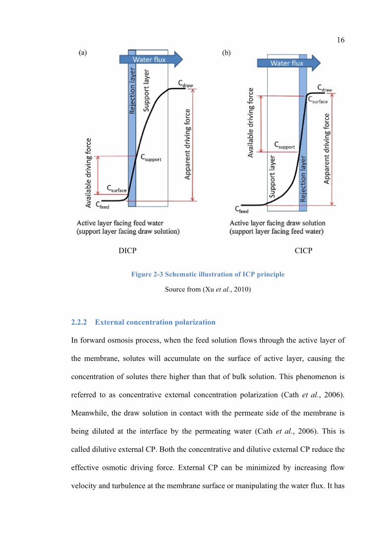
The driving force for osmosis is the concentration difference across the active layer

(Csurface - Csupport), which is called available driving force. The apparent driving force

is the concentration difference between the draw solution and the feed water (Cdraw-

Cfeed) (Xu et al., 2010).

If the active layer is facing the feed water, the solute concentration at the interface of

active layer and support layer is significantly lower than the bulk draw solution

concentration.

Csupport < Cdraw

Csurface ≈ Cfeed

Csupport - Csurface < Cdraw - Cfeed

Therefore, the available driving force is much lower than the apparent driving force.

Water permeates the active layer and dilutes the draw solution within the porous

structure. This is called dilutive internal concentration polarization (DICP) (Gray et

al., 2006).

Similarly, when the feed water is in contact with the porous support layer, there is a

buildup of the solutes at the porous side (Cath et al., 2006).

Csupport > Cfeed

Csurface ≈ Cdraw

Csurface - Csupport < Cdraw - Cfeed

This is called concentrative internal concentration polarization (CICP). The schematic

illustration is shown in Figure 2-3.

16

DICP CICP

Figure 2-3 Schematic illustration of ICP principle

Source from (Xu et al., 2010)

2.2.2 External concentration polarization

In forward osmosis process, when the feed solution flows through the active layer of

the membrane, solutes will accumulate on the surface of active layer, causing the

concentration of solutes there higher than that of bulk solution. This phenomenon is

referred to as concentrative external concentration polarization (Cath et al., 2006).

Meanwhile, the draw solution in contact with the permeate side of the membrane is

being diluted at the interface by the permeating water (Cath et al., 2006). This is

called dilutive external CP. Both the concentrative and dilutive external CP reduce the

effective osmotic driving force. External CP can be minimized by increasing flow

velocity and turbulence at the membrane surface or manipulating the water flux. It has

17 been shown (McCutcheon et al., 2006) that external concentration polarization only

plays a minor role and is not the main reason for flux decline.

2.2.3 FO water flux modeling

The water flux in a forward osmosis process can be modeled by the classical solution-

diffusion model coupled with the diffusion-convection in the membrane support layer

(Tang et al., 2010).

The following derivations comes from (Tang et al., 2010).

Now consider the active layer facing the draw solution (AL-facing-DS). Apply the

solution-diffusion model to the active layer:

( )v draw supportJ A π π= −

( )s draw supportJ B C C= −

where Jv is the volumetric flux of water and Js is the mass flux of solute. Cdraw and

πdraw are the solute concentration and osmotic pressure of the draw solution. Csupport

and πsupport are the solute concentration and osmotic pressure at the interface of FO

support layer and active layer. A is the transport coefficient for water and B is the

transport coefficient for solute.

Consider the solute transport in the support layer, the transport of solute into the

support layer by convection (Jv C) and the part due to the solute back-transport

through the rejection layer (Js) should be balanced by the solute diffusion away from

the support.

18

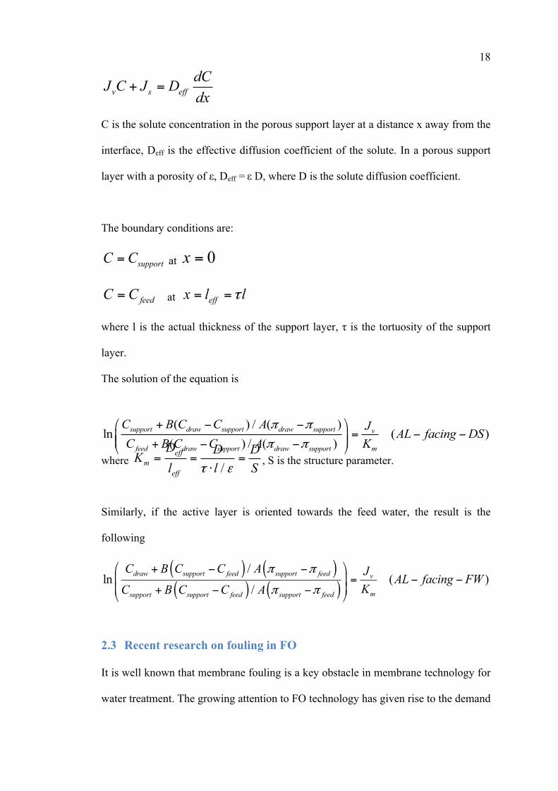
v s effdCJ C J Ddx

+ =

C is the solute concentration in the porous support layer at a distance x away from the

interface, Deff is the effective diffusion coefficient of the solute. In a porous support

layer with a porosity of ε, Deff = ε D, where D is the solute diffusion coefficient.

The boundary conditions are:

supportC C= at 0x =

feedC C= at effx l lτ= =

where l is the actual thickness of the support layer, τ is the tortuosity of the support

layer.

The solution of the equation is

( ) / ( )ln ( )

( ) / ( )support draw support draw support v

feed draw support draw support m

C B C C A J AL facing DSC B C C A K

π π

π π

⎛ ⎞+ − −= − −⎜ ⎟⎜ ⎟+ − −⎝ ⎠

where /eff

meff

D D DKl l Sτ ε

= = =⋅

, S is the structure parameter.

Similarly, if the active layer is oriented towards the feed water, the result is the

following

( ) ( )( ) ( )

/ln ( )

/draw support feed support feed v

msupport support feed support feed

C B C C A J AL facing FWKC B C C A

π π

π π

⎛ ⎞+ − −⎜ ⎟ = − −⎜ ⎟+ − −⎝ ⎠

2.3 Recent research on fouling in FO

It is well known that membrane fouling is a key obstacle in membrane technology for

water treatment. The growing attention to FO technology has given rise to the demand

19 for systematic research on FO membrane fouling for a further understanding of the

FO process and advancing this technology. To date, however, only a few studies (Mi

and Elimelech, 2008) (Mi and Elimelech, 2010) (Lay et al., 2010) (Lee et al., 2010)

(Zou et al., 2011) on solving the problem of FO fouling have been addressed and

reported.

As a powerful tool for interface behavior study, Atomic Force Microscopy (AFM) has

been used to explore the mechanism of FO membrane fouling. Mi and Elimelech

observed a strong correlation between organic fouling and intermolecular adhesion

forces by AFM, using alginate, bovine serum albumin (BSA) and Aldrich humic acid

(AHA) as model organic foulants, as well as quantified intermolecular adhesion

forces between model foulant and the clean or fouled membrane. Their results

suggested that foulant-foulant interaction played an significant role in determining the

rate and extent of organic fouling (Mi and Elimelech, 2008). In their subsequent

work, they examined FO membrane fouling and cleaning behavior by choosing

alginate as a model organic foulant which has been extensively used in membrane

fouling studies. Their results demonstrate that alginate fouling in the FO membrane

process is almost fully reversible through simple physical cleaning (Mi and

Elimelech, 2010).

On the basis of combined experimental and modeling methods, Fane and coworkers

attempted to investigate the fouling propensity of FO by choosing 10-20 nm SiO2

nanoparticles with a concentration of 200 ppm as the model foulant. It was concluded

that factors like low water fluxes, adoption of hydrophilic and smooth membranes as

20 well as the effect of internal concentration polarization could lead to a slower flux

decline phenomenon compared to RO process (Lay et al., 2010).

Lee et al. (Lee et al., 2010) systematically compared the fouling behaviors in FO and

RO processes and further elucidated the fouling mechanisms in FO, using alginate,

humic acid and BSA as model organic foulants, and suspensions of SiO2 colloids with

different sizes as model particulate foulants. Their results indicated that fouling in FO

is almost reversible while irreversible in RO and it was found that the flux decline

behavior in FO could be strongly dependent on various factors including type of

organic foulant, size of colloidal foulant and type of the draw solution selected to

produce the osmotic driving force (Lee et al., 2010). They also pointed out that cake

enhanced osmotic pressure is an important fouling mechanism in FO.

Recent work carried out by Tang and co-workers suggested that some physical and

chemical parameters might play important roles in FO membrane fouling during algae

separation. Their systematic study indicated that more severe FO fouling could be

obtained when adopting greater draw solution concentration and active-layer-facing-

the-draw-solution orientation. Additionally, it was reported that the introduction of

MgCl2 as draw solution could result in significant flux loss when algae were present,

possibly due to the reverse diffusion of Mg2+ from the draw solution into the feed

water (Zou et al., 2011). Mg2+ may have interaction with the foulant on the active

layer such as algae by the effect of charge neutralization or bridging to cause severe

FO fouling.

21 2.4 FO technology

2.4.1 Membranes and modules/ devices

People have done research on forward osmosis membrane even before modern

membrane science has been developed. The following table shows the timeline for FO

membrane development.

Table 2-1 Development of FO membrane

Adapted from (Cath et al., 2006) Time Inventor Material Performance Before 1960s Early membrane

researchers Every type of membrane available including bladders of animals, rubber and goldbeater’ skin

1960s Loeb, Sourirajan and co-workers

Asymmetric aromatic polyamide

1970s All researchers involved

Commercial available RO membranes

Lower flux observed than expected

1990s Osmotek Inc. (Currently HTI)

Cellulose triacetate Higher flux than RO membranes operated in FO mode

Before Hydration Technologies Innovations (HTI) developed a new type of FO

membrane made of cellulose triacetate, researchers used RO membranes operated in

FO mode. The desired properties of FO membrane include the high density of active

layer for high solute rejection and thin support layer with low porosity for low

internal CP.

There are different operating configurations for FO: plate-and-frame, spiral-wound,

tubular, and hydration bags.

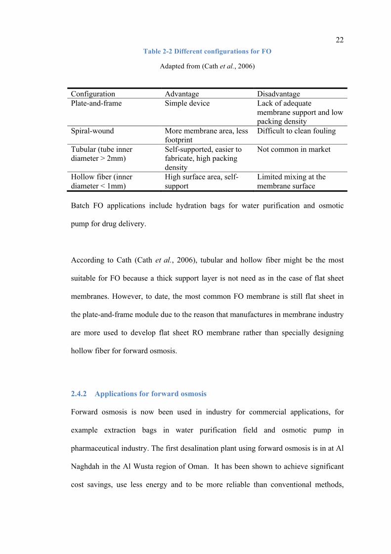
22 Table 2-2 Different configurations for FO

Adapted from (Cath et al., 2006) Configuration Advantage Disadvantage Plate-and-frame Simple device Lack of adequate

membrane support and low packing density

Spiral-wound More membrane area, less footprint

Difficult to clean fouling

Tubular (tube inner diameter > 2mm)

Self-supported, easier to fabricate, high packing density

Not common in market

Hollow fiber (inner diameter < 1mm)

High surface area, self-support

Limited mixing at the membrane surface

Batch FO applications include hydration bags for water purification and osmotic

pump for drug delivery.

According to Cath (Cath et al., 2006), tubular and hollow fiber might be the most

suitable for FO because a thick support layer is not need as in the case of flat sheet

membranes. However, to date, the most common FO membrane is still flat sheet in

the plate-and-frame module due to the reason that manufactures in membrane industry

are more used to develop flat sheet RO membrane rather than specially designing

hollow fiber for forward osmosis.

2.4.2 Applications for forward osmosis

Forward osmosis is now been used in industry for commercial applications, for

example extraction bags in water purification field and osmotic pump in

pharmaceutical industry. The first desalination plant using forward osmosis is in at Al

Naghdah in the Al Wusta region of Oman. It has been shown to achieve significant

cost savings, use less energy and to be more reliable than conventional methods,

23 particularly when operating under challenging conditions. For wastewater reuse

application, it is still under research.

There are only a few articles on the topic of applications in FO and the commercial

applications are still limited as well. In 2006, Cath et al. published an overview of

principles, applications and recent developments of FO technology. In their outlook

they pointed out various possibilities of FO technology used in wastewater

treatment/purification, seawater desalination, food processing, pharmaceutical

industry of osmotic pumps and pressure retard osmosis for power generation. A brief

summary on the applications of wastewater treatment and water purification and

seawater desalination will be given in the following section.

2.4.2.1 Wastewater treatment and water purification

According to the records of the existing documents, in order to develop a possible

method with low energy cost to treat industrial wastewater which contained very low

concentrations of heavy metals for possible reuse, the first bench-scale studies of FO

in an industrial application for wastewater treatment were carried out in the early

1970s by Anderson and his colleagues (Votta et al., 1974) using newly

commercialized cellulose RO membranes to concentrate dilute real or synthetic

wastewater streams containing copper or chromium. However, further pilot-scale

testing of the process was cancelled because of the poor performance of the RO

membranes.

Landfill leachate is liquid that moves through or drains from a landfill, which consists

of four general types of pollutants: organic compounds， dissolved heavy metals,

24 organic and inorganic nitrogen and total dissolved solids (TDS). This liquid may

either already exist in the landfill, or it may be created after rainwater mixes with the

chemical waste. Mechanical evaporation (e.g., vapor compression, vertical tube

falling film, horizontal tube spray film, forced circulation) and membrane processes

are two commercially treatment methods that can efficiently remove TDS from

landfill leachate. A pilot-scale FO system for investigating the concentration of

landfill leachate at the Coffin Butte Landfill in Corvallis (Oregon) was constructed by

Osmotek (Currently HTI), which is considered as a successful example of the pilot-

scale system and starting point to the design and construction of a full-scale system

(Cath et al., 2006).

Except diluted industrial wastewater and landfill leachate, FO is also considered as a

promising process for concentration of centrate which is produced through a sludge

dewatering centrifuge and contains high concentrations of nutrients (e.g.,ammonia,

ortho-phosphate, organic nitrogen), heavy metals, TOC, TDS, color, and TSS. A

meaningful attempt (Holloway et al., 2007) on this process was once carried out by

using a cellulose triacetate FO membrane and a NaCl draw solution at the Truckee

Meadows Water Reclamation Facility (TMWRF) in Reno, Nevada.

2.4.2.2 Seawater desalination

Another important application is seawater desalination. To date, few peer-reviewed

publications and several patents on FO desalination could be found (Cath et al.,

2006). Over the past few decades, desalination of real or simulated seawater with a

batch scale for emergency water supply was investigated, rather than a continuous

25 process for seawater desalination.

By adopting a mixture of highly soluble ammonia and carbon dioxide gases as strong

draw solution, recent studies based on bench scale testing demonstrated that seawater

could be efficiently desalinated through a suitable FO membrane (McCutcheon et al.,

2006). Salt rejections up to 95% and fluxes as high as 25 L/(m2h) with the FOCTA

membrane (McCutcheon et al., 2005) were reported, but much greater flux is actually

expected for such a high driving force. However, it is still widely believed that two

critical drawbacks, i.e., low performance FO membrane and not easily separable draw

solution, could limit its further application.

2.5 Sequential Batch Reactor

A sequential batch operation consists of filling, aeration, settling, decantation and

idling phases in the same reactor. As a result of recent regulations on nutrient

discharges to surface waters, sequential batch reactors have been modified to achieve

nitrogen removal in addition to COD and phosphate (Chang et al., 2000), (Kargi and

Uygur, 2004). The operation phase consists of anaerobic, anoxic and oxic (aerobic)

phases when nutrient removal from the wastewater is desired (Metcalf and Eddy,

1991).

In a sequential batch reactor, the same reactor is used for biological oxidation and

sedimentation. SBR has a smaller footprint and also has the ability of accommodating

a variable incoming flow.

26 2.6 Membrane Bioreactor

Membrane bioreactors (MBR) have gradually become more prevalent as a wastewater

treatment process. MBR eliminates the sedimentation tank and uses a submerged

membrane module in the reaction basin.

One difference between SBR and MBR is the flow mode. The process of MBR is

continuous influent and continuous effluent, while SBR does not have continuous

input and output.

SBR can have a higher flow capacity when operated in a parallel unit. Also SBR is

more robust in terms of resistance to high concentration peaks or toxic wastewater

(Tchobanoglous et al., 2003)

2.7 Fouling in MBR

While there was only limited research on FO fouling, there are already many papers

published on the fouling in MBR. In our study we combine microbial process with FO

membrane in the same tank, which is similar to MBR. Therefore, previous results on

fouling in MBR could give us guidance and insight in our study.

2.7.1 Fouling mechanism

Fouling refers to undesirable accumulation of materials on the internal or external

structure of a membrane. These materials may include particles, colloids, and organic

molecules. If microorganisms or other kinds of living things are involved, we may use

the term biofouling (Le-Clech et al., 2006).

Biofouling has a significant impact on membrane performance. In any membrane

process, three basic aspects determine the degree of fouling: the nature of the feed, the

27 membrane properties and the hydrodynamic operating environment (Zhang et al.,

2006). The more detailed factors are listed in Figure 2-4.

Figure 2-4 The fouling mechanism

Source from (Zhang et al., 2006)

28

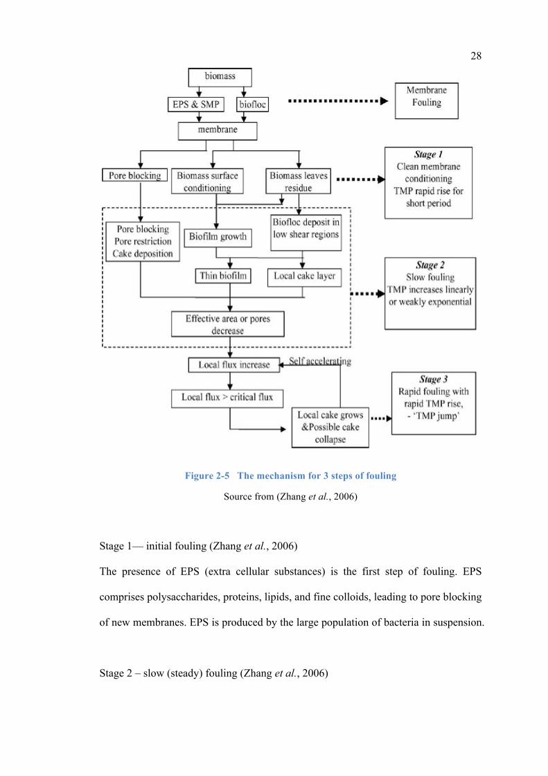
Figure 2-5 The mechanism for 3 steps of fouling

Source from (Zhang et al., 2006)

Stage 1— initial fouling (Zhang et al., 2006)

The presence of EPS (extra cellular substances) is the first step of fouling. EPS

comprises polysaccharides, proteins, lipids, and fine colloids, leading to pore blocking

of new membranes. EPS is produced by the large population of bacteria in suspension.

Stage 2 – slow (steady) fouling (Zhang et al., 2006)

29 The biofilm growth is steady even with a good hydrodynamic environment that

provides adequate surface shear over the membrane surface. However, heavy local

fouling will occur when there is maldistribution of flow, shear or flux.

Stage 3 – The TMP jump (Zhang et al., 2006)

When MBR is operated in constant pressure mode, fouling causes flux decline and

fouling is self-limiting. If operated in constant flux mode, fouling is self-accelerating.

2.7.2 Mitigation of MBR fouling

2.7.2.1 Physical cleaning

Physical cleaning methods for MBR include membrane backwashing and membrane

relaxation. These methods are routinely used and therefore are incorporated in most

MBR designs (Le-Clech et al., 2006).

Backwashing is also called back flushing. It can remove most of the reversible fouling

due to pore blocking. The design parameters for backwashing are frequency, duration

and intensity.

Membrane relaxation means that the membrane is in operation intermittently rather

than continuously. During the relaxation time, the foulants on the membrane can

diffuse away through the concentration gradient. The membrane productivity will

increase more significantly if air scouring is applied during relaxation (Chua et al.,

2002).

30 2.7.2.2 Chemical cleaning

The effectiveness of physical cleaning methods tends to decrease with time as more

irreversible fouling accumulates on the membrane surface. Therefore, chemical

cleaning should be applied to the membrane when the flux decline is severe. The

chemical cleaning includes: chemically enhanced backwash (on a daily basis),

maintenance cleaning with higher chemical concentration (weekly) and intensive

chemical cleaning (once or twice a year).

The main MBR suppliers have their own chemical cleaning recipes, which differ with

respect to concentrations and methods. However, for organic foulants, the prevalent

cleaning agents remain sodium hypochlorite, and for inorganic foulants, citric acid is

commonly used.

Sodium hypochlorite can remove organic foulants by hydrolyzing the organic

molecules and therefore loosen the particles and biofilm attached to the membrane.

Lim et al. (Lim et al., 2005) also studied the effect of sodium hypochlorite on the

microbial community. They pointed out the organic degradation performance of the

microbial community was impaired in the presence of sodium hypochlorite due to cell

lysis.

2.8 Nitrogen removal in water treatment

2.8.1 Biological process

In water, elemental nitrogen can be in the form of nitrate, nitrite, ammonia and

organic nitrogen.

31 All of the biological nitrogen removal processes include an aerobic zone where

biological nitrification occurs.

Denitrification is the process of nitrate reduction via nitrite, nitric oxide, nitrous oxide

to nitrogen. In this process, nitrate works as electron acceptor and the available

organic carbon in the wastewater works as electron donor. Heterotrophic bacteria

(denitrifier) are involved in this process.

Denitrification is a pathway of nitrogen loss. It plays an important role in nutrient

cycling. In terms of the general nitrogen cycle, denitrification completes the cycle by

returning N2 to the atmosphere. Factors that can help reduce nitrogen losses via

denitrification include microbial conversion of inorganic N to organic forms, low

rates of nitrification, high C: N of the source material and inhibition due to the

presence of toxic metabolites (Alongi, 1998). Some other factors influencing

denitrification rates are oxygen supply, temperature, nitrate levels, pH, enzyme

activity and enzyme quantity.

The SBR system employs preanoxic denitrification using BOD in the influent

wastewater. Mixing is used to contact the mixed liquor with the influent wastewater.

For many domestic applications, depending on the wastewater strength, sufficient

BOD and fill time are available to remove almost all the nitrate remaining in the

mixed liquor after the settle and decant steps. Some nitrate removal also occurs during

the nonaerated settle and decant periods (Tchobanoglous et al., 2003)

32

III. Materials and methods

3.1 Materials

3.1.1 Sample water

3.1.2 SWW (Synthetic waste water)

The synthetic wastewater was used to mimic pre-settled domestic wastewater. The

recipe was adapted from Nopens et al., (2001). The calculated COD, N and P are

439.47 mg/L, 60.23 mg/L and 9.42 mg/L, respectively. The detailed recipe is in the

appendix. In order to save the time for preparing the SWW, we prepared a stock

solution (called concentrated SWW), which is ten times the concentration of SWW.

3.1.3 Synthetic inorganic solution

Synthetic inorganic solution is used to dilute concentrated SWW to adjust the

conductivity of the feed water in the tank. The aim is to establish the conductivity of

feed at a certain value. The recipe is in show in the appendix.

3.1.4 FO membranes

Hydration Technology Innovations (HTI) supplied FO membranes for this study.

The membrane we used is in the cartridge product, which has a higher flux but a

lower salt rejection when compared to the membrane in the pouch product.

The cartridge membrane is prepared by coating cellulose triacetate onto a polyester

screen mesh. The active layer is to the inside of the roll and is the shiny side; on

drying, the membrane will curl towards the rejection layer. The thinner membrane

support layer can minimize internal concentration polarization, which can be proved

by the theoretical model for ICP and FO flux.

33 The dehydrated (compacted) membrane will not transfer water and cannot be fixed. A

similar phenomenon can occur by exposing one side to concentrated brine and

nothing on the other side. Flux losses of 50% or more can be observed.

Orientation of the membrane makes a big difference in the distilled water versus draw

solution test. Fluxes will always be higher when the draw solution is on the active

layer side of the membrane.

FO membranes behave similarly to RO membranes in that dissolved gases are not

rejected well. Their ions are rejected, but the (often small) fraction that exists as a

dissolved gas is not rejected. Small polar, water-soluble organics, such as urea,

methanol, and ethanol, are also not rejected well. There may be a transfer of the draw

solution ions or molecules if they are very small.

3.1.5 Alconox cleaning solution

The cleaning solution for RO elements containing cellulose triacetate (CTA)

membrane is presented in Table 3-1. We adapted a similar cleaning solution for our

FO CTA membrane, shown in Table 3-2.

Table 3-1 Chemical cleaning solution for RO elements with CTA membrane

Chemical Concentration (g/L)

Trisodium phosphate 20

Sodium EDTA powder 8

Triton X-100 1

34 Table 3-2 Chemical cleaning solution for FO membrane

Chemical Concentration (g/L)

Alconox* 10

Sodium EDTA powder 8

*The ingredients of Alconox are in the Table 3-3.

Table 3-3 Ingredients for Alconox

Ingredient name Concentration%

Sodium dodecylbenzenesulfonate 10-30

Sodium carbonate 7-13

Tetrasodium pyrophosphate 10-30

Sodium phosphate 10-30

http://www.alconox.com/downloads/pdf/msds_alconox_english_eu.pdf

35 3.1.6 Analytical equipment and methods

3.1.6.1 Zeta potential analyzer

Figure 3-1 Electro Kinetic Analyzer

The Zeta potential (membrane charge) of the membrane was measured using an

Electro Kinetic Analyzer (SurPASS) equipped with a clamping cell.

A 10 mM KCl solution was used as background electrolyte. The pH was adjusted

automatically with 0.1 M HCl and 0.1 M NaOH to various values during the analysis.

36 3.1.6.2 Theta Optical Tensiometer

Figure 3-2 Theta Optical Tensiometer

The contact angle was measured by Theta Optical Tensiometer from KSV instrument.

The sample membrane was attached to the sample stage. A drop of 5 µl of MQ water

was placed from the syringe and the image was recorded with time. After curve fitting

of the recorded images, the contact angle was calculated.

3.1.6.3 ATP Analyzer

ATP analyzer is from Celsis Advanced Luminometer.

37

Figure 3-3 ATP analyzer

Active biomass was determined in duplicate by measuring the adenosine-

triphosphate (ATP) concentration in 50 µL samples (Holm-Hansen and Booth, 1966).

The amount of light produced was measured with the luminometer (relative light

units). The concentration of ATP was derived from the relative light units (RLU)

value using the conversion factors of a calibration curve between relative light units

(RLU) values and reference ATP concentrations.

We used this equipment to analyze the foulant layer of the membrane. A membrane

coupon with a (3cm x 3cm) foulant layer was scrubbed gently. The folants were

dissolved in DI water. After homogenizing the foulants with a sonicator and a vortex

mixer, the foulants were distributed well and the prepared sample could be tested

(Vrouwenvelder, 2009).

38 3.1.6.4 Microscope

Figure 3-4 Microscope

Samples were prepared according to different requirements. If we were going to

observe transparent exopolymer particles (TEP) on the membrane, a type of dye

Alcian Blue was used to make TEP visible, turning them into blue spots. Then the

prepared membranes were put on a glass slide with the cover glass on top. There were

four different lenses. We started from the low magnification lens. The focus was

adjusted until a clear image was observed.

3.1.6.5 Fluorescence Excitation-emission matrix spectroscopy

39

Figure 3-5 F-EEM Spectroscopy

Fluorescence Excitation-emission matrix spectroscopy (F-EEM) is a valuable tool in

water quality monitoring, based on identifying fluorescence emitting organic

substances (fluorophores) present in water systems. Humic-like, protein-like and

xenobiotic-like fluorophores can be identified from EEMs and could be clearly

differentiated based on their fluorescing composition. At low concentrations the

flurescence intensity will generally be proportional to the concentration of the

fluorophore.

Table 3-4 Peak position of F-EEM

Peak description Fluorescence Range Excitation (nm) Emission (nm)

Humic-like (Primary) 330-350 420-480 Humic-like (Secondary) 250-250 380-480 Protein-like (Tyrosine) 270-280 300-320

Protein-like (Tryptophan) 270-280 320-350 Protein-like (Albumin) 280 320

Table 3-5 Methods of scanning

Target compounds Humic-like Protein-like Excitation wavelength λex 340 nm 270 nm

Emission range λem 370-700 nm 300-700 nm Strongest emission λem-max About 440 nm About 340 nm

Rayleigh second order scattering * About 680 nm About 540 nm *According to (Huang et al., 2010)

40 3.1.6.6 LC-OCD

Figure 3-6 LC-OCD

LC-OCD stands for Liquid Chromatography - Organic Carbon Detection. Apart from

OCD, there is also a UV-detector and an organic nitrogen detector (OND).

Mechanism: Due to a size exclusion chromatography column, different components

are separated on the basis of molecular size. When molecules are diffusing through

into the resin pores, the larger molecules exit earlier as they are not able to penetrate

the pores very deeply. Similarly, the small molecules can penetrate the pores better

and reside for a longer time in diffusing through the column.

41

Biopolymers: Polysaccharides, Proteins, Aminosugars

Building blocks: mostly breakdown products of humics Acids: summaric value for monoprotic organic acids < 350 Da Neutrals: mono-oligosaccharides, alcohols, aldehydes, ketones and amino sugars

Table 3-6 The eluting sequence for LC-OCD

Compounds Retention time Hydrophobic bypass 0-20 min Biopolymers 26-38 min Humics 40-46 min Building blocks 46-53 min Acids 53-57 min LMW neutrals After 60 mins

Figure 3-7 LC-OCD graph interpretation

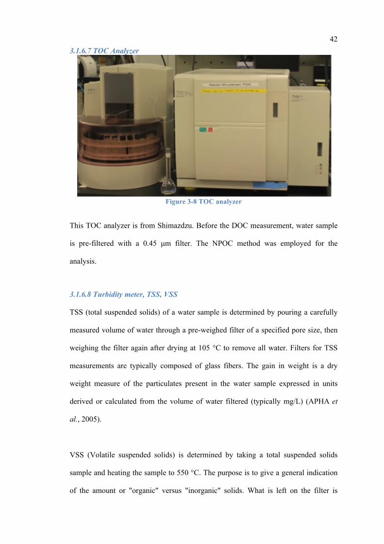
42 3.1.6.7 TOC Analyzer

Figure 3-8 TOC analyzer

This TOC analyzer is from Shimazdzu. Before the DOC measurement, water sample

is pre-filtered with a 0.45 µm filter. The NPOC method was employed for the

analysis.

3.1.6.8 Turbidity meter, TSS, VSS

TSS (total suspended solids) of a water sample is determined by pouring a carefully

measured volume of water through a pre-weighed filter of a specified pore size, then

weighing the filter again after drying at 105 °C to remove all water. Filters for TSS

measurements are typically composed of glass fibers. The gain in weight is a dry

weight measure of the particulates present in the water sample expressed in units

derived or calculated from the volume of water filtered (typically mg/L) (APHA et

al., 2005).

VSS (Volatile suspended solids) is determined by taking a total suspended solids

sample and heating the sample to 550 °C. The purpose is to give a general indication

of the amount or "organic" versus "inorganic" solids. What is left on the filter is

43 basically inorganic. What "volatilizes" is organic.

Turbidity

Turbidity is an optical characteristic or property of a liquid. The value of turbidity is

related to the loss of transparency, caused by the presence of suspended particles and

colloids. A liquid that has few suspended materials inside is more clear, thus having a

low value of turbidity.

The turbidimeter we used is HACH 2100 AN.

3.1.6.9 COD, Ammonia, Nitrate, Nitrite, Total Nitrogen, Total Phosphate These parameters were measured with HACH measuring kits. The product series are

listed below.

Ammonia

DOC 316.53.01079

Salicylate Method Method 10031

Instrument DR 2800

COD DOC 316.53.01099

USEPA Reactor Digestion method Method 8000

Nitrate DOC 316.53.01068

Chromotropic acid method Method 10020

Nitrite DOC 316.53.01075

Ferrous Sulfate Method Method 8153

44 3.2 Experimental methods

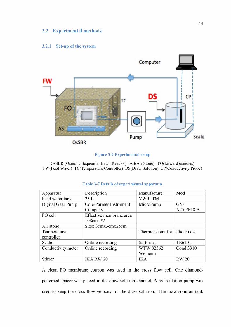
3.2.1 Set-up of the system

Figure 3-9 Experimental setup

OsSBR (Osmotic Sequential Batch Reactor) AS(Air Stone) FO(forward osmosis) FW(Feed Water) TC(Temperature Controller) DS(Draw Solution) CP(Conductivity Probe)

Table 3-7 Details of experimental apparatus

Apparatus Description Manufacture Mod Feed water tank 25 L VWR TM Digital Gear Pump Cole-Parmer Instrument

Company MicroPump GY-

N25.PF18.A FO cell Effective membrane area

108cm2 *2

Air stone Size: 3cmx3cmx25cm Temperature controller

Thermo scientific Phoenix 2

Scale Online recording Sartorius TE6101 Conductivity meter Online recording WTW 82362

Weiheim Cond 3310

Stirrer IKA RW 20 IKA RW 20 A clean FO membrane coupon was used in the cross flow cell. One diamond-

patterned spacer was placed in the draw solution channel. A recirculation pump was

used to keep the cross flow velocity for the draw solution. The draw solution tank

45 contains filtered Red Sea water initially. A digital scale connected to a computer data

logging system is put below the draw solution tank to monitor the permeate water flux

from the FO cell. In addition, an online conductivity is also used to monitor the

conductivity decline of the draw solution with time.

The feed water tank was filled with wastewater with activated sludge, and the FO cell

was immersed in the feed water tank. For a typical FO experiment, the pH,

conductivity and volume of feed water is adjusted to be the same at the beginning of

each cycle.

Temperature: 20 °C

Pump flow: 70 mL/min

Air stone flow: 5 L/min

Membrane orientation: If not mentioned in particular, the active layer is facing the

feed water in the tank, and the support layer is facing the draw solution.

3.2.2 General procedure of experiments

3.2.2.1 Start-up phase

The main purpose of the start-up phase is to incubate microbes for SBR. Raw

domestic wastewater after primary treatment was collected on KAUST campus. 1L

of wastewater was mixed with 19 L of synthetic wastewater. After 2 days of aeration,

5 L of supernatant was removed and replaced by 5 L of mixture of SWW and raw

domestic wastewater. After repeating the 2-day cycles for 3 weeks, the TSS was 606

mg/L and the VSS was 513 mg/L (data of March 27). Although the TSS and VSS

46 values were still lower than the normal standard in domestic wastewater treatment

plant, these values were adequate to start Osmotic SBR process.

3.2.2.2 Stable cycle

The wastewater was treated by two modes. Seawater was employed as the draw

solution and circulated in the FO cell to recover the fresh water from the wastewater.

Mode 1 was conducted by three steps, i.e. aeration, sedimentation and FO decantation

without air scouring. Mode 2 (i.e., aeration followed by FO decantation with air

scouring) could attain better water flux than mode 1. In Mode 2, the air flow rate is 5

L/min. As the volume of the feed water in the tank is 25 L, the air water ratio is 12

L/h air /(L feed water).

Decantation with air scouring could reduce the fouling on the membrane surface,

consequently, enhancing the flux of FO. As a sequential batch reactor, each cycle

lasted for 1 day. Fresh seawater was placed as draw solution each day. The feed water

in tank was adjusted by the synthetic wastewater and inorganic solution to keep the

conductivity constant. All these cycles were operated with one membrane

sequentially. The detailed operational parameters are listed in Table 3-8.

Table 3-8 Two operation modes for OsSBR

* Idle time is used for sedimentation, removing effluent and refilling.

Mode 1 Mode 2 Aeration 6 hour 8 hour Sedimentation 2 h 0 FO decantation 15h without air scouring 15h with air scouring Idle time for refilling * 1 h 1 h TSS of feed water < 700 mg/L 1000 mg/L

47 3.2.2.3 Cleaning methods

We used three different approaches of cleaning. They were applied to the same

membrane sequentially, rather than in parallel.

Chemical cleaning of the active layer

The cleaning solution is 10 g/L Alconox and 8 g/L Sodium EDTA. The membrane

cell was immersed in the cleaning solution horizontally without extra turbulence with

20 minutes for each side.

Osmotic Backwash to clean the active layer

The principle of backwash is to change the water flow direction by changing the

concentration gradient. Therefore the accumulated foulants on the active layer can be

washed away by the water flux coming from the support layer. The FO cell was

immersed in seawater. DI water was circulated inside the cell to keep in contact with

the support layer. The pump flow was 70 mL/min. After 7 hours of osmotic backwash,

a test with DI feed was conducted to evaluate the cleaning effect.

Cleaning the support layer of the membrane

1) Cleaning solution: 1% of NaClO (sodium hypochlorite)

The conductivity of the cleaning solution was 31.7 mS/cm and pH was 8. We used DI

as feed water and 1 L of NaClO solution as draw solution. NaClO solution was

circulated inside the cell at the flow of 100 mL/min for 25 minutes.

2) Cleaning solution: 10 g/L Alconox and 8 g/L sodium EDTA

48 The conductivity of the cleaning solution was 9.5 mS/cm. We used DI as feed water

and 600 ml of Alconox and sodium EDTA solution as draw solution. Alconox and

sodium EDTA solution was circulated inside the cell at the flow of 150 mL/min for

10 minutes. After cleaning, DI water was used to rinse the inside of the cell at the

flow of 300 mL/min for 20 minutes.

49

IV. Results and discussion

4.1 Membrane characterization

4.1.1 Contact angle

The contact angle measurement was used to indicate the hydrophilicity/

hydrophobicity of a membrane surface.

For measuring contact angle, we tried two types of attachment for the membranes

using one side tape and Double- sided tape respectively. The data show that the

contact angle with Double- sided tape is 20 degree less than one side tape.

Three types of membrane were tested. The first type of membrane was virgin

membrane. The second one was fouled membrane. And the third one was fouled

membrane after cleaning (by scrubbing gently).

The results are shown in Table 4-1. We can get the sequence of contact angle: Fouled

membrane after cleaning > Virgin membrane > Fouled membrane.

This shows that the fouled membrane is more hydrophilic than the virgin membrane.

Table 4-1 Contact angle results for HTI membrane

Attachment type: One side tape

Attachment type: Double-sided tape

Virgin membrane 68.1 ± 1.8 ---- Fouled membrane 56.6 ± 3.3 37.9 ± 3.7

Fouled membrane after cleaning 72 ± 1.6 50.0 ± 2.1

50 4.1.2 Zeta potential

The zeta potential (surface charge) of the FO membrane changed after fouling. Both

the virgin membrane and the fouled membrane were tested for both the active layer

and the support layer. The fouled membrane was operated for three months. Within

the three months, different cleaning methods were used. The results are shown in

Figure 4-1 and Figure 4-2.

Figure 4-1 shows that there were more negative surface charges on the active layer of

the fouled membrane than the virgin membrane at pH > 6. But for the surpport layer,

the surface charge of the fouled membrane was greater than the virgin membrane in

all pH range (Figure 4-1).

Figure 4-1 Zeta potential of active layer

51

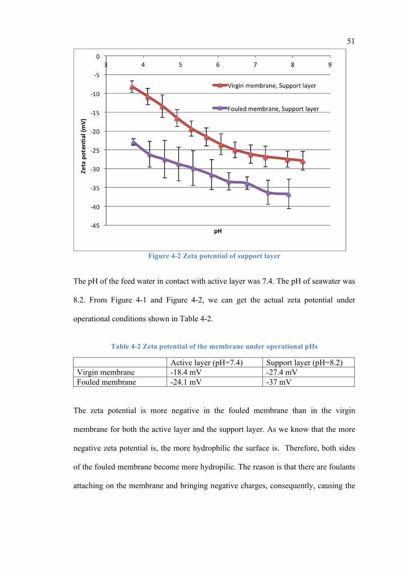
Figure 4-2 Zeta potential of support layer

The pH of the feed water in contact with active layer was 7.4. The pH of seawater was

8.2. From Figure 4-1 and Figure 4-2, we can get the actual zeta potential under

operational conditions shown in Table 4-2.

Table 4-2 Zeta potential of the membrane under operational pHs

Active layer (pH=7.4) Support layer (pH=8.2) Virgin membrane -18.4 mV -27.4 mV Fouled membrane -24.1 mV -37 mV

The zeta potential is more negative in the fouled membrane than in the virgin

membrane for both the active layer and the support layer. As we know that the more

negative zeta potential is, the more hydrophilic the surface is. Therefore, both sides

of the fouled membrane become more hydropilic. The reason is that there are foulants

attaching on the membrane and bringing negative charges, consequently, causing the

52 zeta potential to be more negative. For example, biopolymers which have carboxylic

groups can contribute to this phenomenon.

4.2 Water characterization

4.2.1 TOC/DOC

Four different types of water were measured. Table 4-3 shows the results.

Synthetic wastewater (SWW) was fed in the tank every day.

Batch reactor effluent (BRE) was collected in the wastewater tank after aeration and

sedimentation.

Diluted draw solution (DDS) was collected in the draw solution tank after 15 hours of

dilution. Three different DDS were collected under different scenarios.

DDS 4-5 was collected on April 5th. The feed water was wastewater in tank and the

membrane was fouled. It is worth noting that the PVC tubings that connect the cell

and draw solution were biofouled seriously.

DDS 6-2 was collected on June 2nd. The feed water was wastewater in tank and the

membrane were fouled. The previous biofouled PVC tubings were replaced and clean

silicone tubings were used.

DDS 6-6 was collected on June 6th. The feed water was DI water. This DDS was

taken at the second day of operation for a new membrane.

Seawater (SW) was from the Red Sea and filtered by a 0.45 µm filter. This was used

as the draw solution.

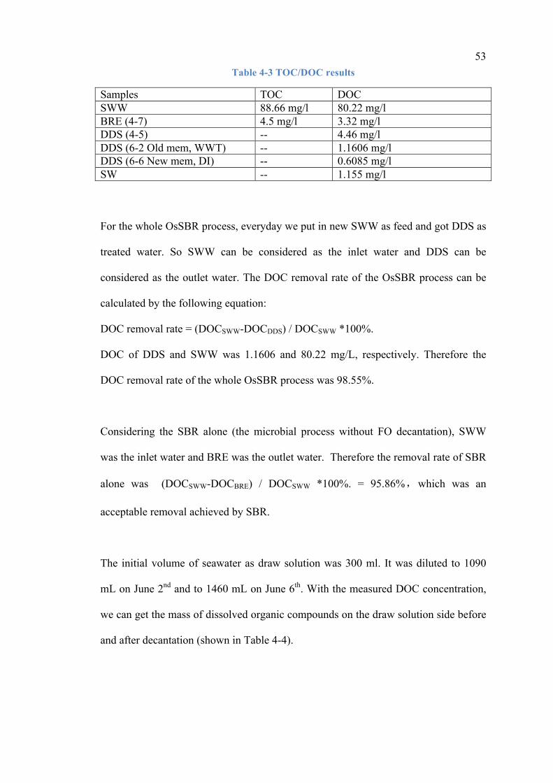
53 Table 4-3 TOC/DOC results

Samples TOC DOC SWW 88.66 mg/l 80.22 mg/l BRE (4-7) 4.5 mg/l 3.32 mg/l DDS (4-5) -- 4.46 mg/l DDS (6-2 Old mem, WWT) -- 1.1606 mg/l DDS (6-6 New mem, DI) -- 0.6085 mg/l SW -- 1.155 mg/l

For the whole OsSBR process, everyday we put in new SWW as feed and got DDS as

treated water. So SWW can be considered as the inlet water and DDS can be

considered as the outlet water. The DOC removal rate of the OsSBR process can be

calculated by the following equation:

DOC removal rate = (DOCSWW-DOCDDS) / DOCSWW *100%.

DOC of DDS and SWW was 1.1606 and 80.22 mg/L, respectively. Therefore the

DOC removal rate of the whole OsSBR process was 98.55%.

Considering the SBR alone (the microbial process without FO decantation), SWW

was the inlet water and BRE was the outlet water. Therefore the removal rate of SBR

alone was (DOCSWW-DOCBRE) / DOCSWW *100%. = 95.86%，which was an

acceptable removal achieved by SBR.

The initial volume of seawater as draw solution was 300 ml. It was diluted to 1090

mL on June 2nd and to 1460 mL on June 6th. With the measured DOC concentration,

we can get the mass of dissolved organic compounds on the draw solution side before

and after decantation (shown in Table 4-4).

54 Table 4-4 Mass balance for draw solution side

SW DDS 6-2 DDS 6-6 DOC (mg/l) 1.155 1.1606 0.6085 Volume (ml) 300 1090 1460 Mass (µg) 346.5 1265 888

The data from Table 4-4 shows that after decantation, there were more organic

compounds on the draw solution side. Considering DDS 6-6, there was no DOC in the

feed water (DI), the increased DOC mass should have come from the glycerin,

preserving the membrane. As this was only the second day of operation for the new

membrane, it is understandable that some preserving organic residuals were coming

from the membrane, which were used for preservation of the membrane.

For DDS 6-2, there are more organic compounds in the draw solution side than DDS

6-6. The increased mass may come from the feed water, considering that the

membrane, which had been operated for three months, was already without residues

of the preservatives.

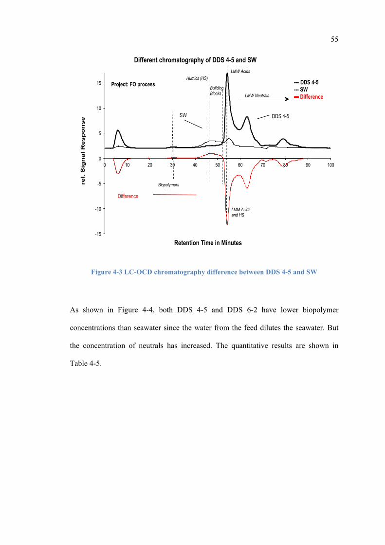
4.2.2 LC-OCD The DDS sample was taken on April 5th. There were no building blocks in seawater.

Figure 4-3 shows that the FO membrane has good effects on rejecting high molecular

weight compounds such as biopolymers and humics substrates. But the concentration

of LMW acids (< 350 Dalton) increased significantly in DDS compared to SW. This

indicates that FO does not work effectively in rejecting low MW molecules that are

less than 350 Dalton (Figure 4-3).

55

-15

-10

-5

0

5

10

15

0 10 20 30 40 50 60 70 80 90 100

rel. S

ign

al R

es

po

ns

e

Retention Time in Minutes

Different chromatography of DDS 4-5 and SW

Biopolymers

Humics (HS)

Building Blocks

LMM Acids and HS

LMW Neutrals

Project: FO process

SW

--- DDS 4-5 --- SW

Difference

DDS 4-5

Difference

LMW Acids

Figure 4-3 LC-OCD chromatography difference between DDS 4-5 and SW

As shown in Figure 4-4, both DDS 4-5 and DDS 6-2 have lower biopolymer

concentrations than seawater since the water from the feed dilutes the seawater. But

the concentration of neutrals has increased. The quantitative results are shown in

Table 4-5.

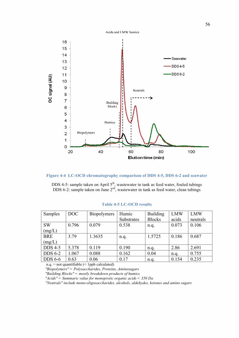
56

Figure 4-4 LC-OCD chromatography comparison of DDS 4-5, DDS 6-2 and seawater

DDS 4-5: sample taken on April 5th, wastewater in tank as feed water, fouled tubings DDS 6-2: sample taken on June 2nd, wastewater in tank as feed water, clean tubings

Table 4-5 LC-OCD results

Samples DOC Biopolymers Humic Substrates

Building Blocks

LMW acids

LMW neutrals

SW (mg/L)

0.796 0.079 0.538 n.q. 0.073 0.106

BRE (mg/L)

3.79 1.3635 n.q. 1.5725 0.186 0.687

DDS 4-5 5.378 0.119 0.190 n.q. 2.86 2.691 DDS 6-2 1.067 0.088 0.162 0.04 n.q. 0.755 DDS 6-6 0.63 0.06 0.17 n.q. 0.154 0.235 n.q. = not quantifiable (< 1ppb calculated) "Biopolymers" = Polysaccharides, Proteins, Aminosugars "Building Blocks" = mostly breakdown products of humics "Acids" = Summaric value for monoprotic organic acids < 350 Da

"Neutrals" include mono-oligosaccharides, alcohols, aldehydes, ketones and amino sugars

57

DDS 6-2: sample taken on June 2nd, wastewater in tank as feed water, clean tubings

DDS 6-6: sample taken on June 6th, DI as feed water, new membrane

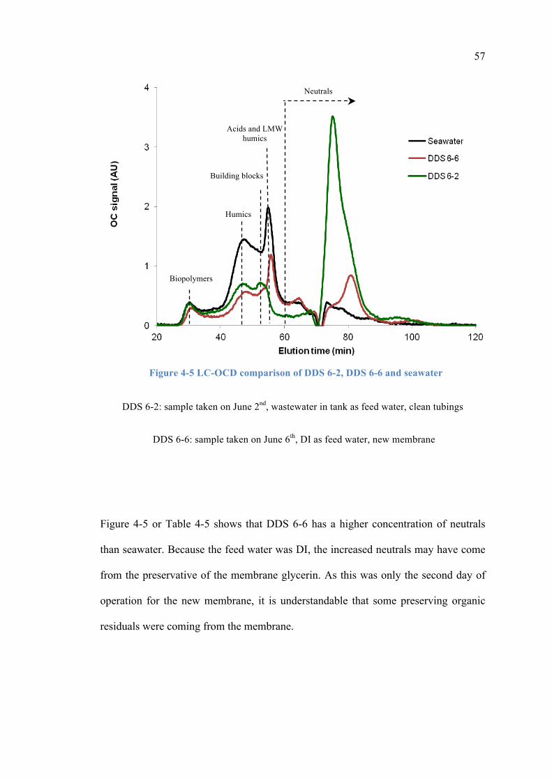
Figure 4-5 or Table 4-5 shows that DDS 6-6 has a higher concentration of neutrals

than seawater. Because the feed water was DI, the increased neutrals may have come

from the preservative of the membrane glycerin. As this was only the second day of

operation for the new membrane, it is understandable that some preserving organic

residuals were coming from the membrane.

Building blocks

Humics

Acids and LMW humics

Biopolymers

Neutrals

Figure 4-5 LC-OCD comparison of DDS 6-2, DDS 6-6 and seawater

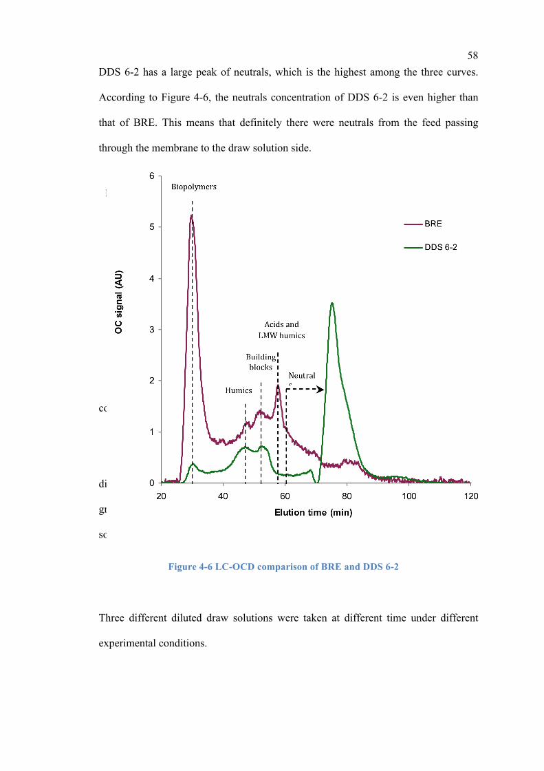
58 DDS 6-2 has a large peak of neutrals, which is the highest among the three curves.

According to Figure 4-6, the neutrals concentration of DDS 6-2 is even higher than

that of BRE. This means that definitely there were neutrals from the feed passing

through the membrane to the draw solution side.

BRE: batch reactor effluent

DDS 6-2: sample taken on June 2nd, wastewater in tank as feed water,

clean

tubings

4.2.3 F-EEM

In order to determine the

performance of the FO

membrane in rejecting the

compounds from the feed water, we

compared the

concentrations of

different

group of compounds between seawater and diluted draw

solution using F-EEM.

Three different diluted draw solutions were taken at different time under different

experimental conditions.

Figure 4-6 LC-OCD comparison of BRE and DDS 6-2

59 One sample, DDS 4-5, was taken when the membrane was fouled after one month in

wastewater tank. The PVC tubes connecting the membrane cell and seawater were

biofouled.

The second diluted draw solution, DDS 6-2, was also taken when the membrane was

fouled. But it was taken after the fouled PVC tubings were replaced with silicone

tubings. So the difference of the first DDS and second DDS shows the contamination

of the fouled tubings.

The third sample, DDS 6-6, was taken when a virgin membrane was operated after

the second 15 hours cycle. The results of DDS 6-6 can show the effect of a

preservative compound (glycerin). The difference between results of DDS 6-2 and

DDS 6-6 can indicate the real effect of the feed water.

In DDS 4-5 (Figure 4-7), there is a peak at excitation 275, emission 325 nm. It shows

the protein-like organic matter (tryptophan). There is an increase in the concentration

of proteins from the seawater to the diluted draw solution. As we know, proteins are

generally too big to pass through the FO membrane, they were originated from the

biofouling of the tubings. Two pictures of different fouling tubings are shown in

Figure 4-8.

60

DDS 4-5: sample taken on April 5th, wastewater in tank as feed water, fouled tubings

Figure 4-8 Fouling of tubings

Figure 4-9 shows three water samples according to the same scale of intensity.

Comparing SW, DDS 6-2, and DDS 6-6, the humics peaks vanish in DDS 6-6 and in

DDS 6-2. This indicates that humics are rejected quite well by the FO membrane.

This is constant with the results of LC-OCD. The concentrations of humic substances

in DDS are much lower than that of seawater.

300 350 400 450 500

250

300

350

400

450

Emission Wavelength (nm)

Exc

itatio

n W

avel

engt

h (n

m)

0.000

4375

8750

1.313E+04

1.750E+04

2.188E+04

2.625E+04

3.063E+04

3.500E+04

300 350 400 450 500

250

300

350

400

450

Emission Wavelength (nm)

Exc

itatio

n W

avel

engt

h (n

m)

0.000

4375

8750

1.313E+04

1.750E+04

2.188E+04

2.625E+04

3.063E+04

3.500E+04

SW DDS 4-5

Figure 4-7 F-EEM comparison of SW and DDS 4-5

61

Comparing DDS 6-2 with SW (Figure 4-9), we can also see an increase in the bottom

showing green (emission 350 nm, excitation 240 nm), since the excitation-emission

wavelength is not in the identifying range of the F-EEM, we could not identify what it

was.

Comparing DDS 6-6 and SW (Figure 4-9), we could see the concentration of most

compounds decrease except a small part in the left-bottom corner. This might be due

to the leaching of preservative from the new membrane, as it is just the second day of

operation. According to previous result, there might be glycerin leaching from the

membrane.

62

Figure 4-9 F-EEM comparison of SW, DDS 6-2 and DDS 6-6

DDS 6-2: sample taken on June 2nd, wastewater in tank as feed water, clean tubings

DDS 6-6: sample taken on June 6th, DI as feed water, new membrane

DDS 6-2 DDS 6-6

300 350 400 450 500

250

300

350

400

450

Emission Wavelength (nm)

Exc

itatio

n W

avel

engt

h (n

m)

0.000

7500

1.500E+04

2.250E+04

3.000E+04

3.750E+04

4.500E+04

5.250E+04

5.500E+04

SW

63 Comparing the image of DDS 6-2 and DDS 4-5 in the same scale (Figure 4-10), we

can clearly see the protein-like organic peak in DDS 4-5. As we have already

discussed, the protein-like peak is due to the biofouling of the tubings.

Figure 4-10 F-EEM comparison of DDS 6-2 and DDS 4-5

DDS 4-5: sample taken on April 5th, wastewater in tank as feed water, fouled tubings

DDS 6-2: sample taken on June 2nd, wastewater in tank as feed water, clean tubings

Comparing the F-EEM of BRE and DDS 4-5 (Figure 4-11), it is easy to see that the

membrane works well in rejecting the protein-like organic matter and humic-like

organic matter. Almost none of these compounds can pass through the FO membrane.

300 350 400 450 500

250

300

350

400

450

Emission Wavelength (nm)

Exc

itatio

n W

avel

engt

h (n

m)

0.000

7500

1.500E+04

2.250E+04

3.000E+04

3.750E+04

4.500E+04

5.250E+04

5.500E+04

DDS 6-2 DDS 4-5

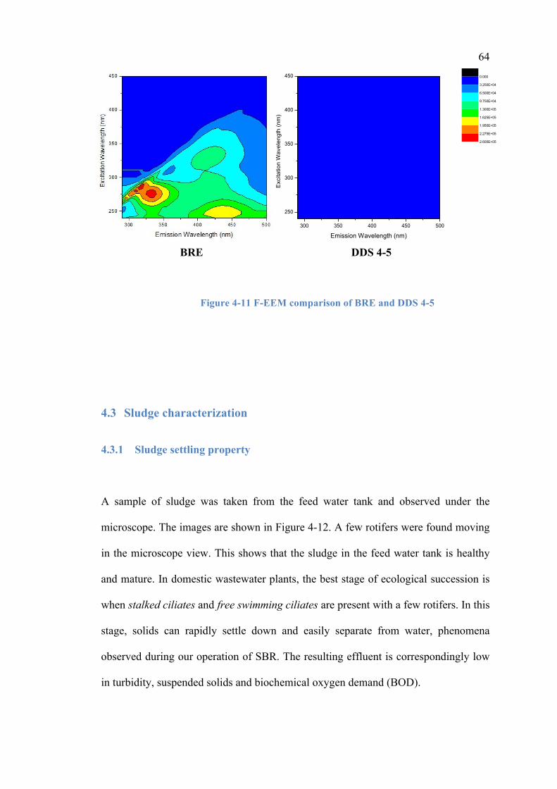
64

4.3 Sludge characterization

4.3.1 Sludge settling property

A sample of sludge was taken from the feed water tank and observed under the

microscope. The images are shown in Figure 4-12. A few rotifers were found moving

in the microscope view. This shows that the sludge in the feed water tank is healthy

and mature. In domestic wastewater plants, the best stage of ecological succession is

when stalked ciliates and free swimming ciliates are present with a few rotifers. In this

stage, solids can rapidly settle down and easily separate from water, phenomena

observed during our operation of SBR. The resulting effluent is correspondingly low

in turbidity, suspended solids and biochemical oxygen demand (BOD).

300 350 400 450 500

250

300

350

400

450

Emission Wavelength (nm)

Exc

itatio

n W

avel

engt

h (n

m)

0.000

3.250E+04

6.500E+04

9.750E+04

1.300E+05

1.625E+05

1.950E+05

2.275E+05

2.600E+05

BRE DDS 4-5

Figure 4-11 F-EEM comparison of BRE and DDS 4-5

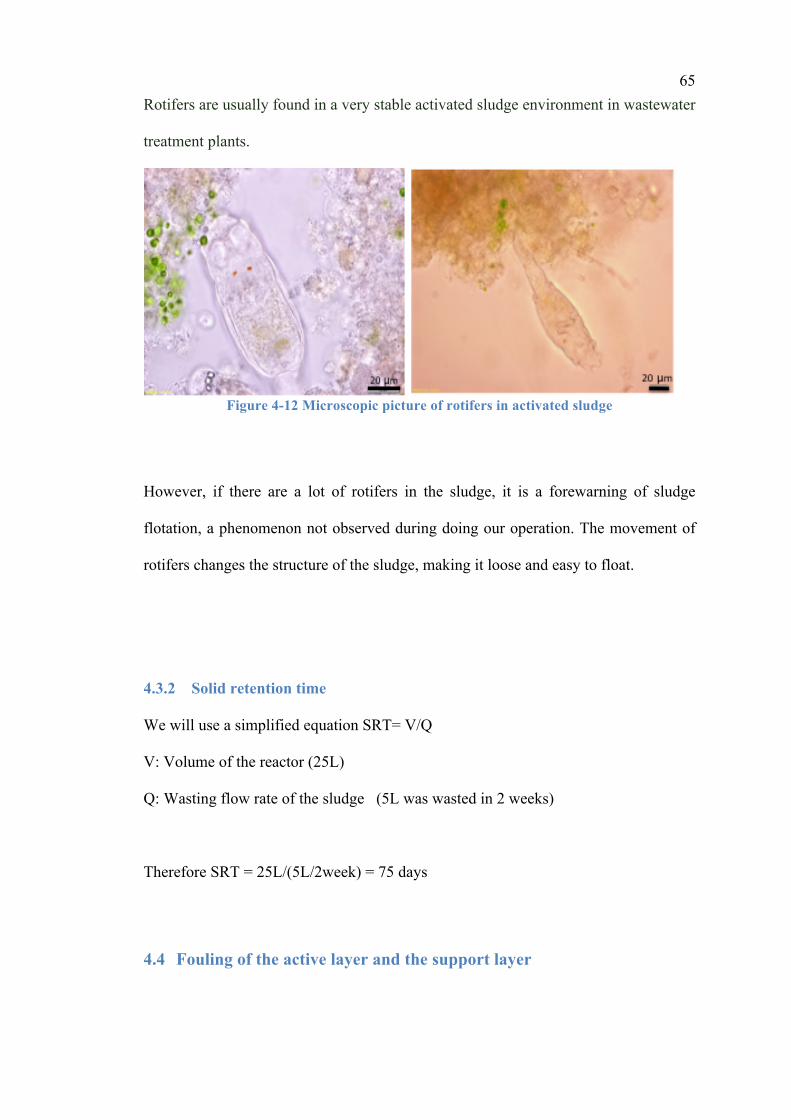
65 Rotifers are usually found in a very stable activated sludge environment in wastewater

treatment plants.

Figure 4-12 Microscopic picture of rotifers in activated sludge

However, if there are a lot of rotifers in the sludge, it is a forewarning of sludge

flotation, a phenomenon not observed during doing our operation. The movement of

rotifers changes the structure of the sludge, making it loose and easy to float.

4.3.2 Solid retention time

We will use a simplified equation SRT= V/Q

V: Volume of the reactor (25L)

Q: Wasting flow rate of the sludge (5L was wasted in 2 weeks)

Therefore SRT = 25L/(5L/2week) = 75 days

4.4 Fouling of the active layer and the support layer

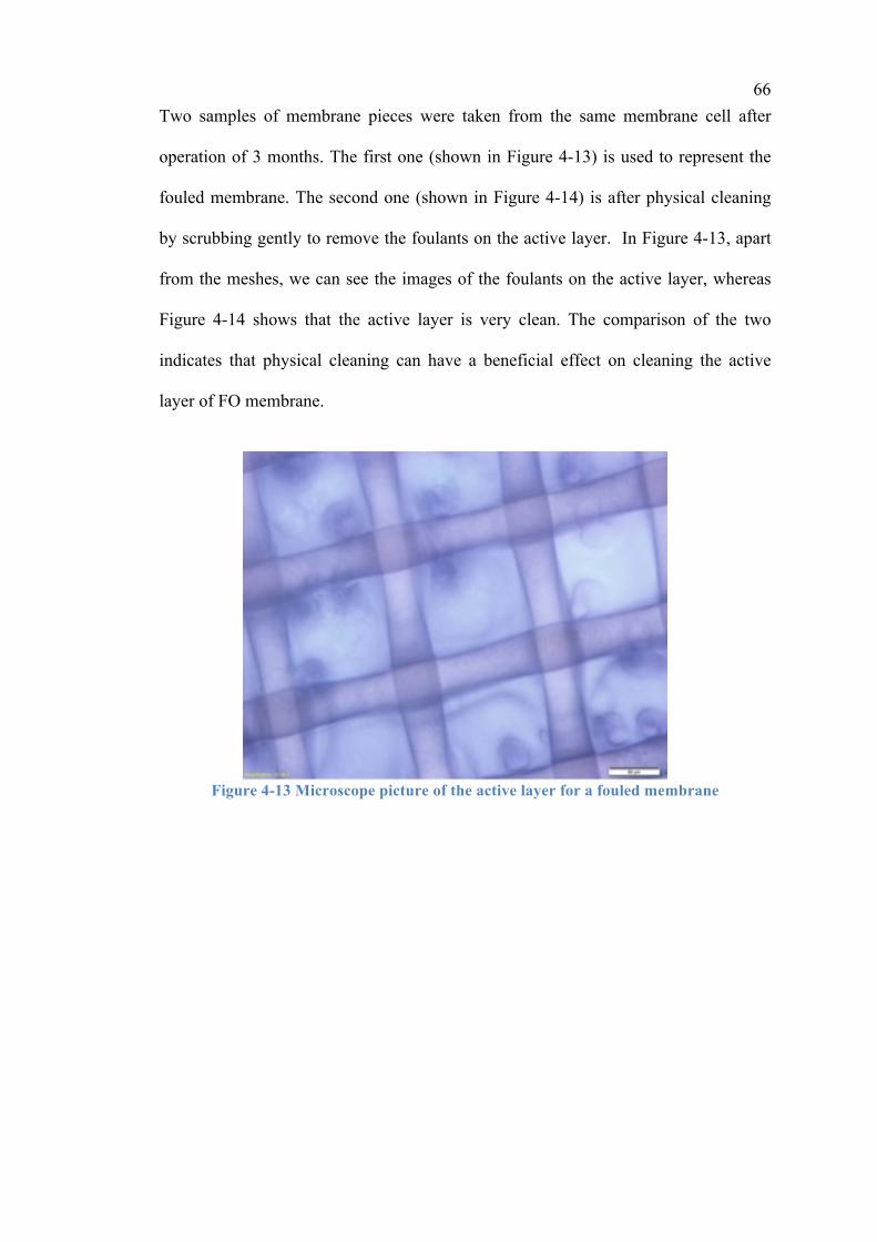
66 Two samples of membrane pieces were taken from the same membrane cell after

operation of 3 months. The first one (shown in Figure 4-13) is used to represent the

fouled membrane. The second one (shown in Figure 4-14) is after physical cleaning

by scrubbing gently to remove the foulants on the active layer. In Figure 4-13, apart

from the meshes, we can see the images of the foulants on the active layer, whereas

Figure 4-14 shows that the active layer is very clean. The comparison of the two

indicates that physical cleaning can have a beneficial effect on cleaning the active

layer of FO membrane.

Figure 4-13 Microscope picture of the active layer for a fouled membrane

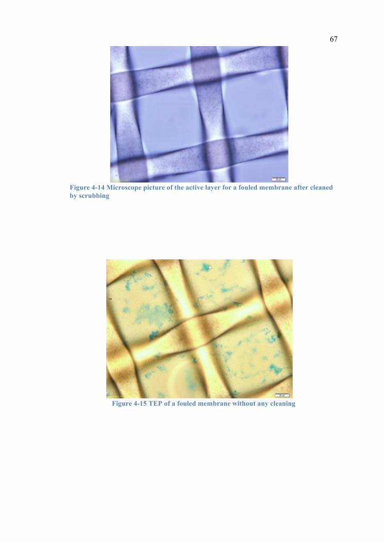
67

Figure 4-14 Microscope picture of the active layer for a fouled membrane after cleaned by scrubbing

Figure 4-15 TEP of a fouled membrane without any cleaning

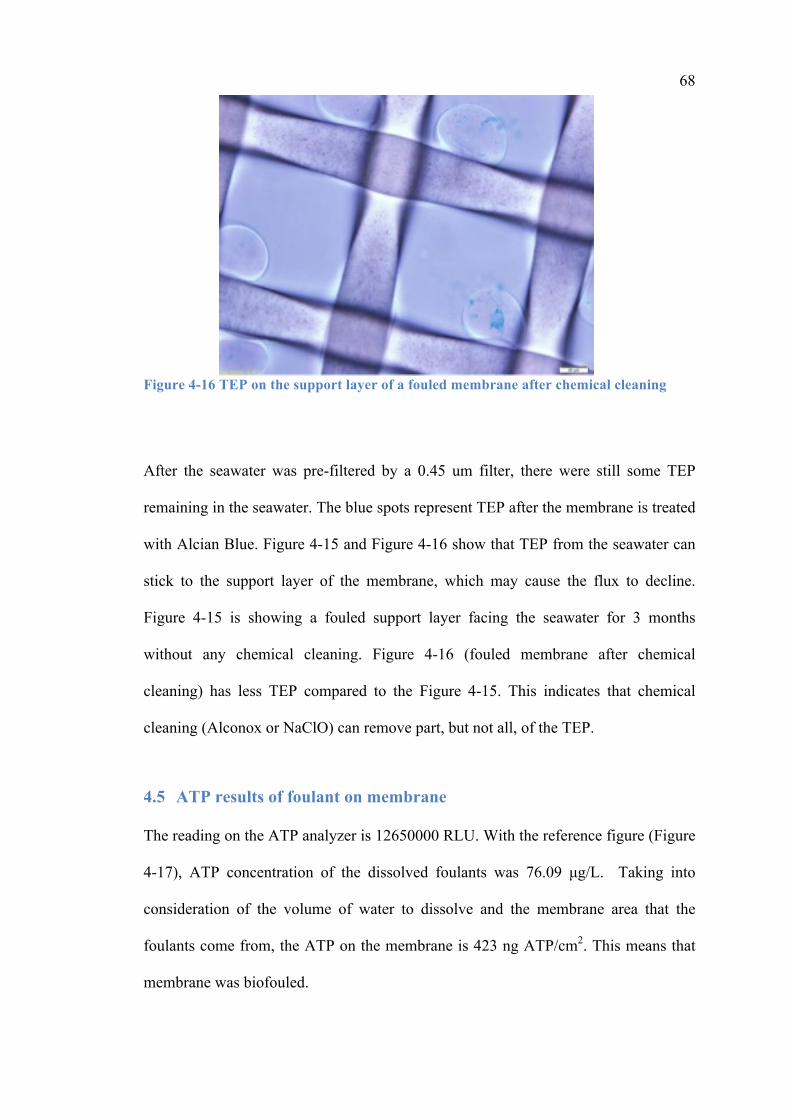
68

Figure 4-16 TEP on the support layer of a fouled membrane after chemical cleaning

After the seawater was pre-filtered by a 0.45 um filter, there were still some TEP

remaining in the seawater. The blue spots represent TEP after the membrane is treated

with Alcian Blue. Figure 4-15 and Figure 4-16 show that TEP from the seawater can

stick to the support layer of the membrane, which may cause the flux to decline.

Figure 4-15 is showing a fouled support layer facing the seawater for 3 months

without any chemical cleaning. Figure 4-16 (fouled membrane after chemical

cleaning) has less TEP compared to the Figure 4-15. This indicates that chemical

cleaning (Alconox or NaClO) can remove part, but not all, of the TEP.

4.5 ATP results of foulant on membrane

The reading on the ATP analyzer is 12650000 RLU. With the reference figure (Figure

4-17), ATP concentration of the dissolved foulants was 76.09 µg/L. Taking into

consideration of the volume of water to dissolve and the membrane area that the

foulants come from, the ATP on the membrane is 423 ng ATP/cm2. This means that

membrane was biofouled.

69

Figure 4-17 Calibration curve bewteen RLU and ATP

4.6 Chemical cleaning

4.6.1 Chemical cleaning of the active layer

The first method we used is chemical cleaning for the outside of the cell (active layer

facing the feed water). The cleaning solution was 10 g/L Alconox and 8g/L sodium

EDTA. The membrane cell was immersed in the cleaning solution 20 minutes for

each side. This cleaning method was used after 2 months of operation, when the flux

decline was 26.5%. After cleaning the active layer of the membrane with 10 g/L

Alconox and 8g/L sodium EDTA, the activated sludge attached to the membrane

surface after submerging the FO cell in the wastewater tank (shown in Figure 4-18).

70 Probably Alconox cleaning changed the surface charge of the membrane from

negative to positive. As active sludge has a negative surface potential, the sludge can

attached to the membrane easily by electrostatic interactions (Figure 4-18).

Figure 4-18 FO membrane with microbes attached after Alconox cleaning

4.6.2 Osmotic Backwash to clean the active layer

Osmotic backwash was used 20 days after the Alconox cleaning of active layer. The

membrane cell was immersed in seawater with DI water circulating inside the cell.

The effect of osmotic backwash is not clear. There is no flux recovery after the

osmotic backwash, which is also found in Qin et al., (2011). In osmotic backwash,

water is going from inside the FO cell to the outside (from the support layer to active

layer). The foulants on the active layer were washed away. But on the other hand, this

reversed flow may also push the TEP to the support layer, increasing the attachment

of TEP to the membrane. The internal concentration polarization still limits the water

flux.

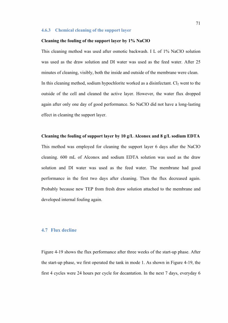
71 4.6.3 Chemical cleaning of the support layer

Cleaning the fouling of the support layer by 1% NaClO

This cleaning method was used after osmotic backwash. I L of 1% NaClO solution

was used as the draw solution and DI water was used as the feed water. After 25

minutes of cleaning, visibly, both the inside and outside of the membrane were clean.

In this cleaning method, sodium hypochlorite worked as a disinfectant. Cl2 went to the

outside of the cell and cleaned the active layer. However, the water flux dropped

again after only one day of good performance. So NaClO did not have a long-lasting

effect in cleaning the support layer.

Cleaning the fouling of support layer by 10 g/L Alconox and 8 g/L sodium EDTA

This method was employed for cleaning the support layer 6 days after the NaClO

cleaning. 600 mL of Alconox and sodium EDTA solution was used as the draw

solution and DI water was used as the feed water. The membrane had good

performance in the first two days after cleaning. Then the flux decreased again.

Probably because new TEP from fresh draw solution attached to the membrane and

developed internal fouling again.

4.7 Flux decline

Figure 4-19 shows the flux performance after three weeks of the start-up phase. After

the start-up phase, we first operated the tank in mode 1. As shown in Figure 4-19, the

first 4 cycles were 24 hours per cycle for decantation. In the next 7 days, everyday 6

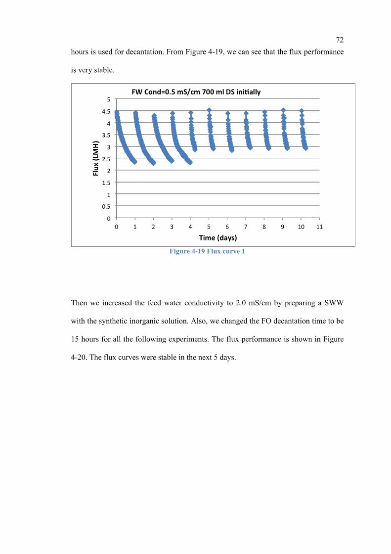
72 hours is used for decantation. From Figure 4-19, we can see that the flux performance

is very stable.

Figure 4-19 Flux curve 1

Then we increased the feed water conductivity to 2.0 mS/cm by preparing a SWW

with the synthetic inorganic solution. Also, we changed the FO decantation time to be

15 hours for all the following experiments. The flux performance is shown in Figure

4-20. The flux curves were stable in the next 5 days.

73

Figure 4-20 Flux curve 2

There were 16 days between the 16th day data of Figure 4-20 to the 17th day data of

Figure 4-21. During that period, there was microbial death due to mistaken operation.

The mistake was putting seawater directly in to the feed water tank. The microbes that

contacted the seawater could not stand the high salinity. The color of the sludge

turned to be black. We wasted 10 L of the sludge and started to increase the food for

microbes. We maintained aeration all day without FO decantation. Meanwhile, the

FO membrane cell was immersed in the tank all the time. After 16 days of restoration,

the sludge turned to a brown earthy color. TSS and VSS values were 660 mg/L and

597 mg/L respectively, back to the value before the accident.

In order to see the flux curve more efficiently, we decided to change the initial draw

solution volume to 300 mL. The flux is shown in the first curve of Figure 4-21. We

can see that the flux performance decreased considerably. This may be due to the EPS

that dead bacteria left on the membrane.

74 Why did the flux decrease considerably from day-16 to day-17?

As we changed the volume of the draw solution from 700 mL to 300 mL, the

concentration of draw solution will decrease more rapidly. Therefore, the

concentration difference between feed and draw solution become less, causing the

flux to reduce.

Therefore we were looking for methods that could recover the membrane flux. The

first method considered is to put the FO membrane cell in batch reactor effluent (BRE)

and use air scouring for 1 h trying to remove the foulants on the membrane. Then

BRE was used as feed water and the flux was shown by the green curve (the second

curve in Figure 4-21). We were not that satisfied by the performance.

So we considered to remove more foulants from the active layer of the membrane,

and chose Aloconx to clean the active layer. The detailed cleaning method was shown

in section 3.2.2.3. After Alconox cleaning, BRE was again used as feed water and the

flux was shown in the purple curve in Figure 4-21. There was no obvious change in

the performance in BRE feed.

We put the FO membrane cell back to the wastewater feed tank which had sludge

inside. As related to Figure 4-18, we observed microbes adhering to the membrane.

Then we run 4 days to see the flux performance, as shown in the light blue curves in

Figure 4-21. From this we can say Alconox cleaning did not help to restore the flux.

Even worse, it brought a new problem (biofouling) to the membrane.

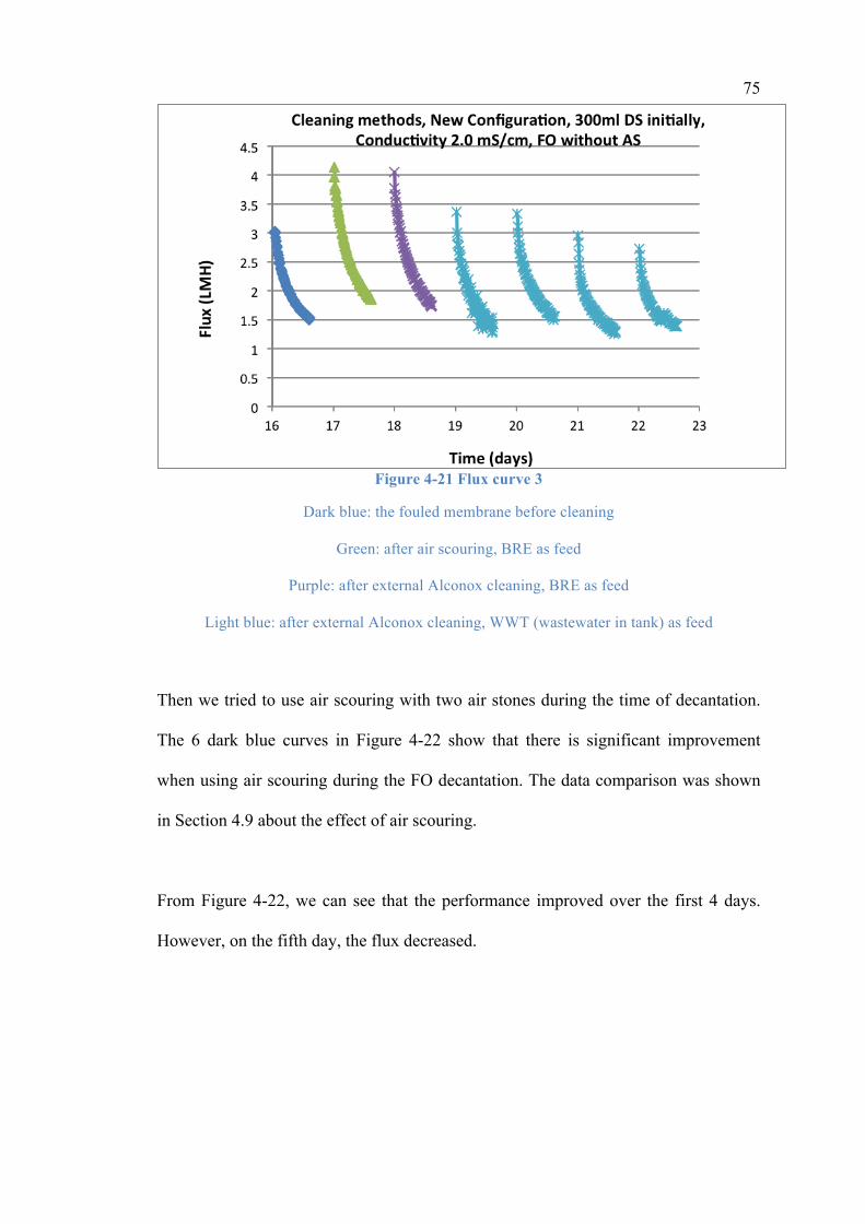
75

Figure 4-21 Flux curve 3

Dark blue: the fouled membrane before cleaning

Green: after air scouring, BRE as feed

Purple: after external Alconox cleaning, BRE as feed

Light blue: after external Alconox cleaning, WWT (wastewater in tank) as feed

Then we tried to use air scouring with two air stones during the time of decantation.

The 6 dark blue curves in Figure 4-22 show that there is significant improvement

when using air scouring during the FO decantation. The data comparison was shown

in Section 4.9 about the effect of air scouring.

From Figure 4-22, we can see that the performance improved over the first 4 days.

However, on the fifth day, the flux decreased.

76

Figure 4-22 Flux curve 4

Dark blue: FO in WWT with air scouring

Red: after osmotic backwash and internal NaClO cleaning, FO in WWT with AS

Silver: after internal Alconox cleaning, FO in WWT with AS

Before the red curves in Figure 4-22, osmotic backwash and internal NaClO cleaning

were used. However after osmotic backwash and internal NaClO cleaning, the flux

decreased. The reason might be that osmotic backwash worsened the internal TEP

fouling of the membrane and NaClO cleaning of the support layer did not have a real

effect in cleaning the internal fouling.

Therefore, we tried another cleaning method, using Alconox to clean the support layer.

The flux curves are silver in the Figure 4-22. The membrane had good performance

immediately after cleaning. Then it decreased again by the new attached TEP from

seawater and external fouling.

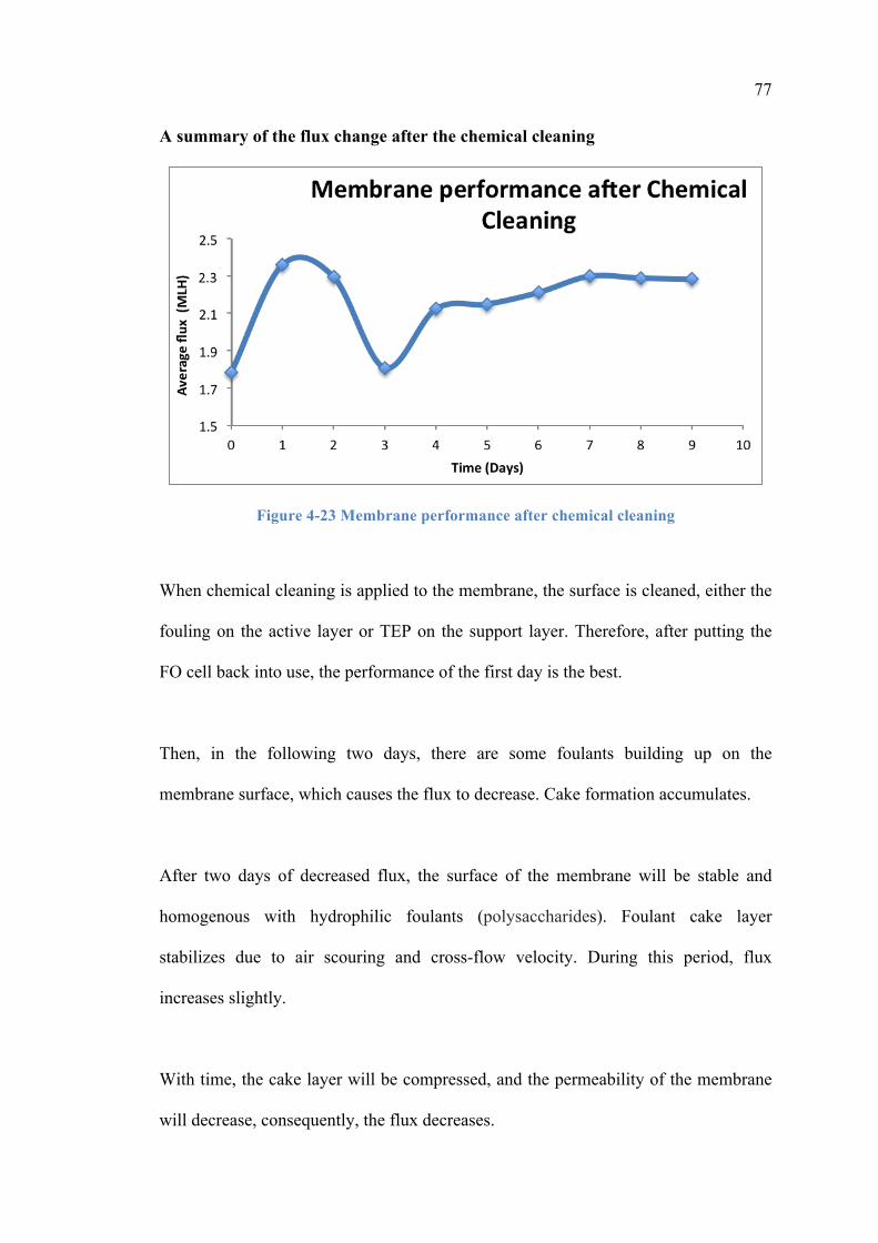
77 A summary of the flux change after the chemical cleaning

Figure 4-23 Membrane performance after chemical cleaning

When chemical cleaning is applied to the membrane, the surface is cleaned, either the

fouling on the active layer or TEP on the support layer. Therefore, after putting the

FO cell back into use, the performance of the first day is the best.

Then, in the following two days, there are some foulants building up on the

membrane surface, which causes the flux to decrease. Cake formation accumulates.

After two days of decreased flux, the surface of the membrane will be stable and

homogenous with hydrophilic foulants (polysaccharides). Foulant cake layer

stabilizes due to air scouring and cross-flow velocity. During this period, flux

increases slightly.

With time, the cake layer will be compressed, and the permeability of the membrane

will decrease, consequently, the flux decreases.

78 4.8 Water nutrients removal

4.8.1 Nutrients removal of OsSBR

When conducting experiments with Mode 2 (FO with air scouring), two water

samples were taken. One was taken from the wastewater tank immediately after

filling with food. The other was taken in the diluted draw solution after 15 hours of

FO.

For each water sample, the concentration of nitrate, nitrite, ammonium, total nitrogen

and phosphate were measured.

Table 4-6 Nutrients removal of the OsSBR process

NO3

- (mg/L)

NO2-

(mg/L) NH4

+ (mg/L)

PO43-

(mg/L) Total N (mg/L)

DDS (June 2) 16.0 0.015 1.6 0 19.6 WWT (June 1) 37.4 0.383 12.8 7.51 50.7 Removal rate 58.4% 96.2% 88.4% 100% 62.4%

DDS (Diluted draw solution)

WWT (Waste water in tank)

DDS 6-2 nitrate concentration is 16.0 mg/L, while the concentration of seawater is

less than 1 mg/L. Because the size of nitrate is small, it can pass through the

membrane and cause the nitrate level of the draw solution to increase.

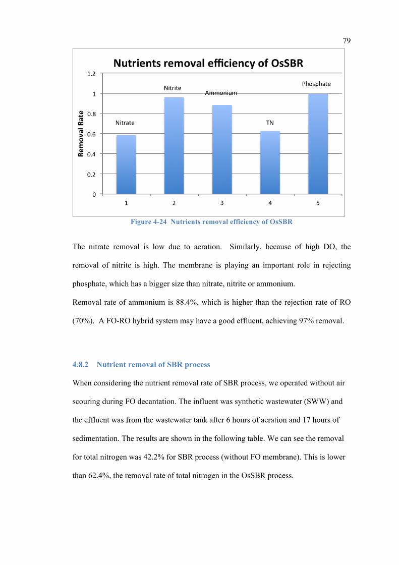
79

Figure 4-24 Nutrients removal efficiency of OsSBR

The nitrate removal is low due to aeration. Similarly, because of high DO, the

removal of nitrite is high. The membrane is playing an important role in rejecting

phosphate, which has a bigger size than nitrate, nitrite or ammonium.

Removal rate of ammonium is 88.4%, which is higher than the rejection rate of RO

(70%). A FO-RO hybrid system may have a good effluent, achieving 97% removal.

4.8.2 Nutrient removal of SBR process

When considering the nutrient removal rate of SBR process, we operated without air

scouring during FO decantation. The influent was synthetic wastewater (SWW) and

the effluent was from the wastewater tank after 6 hours of aeration and 17 hours of

sedimentation. The results are shown in the following table. We can see the removal

for total nitrogen was 42.2% for SBR process (without FO membrane). This is lower

than 62.4%, the removal rate of total nitrogen in the OsSBR process.

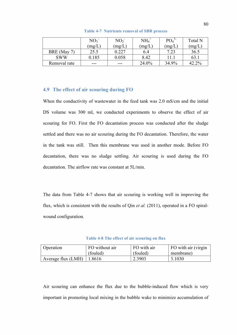
80 Table 4-7 Nutrients removal of SBR process

NO3

- (mg/L)

NO2-

(mg/L) NH4

+ (mg/L)

PO43-

(mg/L) Total N (mg/L)

BRE (May 7) 25.5 0.227 6.4 7.23 36.5 SWW 0.185 0.058 8.42 11.1 63.1

Removal rate --- --- 24.0% 34.9% 42.2%

4.9 The effect of air scouring during FO

When the conductivity of wastewater in the feed tank was 2.0 mS/cm and the initial

DS volume was 300 ml, we conducted experiments to observe the effect of air

scouring for FO. First the FO decantation process was conducted after the sludge

settled and there was no air scouring during the FO decantation. Therefore, the water

in the tank was still. Then this membrane was used in another mode. Before FO

decantation, there was no sludge settling. Air scouring is used during the FO

decantation. The airflow rate was constant at 5L/min.

The data from Table 4-7 shows that air scouring is working well in improving the

flux, which is consistent with the results of Qin et al. (2011), operated in a FO spiral-

wound configuration.

Table 4-8 The effect of air scouring on flux

Operation FO without air (fouled)

FO with air (fouled)

FO with air (virgin membrane)

Average flux (LMH) 1.8616 2.3903 3.1030

Air scouring can enhance the flux due to the bubble-induced flow which is very

important in promoting local mixing in the bubble wake to minimize accumulation of

81 solutes and molecules on the membrane (Li et al., 2006). Air scouring also helps to

remove and sweep the foulants. The cake foulant layer formed on top of the active

layer is loose. The cross flow velocity caused by air scouring can generate shear force

to break apart the foulant layer. Therefore, air scouring is effective in preventing FO

fouling. Operating FO with air scouring can reduce or eliminate the use of chemical

cleaning (Mi and Elimelech, 2010).

4.10 The effect of different orientation of the membrane

In order to see the different performances of the same FO membrane with different

orientation, we conducted the following tests.

The first orientation was active layer (AL) facing the feed water and support layer

(SL) facing the draw solution. The second orientation was active layer facing draw

solution and support layer facing feed water. The tests were done in parallel, both

with new membranes in each orientation. In Figure 4-25, the 7 flux curves on the left

were obtained in the first orientation and the 7 curves on the left were results in the

second orientation. For each orientation, the new membrane was first tested in DI

feed water for 2 days and then with BRE for 1 day, followed with 4 days of test in

wastewater tank (WWT).

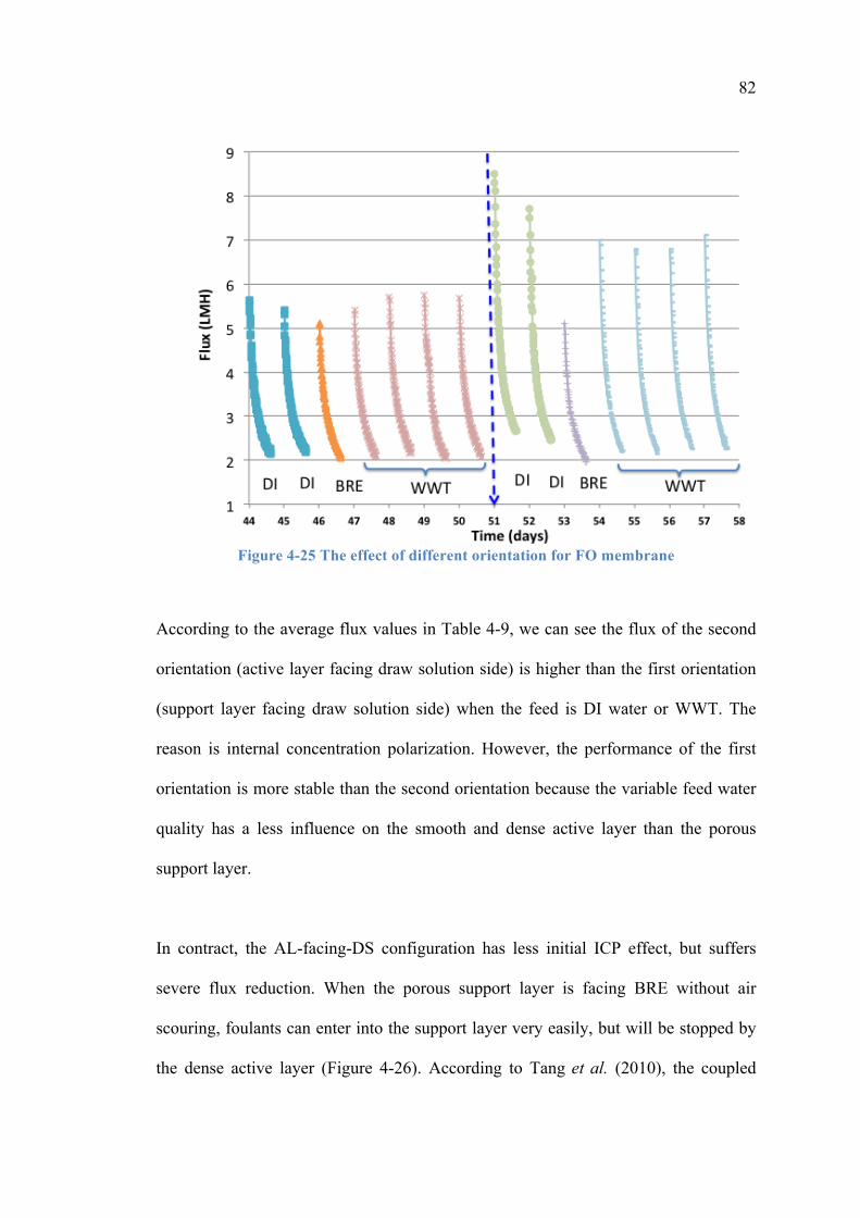
82

Figure 4-25 The effect of different orientation for FO membrane

According to the average flux values in Table 4-9, we can see the flux of the second

orientation (active layer facing draw solution side) is higher than the first orientation

(support layer facing draw solution side) when the feed is DI water or WWT. The

reason is internal concentration polarization. However, the performance of the first

orientation is more stable than the second orientation because the variable feed water

quality has a less influence on the smooth and dense active layer than the porous

support layer.

In contract, the AL-facing-DS configuration has less initial ICP effect, but suffers

severe flux reduction. When the porous support layer is facing BRE without air

scouring, foulants can enter into the support layer very easily, but will be stopped by

the dense active layer (Figure 4-26). According to Tang et al. (2010), the coupled

83 effects of internal clogging of support layer and the clogging enhanced ICP would

reduce the flux to a certain extent. This could explain why the average flux in BRE

for the AL-facing-DS orientation is lower than the AL-facing-FW orientation (shown

in Table 4-9).

Adapted from (Tang et al., 2010)

From Table 4-9, in both orientations for the new membrane, the flux in BRE (without

air scouring) is less than in WWT (with air scouring). This shows that air scouring in

WWT helps to increase the flux. Membrane surfaces are kept free of fouling by air

scouring. The result is consistent with Section 4.9.

Table 4-9 Average flux values in different feed water

Feed water First orientation (AL-facing-FW)

Second orientation (AL-facing-DS)

DI 3.0607 LMH 3.8846 LMH BRE (without air scouring) 2.9526 LMH 2.8517 LMH WWT as feed water (air) 3.1030 LMH 3.4742 LMH

Figure 4-26 A schematic illustration of ICP on membrane orientations

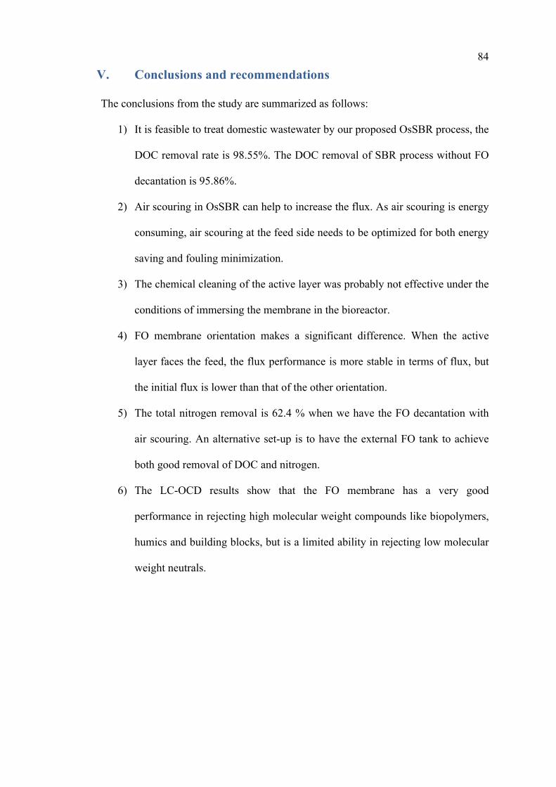
84

V. Conclusions and recommendations

The conclusions from the study are summarized as follows:

1) It is feasible to treat domestic wastewater by our proposed OsSBR process, the

DOC removal rate is 98.55%. The DOC removal of SBR process without FO

decantation is 95.86%.

2) Air scouring in OsSBR can help to increase the flux. As air scouring is energy

consuming, air scouring at the feed side needs to be optimized for both energy

saving and fouling minimization.

3) The chemical cleaning of the active layer was probably not effective under the

conditions of immersing the membrane in the bioreactor.

4) FO membrane orientation makes a significant difference. When the active

layer faces the feed, the flux performance is more stable in terms of flux, but

the initial flux is lower than that of the other orientation.

5) The total nitrogen removal is 62.4 % when we have the FO decantation with

air scouring. An alternative set-up is to have the external FO tank to achieve

both good removal of DOC and nitrogen.

6) The LC-OCD results show that the FO membrane has a very good

performance in rejecting high molecular weight compounds like biopolymers,

humics and building blocks, but is a limited ability in rejecting low molecular

weight neutrals.

85

REFERENCES

Alongi, D. M. (1998). Coastal ecosystem process. CRC press.

APHA, AWWA &WEF (2005).Standard methods for the examination of water and wastewater. Washington DC.

Atkins, P. (2006). Physical Chemistry. Oxford University Press.

Cath, T. Y., Childress, A. E. &Elimelech, M. (2006). Forward osmosis: Principles, applications, and recent developments. Journal of Membrane Science 281(1-2): 70-87.

Cath, T. Y., Hancock, N. T., Lundin, C. D., Hoppe-Jones, C. &Drewes, J. E. (2010). A multi-barrier osmotic dilution process for simultaneous desalination and purification of impaired water. Journal of Membrane Science 362(1-2): 417-426.

Chang, H. N., Moon, R. K., Park, B. G., Lim, S.-J., Choi, D. W., Lee, W. G., Song, S. L. &Ahn, Y. H. (2000). Simulation of sequential batch reactor (SBR) operation for simultaneous removal of nitrogen and phosphorus. Bioprocess and Biosystems Engineering 23(5): 513-521.

Chua, H. C., Arnot, T. C. &Howell, J. A. (2002). Controlling fouling in membrane bioreactors operated with a variable throughput. Desalination 149(1-3): 225-229.

Gray, G. T., McCutcheon, J. R. &Elimelech, M. (2006). Internal concentration polarization in forward osmosis: role of membrane orientation. Desalination 197(1-3): 1-8.

Holloway, R. W., Childress, A. E., Dennett, K. E. &Cath, T. Y. (2007). Forward osmosis for concentration of anaerobic digester centrate. Water Research 41(17): 4005-4014.

Huang, K.-J., Wei, C.-Y., Shi, Y.-M., Xie, W.-Z. &Wang, W. (2010). The investigation of the interactions between CdSe quantum dots and human serum albumin by resonance Rayleigh scattering and second-order

86 scattering spectra. Spectrochimica Acta Part A: Molecular and Biomolecular Spectroscopy 75(3): 1031-1035.

Kargi, F. &Uygur, A. (2004). Nutrient Removal in a Three-Step Sequencing Batch Reactor with Different Carbon Sources. Water, Air, &amp; Soil Pollution 156(1): 71-82.

Lay, W. C., Chong, T. H., Tang, C. Y., Fane, A. G., Zhang, J. &LIU, Y. (2010). Fouling propensity of forward osmosis: investigation of the slower flux decline phenomenon. Water Science & Technology 61(4): 927-936.

Le-Clech, P., Chen, V. &Fane, T. A. G. (2006). Fouling in membrane bioreactors used in wastewater treatment. Journal of Membrane Science 284(1-2): 17-53.

Lee, S., Boo, C., Elimelech, M. &Hong, S. (2010). Comparison of fouling behavior in forward osmosis (FO) and reverse osmosis (RO). Journal of Membrane Science 365(1-2): 34-39.

Li, Z., Youravong, W. &H-Kittikun, A. (2006). Separation of proteases from yellowfin tuna spleen by ultrafiltration. Bioresource Technology 97(18): 2364-2370.

Lim, B. R., Ahn, K. H., Song, K. G. &Cho, J. W. (2005). Microbial community in biofilm on membrane surface of submerged MBR: effect of in-line cleaning chemical agent. Water Science & Technology 51(6): 201-207.

McCutcheon, J. R., McGinnis, R. L. &Elimelech, M. (2005). A novel ammonia--carbon dioxide forward (direct) osmosis desalination process. Desalination 174(1): 1-11.

McCutcheon, J. R., McGinnis, R. L. &Elimelech, M. (2006). Desalination by ammonia-carbon dioxide forward osmosis: Influence of draw and feed solution concentrations on process performance. Journal of Membrane Science 278(1-2): 114-123.

Mi, B. &Elimelech, M. (2008). Chemical and physical aspects of organic fouling of forward osmosis membranes. Journal of Membrane Science 320(1-2): 292-302.

87 Mi, B. &Elimelech, M. (2010). Organic fouling of forward osmosis membranes:

Fouling reversibility and cleaning without chemical reagents. Journal of Membrane Science 348(1-2): 337-345.

Nopens, I., Capalozza, C. &Vanrolleghem, P. A. (2001).Stability analysis of a synthetic municipal wastewater.

Qin, J.-J., Kekre, K. A., Oo, M. H., Tao, G., Lay, C. L., Lew, C. H., Cornelissen, E. R. &Ruiken, C. J. (2011). Preliminary study of osmotic membrane bioreactor: effects of draw solution on water flux and air scouring on fouling. Water Science & Technology 62(6): 1353-1360.

Tang, C. Y., She, Q., Lay, W. C. L., Wang, R. &Fane, A. G. (2010). Coupled effects of internal concentration polarization and fouling on flux behavior of forward osmosis membranes during humic acid filtration. Journal of Membrane Science 354(1-2): 123-133.

Tchobanoglous, G., Burton, F. L. &Stensel, H. D. (2003). Wastewater engineering: treatment and reuse. NY: McGraw Hill.

Votta, F., Barnett, S. M. &Anderson, D. K. (1974).Concentration of industrial waste by direct osmosis. Providence, RI.

Vrouwenvelder, H. (2009).Biofouling of spiral wound membrane systems. Vol. PhDDelft: Delft University of Technology.

Xu, Y., Peng, X., Tang, C. Y., Fu, Q. S. &Nie, S. (2010). Effect of draw solution concentration and operating conditions on forward osmosis and pressure retarded osmosis performance in a spiral wound module. Journal of Membrane Science 348(1-2): 298-309.

Zhang, J., Chua, H. C., Zhou, J. &Fane, A. G. (2006). Factors affecting the membrane performance in submerged membrane bioreactors. Journal of Membrane Science 284(1-2): 54-66.

Zou, S., Gu, Y., Xiao, D. &Tang, C. Y. (2011). The role of physical and chemical parameters on forward osmosis membrane fouling during algae separation. Journal of Membrane Science 366(1-2): 356-362.

88

APPENDIX

Synthetic waste water recipe for 1L Urea 91.74 mg NH4Cl 12.75 mg Na-acetate 79.37 mg (Or Na-acetate. 3H2O 131.64 mg) Peptone 17.41 mg MgHPO4

. 3H2O 29.02 mg KH2PO4 23.4 mg FeSO4.7H2O 5.80 mg Starch 122.00 mg Milk Powder 116.19 mg Yeast 52.24 mg Soy oil 29.02 mg Cr(NO3)3.9H2O 0.77 mg CuCl2. 2H2O 0.536 mg MnSO4. H2O 0.108 mg NiSO4. 6H2O 0.336 mg PbCl2 0.100 mg ZnCl2 0.208 mg

Synthetic inorganic solution Chemical Weight in g (for 60L)

KCl 1.693 NH4Cl 0.009 NaCl 65.587 MgCl2.6H2O 16.416 CaCl2.6H2O 18.241 Na2CO3.H2O 0.016 NaHCO3 1.939 NaNO3 0.107 Na2SO4 0.185