1----------------------------------- · graph derivation. ... Parameterstp andqp arecomputed 8S...
150
1. Report No. VTRC 91-Rl1 4. nUe and Subtitle 2. Government A.cce•• ion No. Technical Report Documentation Page 3. Recipient's Catalog No. 5. Report Date Pressurized Storm Sewer Simulation: Model Enhancement .. -May 1991 6. Performing Organization Code 1----------------------------------- .... 8. Performing Organization "eport No. 7. Author( .) Shaw L. Yu, Yin Wu and Michelle Woodfolk 9. Performing Organization Nam. and Addr ••• Virginia Transportation Research Council P. O. Box 3817, University Station Charlottesville, Virginia 22903 12. Spon.orlng Agency Name and Addre•• Virginia Department of Transportation 1221 E. Broad Street Richmond, Virginia 23219 15. Supptementary Notes In Cooperation with the u.s. Department of Transportation Federal Highway Administration 16. Ab.tract 10. Work Unit No. (TRAIS) 11. Contract or Grant No. 2690-057-940 13. Type of Report and Period Covered FINAL REPORT July 1989 - August 1990 14. Spon.orlng A.gency Code A modified Pressurized Flow Simulation Model, PFSM, was developed and attached to the Federal Highway Administration, FHWA, Pool Funded PFP-HYDRA Package. Four hydrograph options are available for simulating inflow to a sewer system under surcharge or pressurized conditions. Several key parameters, such as time-step and print options, are dicussed on a theoretical basis for the development of guidelines recommended for parameter selection. A User's Manual for PFSII was completed, providing detailed instructions on the use of the model. 17. Key Word. Storm sewers, pressurized flow, hydraulic gradeline, microcomputer models 18. Distribution Statement No. restrictions. This document is avail- able to the public through the National Information Services, Springfield, Va. 22161 19. Security Claslf. (of this report) Unclassified Form DOT F 1700.7 (8-72) 20. Security Cla•• If. (01 this page) Unclassified Reproduction of completed page 21. No. of Page. 22. Price
Transcript of 1----------------------------------- · graph derivation. ... Parameterstp andqp arecomputed 8S...

1. Report No.
VTRC 91-Rl1
4. nUe and Subtitle
2. Government A.cce••ion No.
Technical Report Documentation Page
3. Recipient's Catalog No.
5. Report Date
Pressurized Storm Sewer Simulation: Model Enhancement.. ~~.--.- -May 1991
6. Performing Organization Code
1-----------------------------------.... 8. Performing Organization "eport No.7. Author( .)
Shaw L. Yu, Yin Wu and Michelle Woodfolk
9. Performing Organization Nam. and Addr•••
Virginia Transportation Research CouncilP. O. Box 3817, University StationCharlottesville, Virginia 22903
12. Spon.orlng Agency Name and Addre••
Virginia Department of Transportation1221 E. Broad StreetRichmond, Virginia 23219
15. Supptementary Notes
In Cooperation with the u.s. Department of TransportationFederal Highway Administration
16. Ab.tract
10. Work Unit No. (TRAIS)
11. Contract or Grant No.
2690-057-94013. Type of Report and Period Covered
FINAL REPORTJuly 1989 - August 1990
14. Spon.orlng A.gency Code
A modified Pressurized Flow Simulation Model, PFSM, was developed and attachedto the Federal Highway Administration, FHWA, Pool Funded PFP-HYDRA Package. Fourhydrograph options are available for simulating inflow to a sewer system undersurcharge or pressurized conditions. Several key parameters, such as time-step andprint options, are dicussed on a theoretical basis for the development of guidelinesrecommended for parameter selection. A User's Manual for PFSII was completed,providing detailed instructions on the use of the model.
17. Key Word.
Storm sewers, pressurized flow,hydraulic gradeline, microcomputermodels
18. Distribution Statement
No. restrictions. This document is avail-able to the public through the NationalInformation Services, Springfield, Va. 22161
19. Security Claslf. (of this report)
Unclassified
Form DOT F 1700.7 (8-72)
20. Security Cla••If. (01 this page)
Unclassified
Reproduction of completed page aut~rlzed
21. No. of Page. 22. Price


1.2:31
FINAL REPORT
PRESSURIZED STORM SEWER SIMULATION: MODEL ENHANCEMENT
ShawL. YuFaculty Research Scientist
YinWuGraduate Research Assistant
Michelle WoolfolkGraduate Research Assistant
(The opinions, findings, and conclusions expressed in thisreport are those of the authors and not necessarily
those of the sponsoring agencies.)
Virginia Transportation Research Council(A Cooperative Organization Sponsored Jointly by the
Virginia Department of Transportation andthe University of Virginia)
In Cooperation with the U.S. Department of TransportationFederal Highway Administration
Charlottesville, Virginia
May 1991VTRC 91-R11

ENVIRONMENTAL RESEARCH ADVISORY COMMITTEE
R. L. HUNDLEY, Chairman, Environmental Engineer, VDOT
D. D. MCGEEHAN, Executive Secretary, Research Scientist, VTRC
A. V. BAILEY, II, Fairfax Resident Engineer, VDOT
C. F. BOLES III, State Hydraulics Engineer, VDOT
M. G. BOLT, Salem District Environmental Manager, VDOT
W. H. BUSHMAN, Edinburg Resident Engineer, VDOT
W. R. CLEMENTS, Agronomist, VDOT
E. C. COCHRAN, JR., State Location and Design Engineer, VDOT
R. C. EDWARDS, Asst. Contract Engineer, VDOT
R. L. FINK, Asst. Maintenance Engineer, VDOT
E. P. HOGE, Preservation Programs Coordinator, Department of Historic Resources
B. N. LORD, Research Environmental Engineer, Federal Highway Administration
M. F. MENEFEE, JR., Asst. Materials Division Administrator, VDOT
S. E. MURPHY, Lynchburg District Environmental Manager, VDOT
E. T. ROBB, Asst. Environmental Engineer, VDOT
W. C. SHERWOOD, Professor of Geology, James Madison University
B. W. SUMPTER, Salem District Administrator, VDOT
E. SUNDRA, Environmental Coordinator, Federal Highway Administration

ACKNOWLEDGMENTS
The research was conducted under the general supervision of Gary Allen,Director of the Virginia Transportation Research Council. Special thanks go toHarry E. Brown, Senior Research Scientist and Team Leader, for his assistance during the course of the study. The project was financed with HPR funds administeredby the Federal Highway Administration.
Calvin F. Boles III, State Hydraulics Engineer, VDOT, and his colleague,D. M. LeGrande, are gratefully acknowledged for their assistance and many suggestions and comments made throughout the duration of the project. The writers alsothank J. Sterling Jones of the FHWA and R. Kilgore ofGKY Associates, Inc., fortheir comments and assistance.
Last, but not least, the writers thank Roger Howe, Linda Evans, Linda Barsel, Randy Combs, and Arlene Fewell, all ofVTRC, for their assistance in producingthis report.
iii

I
I
I
I
I
I
I
I
I
I
I
I
I
I
I
I
I
I
I
I
I
I
I
I
I
I
I
I
I
I
I
I
I
I
I
I
I
I
I
I
I
I
I
I
I
I
I
I
I
I
I
I
I
I
I
I
I
I
I
I
I
II

ABSTRACT
A modified Pressurized Flow Simulation Model was developed and attachedto the Federal Highway Administration's Pooled Fund PFP-HYDRA program. Fourhydrograph options are available for simulating inflow to a sewer system under surcharged or pressurized conditions. Several key parameters, such as time-step andprint options, are discussed on a theoretical basis for the development of guidelinesfor parameter selection. The User's Manual was completed, providing detailed instructions on the use of the model.
v


FINAL REPORT
PRESSURIZED STORM SEWER SIMULATION: MODEL ENHANCEMENT
ShawL. YuFaculty Research Scientist
YinWuGraduate Research Assistant
Michelle WoolfolkGraduate Research Assistant
INTRODUCTION
A microcomputer program module called the Pressurized Flow SimulationModel (PFSM) was developed by modifying the EXtended TRANsport (EXTRAN)module of the Environmental Protection Agency's Storm Water Management Model(SWMM) as described in an earlier report (Yu & Wu, 1989). PFSM, which computessewer flow, velocity, gradeline elevation, etc. under either open-channel or surcharged conditions, is being attached to the PFP-HYDRA program of the FederalHighway Administration's (FHWA) Pooled Fund HYDRAIN package. PFSM canalso be run as a stand-alone program.
The previous PFSM module generates storm hydrographs by using only therational formula and assuming a triangular hydrograph. Further improvements onhydrograph options were therefore desirable, for example, a synthetic unit hydrograph method, such as the Clark method, for ungaged watersheds. Another desirable modification was the development of an "advisory module" to help the user select pertinent flow simulation parameters, printout options, ete.
The principal objective of this study was, therefore, to modify and enhancemodels developed for pressurized flow simulations and open-channel gradeline computations to suit the needs of the Virginia Department of Transportation (VDOT).Such modifications included an enhanced hydrograph procedure and a parameterselection procedure. A user's manual for PFSM was also prepared as part of the final report. The manual provides detailed instructions on the use of the model andillustrates its use with sample runs.
ENHANCED HYDROGRAPH OPTIONS
In order to estimate inflows to the sewer system better, the modified PFSMprovides four hydrograph options for computing stormwater runoff. Previously, the

10
8fI0 6W
4Cfs
2
0
I· t·1
t·1c c
time, hours
Figure 1. Rational Method Triangular Hydrograph
rational method triangular hydrograph (Figure 1) and user-supplied hydrographswere options available for estimating inflows to the system. Two additional methods, the Soil Conservation Service's (SCS) unit hydrograph method and the Clarkmethod, which are synthetic hydrograph methods, have been incorporated into thePFSM model. These two methods offer the option of generating hydrographs basedon land characteristics when storm runoff data are not available for unit hydrograph derivation.
SCS Unit Hydrograph Method
The ses unit hydrograph method was designed for watersheds up to 1,000acres (Viessman, Lewis, & Knapp, 1989). The dimensionless unit hydrograph(Figure 2) is the result of an analysis of a large number of natural unit hydrographsfrom watersheds of a wide range of sizes and geographic locations (Viessman et al.,1989). The method requires only the determination of the time to peak and thepeak discharge. Parameters tp and qp are computed 8S follows:
where
Dtp = - + tl
2
tp = time to peak (hr)D = duration of rainfall (hr)tl =lag time (hr).
2
(eq. 1)

5432o
12:j~j
1.0
0.9
0.8
0.7
0.6o~IO
~ 0.50
tl-I ~0.4
0.3
0.2
0.1
ttp
Figure 2. Dimensionless Unit Hydrograph. Source: U.S. Department ofAgriculture. Soil Conservation Service. (1986). Urban hydrology for small watersheds('Thchnical Release No. 55). Washington, DC: Author.
The peak flow for the hydrograph is computed by approximating the unit hydrograph as a triangular shape with a base time of 8/3 tp and unit area. The peak flowis determined by
484A(eq.2)
where A =watershed area (mi2)
tp =time to peak (hr)qp = peak flow (ft3/sec).
Notice that the empirical constant, 484, or K, represents the fraction of thearea under the rising limb of the hydrograph. In other words, the constant of 484represents a hydrograph with 3/8 of its area under the rising limb. The fraction isless for a flat, swampy area (K =300) and greater for a mountainous area (K = 600).
3

The unit hydrograph can be obtained using the dimensionless hydrograph ofq / qpvs. t / tp as shown in Figure 2.
The lag time, tz, is affected by land characteristics. Watershed area, slope,and a number of other factors have been used in empirical formulas for estimatingthe lag time, whereas other empirical formulas determine lag time through a relationship with the time of concentration. Equation 3 is a general ses equation thatcalculates the lag time based on characteristics of the watershed and is used in thePFP-HYDRA calculations:
where
lO.8(S + 1)0.7
tz = 1,900yo.5
tz =lag time (hr)l = length to divide (ft)Y = average watershed slope (%)S =(1,OOO/CN) -10 = potential maximum retentioneN = SCS curve number.
(eq. 3)
The representative ses curve number for the watershed area can be determined using values listed in ses Technical Release No. 55. Soil types for thewatershed can be found on ses county soil maps. In determining the characteristiclength, 1, one can take 1as the distance from the outlet to a point with the longesttravel time.
Clark Method
The Clark method relates storage to outflow using the concept of the linearreservoir, i.e., S = KQ, where S is the storage of the reservoir, Q the discharge, andK a constant. By continuity, the time rate of change of the storage is equal to thedifference between the input and output (Chow, Maidmont, & Mays, 1988). TheClark method uses a time-area histogram to route a hydrograph through the linearreservoir (Figure 3) and a storage coefficient to satisfy the needs of continuity: Thecontinuity equation is expressed as:
Inflow - Outflow =Time rate of change of storage
or
(eq.4)
After this equation is discretized, it becomes
(eq. 5)
4

6
2
3
4
5
J
acres
area
7r-------------------------,
o 2 4 6
time, hours
8 10 12
Figure 3. Time-Area Diagram
and
(eq.6)
where2at
Co =--2K+ at
and2K- at
Cl = 2K'+ at
The unit hydrograph is found by solving for Q at the end of each time interval, M. Either a Muskingum routing method or the Muskingum-Cunge method(Viessman et al., 1989) can be used to obtain values for K specific to the watershedarea. This determination requires actual inflow and outflow hydrographs. A valueofK equal to the travel time is often used when a storage coefficient has not beenpredetermined (Viessman et al., 1989). The PFSM program module assumes a value equal to the time step ifno storage coefficient is entered.
Specific-duration unit hydrographs are determined using the S-hydrographmethod when the Clark method is used to generate a unit hydrograph. The Shydrograph results from a continuous rainfall at a constant rate for an indefiniteperiod (Chow et al., 1989). Two such S-hydrographs can then be "lagged" with the
5

appropriate time length to obtain the unit hydrograph with the desired storm duration using principles of superposition.
The time-area histogram used directly determines inflow based on the incremental area and time interval. Outflows are calculated by using equation 6 withknown values of Go and C1.
Storm runoff flows calculated with any of the hydrograph options representinflows, through inlets, into the sewer system (i.e., manholes, drop inlets, etc.). Theresulting pipe flow is routed through the sewer system to the outlet.
SELECTION OF KEY PARAMETERS
In running the pressurized flow program, it is necessary for the user to specify several key parameters, such as time step, print options, etc. The following paragraphs provide some discussion on the theoretical basis for the development ofguidelines for parameter selection. Procedures for such selection processes andsample cases are described in the attached User's Manual.
Time Step
PFSM follows the theoretical background and numerical algorithms ofEXTRAN with dynamic wave simulation capability. The program. solves the full dynamic equation for gradually varied flow (one-dimensional momentum equation andcontinuity equation) using an explicit solution technique to step forward in time.The entire sewer length is considered as a single computational reach, and the dynamic wave equation is written in backward time difference between time leveln + 1 and n for the sewer. It is expressed explicitly as
(
2
)-t( )nAt· A -A h -h
Q = 1 + g IV I Q + 2f': A A + v: u,n d,n at _ A u,n d,n Atn+1 4/3 n n nUl'l n L g n L
2.21Rn
whereQ =discharge (ft3jsec)V = velocity (ft/sec)A = area (ft2)L = the entire sewer length (ft)g = gravitational acceleration (ft/sec2)
M =time step (sec)n = Manning's coefficientR = hydraulic radius (ft)h = depth of flow (ft).
6
(eq. 7)

12'4 .-~- -~ ~)
The subscript u denotes the upstream end of a sewer (i.e., entrance), and ddenotes the downstream end (i.e., exit). The bar indicates the average of values atthe entrance and exit locations. Presumably, M = An+l -An is also the average ofthe values at the sewer ends. The junction condition used is the continuity equationexpressed explicitly in terms of the depth, H, and discharge values at the time nMas
(eq.8)
Equations 7 and 8 are solved explicitly by using a modified Euler method andhalf-step and full-step calculations. Thus, PFSM, being an explicit difference formulation, solves the flows sewer by sewer by using the one-sweep explicit solutionmethod with no need for simultaneous solution of the sewers of the network (Yen,1986). As a result, the time step, tit, is most critical to the cost and stability of thePFSM run and must satisfy the following inequalities (Roesner et al., 1981):
• Pipe:
where
• Node:
At s C'AJImax1:Q
L =the entire sewer length (ft)C' =dimensionless constantD =pipe depth (in)Hmax =maximum water-surface rise (ft;)As =corresponding surface area (ft2)I:Q =net inflow to the junctions (ft3/sec).
(eq. 9)
(eq.10)
PFSM checks each pipe for possible violation of the surface wave criteria. Ifthe time step, tit (the second parameter in the PFA command), provided by the userviolates the criteria, the program will select a new M for the pressurized flow simulation to replace the value given by the user. Based on past experience withEXTRAN, a time step of 10 sec is nearly always sufficiently small to produce outflow hydrographs and state-time traces. In most applications, 15- to 30-sec timesteps are adequate. Occasionally, time steps up to 60 sec can be used.
7

Printout Option
In PFSM, three options are available to the user for the final printout. Theseoptions can be chosen by changing the value ofpr option, the fourth parameter inthe PFA command, to 0,1, or 2. Ifpr option is equal to 0, the results ofPFSM analysis will show only the summary tables for all functions and pipes in the system. Ifpr option is 1, the summary table and the time history of depths and flows for thosejunctions and pipes given by the user will be included in the output. Ifpr option is2, the summary and the time history tables in addition to the detailed, cycle-bycycle printout will appear without normal interruption of normal page breaks. Thedetailed printout gives the depth at each junction and flow in each pipe in the system at a user-specified time interval (the third parameter in the PFA command). Ajunction in surcharge is indicated by the printing of an asterisk beside its depth.Also, if surcharge iterations are occurring at the time of the intermediate printout,PFSM will print the flow differential over the iterations required. An asterisk beside a pipe flow indicates that the flow is the normal flow for the pipe. The detailedprintout ends with the printing of the continuity balance of water passing throughthe system during the simulation. Outflows from junctions not designated as outfalls are junctions that have flooded.
MODEL TESTING
Three case examples were used to test the modified PFSM program. The useof different hydrograph options is illustrated. The selection of key parameters andthe new commands used for generating hydrographs is also described.
Example 1: Rational Method
The Campostella Road (U.S. Route 460) storm sewer in the city of Norfolk,Virginia, is located off the east end of the Campostella Bridge over the ElizabethRiver and discharges into the river. This sewer system contains 16 pipes of different lengths and ground elevations. The layout of this system is shown in Figure 16in the User's Manual. A 10-year intensity-duration-frequency (IDF) curve was usedfor computing nmoff inputs to the system. A tailwater elevation of 103.5 ft (justhigher than the crown elevation) is assumed at the outfall. This example is intended for demonstrating the use of the rational method option to generate hydrographs at junctions. This option requires three commands from the original PFPHYDRA (i.e., 8WI, STO, and RAJ) and three commands in PF8M (i.e., PFA, PHJ,and PFP). In the PFA command, a time step of 10 sec, a total simulation time of 25min, a printing interval of 1 min, and a printout option of 1 were selected. Simulation was started at 0.0 hr. The time history ofwater depths at six junctions andflows for 8 pipes were desired. Since the printout option is equal to 1, the output
8

will show the summary tables of all junctions and pipes for the system and the timehistory tables.
The entire output is shown as Table 3 of the User's Manual. The output isdivided into three parts, namely, the output of the original PFP-HYDRA, theopen-channel hydraulic gradeline, and the pressurized flow results. The pressurized flow results include the following:
• an echo of input data for simulation and a listing of pipes and junctions
• the time history of depths for six junctions and the time history of flows
• the summary tables ofmaximumflows and depths for alljunctions and pipes.
As indicated in the output, if a to-sec time step violates the stability criteria,the program computes a new M of 2 sec instead.
Example 2: SCS Unit Hydrograph Method
Example 2 demonstrates the use of the ses unit hydrograph method by giving a new command called SHY for each inflow manhole. As mentioned earlier, theses unit hydrograph method is based on land characteristics. There are six parameters required by the SHY command: watershed surface area, average slope, lengthto divide, land surface characteristics, storm duration, and total storm depth. Inthe User's Manual, Figure 20 shows an eight-line sewer system. The system contains pipes of various lengths, diameters, and roughnesses, as listed in Table 1 below. Initial conditions are specified. The time step given is 10 sec, and the totalsimulation time is 70 min. The print interval is 2 min.
The program checked the ~t value (10 sec) and found it to be too large. Anew tit of 1 sec was used.
The results for this example are shown in Table 7 of the User's Manual.
Table 1. Stadium Road Data Summary
Nodes Length Diameter Manning'sUpstream Downstream (ft) (in) n Angle
7 6 90 48 .022 226 5 345 36 .012 40
15 5 75 15 .012 05 4 93 36 .012 114 3 160 36 .012 03 2 95 36 .012 612 1 36 36 .012 0
9

Example 3: Clark Method
This is a hypothetical example to show the use of the Clark method. The hypothetical system has four pipes of varying diameter and slope. A total of 218 acresis the catchment area for this system. The catchment is divided into three areasfeeding each inlet. The total simulation time is 2 1/2 hr, and the time step given is20 sec. Each inflow hydrograph is identical (i.e., time-area diagrams and storagecoefficients are identical). Pipe system data are listed in the User's Manual (Table8). The Clark method will usually be used for large areas; therefore, the usershould pay close attention to the output. Because the system pipes may be verylong, the results may not make sense. Table 10 in the User's Manual is the systemoutput.
CONCLUSIONS
1. The modified PFSM provides four hydrograph options for computing stormwater runoff at junctions in the sewer system. The rational method is used withthe original PFP-HYDRA, hydraulic gradeline computation, and pressurizedflow simulation, whereas the ses unit hydrograph method, the Clark method,and the user-supplied hydrograph option goes directly into pressurized flowanalysis. The rational method is applied for small drainage areas; the SCS unithydrograph method can be used when land characteristics, such as watershedarea and slope, are available; and the Clark method is suitable for ungagedwatersheds if one knows the time-area histogram.
2. A time step, ~t, is one critical parameter for pressurized flow simulation. ThePFSM checks each pipe 'for possible violation of the surface wave criteria andselects a new ~t if the user-supplied ~t violates the criteria.
3. Print options make it easier for the user to read the results. The summarytable provides maximum flows in pipes and maximum depths at junctions. Thetime history table of depths prints water depth changes vs. time at a particularjunction, and the time history table of flows prints flow and velocity changes vs.time at the desired pipe. The detailed printout gives the depth at each junctionand flow in each pipe in the system at a user-specified time interval.
4. With the addition of PFSM, the capability of PFP-HYDRA is significantly enhanced. PFSM can predict the location and duration of surcharge as well asflow rate, velocity, and hydraulic gradeline at selected locations in the sewersystem.
10

RECOMMENDATIONS
1. PFSM, derived from the EXTRAN module of the model SWMM, should be usedas a sewer analysis tool when there is a possibility that pipes might be surcharged. PFSM is attached to the FHWA's Pooled Fund PFP-HYDRA programbut can also be used as a stand-alone program.
2. In general, the rational method is recommended for use with a smaller drainagearea with an upper limit of 600 acres. The SCS unit hydrograph method shouldbe used for midsized areas, up to 1,000 acres. The Clark method may be usedfor midsized areas but can also be used for larger areas (greater than 1,000acres). The Clark method has a limitation on travel time; therefore, a watershed with a small time of concentration, 10 to 20 min, should not be modeledwith this method. A user hydrograph or a triangular hydrograph generated byusing the rational method would be better for this case.
11

j?48

REFERENCES
Chow, V. T.; Maidmont, L.; and Mays, L. W. (1988). Applied hydrology. New York:McGraw-Hill Book Company.
Roesner, L. A.; Shubinski, R. P.; Aldrich, J. A.; & Camp Dresser & Mckee, Inc.(1981). Storm water management model user's manual: version III, AddendumI: EXTRAN. Cincinnati, OH: U.S. Environmental Protection Agency.
U.S. Department of Agriculture. Soil Conservation Service. (1986). Urban hydrology for small watersheds (Technical Release No. 55). Washington, DC: Author.
Viessman, W., Jr.; Lewis, G. L.; and Knapp, J. W. (1989). Introduction to hydrology(3rd ed.). New York: Harper & Row.
Yen, B. C. (1986). Hydraulics of sewers. In Advances in HYDROSCIENCE, Vol.14. Orlando, FL: Academic Press, Inc., pp. 1-122.
Yu, S. L., and Wu, Y. (1989). A microcomputer model for simulating pressurizedflow in a storm sewer system (VTRC Report No. 89-R21). Charlottesville: Virginia Transportation Research Council.
13


PRESSURIZED FLOW SIMULATION MODEL
USER'S MANUAL

I
I
I
I
I
I
I
I
I
I
I
I
I
I
I
I
I
I
I
I
I
I
I
I
I
I
I
I
I
I
I
I
I
I
I
I
I
I
I
I
I
I
I
I
I
I
I
I
I
I
I
I
I
I
I
I
I
I
I
I
I
I
I
I
I
I
I
I
I
I
I
I
I
I
I
I
I
II

TABLE OF CONTENTS
IN'TRODUCTION 1
OVERVIEW OF PRESSURIZED FLOW . . . . . . . . . . . . . . . . . . . . . . . . . . . . . . 3
TEClINICAL IN'FORMATION . . . . . . . . . . . . . . . . . . . . . . . . . . . . . . . . . . . . . . 5
Storm Inflow . . . . . . . . . . . . . . . . . . . . . . . . . . . . . . . . . . . . . . . . . . . . . . . . . . 5
Option 1: Rational Method 5
Option 2: 8CB Unit Hydrograph Method . . . . . . . . . . . . . . . . . . . . . . . . 6
Option 3: Clark Method 6
Option 4: User Hydrographs 8
Hydraulics 8
Saint 'Venant Equations 8
Choosing the Time Step 9
GLOSSARY OF ADDITIONAL COMMANDS 11
EXA.MPLES 35
Example 1: Rational Method. . . . . . . . . . . . . . . . . . . . . . . . . . . . . . . . . . . . 35
Example 2: ses Unit Hydrograph Method . . . . . . . . . . . . . . . . . . . . . . . . . 62
Example 3: Clark Method 79
Example 4: User Hydrographs . . . . . . . . . . . . . . . . . . . . . . . . . . . . . . . . . . . 89
REFERENCES 101
APPENDIX A: Calculations and Troubleshooting 103
APPENDIX B: SCS Curve Number and Overland Velocity Charts 113
iii


Table 1.
Table 2.
Table 3.
Table 4.
Table 5.
Table 6.
Table 7.
Table 8.
Table 9.
Table 10.
Table 11.
LIST OF TABLES
Loss Coefficients for PNC Command .
Campostella Road Input File .
Campostella Road Output File .
Possible Surcharging Links in PFP-HYDRA Main Program .
Stadium Road Data Summary .
Stadium Road Input File .
Stadium Road Output File .
Clark Method Example Data .
Clark Method Input File .
Clark Method Output File .
Maximum Water and Crown Elevations-Clark Method
28
36
38
62
62
63
64
79
80
81
Example............................................... 89
Table 12. North Magazine Avenue Input File. . . . . . . . . . . . . . . . . . . . . . . . . . 90
Table 13. North Magazine Avenue Output File 91
Table 14. Maximum Water and Crown Elevations-North MagazineAvenue Example . . . . . . . . . . . . . . . . . . . . . . . . . . . . . . . . . . . . . . . . . 99
Appendix A
Table A1. Incorrect Output Using North Magazine Avenue Example. . . . . .. 107
Table A2. Incorrect Input Using North Magazine Avenue Example 108
Table A3. Incorrect Output Using Clark Method Example 110
Table A4. Incorrect Input Using Clark Method Example. . . . . . . . . . . . . . . . . 112
AppendixB
Table B1. Runoff Curve Numbers for Urban Areas 115
Table B2. Runoff Curve Numbers for Cultivated Agricultural Lands . . . . . .. 116
Table B3. Runoff Curve Numbers for Other Agricultural Lands . . . . . . . . . .. 117
Table B4. Runoff Coeffiecients for Rational Method . . . . . . . . . . . . . . . . . . . .. 118
v


12 "'- ,• ~J (
LIST OF FIGURES
Figure 1. Organization of Pressurized Flow Commands 4
Figure 2. Rational Method Triangular Hydrograph . . . . . . . . . . . . . . . . . . . . 5
Figure 3. Area with Isochrones 7
Figure 4. Time-Area Histogram . . . . . . . . . . . . . . . . . . . . . . . . . . . . . . . . . . . . 8
Figure 5. BEN Diagram . . . . . . . . . . . . . . . . . . . . . . . . . . . . . . . . . . . . . . . . . . 12
Figure 6. Uniform Rainfall Hyetograph 14
Figure 7. Variable Rainfall Hyetograph 14
Figure 8. Junction 10 Hydrograph 16
Figure 9. Junction 20 Hydrograph 16
Figure 10. Junction 30 Hydrograph 17
Figure 11. Junction 40 Hydrograph 17
Figure 12. Location of Initial Depth 20
Figure 13. Location of Initial Flows and Velocities. . . . . . . . . . . . . . . . . . . . . . 21
Figure 14. System Labeling for PNC Command . . . . . . . . . . . . . . . . . . . . . . . . 29
Figure 15. Time-Area Histogram . . . . . . . . . . . . . . . . . . . . . . . . . . . . . . . . . . . . 33
Figure 16. Campostella Road Layout 35
Figure 17. Hydraulic Gradeline (Head) Computation at Junction 19 . . . . . . . 60
Figure 18. Maximum Water Depth for Junction 19 61
Figure 19. Mainline Hydraulic Gradeline Results 61
Figure 20. Stadium Road Layout. . . . . . . . . . . . . . . . . . . . . . . . . . . . . . . . . . . . 76
Figure 21. Water Surface Level for Junction 5 . . . . . . . . . . . . . . . . . . . . . . . . . 77
Figure 22. Maximum Water Elevation for J~ction 5 78
Figure 23. Flow for Pipe 54 79
AppendixB
Figure B1. Average Velocities for Estimating Travel Time. . . . . . . . . . . . . . . . 119
Figure B2. Average Velocities for Estimating Travel Time for ShallowConcentrated Flow . . . . . . . . . . . . . . . .. 120
vii

12 "'-• ~) l~

INTRODUCTION
The Pressurized Flow Simulation Model (PFSM) was developed in a previousHPR study at the Virginia Transportation Research Council (Yu & Wu, 1989). Thismodule was designed to run in the analysis phase of PFP-HYDRA. The pressurizedflow module simply adds new commands to the existing PFP-HYDRA commands toallow the user the option of computing possible surcharging within a storm sewersystem.. The pressurized flow option will work only as an analysis tool, not as a design tool.
This user documentation takes the user step by step through the use of thepressurized flow commands. (This guide is intended for use in conjunction with thePFP-HYDRA User's Manual [GKY & Associates, 1986]). This will include commandorders and selection of critical parameters. AIl pressurized flow commands will beused in conjunction with existing PFP-HYDRA commands.
This manual has four main sections. The first section is an overview of pressurized flow, discussing the main options with this module. The second section is atechnical section, discussing the general theoretical basis for the pressurized flowmodule. The third section is an overview of additional commands, and the fourthsection includes several examples of pressurized flow input and output files.

12 tJ (t
OVERVIEW OF PRESSURIZED FLOW
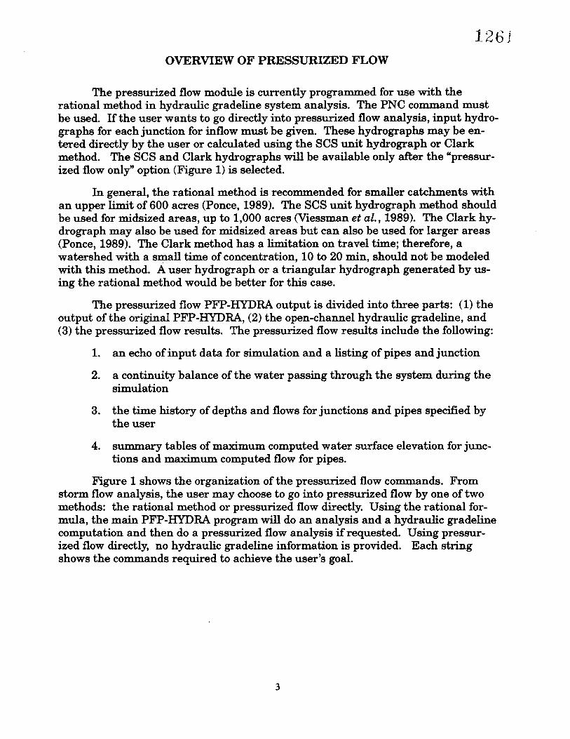
The pressurized flow module is currently programmed for use with therational method in hydraulic gradeline system analysis. The PNC command mustbe used. If the user wants to go directly into pressurized flow analysis, input hydrographs for each junction for inflow must be given. These hydrographs may be entered directly by the user or calculated using the SCS unit hydrograph or Clarkmethod. The SCS and Clark hydrographs will be available only after the "pressurized flow only" option (Figure 1) is selected.
In general, the rational method is recommended for smaller catchments withan upper limit of 600 acres (Ponce, 1989). The ses unit hydrograph method shouldbe used for midsized areas, up to 1,000 acres (Viessman et al., 1989). The Clark hydrograph may also be used for midsized areas but can also be used for larger areas(Ponce, 1989). The Clark method has a limitation on travel time; therefore, awatershed with a s~all time of concentration, 10 to 20 min, should not be modeledwith this method. A user hydrograph or a triangular hydrograph generated by using the rational method would be better for this case.
The pressurized flow PFP-HYDRA output is divided into three parts: (1) theoutput of the original PFP-HYDRA, (2) the open-channel hydraulic gradeline, and(3) the pressurized flow results. The pressurized flow results include the following:
1. an echo of input data for simulation and a listing of pipes and junction
2. a continuity balance of the water passing through the system during thesimulation
3. the time history of depths and flows for junctions and pipes specified bythe user
4. summary tables of maximum computed water surface elevation for junctions and maximum computed flow for pipes.
Figure 1 shows the organization of the pressurized flow commands. Fromstorm. flow analysis, the user may choose to go into pressurized flow by one of twomethods: the rational method or pressurized flow directly. Using the rational formula, the main PFP-HYDRA program will do an analysis and a hydraulic gradelinecomputation and then do a pressurized flow analysis if requested. Using pressurized flow directly, no hydraulic gradeline information is provided. Each stringshows the commands required to achieve the user's goal.
3

Ori
gin
al
HY
DR
Aw
ith
PN
Cco
mm
an
d
Sta
rm
Flo
wA
na
lysis
IR
ati
on
al
Me
tho
dw
ith
Pre
ssu
rize
dF
low
IP
res
su
rIz
ed
Flo
wO
nly
~ N m t"...'
•
II
Re
qu
ire
d
I
Op
tio
na
lR
eq
uir
ed
II
Op
tio
na
l
L~
Hyd
rog
rap
hl
IP
FA
Op
tio
n1
~RAI
ST
O
Pr
int
PF
AH
yd
rog
rap
hC
om
ma
nd
sO
pti
on
2
PH
JH
HJ
HH
J
tPHJ
tiDY
~
PF
PH
HD
SH
YP
FP
IQV
l.---
CH
Y
[TAD
Fig
ure
1.O
rgan
izat
ion
ofP
ress
uriz
edF
low
Com
man
ds

TECHNICAL INFORMATION
Storm Inflow
Option 1: Rational Method
Given a rainfall of constant intensity, I, uniformly distributed over a drainagearea, A, the peak discharge, Q, is given by
Q = CIA (eq. 1)
The runoff coefficient, C, represents the ratio of the nmoff volume and the rainfallvolume. Common values of C are given in Appendix B, Table B4. An inflow triangular hydrograph (Figure 2) is generated based on the flow obtained from equation1. The base of the hydrograph equals twice the time of concentration; i.e., the timeto peak equals the time of concentration (Yu & Wu, 1989).
No new commands are used to generate this hydrograph. This is automatically done when the hydraulic gradeline computation is nm simultaneously:
10
8fI0 6W
4Cfs
2
0
I· t+
t·1c c
time, hours
Figure 2. Rational Method Triangular Hydrograph
5

Option 2: SCS Unit Hydrograph Method
This hydrograph is generated using the 8eS unit hydrograph method. Thehydrograph determined using this method has a predetermined shape. However,the calculation of the hydrograph will depend heavily on the land characteristicsused. Three equations govern the formation of this hydrograph. First, the determination of the lag time is found using the following equation:
10.8(8 + 1)0.7tz = 1,900YO·5
(eq.2)
where tz =lag time (hr)1 = length to divide (ft)Y = average water course slope (%)S = potential maximum retention =(1,000/S08 curve number)
-10.
The ses curve number may be determined from the ses tables (Tables Bl throughB3, Appendix B). Composite curve numbers for an area with multiple land usecharacteristics may be calculated accordingly, as described in sas Technical Release No. 55. The length of divide is the distance from the centroid of the drainagearea to the outfall point (or point of entrance into the sewer system).
The lag time is then used to calculate the time to peak and the peak flow.All other points on the hydrograph are functions of the peak flow (SeS TechnicalRelease No. 55). The equations for these calculations are
where
and
Dtp =2" + tz
D = duration of rainfall (hr)tp = time to peak (hr)
484A
(eq. 3)
(eq.4)
where A = drainage area (sq mi)qp = peak discharge (cfs).
The HHJ and SHY commands are needed to calculate the ses hydrograph.SHY specifies the ses curve number, the drainage area (entered in acres; the program makes proper conversions), the duration of rainfall, the depth of rainfall, theland slope, and the length to divide.
Option 3: Clark Method
The calculation of the Clark hydrograph depends on the availability of atime-area diagram. The time-area diagram is a histogram of incremental area vs.
6

126~
time (Veissman et al., 1989). An area is divided into several subareas, each ofwhich has an equal travel time. The dividing lines are drawn equal time stepsapart (see Figure 3). Using a topographical map makes this determination easier.A sample time-area histogram is shown in Figure 4.
After the time-area diagram is obtained, the flow is routed using a form ofthe continuity equation:
and
where
dQI-Q =K
dt
I =inflowQ =outflowK = routing constant (user supplied)Co = f{K, time step) = 2lit/(2K + lit)C1 = 1- Co.
(eq. 5)
(eq. 6)
If a K is not specified, a default value equal to the watershed travel time is assumed. (It is recommended that the user supply K.)
Three commands are needed to calculate a Clark hydrograph. HHJ specifiesthe junctions at which hydrographs are to be calculated. TAD supplies the time-
OUTLET
Figure 3. Area with Isochrones
7

6
4
2
3
5
o
area
acres
7.-----------------------------,
o 2 4 6 8 10 12
time, hours
Figure 4. Time-Area Histogram
area diagram. CHY specifies the routing constant and the depth and duration ofthe storm.
Option 4: User Hydrographs
This option requires the user to input points defining the hydrograph. It isadvised that the user choose these points as (1) flow at 0.0 time, (2) flow at peak, (3)inflection point on recession portion, and (4) amount at the end of the storm's influence. This hydrograph may be input using two commands: HHJ and HHD. HHJspecifies the junctions at which hydrographs will be supplied, and HHD actuallycontains the hydrographs points.
Hydraulics
Saint Venant Equations
The Saint Venant equations for calculating unsteady flow are:
• Continuity:
aA aQ- +- =qat ax (eq. 7)
8

• Momentum:
1 aQ 1 a (Q2 ) ah- - + - - -- + cos8- - (So - Sf) = 0gA at gA ax A ax
(eq. 8)
The pressurized flow model uses the kinematic wave approximation of the momentum equation. This assumes that inertia terms are negligible and the friction slopeequals the bed slope (Viessman et al., 1989). The basic differential equation becomes (Yu & Wu, 1989)
aQ aA aA iJH=-gAS, + 2V- + V2- - gA-at at ax ax
Manning's equation defines the friction slope as
(eq. 9)
where
kSf = gAR4/3 Q IVI
Q = flow (ft3/sec)k = g(n/l.49)2 where n = Manning's coefficientA =cross-sectional area (ft2)R =hydraulic radius (ft)V = velocity (ft/sec)Sf = friction sloleg =32.2 ft/sec .
(eq. 10)
A finite difference numerical method is employed to calculate the flow at eachtime step, ~t.
Choosing the Time Step
Since an explicit time-varying numerical scheme is employed, a stability criterion must be established. Stability is accomplished through the use of the timestep, J1.t, which satisfies the following (Yu & Wu, 1989):
• For a conduit:
• For a node:
LAt s IgD
At s C'AJImax1:Q
9
(eq. 11)
(eq. 12)

where L = pipe length (ft)C' =0.1D = pipe depth (in)Hmcu: = maximum water surface rise (ft)As = corresponding surface area to the junction (ft2)I:Q =net inflow to the junction (cfa).
Normally, the time step will be determined using the shortest, smallest pipehaving a high inflow.
10

BEN
CHY
HHD
HHJ
IDY
IQV
NGL
PFA
PFP
PHJ
PNC*
SHY
SWI*
TAD
GLOSSARY OF ADDITIONAL COMMANDS
Allows the user to specify the bend angle and radius for a specified pipe system.
Enters a hydrograph generated by the Clark method.
Enters inflow hydrographs generated by the user.
Allows the user to specify junctions with inflow hydrographs.
Allows the user to give an initial depth.
Allows the user to give an initial velocity:
Controls the hydraulic gradeline computation.
Defines the parameters for pressurized flow analysis.
Allows the user to define pipes for a detailed printout.
Allows the user to define junctions for a detailed printout.
Defines the node-link connections for hydraulic gradeline andpressurized flow computation.
Enters a hydrograph generated by the SCS unit hydrographmethod.
Sets the switch for determining the method of storm/sanitary/pressurized flow analysis.
Allows the user to define a time-area diagram for flow.
• Commands modified from previous versions ofPFP-HYDRA.
11
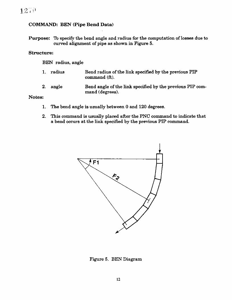
COMMAND: BEN (Pipe Bend Data)
Purpose: To specify the bend angle and radius for the computation of losses due tocurved alignment of pipe as shown in Figure 5.
Structure:
BEN radius, angle
1. radius
2. angle
Notes:
Bend radius of the link specified by the previous PIPcommand (ft).
Bend angle of the link specified by the previous PIP command (degrees).
1. The bend angle is usually between 0 and 120 degrees.
2. This command is usually placed after the PNC command to indicate thata bend occurs at the link specified by the previous PIP command.
Figure 5. BEN Diagram
12

COMMAND: CHY (Clark Hydrograph)
Purpose: To calculate an inflow hydrograph using the Clark method.
Structure:
CHY K, duration, depth
1. K
2. duration
3. depth
Parameter Selection:
Routing constant or storage constant. Used to determinehow much of the runoff is actually discharged versus howmuch is stored. If no value is entered, the default valueis equal to the travel time (hr).
Storm duration (hr).
Total storm depth (in).
1. Selection ofK The best way to select a storage constant is to use a precalculated value based on runoff data. The Muskingum/Cunge methodcan be used for determination of a storage constant. When K is notknown, a general guide is to use 1 to 2 times the travel time for the isochronal areas. The default value in the program is 1 x travel time.
2. Duration and depth selection. Both categories are based on a uniformrainfall. If a uniform rainfall is assumed, such as shown in Figure 6, thetotal depth is simply:
0.5 in/hr x 2 hr =1.0 in.
If a hyetograph ,vith a nonuniform rainfall is given, as shown in Figure 7,then the total depth is
(1.0 inlhr x 1 hr) + (2.0 in/hr x 1 hr) + (0.4 inlhr x 1 hr)
+ (0.7 inlhr x 1 hr) + (2.2 inlhr'x 1 hr) + (0.1 in/hr x 1 hr)
=6.4 in
13

COMMAND: CHY (cont.)
0.8I
nten 0.6SItY
I0.4
n/hr 0.2
time J hours
Figure 6. Uniform Rainfall Hyetograph
2
Figure 7. Variable Rainfall Hyetograph
14

COMMAND: CHY (cont.)
Notes:
1. The TAD command must precede the CHY command.
2. In order to use this method, the time of concentration of the watershedarea must be greater than 10 min. If the time of concentration is lessthan 10 min, a user or triangular hydrograph is suggested.
Example:
CHY 1.2 3.0 0.7
15

COMMAND: HHD (Hydrograph Data)
Purpose: To allow the user to input an inflow hydrograph.
Structure:
HHD time, inflow, inflow, inflow, ...
1. time
2. inflow
Time at which the inflow occurs (hr).
Flow rate (cfs).
Parameter Selection:
The input for four user hydrographs ( Figures 8 through 11) is obtained inthe following manner for a 45-min pressurized flow simulation.
flow, cfs
604530
time, minutes15
oL-.- -.J- ...L.- --'- --.I
o
5
15
10
20
Figure 8. Junction 10 Hydrograph
flow. cfs
20
15
10
5
o 15 30
time, minutes45 60
Figure 9. Junction 20 Hydrograph
16

12' t7-. ~)
COMMAND: HHD (cont.)
flow. cfs35,....--------------------,
30
25
20
15
10
5
o 15 30
time. minutes
45 60
Figure 10. Junction 30 Hydrograph
604530
time. minutes15
1.0
1.2
flow. cfs1.4 ...---------------------.,
0.4
0.0 L....-. --'-- ...Io..- -----Io ---'
o
0.8
0.2
0.6
Figure 11. Junction 40 Hydrograph
Time Jctn 10 Jetn 20 Jctn 30 Jctn40(hr) Flow (efs) Flow (efs) Flow (cfs) Flow (cfs)
0.0 1 0 0 0.60.25 10 7 23 0.80.50 18 16 14 1.01.0 5 5 1 0.6
17

COMMAND: HHD (cont.)
Notes:
1. Only four points can be input for time and discharge flows.
2. The first point must be at time 0 hours.
3. The time steps must be the same for each hydrograph.
4. The HHJ command must precede the HHD command.
Examples (hydrograph points for four nodes):
HHD 0.0 1.0 0.0 0.0 0.6
HHD 0.25 10.0 7.0 23.0 0.8
HHD 0.50 18.0 16.0 14.0 1.0
HHD 0.75 13.0 11.0 7.0 0.7
18

COMMAND: HHJ (Hydrograph Junction Input)
Purpose: To specify which junctions will have inflow hydrographs and in whatordeL '
Structure:
HHJ junction number, junction number, junction number, ...
Notes:
1. The maximum number ofjunction hydrographs is defined by field 8 onthe PFA command.
2. The PFA command must precede the HHJ command.
Example:
HHJ 10 20 30 40
19
12?/

COMMAND: IDY (Initial Depth)
Purpose: To supply the initial depth in the upstream pipe from the node for pressurized flow evaluation.
Structure:
IDY depth,depth,depth, ...
1. depth Initial depth (ft) in pipe as shown in Figure 12.
Manhole
Upstream Pipe
JunctionInflow
Figure 12. Location of Initial Depth
Notes:
1. The IQV command must precede the IDY command.
2. This command is not used with the rational method.
3. The order of entry should be exactly as junctions appear in the PNC commands preceding the PFA command. For example:
• PNC 111 11 5 1 1 1 30. 0 O.
• PNC 112 1 1 12 1 1 O. 0 O.
• PNC 120 12 1 0 4 1 15. 0 O.
The IDY command would contain depths in the following order: 11 1 12O. If any depth is zero or unknown, the zero must be entered to "hold theplace" occupied by that value. Do not confuse this order with the junctionorder in the HHJ command.
4. For an example, see the IQV example.
20

COMMAND: IQV (Initial Discharge and Velocity)
Purpose: Supplies the initial discharge and velocity in the same order as the PNCcommand specified at upstream nodes and the outfall at downstreamnodes.
Structure:
IQV discharge, velocity, discharge, velocity, ...
1. discharge
2. velocity
3. discharge
Notes:
Initial discharge in most upstream pipe (cfs).
Initial velocity in most upstream pipe (fps).
1. The values should be placed in the same order as the junctions appear inthe PNC commands preceding the PFA command.
2. The location of each data set should be as illustrated in Figure 13.
MostUpstream Pipe Manhole Manhole
~Q1v1
Figure 13. Location of Initial Velocities and Flows
Example:
IQV 5.0 0.785 5.0 3.142 5.0 7.069
Il)~ 7.0 3.0 1.5
21

COMMAND: NGL (Hydraulic Gradeline Computation Control)
Purpose: To stop the computation of the hydraulic gradeline in PFP-HYDRA.When PFP-HYDRA reads this command in the input data file, thegradeline will not be computed after the design or analysis of the systemis completed. Otherwise, PFP-HYDRA will assume that the user wantsto compute the hydraulic gradeline. This command has no parametersfollowing it. NGL can be placed anywhere in the data file.
Structure:
NGL
22

COMMAND: PFA (Pressurized Flow Data)
Purpose: To define control parameters for running the pressurized flow option.
Structure:
PFA sim time, time step, interval, pr option, start time, junctions, pipes,hydrographs, iterations, tolerance, run options
1. simtime
2. time step
3. interval
4. pr option
5. start time
6. junctions
7. pipes
8. hydrographs
9. iterations
10. tolerance
11. run options
Total simulation time to run the pressurized flow (min).
Defines the incremental time used to calculate flows(sec).
Printing interval between points in history table(integer number).
Printout type. Select:
o Summary table.
1 Summary and time history tables.
2 Summary and time history tables and a detailedprintout including each cycle result.
Start time of simulation (hr).
Junctions for detailed printing of head output whenprint option is 1 or 2 (20, max).
Pipes for detailed discharge printing when print optionis 1 or 2 (20 max).
Number ofjunctions having input hydrographs.
Maximum number of times to readjust head and flow ofsurcharged junctions.
Segment of flow in surcharged area to be used as thetolerance for ending surcharge iterations.
Run pressurized flow only combined with selecting theSWI command. Select:
1 If running pressurized flow only:
o With rational method, default value.
Notes:
1. The total simulation time should be equal to or greater than the longest basetime of hydrographs in the system plus the travel time for the longest pipe.
23

COMMAND: PFA (cont.)
2. The time step is critical in terms of computing time and the stability of the program. It must be selected carefully. Equations 11 and 12 can be used to calculate a time step if the user desires. IT a time step provided by the user violatesthe preset stability limit, the program will select an appropriate time step.
3. Iterations and tolerance control the accuracy of the solution in surchargedareas. Flows and heads in these areas are recalculated until the difference between inflow and outflow is less than the tolerance limit the user selects, or until the maximum number of iterations the user specifies has been reached. Acceptable values for iterations and tolerance have been found to be 30 and 0.05,respectively.
4. The combinations of 8WI command and run options are as follows:
SWI
66Less than 6Less than 6
Option
1o1o
Result
Pressurized flow onlyElTOr, will not runPFP-HYDRA, pressurized flow onlyPFP-HYDRA, hydraulic gradeline and
pressurized flow if necessary
Examples:
SWI2 (Rational method with summary printout.)
PFA 20. 10. 0 0 O. 4 4 0 40 0.5
SWI6 (Pressurized flow only.)
PFA 10. 10. 0 0 O. 4 4 3 40 1
24

COMMAND: PFP (Printed Flow Pipe)
Purpose: To print a list of pipes for which flows and velocities are to be printed.
Structure:
PFP pipe, pipe, pipe
1. pipe Pipe number for detail printout.
Note:
1. Prints detailed output for pipes specified in this command. Can specifyup to the number of pipes entered in field 7 of the PFA command. Amaximum of 20 pipes may be specified.
Example:
PFP 1112 13
25

COMMAND: PHJ (Printed Heads Junctions)
Purpose: To print a list of individual junctions for which water depth and watersurface elevations are to be printed.
Structure:
PHJ junction, junction, ...
Note:
1. junction Junction number for detailed printout.
1. Can specify up to the number ofjunctions entered in field 6 of the PFAcommand. A maximum of 20 junctions may be specified.
Example:
PHJ 102030
26

COMMAND: PNC (Pipe Node Connection)
Purpose: To specify the connection of links and nodes for the computation of thehydraulic gradeline. Each PNC command must immediately follow thePIP command.
Structure:
PNC pipe no., us node, us type, ds node, ds type, id main, angle, id side,angle, terminal loss, tail elev, minor loss, us invert, ds invert, shaping
1. pipe no.
2. us node
3. us type
4. ds node
5. ds type
6. id main
7. angle
8. id side
Pipe number.
Number (label) of node connecting the upstream end ofthe pipe specified in field 1.
Type of node in field 2. Select:
1" Manhole.
2 Pipe junction.
3 Pump.
4 Terminal manhole.
Number (label) of node connecting the downstream end ofthe pipe specified in field 1.
Type of node in field 4. Select:
1 Manhole.
2 Pipe junction.
3 Pump.
4 Outfall point.
Identification of pipe specified by the previous PIP command and field 1 as mainline link. Select:
1 Yes.
o No.
Deflection angle of mainline link. Always less than 90degrees.
Identification of pipe specified by the previous PIP command and field 1 as sideline pipe. Select:
27

COMMAND: PNC (cont.)
1
o
Yes.
No.
9. angle Deflection angle of sideline link. Always less than 90degrees.
10. terminal loss Loss coefficient for terminal nodes. Can be manholeloss coefficient, entrance loss coefficient, etc. The default value used is 1.5 (recommended by VDOT).
11. tail elev Tailwater elevation at the point of the system's outlet.This field is optional.
- 12. minor loss
13. us invert
14. ds invert
15. shaping
Minor loss coefficient. Required only when the downstream velocity is less than the velocity within a pipe.This field is optional. Examples are given in Table 1.
Distance of pipe invert above junction invert at upstream end (ft). This field is optional.
Distance of pipe invert above junction invert at downstream end (it). This field is optional.
Identification of inlet shaping. User can specify shapingcoefficient here. If none is available, leave blank. Program will use a default value of 0.5.
Table 1. Loss Coefficients for PNC Command
Type of Entrance
Square-cornered entrance flush with wallRounded entranceInward-projecting, square-cornered entrance
K
0.5
0.04-0.2
0.8-0.9
Source: Brater, E. F., & King, H. W. (1976). Handbook ofhydraulics for thesolution ofhydraulic engineering problems (6th ed.). New York: McGraw Hill.
Note:
1. It is suggested that the user describe the system using the technique illustrated in Figure 14. Then, pipes and node locations are easily identified.
28


COMMAND: SHY (SCS Hydrograph)
Purpose: Th give PFP-HYDRA the parameters necessary to calculate the inflowhydrograph to a node using the SCS unit hydrograph method.
Structure:
SHY area, slope, length, SCS-CN, duration, depth
Watershed area (acres).
Average land slope (%).
Length to divide (ft).
ses curve number used to describe land surface characteristics (SCS Technical Release No. 55).
Storm duration (hr).
Thtal storm depth (in).
1. area
2. slope
3. length
4. SCS-CN
5. duration
6. depth
Parameter Selection:
1. Watershed area is the area of all the land that will contribute to inflow ata particular junction. Choose this area just as in the rational method ofchoosing an area for the STO command.
2. An average land slope may be obtained by calculating slopes over severaldifferent reaches (e.g., the steeper and shallower reaches) and averagingthese.
3. The curve number may be selected according to the type of developmentthat occurs in that watershed area. For example: Given lI4-acre residentiallots in Albemarle County. ses soil classification for AlbemarleCounty is Group B. This cOlTesponds to a curve number of 75.
4. Choose the total depth of excess rainfall the storm will produce. This isthe same total depth used in the CHY command.
Notes:
1. The distance from the manhole to the catchment centroid can be used forfield 3, length.
2. The HHJ command must precede the SHY command.
3. If the watershed area has several different land characteristics, a composite SCS-eN may be entered. (See Appendix B for how to calculate thecomposite curve number.)
Example:
SHY 5.0 38.1 210.0 67.0 3.0 0.7
30

COMMAND: SWI (Criteria Switch)
Purpose: To establish the method by which PFP-HYDRA is to analyze stormflows.
Structure:
SWI number
1. number A number describing the PFP-HYDRA method. Select:
1 Sanitary analysis only:
2 Storm analysis-rational method only:
3 Storm analysis-hydrographic method only:
4 Sanitary and rational analysis.
5 Sanitary and hydrographic analysis.
6 Presswized flow simulation only. Can be combinedwith the 11th parameter of the PFA command tocontrol hydraulic gradeline computation.
31

COMMAND: TAD (TIme-Area Diagram)
Purpose: To provide a time-area diagram of the catchment flow processes for thecalculation of a hydrograph.
Structure:
TAD time, area, time, area, ...
1. time
2. area
Parameter Selection:
Time at which the subarea contributes to the outflow ofthe catchment (hr).
Area that contributes to the outflow of the catchment inthe allotted time (acres).
1. Using knowledge of land surface, obtain the slope between the junction and the point of contributing area that takes the longest time toget to the junction.
2. Look up the slope and corresponding land characteristics in FiguresB1 and B2 (Appendix B) to obtain a velocity. Divide the distance tothe point in the watershed by the velocity to get the travel time.
3. Separate the area into increments based on travel times to the junction. (Note: Time increments must be equal.)
4. Plot the time-area histogram. A sample time-area histogram is given in Figure 15.
Notes:
1. The first time-area set must be 0.0, 0.0.
2. The time-area diagram is entered from the point most downstreamto the point most upstream.
3. The time must be entered in equal steps. For example:0.0 0.2 0.4 0.6.
4. The HHJ command must precede the TAD command.
5. The CHY command must follow the TAD command.
32

12' (1'• 1 J
COMMAND: TAD (cont.)
6
4
2
3
5
o
7r----------------------~
area
acres
o 2 4 6 8 10 12
time, hours
Figure 15. Time-Area Histogram
Example:
TAD 0.0 0.0 0.25 5.2 0.50 3.1 0.75 0.0
33


EXAMPLES
Example 1: Rational Method
The Campostella Road Sewer project is located in the tidewater region of Virginia. The sewer network contains 16 pipes of different lengths and elevations,with relatively flat slopes. A lO-year intensity-duration-frequency (IDF) curve inputs runoff conditions to the system, as required by the rational method. A tailwater elevation of 103.5 ft is assumed at the outfall point. A lO-sec time step andtotal simulation time of 25 min are input for pressurized flow control parameters.The resulting input and output files appear in Tables 2 and 3. Figure 16 is a diagram of the sewer system.
~I I
II II Outfall
o -Manhole
D -Drop Inlet
- Pipe
Figure 16. Campostella Road Layout
35

Table 2. Campostella Road Input File
0010 JOB CAMPOSTELLA RO, PRESSURIZED FLOW WITH RATIONAL FORMULA0020 SWI 20030 CRI 00040 PDA .013 15 3.92 2.5 2.5 .0025 720050 RAI 0 7.1 5 7.1 8 6.4 10 6 15 5.1 20 4.5 30 3.6 40 3 +0055 50 2.6 60 2.3 120 1.4 300 1.40060 NEW LATERAL: 12 TO 110070 STO 0.23 .9 100080 PIP 213 114.44 113.95 111.42 110.7 -150085 PNC 1211 12 5 11 1 2 0 1 0 1.5 0 0.2 0 0 00090 HOL 10100 NEW LATERAL: 13 TO 140110 STO .19 .9 100120 PIP 51 114.81 113.65 109 107.63 -150125 PNC 1314 13 5 14 1 2 0 1 90 1.5 0 0.2 0 0 00130 HOL 20140 NEW LATERAL: 15 TO 220145 REM LATERAL: 15 TO 170150 STO .08 .9 50160 PIP 68 116.9 113.66 112.98 109.74 -150162 PNC 1517 15 5 17 1 2 0 1 0 1.5 0 0.2 0 0 00163 REM LATERAL: 17 TO 220164 STO .21 .9 50166 PIP 119 113.66 110.5 109.74 108.23 -150168 PNC 1722 17 1 22 1 2 0 1 90 0 0 0.2 0 0 00170 HOL 30180 NEW LATERAL: 23 TO 180185 REM LATERAL: 23 TO 220190 STO .19 .9 100200 PIP 48 112.5 110.5 108.58 108 -150210 PNC 2322 23 5 22 1 2 0 1 0 1.5 0 0.2 0 0 00220 REM LATERAL: 22 TO 190270 STO .15 .9 100280 REC 30300 PIP 37 110.5 122.25 106.5 106.1 -150305 PNC 2219 22 1 19 1 2 0 1 0 0 0 0.2 0 0 00307 REM LATERAL: 19 TO 180310 STO .63 .9 100320 PIP 95 122.25 121.39 106.1 105.5 -150325 PNC 1918 19 1 18 1 2 0 1 90 0 0 0.2 0 0 00327 HOL 30329 NEW LATERAL: 26 TO 270330 REM LATERAL: 26 TO 250332 STO .44 .9 100333 PIP 55 108.09 107.89 104.17 103.97 -150334 PNC 2625 26 5 25 1 2 0 1 0 1.5 0 0.2 0 0 00335 REM LATERAL: 25 TO 270336 STO .27 .9 100337 PIP 84 107.89 105.1 103.97 102.83 -150338 PNC 2527 25 1 27 1 2 0 1 90 0 0 0.2 0 0 00339 HOL 40340 NEW TRUNK: 10 TO 140345 REM TRUNK: 10 TO 110350 STO 1.78 .9 150360 PIP 94 113.95 113.95 108.91 108.34 -180365 PNC 1011 10 5 11 1 1 90 2 0 1.5 0 0.2 0 0 10367 REM TRUNK: 11 TO 140370 STO 0.32 .9 15
36

0375 REC 10380 PIP 340 113.95 113.65 108.34 106.81 -210390 PNC 1114 11 1 14 1 1 0 2 0 0 0 0.2 0 0 10400 REM TRUNK: 14 TO 160410 STO .19 .9 100420 REC 20440 PIP 166 113.65 114.99 106.81 105.86 -210445 PNC 1416 14 1 16 1 1 0 2 0 0 0 0.2 0 0 10447 REM TRUNK 16 TO 180450 STO .26 .9 100460 PIP 223 114.99 121.39 105.86 105.23 -210465 PNC 1618 16 1 18 1 1 0 2 0 0 0 0.2 0 0 10480 REM TRUNK: 18 TO 240490 STO .74 .9 150500 REe 30520 PIP 40 121.39 117.38 105.23 104.89 -240535 PNC 1824 18 1 24 1 1 0 2 0 0 0 0.2 0 0 10537 REM TRUNK: 24 TO 270538 FLO 0.20530 PIP 338 117.38 105.1 104.89 102.02 -240540 PNC 2427 24 1 27 1 1 0 2 0 0 0 0.2 0 0 10610 REM TRUNK: 27 TO OUT0620 STO 3.41 .9 150630 REC 40650 PIP 98 105.1 105.1 101.48 100.7 -300655 PNC 2728 27 1 28 4 1 0 2 0 0 103.2 0.2 0 0 10660 PFA 25 10 1 1 0 6 8 0 30 0.050670 PHJ 19 18 16 14 10 110680 PFP 1918 1011 1114 1416 1618 1824 2427 27280690 END
37

Table 3. Campostella Road Output File
*** PFP-HYDRA (Version of Oct. 2, 1986) *** DATE 06-04-90PAGE NO 1
CAMPOSTELLA RO, PRESSURIZED FLOW WITH RATIONAL FORMULA
Commands Read From File example.hda10 JOB20 SWI 230 CRI 040 PDA .013 15 3.92 2.5 2.5 .0025 7250 RAI 0 7.1 5 7.1 8 6.4 10 6 15 5.1 20 4.5 30 3.6 40 3 +
50 2.6 60 2.3 120 1.4 300 1.4
IDF CURVE
• 71E+01** •••••••••••••••••••••••••••••••••••••••••••••••••••••••••••••••••••.•
**
.53E+01.
*
*
.35E+01. *
**
*.18E+01.
* *
• OOE+OO* •••••••••••••••••••••••••••••••••••••••••••••••••••••••••••••••••.•....00 .71 1.43 2.14 2.86 3.57 4.29 5.00
PLOT-DATA (VALUE VS.TIME)--------------------------------------------------------------------------------
.000 7.100 2.000 1.400 .000 .000 .000 .000 .000 .000
.083 7.100 5.000 1.400 .000 .000 .000 .000 .000 .000
.133 6.400 .000 .000 .000 .000 .000 .000 .000 .000
.167 6.000 .000 .000 .000 .000 .000 .000 .000 .000
.250 5.100 .000 .000 .000 .000 .000 .000 .000 .000
.333 4.500 .000 .000 .000 .000 .000 .000 .000 .000
.500 3.600 .000 .000 .000 .000 .000 .000 .000 .000
.667 3.000 .000 .000 .000 .000 .000 .000 .000 .000
.833 2.600 .000 .000 .000 -99.000 .000 .000 .000 .0001.000 2.300 .000 .000 .000 .000 .000 .000 .000 .000
60 NEW LATERAL: 12 TO 1170 STO 0.23 .9 1080 PIP 213 114.44 113.95 111.42 110.7 -15
38
DATE 06-04-90PAGE NO 2
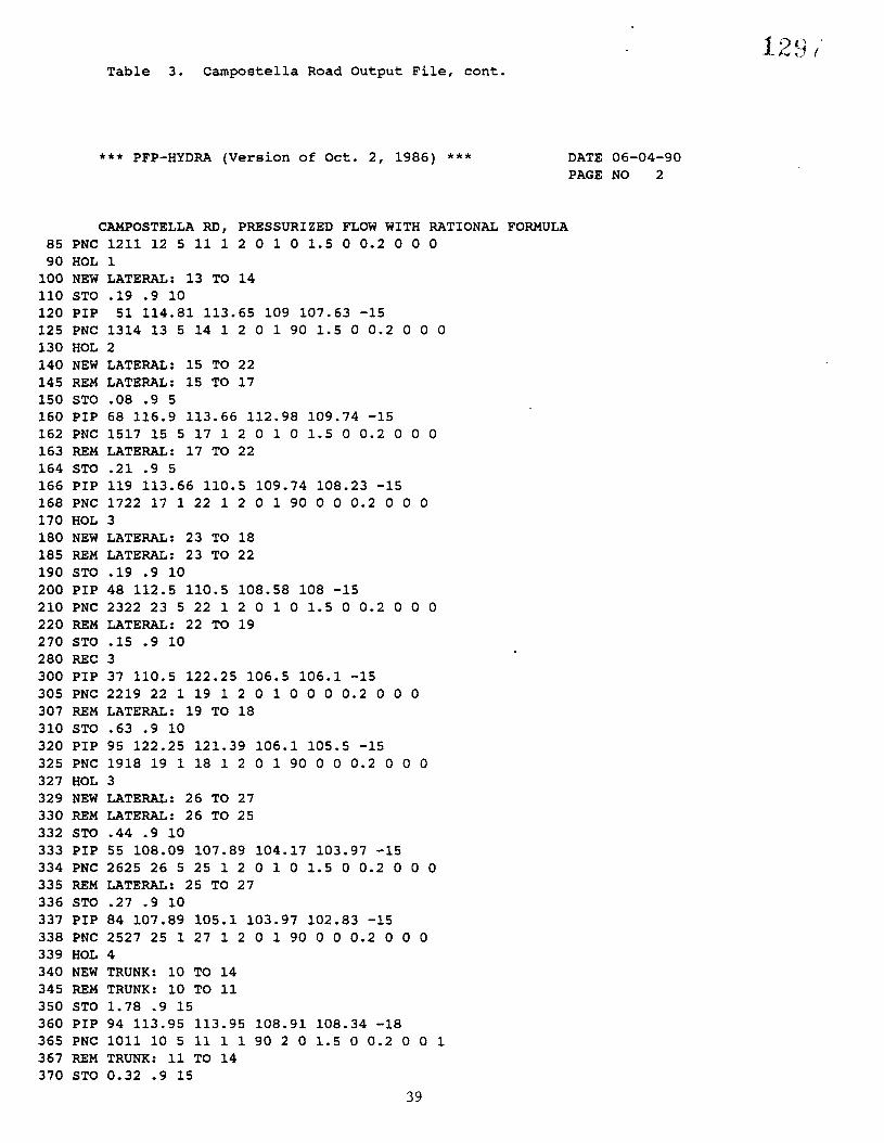
Table 3. Campostella Road Output File, cont.
*** PFP-HYDRA (Version of Oct. 2, 1986) ***
CAMPOSTELLA RD, PRESSURIZED FLOW WITH RATIONAL FORMULA85 PNC 1211 12 5 11 1 2 0 1 0 1.5 0 0.2 0 0 090 HOL 1
100 NEW LATERAL: 13 TO 14110 STO .19 .9 10120 PIP 51 114.81 113.65 109 107.63 -15125 PNC 1314 13 5 14 1 2 0 1 90 1.5 0 0.2 0 0 0130 HOL 2140 NEW LATERAL: 15 TO 22145 REM LATERAL: 15 TO 17150 STO .08 .9 5160 PIP 68 116.9 113.66 112.98 109.74 -15162 PNC 1517 15 5 17 1 2 0 1 0 1.5 0 0.2 0 0 0163 REM LATERAL: 17 TO 22164 STO .21 .9 5166 PIP 119 113.66 110.5 109.74 108.23 -15168 PNC 1722 17 1 22 1 2 0 1 90 0 0 0.2 0 0 0170 HOL 3180 NEW LATERAL: 23 TO 18185 REM LATERAL: 23 TO 22190 STO .19 .9 10200 PIP 48 112.5 110.5 108.58 108 -15210 PNC 2322 23 5 22 1 2 0 1 0 1.5 0 0.2 0 0 0220 REM LATERAL: 22 TO 19270 STO .15 .9 10280 REC 3300 PIP 37 110.5 122.25 106.5 106.1 -15305 PNC 2219 22 1 19 1 2 0 1 0 0 0 0.2 0 0 0307 REM LATERAL: 19 TO 18310 STO .63 .9 10320 PIP 95 122.25 121.39 106.1 105.5 -15325 PNC 1918 19 1 18 1 2 0 1 90 0 0 0.2 0 0 0327 HOL 3329 NEW LATERAL: 26 TO 27330 REM LATERAL: 26 TO 25332 STO .44 .9 10333 PIP 55 108.09 107.89 104.17 103.97 -15334 PNC 2625 26 5 25 1 2 0 1 0 1.5 0 0.2 0 0 0335 REM LATERAL: 25 TO 27336 STO .27 .9 10337 PIP 84 107.89 105.1 103.97 102.83 -15338 PNC 2527 25 1 27 1 2 0 1 90 0 0 0.2 0 0 0339 HOL 4340 NEW TRUNK: 10 TO 14345 REM TRUNK: 10 TO 11350 STO 1.78 .9 15360 PIP 94 113.95 113.95 108.91 108.34 -18365 PNC 1011 10 5 11 1 1 90 2 0 1.5 0 0.2 0 0 1367 REM TRUNK: 11 TO 14370 STO 0.32 .9 15
39

DATE 06-04-90PAGE NO 3
Table 3. Campostella Road Output File, cont.
*** PFP-HYDRA (Version of Oct. 2, 1986) ***
CAMPOSTELLA RO, PRESSURIZED FLOW WITH RATIONAL FORMULA375 REC 1380 PIP 340 113.95 113.65 108.34 106.81 -21390 PNC 1114 11 1 14 1 1 0 2 0 0 0 0.2 0 0 1400 REM TRUNK: 14 TO 16410 STO .19 .9 10420 REC 2440 PIP 166 113.65 114.99 106.81 105.86 -21445 PNC 1416 14 1 16 1 1 0 2 a a 0 0.2 0 0 1447 REM TRUNK 16 TO 18450 STO .26 .9 10460 PIP 223 114.99 121.39 105.86 105.23 -21465 PNC 1618 16 1 18 1 1 0 2 0 0 0 0.2 0 0 1480 REM TRUNK: 18 TO 24490 STO .74 .9 15500 REC 3520 PIP 40 121.39 117.38 105.23 104.89 -24535 PNC 1824 18 1 24 1 1 0 2 0 0 0 0.2 0 0 1537 REM TRUNK: 24 TO 27538 FLO 0.2530 PIP 338 117.38 105.1 104.89 102.02 -24540 PNC 2427 24 1 27 1 1 0 2 0 0 0 0.2 0 0 1610 REM TRUNK: 27 TO OUT620 STO 3.41 .9 15630 REC 4650 PIP 98 105.1 105.1 101.48 100.7 -30655 PNC 2728 27 1 28 4 1 0 2 0 0 103.2 0.2 0 0 1660 PFA 25 10 1 1 0 6 8 0 30 0.05670 PHJ 19 18 16 14 10 11680 PFP 1918 1011 1114 1416 1618 1824 2427 2728690 END
END OF RUN.
40

Table 3. Campostella Road Output File, cant.
*** PFP-HYDRA (Version of Oct. 2, 1986) *** DATE 06-04-90PAGE NO 4
CAMPOSTELLA RO, PRESSURIZED FLOW WITH RATIONAL FORMULA
*** LATERAL: 12 TO 11 Analysis of Existing Pipes
Link Length Diam(ft) (in)
InvertUp/Dn(ft)
Depth Cover Velocity --Flow-- -Solutions-Slope Up/Dn Up/Dn Act/Full Act/Full Load Remove Diam
(ft/ft) (ft) (ft) (ft/sec) (cfs) (%) (cfs) (in)
1 213 15 111.4 .00338110.7
3.03.3
1.71.9
2.83.1
1.243.77
33
LENGTHTOTAL LENGTH =
213.213.
COSTTOTAL COST =
o.o.
*** LATERAL: 13 TO 14 Analysis of Existing Pipes
Link Length Diam(ft) (in)
InvertUp/Dn(ft)
Depth Cover Velocity --Flow-- -Solutions-Slope Up/Dn Up/Dn Act/Full Act/Full Load Remove Diam
(ft/ft) (ft) (ft) (ft/sec) (cfs) (%) (cfs) (in)
2 51 15 109.0 .02686107.6
5.86.0
4.54.7
5.58.7
1.0310.62
10
LENGTHTOTAL LENGTH
51.51.
COST =TOTAL COST =
o.O.
*** LATERAL: 15 TO 22 Analysis of Existing Pipes
Link Length Diam(ft) (in)
InvertUp/Dn(ft)
Depth Cover Velocity --Flow-- -Solutions-Slope Up/Dn Up/Dn Act/Full Act/Full Load Remove Diam
(ft/ft) (ft) (ft) (ft/sec) (cfs) (%) (cfs) (in)
3
4
68
119
15 113.0 .04765109.7
15 109.7 .01269108.2
3.93.9
3.92.3
2.62.6
2.6.9
41
5.411.5
4.95.9
.5114.14
1.847.30
4
25

LENGTHTOTAL LENGTH
187.187.
COSTTOTAL COST
42
o.o.

Table 3. Campostella Road Output File, cont.
*** PFP-HYDRA (Version of Oct. 2, 1986) *** DATE 06-04-90PAGE NO 5
CAMPOSTELLA RD, PRESSURIZED FLOW WITH RATIONAL FORMULA
*** LATERAL: 23 TO 18 Analysis of Existing Pipes
Invert Depth Cover Velocity --Flow-- -Solutions-Link Length Diam Up/On Slope Up/On Up/on Act/Full Act/Full Load Remove Diam
(ft) (in) (ft) (ft/ft) (ft) (ft) (ft/sec) (cfs) (%) (cfs) (in)--------------------------------------------------------------------------
5 48 15 108.6 .01208 3.9 2.6 4.1 1.03 14108.0 2.5 1.1 5.8 7.12
6 37 15 106.5 .01081 4.0 2.6 5.5 3.38 50106.1 16.2 14.8 5.5 6.73
7 95 15 106.1 .00632 16.2 14.8 5.5 6.74 131 1.59 15105.5 15.9 14.5 4.2 5.15
LENGTH =TOTAL LENGTH
180.367.
COSTTOTAL COST =
o.o.
*** LATERAL: 26 TO 27 Analysis of Existing Pipes
Link Length Diam(ft) (in)
InvertUp/On(ft)
Depth Cover Velocity --Flow-- -Solutions-Slope Up/On Up/On Act/Full Act/Full Load Remove Diam
(ft/ft) (ft) (ft) (ft/sec) (cfs) (%) (cfs) (in)
8
9
55
84
15 104.2 .00364104.0
15 104.0 .01357102.8
3.93.9
3.92.3
2.62.6
2.6.9
3.33.2
6.16.1
2.383.91
3.807.55
61
50
LENGTH =TOTAL LENGTH
139.139.
COSTTOTAL COST =
43
o.o.

Table 3. Campostella Road Output File, cant.
*** PFP-HYDRA (Version of Oct. 2, 1986) *** DATE 06-04-90PAGE NO 6
CAMPOSTELLA RO, PRESSURIZED FLOW WITH RATIONAL FORMULA
*** TRUNK: 10 TO 14 Analysis of Existing Pipes
Invert Depth Cover Velocity --Flow-- -Solutions-Link Length Diam Up/On Slope Up/Dn Up/Dn Act/Full Act/Full Load Remove Diam
(ft) (in) (ft) (ft/ft) (ft) (ft) (ft/sec) (cfs) (%) (cfs) (in)--------------------------------------------------------------------------
10 94 18 108.9 .00606 5.0 3.4 5.3 8.17 100108.3 5.6 4.0 4.6 8.20
11 340 21 108.3 .00450 5.6 3.7 5.1 10.62 100106.8 6.8 4.9 4.4 10.66
12 166 21 106.8 .00572 6.8 4.9 5.0 12.02 100 .00 15105.9 9.1 7.2 5.0 12.02
13 223 21 105.9 .00283 9.1 7.2 5.4 13.00 154 4.56 18105.2 16.2 14.3 3.5 8.44
14 40 24 105.2 .00850 16.2 14.0 6.8 21.39 102 .47 15104.9 12.5 10.3 6.7 20.91
15 338 24 104.9 .00849 12.5 10.3 609 21.53 103 .63 15102.0 3.1 .9 6.7 20.90
16 98 30 101.5 .00796 3.6 .9 7.8 38.41 105 1.72 15100.7 4.4 1.7 7.5 36.69
--------------------------------------------------------------------------LENGTH = 1299. COST = O.TOTAL LENGTH = 2069. TOTAL COST = O.
44

Table 3. Campostella Road Output File, cont.
*** PFP-HYDRA (Version of Oct.2, 1986) *** DATE 06-04-90PAGE NO 7
NumberU/S D/SLink
NodeType
U/S DiSMainLine
DeflectedAngle
SideLine
SkewAngle
BendRadius Angle
[Ft]
1 12 11 5 1 2 .0 1 .0 .00 .0
2 13 14 5 1 2 .0 1 90.0 .00 .0
3 lS 17 5 1 2 .0 1 .0 .00 .0
4 17 22 1 1 2 .0 1 90.0 .00 .0
5 23 22 5 1 2 .0 1 .0 .00 .0
6 22 19 1 1 2 .0 1 .0 .00 .0
7 19 18 1 1 2 .0 1 90.0 .00 .0
8 26 25 5 1 2 .0 1 .0 .00 .0
9 25 27 1 1 2 .0 1 90.0 .00 .0
10 10 11 5 1 1 90.0 2 .0 .00 .0
11 11 14 1 1 1 .0 2 .0 .00 .0
12 14 16 1 1 1 .0 2 .0 .00 .0
13 16 18 1 1 1 .0 2 .0 .00 .0
14 18 24 1 1 1 .0 2 .0 .00 .0
15 24 27 1 1 1 .0 2 .0 .00 .0
16 27 28 1 4 1 .0 2 .0 .00 .0
45

Table 3. Campostella Road Output File, cont.
*** PFP-HYDRA (Version of Oct.2, 1986) *** DATE 06-04-90PAGE NO 8
Lowest Crown Elevation PossiblePotential Ground of Links Connecting Node Surcharging
Nodel Water Level Level Link# Elevation Location to the Link(Ft) (Ft) (Ft)
---------------------------------------------------------------------12 113.0 114.4 1 112.7 upstream Yes
11 112.7 114.0 10 109.8 Downstream Yes
13 111.7 114.8 2 110.3 upstream Yes
14 111.0 113.7 11 108.6 Downstream Yes
15 114.0 116.9 3 114.2 upstream No
17 110.7 113.7 3 111.0 Downstream No
22 108.2 110.5 6 107.8 Upstream Yes
23 109.6 112.5 5 109.8 Upstream No
19 109.0 122.3 6 107.3 Downstream Yes
18 108.4 121.4 7 106.8 Downstream Yes
26 105.3 108.1 8 105.4 upstream No
25 105.0 107.9 8 105.2 Downstream No
27 104.6 105.1 16 104.0 upstream Yes
10 113.9 114.0 10 110.4 upstream Yes
16 110.0 115.0 12 107.6 Downstream Yes
24 107.7 117.4 14 106.9 Downstream Yes
28 103.2 105.1 16 103.2 Downstream Yes
46
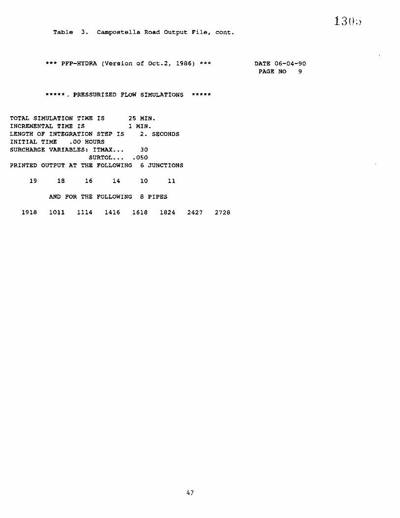
Table 3. Campostella Road Output File, cont.
*** PFP-HYDRA (Version of Oct.2, 1986) ***
***** PRESSURIZED FLOW SIMULATIONS *****
TOTAL SIMULATION TIME IS 25 MIN.INCREMENTAL TIME IS 1 MIN.LENGTH OF INTEGRATION STEP IS 2. SECONDSINITIAL TIME .00 HOURSSURCHARGE VARIABLES: ITMAX ••• 30
SURTOL ••• .050PRINTED OUTPUT AT THE FOLLOWING 6 JUNCTIONS
19 18 16 14 10 11
AND FOR THE FOLLOWING 8 PIPES
1918 1011 1114 1416 1618 1824 2427 2728
47
DATE 06-04-90PAGE NO 9

Table 3. Campostella Road Output File, cont.
*** PFP-HYDRA (Version of Oct.2, 1986) *** DATE 06-04-90PAGE NO 10
MAX.PIPE LENGTH AREA MANNING WIDTH DEPTH JUNCTIONS INVERT HEIGHT
NUMBER (FT) (SQ FT) COEF. (FT) (FT) AT ENDS ABOVE JUNCTIONS------ ------ ------- ------- --------- ---------------
1 1211 213. 1.23 .013 1.25 1.25 12 11 .00 2.362 1314 51. 1.23 .013 1.25 1.25 13 14 .00 .823 1517 68. 1.23 .013 1.25 1.25 15 17 .00 .004 1722 119. 1.23 .013 1.25 1.25 17 22 .00 1.735 2322 48. 1.23 .013 1.25 1.25 23 22 .00 1.506 2219 37. 1.23 .013 1.25 1.25 22 19 .00 .007 1918 95. 1.23 .013 1.25 1.25 19 18 .00 .278 2625 55. 1.23 .013 1.25 1.25 26 25 .00 .009 2527 84. 1.23 .013 1.25 1.25 25 27 .00 1.35
10 1011 94. 1.77 .013 1.50 1.50 10 11 .00 .0011 1114 340. 2.41 .013 1.75 1.75 11 14 .00 .0012 1416 166. 2.41 .013 1.75 1.75 14 16 .00 .0013 1618 223. 2.41 .013 1.75 1.75 16 18 .00 .0014 1824 40. 3.14 .013 2.00 2.00 18 24 .00 .0015 2427 338. 3.14 .013 2.00 2.00 24 27 .00 .,5416 2728 98. 4.91 .013 2.50 2.50 27 28 .00 .00
48

Table 3. Campostella Road Output File, cont.
*** PFP-HYDRA (Version of Oct.2, 1986) *** DATE 06-04-90PAGE NO 11
JUNCTION GROUND CROWN INVERT QINST CONNECTING PIPESNUMBER ELEV. ELEV. ELEV. (CFS)
-------- ------ ------ ----------------
1 12 114.44 112.67 111.42 .00 12112 13 114.81 110.25 109.00 .00 13143 15 116.90 114.23 112.98 .00 15174 17 113.66 110.99 109.74 .00 1517 17225 23 112.50 109.83 108.58 .00 23226 22 110.50 109.48 106.50 .00 1722 2322 22197 19 122.25 107.35 106.10 .00 2219 19188 26 108.09 105.42 104.17 .00 26259 25 107.89 105.22 103.97 .00 2625 2527
10 10 113.95 110.41 108.91 .00 101111 11 113.95 111.95 108.34 .00 1211 1011 111412 14 113.65 108.88 106.81 .00 1314 1114 141613 16 114.99 107.61 105.86 .00 1416 161814 18 121.39 107.23 105.23 .00 1918 1618 182415 24 117.38 106.89 104.89 .00 1824 242716 27 105.10 104.08 101.48 .00 2527 2427 272817 28 105.10 103.20 100.70 .00 2728
49
1 3l~ /

Table 3. Campostella Road Output File, cont.
*** PFP-HYDRA (Version of Oct.2, 1986) ***
* * * * FREE OUTFALL DATA * * * *
DATE 06-04-90PAGE NO 12
FREE OUTFLOW AT JUNCTIONS
OUTFLOW CONTROL WATER SURFACE ELEV. IS
28
103.20 FEET
* * * * SUMMARY OF INITIAL HEADS, FLOWS AND VELOCITIES * * * *
INITIAL HEADS, FLOWS AND VELOCITIES ARE ZERO
50

Table 3. Campostella Road Output File, cont.
*** PFP-HYDRA (Version of Oct.2, 1986) *** DATE 06-04-90PAGE NO 13
***** JUNCTION HYDROGRAPHS OBTAINED BY SIMPLIFIED RATIONAL FORMULA *****
JUNCTION TRIANGLE HYDROGRAPHNUMBER TIME (MIN)/INFLOW (CFS)
12 .00/ .00 10.00/ 1.24 26.70/ .0013 .00/ .00 10.00/ 1.03 26.70/ .0015 .00/ .00 5.00/ .51 13.35/ .0017 .00/ .00 5.00/ 1.34 13.35/ .0023 .00/ .00 10.00/ 1.03 26.70/ .0022 .00/ .00 10.00/ .81 26.70/ .0019 .00/ .00 10.00/ 3.40 26.70/ .0026 .00/ .00 10.00/ 2.38 26.70/ .0025 .00/ .00 10.00/ 1.46 26.70/ .0010 .00/ .00 15.00/ 8.17 40.05/ .0011 .00/ .00 15.00/ 1.47 40.05/ .0014 .00/ .00 10.00/ 1.03 26.70/ .0016 .00/ .00 10.00/ 1.40 26.70/ .0018 .00/ .00 15.00/ 3.40 40.05/ .0024 .00/ .00 .00/ .00 .00/ .0027 .00/ .00 15.00/ 15.65 40.05/ .00
51

Table 3. Campostella Road Output File, cont.
*** PFP-HYDRA (Version of Oct.2, 1986) *** DATE 06-04-90PAGE NO 14
* * * * TIME HISTORY OF HYDRAULIC GRADELINE(VALUES IN FEET)
* * * *
JUNCTION 19 JUNCTION 18 JUNCTION 16 JUNCTION 14TIME GRND 122.25 GRND 121.39 GRND 114.99 GRND 113.65
HR. MIN ELEV DEPTH ELEV DEPTH ELEV DEPTH ELEV DEPTH
o. 1 106.32 .22 105.35 .12 105.89 .03 106.84 .03o. 2 106.54 .44 105.70 .47 105.98 .12 106.95 .14o. 3 106.69 .59 105.96 .73 106.11 .25 107.13 .32o. 4 106.82 .72 106.09 .86 106.34 .48 107.31 .50o. 5 106.95 .85 106.26 1.03 106.58 .72 107.45 .64o. 6 107.06 .96 106.41 1.18 106.77 .91 107.56 .75o. 7 107.10 1.00 106.50 1.27 106.92 1.06 107.65 .84o. 8 107.17 1.07 106.57 1.34 107.07 1.21 107.73 .92o. 9 107.25 1.15 106.65 1.42 107.22 1.36 107.82 1.010.10 107.57 1.25 106.73 1.50 107.41 1.55 107.90 1.090.11 107.47 1.25 106.77 1.54 107.63 1.75 107.99 1.180.12 107.27 1.17 106.73 1.50 107.69 1.75 108.13 1.320.13 107.11 1.01 106.72 1.49 107.78 1.75 108.29 1.480.14 106.99 .89 106.70 1.47 107.86 1.75 108.51 1.700.15 106.92 .82 106.74 1.51 108.03 1.75 108.81 2.000.16 106.89 .79 106.70 1.47 107.73 1.75 108.30 1.490.17 106.80 .70 106.54 1.31 107.46 1.60 107.91 1.100.18 106.76 .66 106.56 1.33 107.66 1.75 108.09 1.280.19 106.71 .61 106.56 1.33 107.67 1.75 108.18 1.370.20 106.67 .57 106.52 1.29 107.65 1.75 108.16 1.350.21 106.62 .52 106.47 1.24 107.60 1.74 108.07 1.260.22 106.57 .47 106.43 1.20 107.53 1.67 107.95 1.140.23 106.52 .42 106.36 1.13 107.41 1.55 107.86 1.050.24 106.46 .36 106.29 1.06 107.31 1.45 107.81 1.000.25 106.40 .30 106.22 .99 107.22 1.36 107.76 .95
JUNCTION 10 JUNCTION 11TIME GRND 113.95 GRND 113.95
HR. MIN ELEV DEPTH ELEV DEPTH
o. 1 109.22 .31 108.39 .05o. 2 109.37 .46 108.61 .27o. 3 109.36 .45 108.82 .48o. 4 109.43 .52 108.94 .60o. 5 109.50 .59 109.02 .68o. 6 109.56 .65 109.08 .74o. 7 109.62 .71 109.16 .82o. 8 109.68 .77 109.24 .90o. 9 109.74 .83 109.31 .970.10 109.80 .89 109.39 1.050.11 109.86 .95 109.46 1.120.12 109.92 1.01 109.52 1.18
52

1_:31J0.13 109.98 1.07 109.58 1.240.14 110.05 1.14 109.64 1.300.15 110.14 1.23 109.80 1.460.16 111.30 1.50 108.81 .470.17 110.05 1.14 109.73 1.390.18 110.05 1.14 109.67 1.330.19 109.97 1.06 109.59 1.250.20 109.93 1.02 109.53 1.190.21 109.89 .98 109.48 1.140.22 109.86 .95 109.44 1.100.23 109.82 .91 109.40 1.060.24 109.79 .88 109.37 1.030.25 109.75 .84 109.33 .99
53
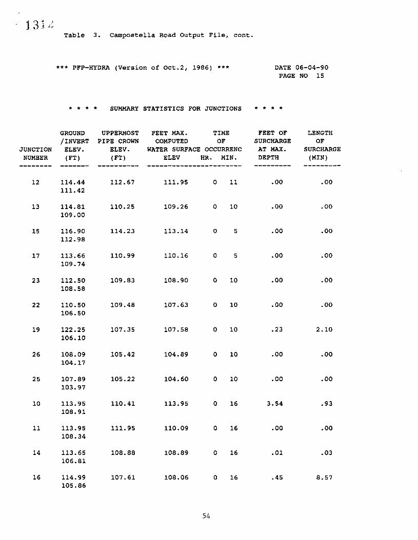
Table 3. Campostella Road Output File, cont.
*** PFP-HYDRA (Version of Oct.2, 1986) *** DATE 06-04-90PAGE NO 15
* * * * SUMMARY STATISTICS FOR JUNCTIONS * * * *
GROUND UPPERMOST FEET MAX. TIME FEET OF LENGTH/INVERT PIPE CROWN COMPUTED OF SURCHARGE OF
JUNCTION ELEV. ELEV. WATER SURFACE OCCURRENC AT MAX. SURCHARGENUMBER (FT) (FT) ELEV HR. MIN. DEPTH (MIN)
-------- ------- ---------- -------------~--------- --------- ---------12 114.44 112.67 111.95 0 11 .00 .00
111.42
13 114.81 110.25 109.26 0 10 .00 .00109.00
15 116.90 114.23 113.14 0 5 .00 .00112.98
17 113.66 110.99 110.16 0 5 .00 .00109.74
23 112.50 109.83 108.90 0 10 .00 .00108.58
22 110.50 109.48 107.63 0 10 .00 .00106.50
19 122.25 107.35 107.58 0 10 .23 2.10106.10
26 108.09 105.42 104.89 0 10 .00 .00104.17
25 107.89 105.22 104.60 0 10 .00 .00103.97
10 113.95 110.41 113.95 0 16 3.54 .93108.91
11 113.95 111.95 110.09 0 16 .00 .00108.34
14 113.65 108.88 108.89 0 16 .01 .03106.81
16 114.99 107.61 108.06 0 16 .45 8.57105.86
54

Table 3. Campostella Road Output File, cont.
*** PFP-HYDRA (Version of Oct.2, 1986) *** DATE 06-04-90PAGE NO 16
* * * * SUMMARY STATISTICS FOR JUNCTIONS * * * *
GROUND UPPERMOST FEET MAX. TIME FEET OF LENGTH/INVERT PIPE CROWN COMPUTED OF SURCHARGE OF
JUNCTION ELEV. ELEV. WATER SURFACE OCCURRENCE AT MAX. SURCHARGENUMBER (FT) (FT) ELEV HR. MIN. DEPTH (MIN)
-------- -~--~-~ ---------- ----------------------- --------- ---------
18 121.39 107.23 106.78 0 11 .00 .00105.23
24 117.38 106.89 106.38 0 15 .00 .00104.89
27 105.10 104.08 104.00 0 15 .00 .00101.48
28 105.10 103.20 103.20 0 0 .00 .00100.70
55

Table 3. Campostella Road Output File, cant.
*** PFP-HYDRA (Version of Oct.2, 1986) *** DATE 06-04-90PAGE NO 17
* * * * TIME HISTORY OF FLOW AND VELOCITYFLOW(CFS),VEL(FPS)
* * * *
TIME PIPE 1918 PIPE 1011 PIPE 1114 PIPE 1416HR. MIN FLOW VEL FLOW VEL FLOW VEL FLOW VEL
O. 1 .35 2.3 .29 2.1 .01 .7 .01 .6O. 2 1.40 3.5 1.07 3.2 .34 2.1 .14 1.7O. 3 2.36 4.1 1.57 3.4 1.29 3.1 .73 2.8O. 4 3.28 4.4 2.10 3.5 2.38 3.6 2.16 3.9O. 5 4.15 4.7 2.65 3.7 3.29 4.0 3.42 4.0O. 6 4.78 4.9 3.20 4.0 3.98 4.1 4.54 4.1O. 7 5.07 4.8 3.74 4.1 4.75 4.2 5.54 4.2O. 8 5.35 4.8 4.29 4.2 5.53 4.4 6.54 4.3O. 9 5.60 4.7 4.84 4.4 6.32 4.5 7.54 4.40.10 5.95 4.8 5.38 4.5 7.09 4.6 8.54 4.40.11 5.57 4.5 5.93 4.6 7.81 4.7 8.81 4.20.12 5.23 4.3 6.47 4.7 8.44 4.6 9.29 4.20.13 4.67 4.1 7.01 4.8 9.02 4.5 9.70 4.20.14 4.19 3.9 7.56 4.9 9.60 4.4 10.07 4.20.15 3.70 3.5 8.00 4.8 9.24 4.0 10.89 4.50.16 3.46 3.4 7.93 5.1 .11 .0 10.07 4.40.17 3.13 3.5 7.59 4.8 8.97 4.8 8.64 4.40.18 2.80 3.2 7.26 4.7 9.82 5.1 9.78 4.50.19 2.49 2.9 6.91 4.8 9.13 4.7 9.92 4.40.20 2.18 2.7 6.58 4.7 8.58 4.6 9.83 4.40.21 1.87 2.5 6.25 4.7 8.10 4.6 9.54 4.40.22 1.56 2.2 5.93 4.6 7.63 4.7 9.13 4.50.23 1.25 2.0 5.60 4.5 7.13 4.7 8.08 4.30.24 .94 1.7 5.27 4.5 6069 4.6 7.41 4.20.25 .64 1.4 4.95 4.4 6.24 4.6 6.83 4.1
TIME PIPE 1618 PIPE 1824 PIPE 2427 PIPE 2728HR. MIN FLOW VEL FLOW VEL FLOW VEL FLOW VEL
o. 1 .01 .2 .05 1.2 .00 .0 -1.91 -.9o. 2 .08 .3 .83 2.9 .07 .1 2.57 1.0o. 3 .38 .6 2.77 4.0 1.28 .8 7.84 1.4o. 4 1.35 1.5 4.98 4.8 3.78 3.2 7.40 1.9o. 5 2.93 2.4 7.54 5.5 6.45 3.6 15.10 3.2o. 6 4.44 3.0 10.11 6.0 9.18 5.3 16.88 3.9o. 7 5.71 3.4 12.05 6.4 11.40 5.8 21.15 4.7o. 8 6.88 3.7 13.70 6.6 13.13 6.3 24.16 5.3o. 9 7.99 3.9 15.34 6.9 14.76 6.6 26.93 5.90.10 9.17 4.1 17.00 7.1 16.39 6.8 29.86 6.40.11 10.17 4.4 18.42 7.3 18.04 7.0 32.44 6.80.12 10.46 4.5 18.42 7.4 18.35 6.9 33.98 7.10.13 10.85 4.6 18.51 7.4 18.50 6.8 34.93 7.2
56

1 :-3 1 -~0.14 11.13 4.7 18.49 7.5 18.48 6.7 35.65 7.3 - ~ i~)
0.15 11.87 5.0 18.90 7.5 18.72 6.6 36.41 7.40.16 11.23 4.9 18.51 7.5 18.71 6.6 36.57 7.50.17 9.41 4.4 15.90 7.2 16.48 6.4 34.79 7.30.18 10.56 4.7 16.14 7.3 15.98 6.6 32.15 6.90.19 10.59 4.7 16.04 7.2 16.09 6.7 31.33 6.70.20 10.43 4.8 15.54 7.2 15.75 6.7 30.33 6.60.21 10.11 4.7 14.75 7.1 15.01 6.7 28.80 6.30.22 9.74 4.7 13.96 7.1 14.24 6.7 27.08 6.00.23 8.90 4.5 12.80 6.9 13.23 6.5 25.23 5.70.24 8.07 4.4 11.51 6.7 11.94 6.3 22.99 5.20.25 7.37 4.3 10.35 6.5 10.75 5.9 20.77 4.8
57

Table 3. Campostella Road Output File, cont.
*** PFP-HYDRA (Version of Oct.2, 1986) *** DATE 06-04-90PAGE NO 18
* * * * SUMMARY STATISTICS FOR PIPES * * * *
PIPE MAXIMUM TIME RATIO OF MAX. DEPTH ABOVEDESIGN VERTICAL COMPUTED OF MAX. TO INVERT PIPE ENDS
PIPE FLO/VEL DEPTH FLO/VEL OCCURRENCE DESIGN UP DSNUMBER CFS/FPS (IN) CFS/FPS HR. MIN. FLOW (FT) (FT)------ ------- --------- -------- --------- -------- ----------------
1211 3.8 15.0 1.2 0 10 .3 .53 -.613.1 2.8
1314 10.6 15.0 1.0 0 10 .1 .26 1.268.6 5.4
1517 14.1 15.0 .5 0 5 .0 .16 .4211.5 2.3
1722 7.3 15.0 1.8 0 5 .2 .42 -.605.9 4.9
2322 7.1 15.0 1.0 0 10 .1 .32 -.375.8 4.1
2219 6.7 15.0 2.8 0 6 .4 1.13 1.485.5 3.8
1918 5.1 15.0 6.0 0 10 1.2 1.48 1.284.2 4.9
2625 3.9 15.0 2.4 0 10 .6 .72 .633.2 3.5
2527 7.5 15.0 3.8 0 10 .5 .63 1.176.1 5.8
1011 8.2 18.0 8.5 0 17 1.0 5.04 1.754.6 8.2
1114 10.6 21.0 9.8 0 18 .9 1.75 2.084.4 7.2
1416 12.0 21.0 10.9 0 16 .9 2.08 2.205.0 4.7
1618 8.4 21.0 11.9 0 16 1.4 2.20 1.553.5 5.1
58

Table 3. Campostella Road output File, cont.
*** PFP-HYDRA (Version of Oct.2, 1986) *** DATE 06-04-90PAGE NO 19
* * * * SUMMARY STATISTICS FOR PIPES * * * *
PIPE MAXIMUM TIME RATIO OF MAX. DEPTH ABOVEDESIGN VERTICAL COMPUTED OF MAX. TO INVERT PIPE ENDS
PIPE FLO/VEL DEPTH FLO/VEL OCCURRENCE DESIGN UP DSNUMBER CFS/FPS (IN) CFS/FPS HR. MIN. FLOW (FT) (FT)------ ------- -------- -------- ---------- -------- ----------------
1824 20.9 24.0 18.9 0 15 .9 1.55 1.496.6 7.5
2427 20.8 24.0 18.8 0 15 .9 1.49 1.986.6 7.0
2728 36.6 30.0 36.9 0 16 1.0 2.52 2.507.5 7.5
* * * * * PRESSURIZED FLOW SIMULATION ENDED * * * * *
59

Evaluation ofResults
Case 1 was run using a 10-year IDF curve to provide inflow. Notice that the10-sec time step entered in the PFA command changes during the course of the program to 2 sec. When pressurized flow checked the time step entered and found it tobe too large, the program calculated a new value.
Analyzing the various aspects of the output list (analysis, hydraulic gradeline, pressurized flow), we find a number ofjunctions at risk for surcharging. Onlyfour junctions actually surcharge in the pressurized flow analysis. A plot of the hydraulic gradeline versus time, with a value of zero at the lowest pipe invert elevation, shows where, when, and how much surcharging will occur (Figure 17). Similarplots can be constructed for other junctions to illustrate the action of the water levelin the various junctions.
Figure 18 is an illustration of the water surface elevation for Junction 19.The maximum water surface elevation is higher than the crown elevation of theuppermost link. This causes the surcharge situation. A continued evaluation of thehydraulic gradeline results shows us that the elevations from the hydraulic gradeline portion ofPFP-HYDRA are consistently higher than those of the pressurizedflow portion of PFP-HYDRA. This occurs because the hydraulic gradeline routineperforms a conservative estimate of maximum water depth. Most of the time, thehydraulic gradeline results for the mainline will follow the same trend.
Head l feetl.4 ,..--------------------------,
l,2
l,O
0,8
0.6
0.4
0.2
3025lO 15 20
Time, minutes5
0.0 '--- '--- '---__--J ---' ---''----__----'
o
Figure 17. Hydraulic Gradeline (Head) Computation at Junction 19
60

Ground Elevation 122.25'
Pipe 2219
Pipe 19181.48'
.---,.--~--------_-- Maxlmum Water Elevation107.58'
Invert EleVatl~n_106.1'
105.5' - - - - - - - - - - - - --~------------- _
Maximum Crown _Elevation 107.35'
Figure 18. Maximum Water Depth at Junction 19
140012001000600 800Oistance l ft
400200
Elevation, ft1 14 ...--------------------------~___,
110
108
1 12
102 L-.__--I ---I. --..L ----L- --'-- ---I...- _
o
106
104
- HGL Results -+- P. Flow Resul ts
Figure 19. Mainline Hydraulic Gradeline Results
61

The links in Table 4 labeled "Surcharge" are in greatest need to be sized.Other links listed are shown to be very close to the critical level. A larger stormwould cause those links to surcharge as well. (PFP-HYDRA can be used to determine the effect of placing larger diameter pipe.)
Table 4. Possible Surcharging Links in PFP-HYDRA Main Program
Junction Junction Pressurized Flow ResultsLine Upstream Downstream Ratio ofMax to Design Flow
7 19 18 1.2 Surcharge10 10 11 1.0 Surcharge11 11 14 0.912 14 16 0.913 16 18 1.4 Surcharge14 18 24 0.915 24 27 0.916 27 28 1.0 Surcharge
Example 2: SCS Unit Hydrograph Method
The Stadium Road sewer network contains eight sewers of different length,ground elevation, roughness, and diameter (see Table 5). It gives runoff parametersas required by the ses method for each inflow manhole. Initial conditions are specified. The time step given is 2 sec, and the total simulation time is 65 min. Theprint interval is 2 min. The resulting input and output files are given in Tables 6and 7. A diagram of the pipe system appears in Figure 20.
Table 5. Stadium Road Data Summary
Node Length Diameter ManningsUpstream Downstream (ft) (in) n Angle
7 6 90 48 .022 226 5 345 36 .012 40
15 5 75 15 .012 05 4 93 36 .012 114 3 160 36 .012 03 2 95 36 .012 612 1 36 36 .012 0
62

Table 6. Stadium Road Input File
0010 JOB Stadium Road Example with SCS Hydrographs0015 SWI 60035 NEW LINK 7 TO 50037 REM LINE 7-60036 FLO 5.00040 PDA .022 12 4 3 2 .0010060 PIP 90 546 525 541.9 520.9 -120070 PNC 76 7 5 6 1 1 22.0 2 0.0 1.5 0 0 0 0.1 00075 REM LINE 6-50080 PDA .014 12 4 3 2 .0010100 PIP 345 525 505 520.3 500.4 -180110 PNC 65 6 1 5 1 2 o. 1 40. 0 0 0 0 0.1 00115 NEW LINK 15 TO 10017 REM LINE 15-50130 PIP 75 510 505 505.9 500.9 -120140 PNC 155 15 5 5 1 1 O. 2 O. 0 0 0 0 0.1 00145 REM LINE 5-40160 PIP 93 505 504 500.3 499.4 -180170 PNC 54 5 1 4 1 1 11. 2 O. 0 0 0 0 0.1 00175 REM LINE 4-30190 PIP 160 504.8 504.5 498.4 498.2 -300210 PNC 43 4 1 3 2 1 O. 2 O. 0 0 0 0 0.1 00220 REM LINE 3-130230 PIP 10 504.5 504 498.2 498.1 -300240 PNC 313 3 2 13 1 1 61. 2 o. 0 0 0 0 0.1 00250 REM LINE 13-20260 PIP 85 504 502 496.5 496.3 -300270 PNC 132 13 1 2 1 2 O. 1 48. 0 0 0 0 0.1 00280 REM LINE 2-10290 PIP 25 502 500 495.1 494.8 -240300 PNC 21 2 1 1 4 1 o. 2 o. 0 0 0 0 0.1 00310 PFA 65 2. 2 1 O. 3 3 7 30 .05 10312 PHJ 5 4 20317 PFP 132 54 430320 HHJ 7 15 6 5 4 13 20330 REM FLOW INTO JCTN 70340 SHY 0.6 10.6 105.0 83.0 1.0 2.50350 REM FLOW INTO JCTN 150360 SHY 0.8 6.0 185.0 79.0 1.0 2.50370 REM FLOW INTO JCTN 60380 SHY 1.0 18.2 182.0 91.2 1.0 2.50390 REM FLOW INTO JCTN 50400 SHY 3.0 14.6 457.0 90.6 1.0 2.50410 REM FLOW INTO JCTN 40420 SHY 0.9 9.4 95.0 88.0 1.0 2.80430 REM FLOW INTO JCTN 130440 SHY 1.2 10.1 245.0 83.0 1.0 2.80450 REM FLOW INTO JCTN 20460 SHY 0.1 4.1 95.0 90.0 1.0 2.80750 END
63

Table 7. Stadium Road Output File
*** PFP-HYDRA (Version of Oct. 2, 1986) ***
Stadium Road Example with SCS Hydrographs
Commands Read From File example.hda10 JOB15 SWI 635 NEW LINK 7 TO 537 REM LINE 7-636 FLO 5.040 PDA .022 12 4 3 2 .00160 PIP 90 546 525 541.9 520.9 -1270 PNC 76 7 5 6 1 1 22.0 2 0.0 1.5 0 0 0 0.1 075 REM LINE 6-5
°80 PDA .014 12 4 3 2 .001100 PIP 345 525 505 520.3 500.4 -18110 PNC 65 6 1 5 1 2 o. 1 40. 0 0 0 0 0.1 0115 NEW LINK 15 TO 1
17 REM LINE 15-5130 PIP 75 510 505 505.9 500.9 -12140 PNC 155 15 5 5 1 1 o. 2 o. 0 0 0 0 0.1 0145 REM LINE 5-4160 PIP 93 505 504 500.3 499.4 -18170 PNC 54 5 1 4 1 1 11. 2 o. 0 0 0 0 0.1 0175 REM LINE 4-3190 PIP 160 504.8 504.5 498.4 498.2 -30210 PNC 43 4 1 3 2 1 o. 2 o. 0 0 0 0 0.1 0220 REM LINE 3-13230 PIP 10 504.5 504 498.2 498.1 -30240 PNC 313 3 2 13 1 1 61. 2 o. 0 0 0 0 0.1 0250 REM LINE 13-2260 PIP 85 504 502 496.5 496.3 -30270 PNC 132 13 1 2 1 2 o. 1 48. 0 0 0 0 0.1 0280 REM LINE 2-1290 PIP 25 502 500 495.1 494.8 -24300 PNC 21 2 1 1 4 1 O. 2 O. 0 0 0 0 0.1 0310 PFA 65 2. 2 1 O. 3 3 7 30 .05 1312 PHJ 5 4 2317 PFP 132 54 43320 HHJ 7 15 6 5 4 13 2330 REM FLOW INTO JCTN 7340 SHY 0.6 10.6 105.0 83.0 1.0 2.5350 REM FLOW INTO JCTN 15360 SHY 0.8 6.0 185.0 79.0 1.0 2.5370 REM FLOW INTO JCTN 6380 SHY 1.0 18.2 182.0 91.2 1.0 2.5390 REM FLOW INTO JCTN 5400 SHY 3.0 14.6 457.0 90.6 1.0 2.5410 REM FLOW INTO JCTN 4420 SHY 0.9 9.4 95.0 88.0 1.0 2.8430 REM FLOW INTO JCTN 13440 SHY 1.2 10.1 245.0 83.0 1.0 2.8
64
DATE 06-12-90PAGE NO 1

Table 7. Stadium Road Output File, cont.
*** PFP-HYDRA (Version of Oct. 2, 1986) ***
Stadium Road Example with SCS Hydrographs450 REM FLOW INTO JCTN 2460 SHY 0.1 4.1 95.0 90.0 1.0 2.8750 END
END OF RUN.
65
DATE 06-12-90PAGE NO 2

65 MIN.2 MIN.
1. SECONDS
Table 7. Stadium Road Output File, cont.
*** PFP-HYDRA (Version of Oct.2, 1986) ***
***** PRESSURIZED FLOW SIMULATIONS *****
TOTAL SIMULATION TIME ISINCREMENTAL TIME ISLENGTH OF INTEGRATION STEP ISINITIAL TIME .00 HOURSSURCHARGE VARIABLES: ITMAX... 30
SURTOL.•.• 050PRINTED OUTPUT AT THE FOLLOWING 3 JUNCTIONS
DATE 06-12-90PAGE NO 3
5 4 2
AND FOR THE FOLLOWING 3 PIPES
132 54 43
66

Table 7. Stadium Road Output File, cont.
*** PFP-HYDRA (Version of Oct.2, 1986) *** DATE 06-12-90PAGE NO 4
MAX.PIPE LENGTH AREA MANNING WIDTH DEPTH JUNCTIONS INVERT HEIGHT
NUMBER (FT) (SQ FT) COEF. (FT) (FT) AT ENDS ABOVE JUNCTIONS------ ------ ------- ------- ~-------- ---------------
1 76 90. .79 .022 1.00 1.00 7 6 .00 .602 65 345. 1.77 .014 1.50 1.50 6 5 .00 .103 155 75. .79 .014 1.00 1.00 15 5 .00 .604 54 93. 1.77 .014 1.50 1.50 5 4 .00 1.005 43 160. 4.91 .014 2.50 2.50 4 3 .00 .006 313 10. 4.91 .014 2.50 2.50 3 13 .00 1.607 132 85. 4.91 .014 2.50 2.50 13 2 .00 1.208 21 25. 3.14 .014 2.00 2.00 2 1 .00 .00
67

1 3 /2 "1~~J_ .) "-I'
Table 7. Stadium Road Output File, cont.
*** PFP-HYDRA (Version of Oct.2, 1986) *** DATE 06-12-90PAGE NO 5
JUNCTION GROUND CROWN INVERT QINST CONNECTING PIPESNUMBER ELEV. ELEV. ELEV. (CFS)
-------- ------ ------ ----------------
1 7 546.00 542.90 541.90 .00 762 6 525.00 521.90 520.30 .00 76 653 15 510.00 506.90 505.90 .00 1554 5 505.00 501.90 500.30 .00 65 155 545 4 504.80 500.90 498.40 .00 54 436 3 504.50 500.70 498.20 .00 43 3137 13 504.00 500.60 496.50 .00 313 1328 2 502.00 498.80 495.10 .00 132 219 1 500.00 496.80 494.80 .00 21
68

Table 7. Stadium Road Output File, cont.
*** PFP-HYDRA (Version of Oct.2, 1986) ***
* * * * FREE OUTFALL DATA * * * *
DATE 06-12-90PAGE NO 6
1321
FREE OUTFLOW AT JUNCTIONS 1
* * * * SUMMARY OF INITIAL HEADS, FLOWS AND VELOCITIES * * * *
INITIAL HEADS, FLOWS AND VELOCITIES ARE ZERO
69

Table 7. Stadium Road Output File, cant.
*** PFP-HYDRA (Version of Oct.2, 1986) *** DATE 06-12-90PAGE NO 7
* * * *JUNCTION HYDROGRAPHS OBTAINED BY SCS OR CLARK METHOD* * * *
JUNCTION 7 JUNCTION 15 JUNCTION 6 JUNCTION 5TIME FLOW TIME FLOW TIME FLOW TIME FLOWHR. MIN CFS HR. MIN CFS HR. MIN CFS HR. MIN CFS
o. 0 • 00 o. 0 .00 o. 0 .00 O. 0 .00O. 3 .03 O. 3 .04 o. 3 • 06 O. 3 .16o. 6 .17 O. 6 .21 O. 6 .28 o. 6 .80o. 9 .35 0.10 • 45 O• 9 .59 0.10 1.710.12 .62 0.13 .79 0.12 1.03 0.13 2.990.15 .95 0.16 1.22 0.15 1.59 0.16 4.600.19 1.32 0.19 1.70 0.18 2.21 0.19 6.410.22 1.70 0.22 2.18 0.22 2.84 0.22 8.230.25 1.96 0.26 2.52 0.25 3.28 0.25 9.510.28 2.14 0.29 2.74 0.28 3.58 0.29 10.370.31 2.20 0.32 2.83 0.31 3.69 0.32 10.690.34 2.16 0.35 2.77 0.34 3.61 0.35 10.480.37 2.03 0.38 2.60 0.37 3.39 0.38 9.830.40 1.85 0.42 2.38 0.40 3.10 0.41 8.980.43 1.65 0.45 2.12 0.43 2.76 0.45 8.020.46 1.45 0.48 1.87 0.46 2.43 0.48 7.060.49 1.23 0.51 1.58 0.49 2.06 0.51 5.990.56 .93 0.58 1.19 0.55 1.55 0.57 4.491. 2 .71 1. 4 .90 1. 2 1.18 1. 4 3.421. 8 .53 1.11 .68 1. 8 .88 1.10 2.571.14 .40 1.17 .51 1.14 .66 1.16 1.921.20 .29 1.23 .37 1.20 .48 1.23 1.391.26 .22 1.30 .28 1.26 .36 1.29 1.051.33 .17 1.36 .21 1.32 .28 1.35 .801.48 .08 1.52 .10 1.48 .13 1.51 .382. 4 .04 2. 8 .05 2. 3 .07 2. 7 .192.19 .02 2.24 .03 2.18 .03 2.23 .102.34 .01 2.40 .01 2.34 .01 2.39 .042.37 .00 2.44 .00 2.37 .00 2.42 .00
70

Table 7. Stadium Road Output File, cont.
*** PFP-HYDRA (Version of Oct.2, 1986) *** DATE 06-12-90PAGE NO 8
1 n ,-~. -( " ;
. ~f f.. ,:'"
* * * *JUNCTION ijYDROGRAPHS OBTAINED BY SCS OR CLARK METHOD* * * *
JUNCTION 4 JUNCTION 13 JUNCTION 2TIME FLOW TIME FLOW TIME FLOWHR. MIN CFS HR. MIN CFS HR. MIN CFS
o. 0 .00 o. 0 .00 o. 0 .00O. 3 .06 O. 3 .07 O. 3 .01O. 6 .28 o. 6 . 36 o. 6 .03O. 9 .60 0.10 .77 o. 9 .070.12 1.04 0.13 1.34 0.12 .110.15 1.60 0.16 2.06 0.16 .180.18 2.23 0.19 2.88 0.19 .250.22 2.87 0.22 3.69 0.22 .320.25 3.31 0.25 4.27 0.25 .360.28 3.61 0.29 4.65 0.28 .400.31 3.72 0.32 4.80 0.31 .410.34 3.65 0.35 4.70 0.34 .400.37 3.42 0.38 4.41 0.37 .380.40 3.13 0.41 4.03 0.40 .340.43 2.79 0.44 3.60 0.43 .310.46 2.46 0.48 3.17 0.47 .270.49 2.08 0.51 2.69 0.50 .230.55 1.56 0.57 2.02 0.56 .171. 1 1.19 1. 4 1.54 1. 2 .131. 8 .89 1.10 1.15 1 . 8 .101.14 .67 1.16 . 86 1.14 .071.20 .48 1.23 .62 1.21 .051.26 .36 1.29 .47 1.27 .041.32 .28 1.35 .36 1.33 .031.48 .13 1.51 .17 1.49 .012. 3 .07 2. 7 .09 2. 4 .012.18 .03 2.23 .04 2.20 .002.34 .01 2.39 .02 2.35 .002.37 .00 2.42 .00 2.38 .00
71

Table 7. Stadium Road Output File, cont.
*** PFP-HYDRA (Version of Oct.2, 1986) *** DATE 06-12-90PAGE NO 9
* * * * TIME HISTORY OF HYDRAULIC GRADELINE(VALUES IN FEET)
* * * *
JUNCTION 5 JUNCTION 4 JUNCTION 2TIME GRND 505.00 GRND 504.80 GRND 502.00
HR.MIN ELEV DEPTH ELEV DEPTH ELEV DEPTH
o. 1 500.35 .05 498.41 .01 495.11 .01o. 3 500.45 .15 498.59 .19 495.17 .07o. 5 500.57 .27 498.83 .43 495.31 .21o. 7 500.70 .40 499.04 .64 495.47 .37o. 9 500.82 .52 499.21 .81 495.60 .500.11 500.95 .65 499.37 .97 495.73 .630.13 501.10 .80 499.54 1.14 495.87 .770.15 501.26 .96 499.72 1.32 496.02 .920.17 501.44 1.14 499.90 1.50 496.16 1.060.19 501.76 1.46 500.06 1.66 496.30 1.200.21 502.65 1.60 500.31 1.91 496.52 1.420.23 503.18 1.60 500.48 2.08 496.70 1.600.25 503.63 1.60 500.60 2.20 496.90 1.800.27 504.12 1.60 500.69 2.29 497.05 1.950.29 504.41 1.60 500.77 2.37 497.12 2.020.31 504.54 1.60 500.80 2.40 497.15 2.050.33 504.51 1.60 500.79 2.39 497.15 2.050.35 504.39 1.60 500.76 2.36 497.12 2.020.37 504.12 1.60 500.70 2.30 497.08 1.980.39 503.80 1.60 500.63 2.23 496.98 1.880.41 503.37 1.60 500.55 2.15 496.85 1.750.43 503.04 1.60 500.46 2.06 496.79 1.690.45 502.72 1.60 500.37 1.97 496.75 1.650.47 502.43 1.60 500.27 1.87 496.71 1.610.49 502.14 1.60 500.18 1.78 496.65 1.550.51 501.86 1.56 500.10 1.70 496.58 1.480.53 501.70 1.40 500.03 1.63 496.53 1.430.55 501.53 1.23 499.96 1.56 496.47 1.370.57 501.40 1.10 499.87 1.47 496.39 1.290.59 501.33 1.03 499.80 1.40 496.33 1.231. 1 501.26 .96 499.74 1.34 496.27 1.171. 3 501.21 .91 499.68 1.28 496.21 1.111. 5 501.16 .86 499.63 1.23 496.15 1.05
72

Table 7. Stadium Road Output File, cont.
*** PFP-HYDRA (Version of Oct.2, 1986) *** DATE 06-12-90PAGE NO 10
* * * * SUMMARY STATISTICS FOR JUNCTIONS * * * *
GROUND UPPERMOST FEET MAX. TIME FEET OF LENGTH/INVERT PIPE CROWN COMPUTED OF SURCHARGE OF
JUNCTION ELEV. ELEV. WATER SURFACE OCCURENCE AT MAX. SURCHARGENUMBER (FT) (FT) ELEV HR. MIN. DEPTH (MIN)
-----~-- ------- ---------- ----------------------- --------- ---------
7 546.00 542.90 542.22 0 31 .00 .00541.90
6 525.00 521.90 520.81 0 31 .00 .00520.30
15 510.00 506.90 506.30 0 32 .00 .00505.90
5 505.00 501.90 504.57 0 32 2.67 31.38500.30
4 504.80 500.90 500.80 0 32 .00 .00498.40
3 504.50 500.70 500.00 0 32 .00 .00498.20
13 504.00 500.60 498.86 0 32 .00 .00496.50
2 502.00 498.80 497.15 0 32 .00 .00495.10
1 500.00 496.80 496.63 0 32 .00 .00494.80
73

Table 7. Stadium Road Output File, cont.
*** PFP-HYDRA (Version of Oct.2, 1986) *** DATE 06-12-90PAGE NO 11
* * * * TIME HISTORY OF FLOW AND VELOCITYFLOW(CFS),VEL(FPS)
* * * *
TIME PIPE 132 PIPE 54 PIPE 43HR. MIN FLOW VEL FLOW VEL FLOW VEL
o. 1 .00 .3 .02 1.0 .00 .2o. 3 .04 .8 .20 2.2 .07 .8O. 5 .53 1.8 .70 3.2 .62 1.7O. 7 1.68 2.6 1.45 3.9 1.54 2.3O. 9 3.14 3.1 2.52 4.6 2.85 2.70.11 4.95 3.5 3.79 5.1 4.35 3.00.13 7.15 4.0 5.30 5.6 6.17 3.40.15 9.71 4.4 7.06 5.9 8.30 3.70.17 12.47 4.7 8.91 6.2 10.55 3.90.19 15.20 5.0 10.57 6.3 12.69 4.20.21 19.23 5.5 13.74 7.8 16.23 4.60.23 22.10 5.8 15.59 8.9 18.50 4.80.25 24.27 6.0 17.05 9.7 20.26 5.00.27 25.91 6.2 18.12 10.2 21.57 5.10.29 27.17 6.4 18.93 10.7 22.55 5.20.31 27.72 6.4 19.29 10.9 22.99 5.30.33 27.71 6.4 19.23 10.9 22.92 5.30.35 27.25 6.4 18.91 10.7 22.51 5.20.37 26.27 6.3 18.19 10.3 21.67 5.10.39 25.06 6.1 17.31 9.8 20.63 5.00.41 23.64 6.0 16.31 9.3 19.43 4.90.43 22.10 5.8 15.22 8.7 18.14 4.70.45 20.53 5.6 14.13 8.1 16.83 4.60.47 18.95 5.5 13.02 7.5 15.50 4.40.49 17.28 5.3 11.85 6.8 14.11 4.30.51 15.82 5.1 10.93 6.4 13.00 4.20.53 14.71 5.0 10.26 6.3 12.13 4.10.55 13.54 4.8 9.40 6.2 11.11 3.90.57 12.24 4.7 8.43 6.1 10.02 3.80.59 11.17 4.5 7.70 6.0 9.14 3.71. 1 10.25 4.4 7.06 5.9 8.37 3.61. 3 9.37 4.3 6.45 5.8 7.66 3.51. 5 8.58 4.2 5.90 5.7 7.00 3.4
74

Table 7. Stadium Road Output File, cont.
*** PFP-HYDRA (Version of Oct.2, 1986) *** DATE 06-12-90PAGE NO 12
* * * * SUMMARY STATISTICS FOR PIPES * * * *
PIPE MAXIMUM TIME RATIO OF MAX. DEPTH ABOVEDESIGN VERTICAL COMPUTED OF MAX. TO INVERT PIPE ENDS
PIPE FLO/VEL DEPTH FLO/VEL OCCURRENCE DESIGN UP OSNUMBER CFS/FPS (IN) CFS/FPS HR. MIN. FLOW (FT) (FT)------ ------- -------- -------- --------- -------- ----------------
76 10.2 12.0 2.2 0 31 .2 .32 -.0912.9 10.3
65 23.4 18.0 5.9 0 31 .3 .51 4.1713.3 4.0
155 8.5 12.0 2.8 0 32 .3 .40 3.6710.9 6.9
54 9.6 18.0 19.4 0 32 2.0 4.27 1.405.4 11.0
43 13.5 30.0 23.1 0 32 1.7 2.40 1.802.7 5.3
313 38.1 30.0 23.1 0 32 . 6 1.80 .767.8 7.0
132 18.5 30.0 27.8 0 32 1.5 2.36 .853.8 6.4
21 23.0 24.0 28.2 0 32 1.2 2.05 1.837.3 9.1
* * * * * PRESSURIZED FLOW SIMULATION ENDED * * * * *
75

_ ",-'•.1'
- Pipe
D -Drop Inlet
o -Manhole
~ - Outfall
Figure 20. Stadium Road Layout
76

13 4\ .•
- - ,j ~J
Evaluation ofResults
Case 2, Stadium Road, was run using the SCS hydrograph option. A reference hydrograph was "calibrated" using input data for the SCS unit hydrographmethod and adjusting the storm duration and depth accordingly. The storm depthand duration were increased to 1.0 hr and 2.5 to 2.8 in to provide an analysis in unusually high flow conditions. The input time step changed during the running ofthe program because mathematical conditions were not met.
Analysis of the pressurized flow output shows only one junction surcharging:Junction 5. Figure 21 shows the hydraulic gradeline for Junction 5 and allows agraphic determination of when the surcharge condition began and when it will end.The depth reaches a maximum of 1.6 it and stays there. This occurs because thedepth is calculated to a surcharge condition for the junction as a whole. The depthremains constant until the surcharging ceases in the pipe with the uppermostcrown elevation.
A sketch of the depth versus other elevations within the junction (Figure 22)shows the maximum water surface elevation to be 0.5 ft from flooding (i.e., the maximum water surface elevation is 0.5 it from the ground level). From this plot, wewould expect pipe 54 to experience pressurized flow, and it does. Plotting the flowin pipe 54 (Figure 23), a graphic determination provides the beginning and endingof pressurized flow and the maximum flow compared to the pipe design flow.
HGL j ft.505 r--------------------------,
504
503Crown EleVati07
502 -+-----~---+-----------~------t-
501
605030 40
Time} min.2010
500 '----_--'-- ~_____I. ~ ....I_..______L__---J
o
Figure 21. Water Surface Level for Junction 5
77
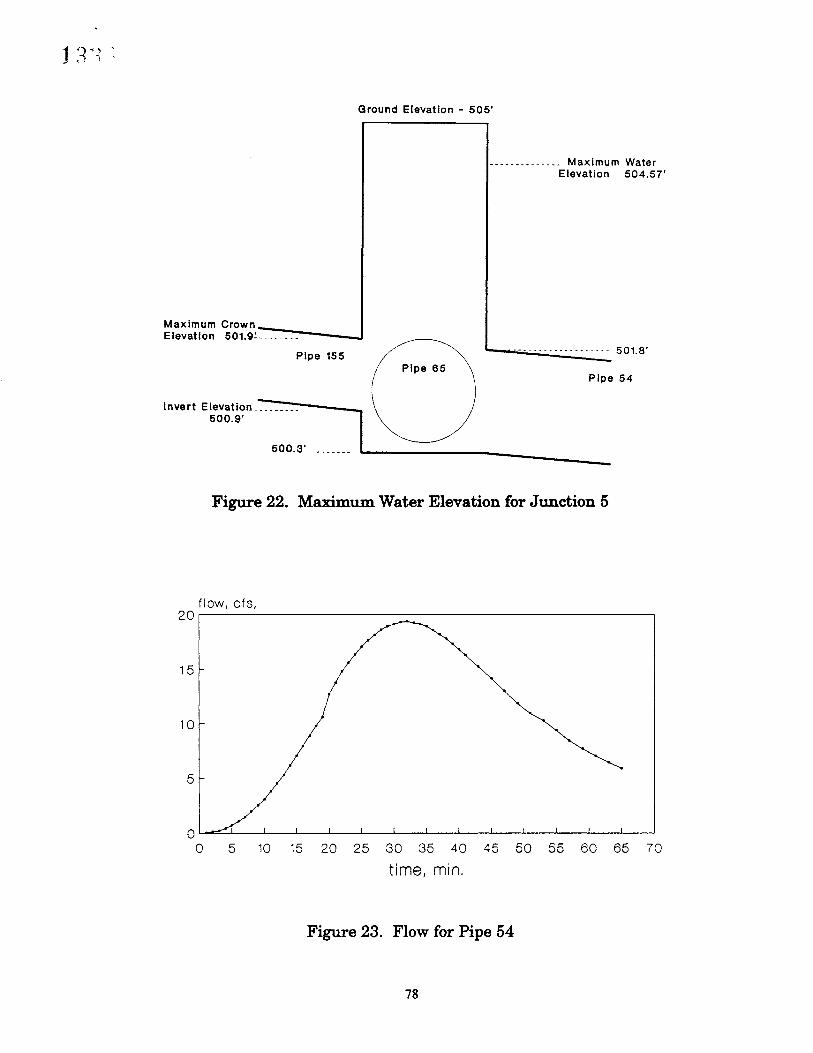
Ground Elevation - 505'
------------ __ Maximum WaterElevation 504.57'
Maximum CrownElevation 501.9~--------
Pipe 155Pipe 65
------------------- 501.8'
Pipe 54
Invert Elevation _500.9'
500.3' _
Figure 22. Maximum Water Elevation for Junction 5
flow, cfs,20~---------------------------
15
10
5
O~=__L___L____L...___L...____L...____L...____L...____"___----J"___----J_----J_ ____J"_______J"______J
o 5 10 15 20 25 30 35 40 45 50 55 60 65 70
time, min.
Figure 23. Flow for Pipe 54
78

133/
Example 3: Clark Method
The sample sewer network contains three sewers of different length, elevation, and diameter. Pipes have a Manning's n of 0.013. Inflow is provided to thesystem using the Clark method. All subareas are 60 acres and have identical timearea diagrams and storage coefficients. A tailwater elevation of 1098.5 ft is given atthe outfall. Pressurized flow run data in the PFA command include
1. 150-min simulation
2. 20-sec time step
3. lO-min print interval.
Pipe system data are listed in Table 8. The resulting input and output files appearin Tables 9 and 10.
Table 8. Clark Method Example Data
Nodes Nodes Length DiameterUpstream Downstream (ft) (in) Angle
4 3 340 48 413 2 630 48 02 1 412 60 0
79

Table 9. Clark Method Input File
0010 JOB PRESSURIZED FLOW USING CLARK METHOD0020 SWI 60030 PDA 0.013 24 3.9 2.5 2 .010040 NEW KAIGHN MOUNTAIN ROAD0050 PIP 340 1128 1122 1119.2 1113.2 -480060 PNC 43 4 5 3 1 1 O. 0 O.0070 REM TRUNK 3 TO 20080 PIP 630 1122 1108 1112.2 1101.2 -480090 PNC 32 3 1 2 1 1 30. 0 O.0100 REM TRUNK 2 TO 10110 PIP 412 1108 1099 1100.2 1093.1 -600120 PNC 21 2 1 1 4 1 o. 0 O. 1.5 1098.50130 PFA 150. 20. 10 0 0 0 0 3 35 0.05 10140 HHJ 4 3 20150 REM INFLOW HYDROGRAPHS TO JUNCTIONS0160 TAD 0.0 0.0 0.2 5.0 0.4 7.0 0.6 15.0 0.8 12.0+0170 1.0 11.0 1.2 6.0 1.4 4.0 1.6 0.00180 CHY o. 1.0 1.00190 TAD 0.0 0.0 0.2 5.0 0.4 7.0 0.6 15.0 0.8 12.0+0200 1.0 11.0 1.2 6.0 1.4 4.0 1.6 0.00210 CHY O. 1.0 1.00220 TAD 0.0 0.0 0.2 5.0 0.4 7.0 0.6 15.0 0.8 12.0+0230 1.0 11.0 1.2 6.0 1.4 4.0 1.6 0.00240 CHY o. 1.0 1.00280 END
80

Table 10. Clark Method Output File
*** PFP-HYDRA (Version of Oct. 2, 1986) ***
PRESSURIZED FLOW USING CLARK METHOD
Commands Read From File example.hda10 JOB20 SWI 630 PDA 0.013 24 3.9 2.5 2 .0140 NEW KAIGHN MOUNTAIN ROAD50 PIP 340 1128 1122 1119.2 1113.2 -4860 PNC 43 4 5 3 1 1 O. 0 O.70 REM TRUNK 3 TO 280 PIP 630 1122 1108 1112.2 1101.2 -4890 PNC 32 3 1 2 1 1 30. 0 O.
100 REM TRUNK 2 TO 1110 PIP 412 1108 1099 1100.2 1093.1 -60120 PNC 21 2 1 1 4 1 O. 0 O. 1.5 1098.5130 PFA 150. 20. 10 0 0 0 0 3 35 0.05 1140 HHJ 4 3 2150 REM INFLOW HYDROGRAPHS TO JUNCTIONS160 TAD 0.0 0.0 0.2 5.0 0.4 7.0 0.6 15.0 0.8 12.0+
1.0 11.0 1.2 6.0 1.4 4.0 1.6 0.0180 CHY o. 1.0 1.0190 TAD 0.0 0.0 0.2 5.0 0.4 7.0 0.6 15.0 0.8 12.0+
1.0 11.0 1.2 6.0 1.4 4.0 1.6 0.0210 CHY O. 1.0 1.0220 TAD 0.0 0.0 0.2 5.0 0.4 7.0 0.6 15.0 0.8 12.0+
1.0 11.0 1.2 6.0 1.4 4.0 1.6 0.0240 CHY o. 1.0 1.0280 END
END OF RUN.
81
DATE 06-21-90PAGE NO 1
133J

1 \1 - " ~_ ,_ ':l t·
Table 10. Clark Method output File, cont.
*** PFP-HYDRA (Version of Oct.2, 1986) ***
***** PRESSURIZED FLOW SIMULATIONS *****
TOTAL SIMULATION TIME IS 150 MIN.INCREMENTAL TIME IS 10 MIN.LENGTH OF INTEGRATION STEP IS 20. SECONDSINITIAL TIME .00 HOURSSURCHARGE VARIABLES: ITMAX... 35
SURTOL. • • .050PRINTED OUTPUT AT THE FOLLOWING 0 JUNCTIONS
AND FOR THE FOLLOWING 0 PIPES
82
DATE 06-21-90PAGE NO 2

Table 10. Clark Method Output File, cont.
*** PFP-HYDRA (Version of Oct.2, 1986) *** DATE 06-21-90PAGE NO 3
MAX.
PIPE LENGTH AREA MANNING WIDTH DEPTH JUNCTIONS INVERT HEIGHTNUMBER (FT) (SQ FT) COEF. (FT) (FT) AT ENDS ABOVE JUNCTIONS------ ------ ------- ------- --------- ---------------
1 43 340. 12.57 .013 4.00 4.00 4 3 .00 1.002 32 630. 12.57 .013 4.00 4.00 3 2 .00 1.003 21 412. 19.63 .013 5.00 5.00 2 1 .00 .00
83

Table 10. Clark Method Output File, cont.
*** PFP-HYDRA (Version of Oct.2, 1986) *** DATE 06-21-90PAGE NO 4
JUNCTION GROUND CROWN INVERT QINST CONNECTING PIPESNUMBER ELEV. ELEV. ELEV. (CFS)
-------- ------ ------ ----------------
1 4 1128.00 1123.20 1119.20 .00 432 3 1122.00 1117.20 1112.20 .00 43 323 2 1108.00 1105.20 1100.20 .00 32 214 1 1099.00 1098.10 1093.10 .00 21
84

Table 10. Clark Method Output File, cant.
*** PFP-HYDRA (Version of Oct.2, 1986) ***
* * * * FREE OUTFALL DATA * * * *
DATE 06-21-90PAGE NO 5
FREE OUTFLOW AT JUNCTIONS
OUTFLOW CONTROL WATER SURFACE ELEV. IS
1
1098.50 FEET
* * * * SUMMARY OF INITIAL HEADS, FLOWS AND VELOCITIES * * * *
INITIAL HEADS, FLOWS AND VELOCITIES ARE ZERO
85

Table 10. Clark Method Output File, cont.
*** PFP-HYDRA (Version of Oct.2, 1986) *** DATE 06-21-90PAGE NO 6
* * * *JUNCTION HYDROGRAPHS OBTAINED BY SCS OR CLARK METHOD* * * *
JUNCTION 4 JUNCTION 3 JUNCTION 2TIME FLOW TIME FLOW TIME FLOWHR. MIN CFS HR. MIN CFS HR. MIN CFS
o. 0 .00 o. 0 .00 o. 0 .000.22 6.36 0.22 6.36 0.22 6.360.45 33.24 0.45 33.24 0.45 33.241. 7 77.93 1. 7 77.93 1. 7 77.931.29 115.15 1.29 115.15 1.29 115.151.52 121.80 1.52 121.80 1.52 121.802.14 104.33 2.14 104.33 2.14 104.332.36 80.81 2.36 80.81 2.36 80.812.59 61.95 2.59 61.95 2.59 61.953.21 47.50 3.21 47.50 3.21 47.503.43 36.41 3.43 36.41 3.43 36.414. 6 27.90 4. 6 27.90 4. 6 27.904.28 21.36 4.28 21.36 4.28 21.364.50 16.36 4.50 16.36 4.50 16.365.13 12.52 5.13 12.52 5.13 12.525.35 9.59 5.35 9.59 5.35 9.595.58 7.35 5.58 7.35 5.58 7.356.20 5.64 6.20 5.64 6.20 5.646.42 4.32 6.42 4.32 6.42 4.327. 5 3.31 7. 5 3.31 7. 5 3.317.27 2.53 7.27 2.53 7.27 2.537.49 1.94 7.49 1.94 7.49 1.948.12 1.48 8.12 1.48 8.12 1.488.34 1.14 8.34 1.14 8.34 1.148.56 .87 8.56 .87 8.56 .879.19 .67 9.19 .67 9.19 .679.41 .51 9.41 .51 9.41 .51
10. 3 .32 10. 3 .32 10. 3 .3210.26 .14 10.26 .14 10.26 .1410.48 .00 10.48 .00 10.48 .00
86

Table 10. Clark Method Output File, cont.
*** PFP-HYDRA (Version of Oct.2, 1986) *** DATE 06-21-90PAGE NO 7
* * * * SUMMARY STATISTICS FOR JUNCTIONS * * * *
GROUND UPPERMOST FEET MAX. TIME FEET OF LENGTH/INVERT PIPE CROWN COMPUTED OF SURCHARGE OF
JUNCTION ELEV. ELEV. WATER SURFACE OCCURRENCE AT MAX. SURCHARGENUMBER (FT) (FT) ELEV HR. MIN. DEPTH (MIN)
-------- ------- ---------- ----------------------- --------- ---------
4 1128.00 1123.20 1124.45 1 52 1.25 32.001119.20
3 1122.00 1117.20 1124.36 1 29 7.16 54.331112.20
2 1108.00 1105.20 1105.98 1 52 .78 25.671100.20
1 1099.00 1098.10 1098.50 0 0 .40 150.001093.10
87

Table 10. Clark Method Output File, cont.
*** PFP-HYDRA (Version of Oct.2, 1986) *** DATE 06-21-90PAGE NO 8
* * * * SUMMARY STATISTICS FOR PIPES * * * *
PIPE MAXIMUM TIME RATIO OF MAX. DEPTH ABOVEDESIGN VERTICAL COMPUTED OF MAX. TO INVERT PIPE ENDS
PIPE FLO/VEL DEPTH FLO/VEL OCCURRENCE DESIGN UP OSNUMBER CFS/FPS (IN) CFS/FPS HR. MIN. FLOW (FT) (FT)------ ------- -------- -------- --------- -------- ---------~------
43 190.8 48.0 178.6 1 29 .9 5.25 11.1615.2 19.0
32 189.8 48.0 234.6 1 41 1.2 12.16 4.7815.1 18.7
21 341.9 60.0 355.0 1 31 1.0 5.78 5.4017.4 18.8
* * * * * PRESSURIZED FLOW SIMULATION ENDED * * * * *
88

Evaluation ofResults
This example was generated using PFP-HYDRA's design capability. The rational method triangular hydrograph provided inflow to the system for design purposes. Using identical Clark hydrographs, with a peak flow of 121.80 cfs, the system analysis was performed. All junctions surcharged.
Junction 3 has a maximum water surface elevation of 1098.5 ft, which isabove ground level. The maximum water surface elevation can be used to determine the volume of water that surcharges to the street. Table 11 shows the maximum water elevation compared to ground and crown elevations.
Table 11. Maximum Water and Crown Elevations--Clark Method Example
JunctionGroundLevel (ft)
WaterLevel (ft)
Crown Level (ft)
Upstream Downstream
4321
1128112211081099
1124.451124.361105.981098.5
1117.21105.21098.1
1123.21116.21105.2
Example 4: User Hydrographs
The North Magazine Avenue network contains six sewers with different characteristics. User-generated hydrographs provide inflow to the system. A tailwaterelevation of 1240.1 it is assumed at the outfall point. Pressurized flow data inputincludes a 2-sec time step, a total simulation time of 35 min, and six junction hydrographs for inflow. The resulting input and output files appear in Tables 12 and 13.
89

13;; .~d
Table 12. North Magazine Avenue Input File
0010 JOB North Magazine Ave.- Pressurized Flow wI User Hydrographs0020 SWI 60030 PDA .013 12 3.9 2.5 2 .0020040 NEW TRUNK LINE 511-590050 PIP 32 1253.6 1253.4 1249.4 1249.2 -180060 PNC 51159 511 5 59 1 1 90 2 0 1.5 0 0 0 0.1 0.50070 REM TRUNK LINE 59-570080 PIP 48 1253.5 1255.3 1249.1 1248.8 -180090 PNC 5957 59 1 57 1 1 50 2 0 0 0 0 0 0.1 0.50100 REM TRUNK LINE 57-550110 PIP 29 1255.3 1254.2 1248.7 1248.5 -180120 PNC 5755 57 1 55 1 1 20 2 0 0 0 0 0 0.1 0.50130 REM TRUNK LINE 55-530140 PIP 30 1254.2 1254.5 1248.4 1248.0 -180150 PNC 5553 55 1 53 1 1 70 2 0 0 0 0 0 0.1 0.50160 REM TRUNK LINE 53-510170 PIP 39 1254.5 1253.7 1247.9 1247.2 -180180 PNC 5351 53 1 51 1 1 45 2 0 0 0 0 0 0.1 0.50190 REM TRUNK LINE 51-5120300 PIP 138 1253.7 1248.6 1247.1 1244.5 -180310 PNC 51512 51 1 512 4 1 0 2 0 0 1245.7 0 0 0 0.50320 PFA 12. 2. 2 0 o. 0 0 6 30 0.05 10330 HHJ 511 59 57 55 53 510340 HHD 0.00 1.0 0.0 0.0 0.6 0.0 0.10350 HHD 0.18 4.9 2.5 0.8 4.6 4.3 0.70360 HHD 0.36 2.5 1.3 0.4 1.2 1.4 0.50370 HHD 0.54 1.0 0.5 0.2 0.7 0.0 0.10400 END
90

Table 13. North Magazine Avenue Output File
*** PFP-HYDRA (Version of Oct. 2, 1986) *** DATE 06-21-90PAGE NO 1
1348
North Magazine Ave.- Pressurized Flow wi User Hydrographs
Commands Read From File example.hda10 JOB20 SWI 630 PDA .013 12 3.9 2.5 2 .00240 NEW TRUNK LINE 511-5950 PIP 32 1253.6 1253.4 1249.4 1249.2 -1860 PNC 51159 511 5 59 1 1 90 2 0 1.5 0 0 0 0.1 0.570 REM TRUNK LINE 59-5780 PIP 48 1253.5 1255.3 1249.1 1248.8 -1890 PNC 5957 59 1 57 1 1 50 2 0 0 0 0 0 0.1 0.5
100 REM TRUNK LINE 57-55110 PIP 29 1255.3 1254.2 1248.7 1248.5 -18120 PNC 5755 57 1 55 1 1 20 2 0 0 0 a a 0.1 0.5130 REM TRUNK LINE 55-53140 PIP 30 1254.2 1254.5 1248.4 1248.0 -18150 PNC 5553 55 1 53 1 1 70 2 0 0 0 a 0 0.1 0.5160 REM TRUNK LINE 53-51170 PIP 39 1254.5 1253.7 1247.9 1247.2 -18180 PNC 5351 53 1 51 1 1 45 2 0 0 a a 0 0.1 0.5190 REM TRUNK LINE 51-512300 PIP 138 1253.7 1248.6 1247.1 1244.5 -18310 PNC 51512 51 1 512 4 1 0 2 0 0 1245.7 0 0 0 0.5320 PFA 12. 2. 2 0 o. 0 0 6 30 0.05 1330 HHJ 511 59 57 55 53 51340 HHD 0.00 1.0 0.0 0.0 0.6 0.0 0.1350 HHD 0.18 4.9 2.5 0.8 4.6 4.3 0.7360 HHD 0.36 2.5 1.3 0.4 1.2 1.4 0.5370 HHD 0.54 1.0 0.5 0.2 0.7 0.0 0.1400 END
END OF RUN.
91

12 MIN.2 MIN.
2. SECONDS
Table 13. North Magazine Avenue Output File, cont.
*** PFP-HYDRA (Version of Oct.2, 1986) ***
***** PRESSURIZED FLOW SIMULATIONS *****
TOTAL SIMULATION TIME ISINCREMENTAL TIME ISLENGTH OF INTEGRATION STEP ISINITIAL TIME .00 HOURSSURCHARGE VARIABLES: ITMAX... 30
SURTOL... .050PRINTED OUTPUT AT THE FOLLOWING 0 JUNCTIONS
AND FOR THE FOLLOWING 0 PIPES
92
DATE 06-21-90PAGE NO 2

Table 13. North Magazine Avenue Output File, cont.
*** PFP-HYDRA (Version of Oct.2, 1986) *** DATE 06-21-90PAGE NO 3
MAX.PIPE LENGTH AREA MANNING WIDTH DEPTH JUNCTIONS INVERT HEIGHT
NUMBER (FT) (SQ FT) COEF. (FT) (FT) AT ENDS ABOVE JUNCTIONS------- ------ ------- ------- --------- ---------------
1 51159 32. 1.77 .013 1.50 1.50 511 59 .00 .102 5957 48. 1.77 .013 1.50 1.50 59 57 .00 .103 5755 29. 1.77 .013 1.50 1.50 57 55 .00 .104 5553 30. 1.77 .013 1.50 1.50 55 53 .00 .105 5351 39. 1.77 .013 1.50 1.50 53 51 .00 .106 51512 138. 1.77 .013 1.50 1.50 51 512 .00 .00
93
j 3 r.- ,_ ;J J.

Table 13. North Magazine Avenue Output File, cant.
*** PFP-HYDRA (Version of Oct.2, 1986) *** DATE 06-21-90PAGE NO 4
JUNCTION GROUND CROWN INVERT QINST CONNECTING PIPESNUMBER ELEV. ELEV. ELEV. (CFS)
-------- ------ --~--- ----------------
1 511 1253.60 1250.90 1249.40 .00 511592 59 1253.50 1250.70 1249.10 .00 51159 59573 57 1255.30 1250.30 1248.70 .00 5957 57554 55 1254.20 1250.00 1248.40 .00 5755 55535 53 1254.50 1249.50 1247.90 .00 5553 53516 51 1253.70 1248.70 1247.10 .00 5351 515127 512 1248.60 1246.00 1244.50 .00 51512
94

Table 13. North Magazine Avenue Output File, cont.
*** PFP-HYDRA (Version of Oct.2, 1986) ***
* * * * FREE OUTFALL DATA * * * *
DATE 06-21-90PAGE NO 5
FREE OUTFLOW AT JUNCTIONS
OUTFLOW CONTROL WATER SURFACE ELEV. IS
512
1245.70 FEET
* * * * SUMMARY OF INITIAL HEADS, FLOWS AND VELOCITIES * * * *
INITIAL HEADS, FLOWS AND VELOCITIES ARE ZERO
95

Table 13. North Magazine Avenue Output File, cont.
*** PFP-HYDRA (Version of Oct.2, 1986) *** DATE 06-21-90PAGE NO 6
***** JUNCTION HYDROGRAPHS GIVEN BY USERS *****
JUNCTION TRIANGLE HYDROGRAPHNUMBER TIME (MIN)/INFLOW (CFS)
511 .00/ 1.00 10.80/ 4.90 21.60/ 2.50 32.40/ 1.0059 .00/ .00 10.80/ 2.50 21.60/ 1.30 32.40/ .5057 .00/ .00 10.80/ .80 21.60/ .40 32.40/ .2055 .00/ .60 10.80/ 4.60 21.60/ 1.20 32.40/ .7053 .00/ .00 10.80/ 4.30 21.60/ 1.40 32.40/ .0051 .00/ .10 10.80/ .70 21.60/ .50 32.40/ .10
96

Table 13. North Magazine Avenue Output File, cont.
*** PFP-HYDRA (Version of Oct.2, 1986) *** DATE 06-21-90PAGE NO 7
* * * * SUMMARY STATISTICS FOR JUNCTIONS * * * *
GROUND UPPERMOST FEET MAX. TIME FEET OF LENGTH/INVERT PIPE CROWN COMPUTED OF SURCHARGE OF
JUNCTION ELEV. ELEV. WATER SURFACE OCCURRENCE AT MAX. SURCHARGENUMBER (FT) (FT) ELEV HR. MIN. DEPTH (MIN)
-------- ------- ---------- --------------~-------- --------- ---------
511 1253.60 1250.90 1252.49 0 11 1.59 1.301249.40
59 1253.50 1250.70 1252.39 0 11 1.69 1.331249.10
57 1255.30 1250.30 1252.07 0 11 1.77 1.601248.70
55 1254.20 1250.00 1251.84 0 11 1.84 1.901248.40
53 1254.50 1249.50 1251.36 0 11 1.86 2.231247.90
51 1253.70 1248.70 1250.25 0 11 1.55 2.331247.10
512 1248.60 1246.00 1246.00 0 11 .00 .001244.50
97

Table 13. North Magazine Avenue Output File, cont.
*** PFP-HYDRA (Version of Oct.2, 1986) *** DATE 06-21-90PAGE NO 8
* * * * SUMMARY STATISTICS FOR PIPES * * * *
PIPE MAXIMUM TIME RATIO OF MAX. DEPTH ABOVEDESIGN VERTICAL COMPUTED OF MAX. TO INVERT PIPE ENDS
PIPE FLO/VEL DEPTH FLO/VEL OCCURRENCE DESIGN UP DSNUMBER CFS/FPS (IN) CFS/FPS HR. MIN. FLOW (FT) (FT)------ ------- -------- -------- --------- -------- ----------------51159 8.3 18.0 5.1 0 11 .6 3.09 3.19
4.7 4.3
5957 8.3 18.0 7.7 0 11 .9 3.29 3.274.7 5.3
5755 8.7 18.0 8.5 0 11 1.0 3.37 3.344.9 5.5
5553 12.1 18.0 13.2 0 11 1.1 3.44 3.366.9 7.5
5351 14.1 18.0 17.5 0 11 1.2 3.46 3.058.0 9.9
51512 14.4 18.0 18.2 0 11 1.3 3.15 1.508.2 10.3
* * * * * PRESSURIZED FLOW SIMULATION ENDED * * * * *
98

Evaluation ofResults
The summary printout of pressurized flow shows all junctions except Junction 512 (outfall) surcharging. Pipes 5755, 5553, 5351, and 51512 experience pressurized flow conditions. A comparison of maximum water elevation and crown elevation for each junction shows which pipe entry and exits are surcharged (see Table14). This method helps to determine the accuracy of the surcharge and pressurizedflow conditions.
Table 14. Maximum Water and Crown ElevationsNorth Magazine Avenue Example
JunctionMaximum Water
Elevation (ft)Crown Elevation (ft)
Upstream Downstream
5115957555351512
1252.491252.391252.071251.841251.361250.251246.00
99
1250.91250.31250.01249.51248.71246.0
1250.91250.61250.21249.91249.41248.6


REFERENCES
Brater, E. F., & King, H. W. (1976). Handbook ofhydraulics for the solution ofhydraulic engineering problems (6th ed.). New York: McGraw-Hill.
GKY & Associates, Inc. (1986). PFP-HYDRA user's manual-Draft. Springfield,VA: Author.
Ponce, V. M. (1989). Engineering hydrology principles and practices. EnglewoodCliffs, NJ: Prentice-Hall.
U.S. Department of Agriculture. Soil Conservation Service. (1986). Urban hydrology for small watersheds (Technical Release No. 55). Washington, DC: Author.
Viessman, W., Jr.; Lewis, G. L.; & Knapp, J. W. (1989). Introduction to hydrology(3rd ed.). New York: Harper & Row.
Yu, S. L., & Wu, Y: (1989). A microcomputer model for simulating pressurized flowin a storm sewer system (VTRC Report No. 89-R21). Charlottesville:Virginia Transportation Research Council.
101


APPENDIX A
Calculations and Troubleshooting


CALCULATIONS
Determination of Time Step
Using the f91lowing equation
find the shortest pipe with the largest diameter and plug the values in. For example, you have a 50-ft pipe of diameter 36 in (3 ft). The acceleration due to gravity is32.2 ftlsec2• The allowable time-step calculation would be
At =. 50 ft = 5.0872 sec./32.2 ft/sec2 x 3 it
You would enter the value 5.0 sec into the program through the PFA command. Ifmore detailed calculations are desired, then a smaller number may be input. If anumber larger than 5 sec is input, the program will calculate a new time step because the stability criteria will have been violated.
Determination of Parameters for SCS Unit Hydrograph Method
1. Finding the SCS curve number.
The area to be designed for is mostly paved parking lot, with some trees andgrass. The two categories for curve numbers might be:
• open space, poor condition, curve number =79
• paved parking lot, curve number = 98.
The design area is in Charlottesville, Albemarle County, Virginia. Using BCS Technical Release No. 55, we find the soil type to be Cecil Loam, which is hydrologic condition B (Table B2, Appendix B).
This allows the user of the charts in Appendix B to determine the curve num-bers.
60 47.440 + 39.2
New curve number = 86.6
Curve Number x % Area% Area
The curve number for use is, then, a composite of the previous two numbers.The composite number is calculated as follows:
CurveNumber (CN)
7998
105

2. Choosing a rainfall.
Use a developed IDF curve to determine storm duration and depth, or useyour own knowledge to force the conditions you desire.
3. Choosing a length to divide.
You may use
1. distance to point within area with longest travel time
2. distance to centroid of area.
It is recommended that the larger of these two values be used.
Determination of Time-Area Diagram
Using a topographical map of the area, calculate travel times from variouspoints within the watercourse area to the outfall point. For example, with an areaof 600 acres in the Virginia mountains:
Point 1. Distance to outfall =729 11;
Average watercourse slope =80 ftl729 it =0.109, or 11%
Using Figure B1 in Appendix B, for forest with sheet flow, the velocity is graphically determined to be 0.7 ftlsec. Multiply the velocityby the distance, and the travel time is 529 sec, or 8.5 min.
Continue this for several points to define the area and then separate the area intoequal times as in Figure 3. After a maximum of 300 ft, sheet flow usually becomesshallow concentrated flow. The average velocity for this flow can be determinedfrom Figure B2 in Appendix B.
The lines separating the area are called isochrones. Find the area within theisochrones and construct a time-area histogram.
TROUBLESHOOTING
Example 1: Design Flow Equal to Zero
If you get a design flow equal to zero (see Table AI), check your invert height!The invert must be input in such a way that this will not happen (see Table A2).
106

Table A1. Incorrect Output Using North Magazine Avenue Example
1 () f" 0
J_ \.1 t1. '.
*** PFP-HYDRA (Version of Oct.2, 1986) *** DATE 11-15-90PAGE NO 8
* * * * SUMMARY STATISTICS FOR PIPES * * * *
PIPE MAXIMUM TIME RATIO OF MAX. DEPTH ABOVEDESIGN VERTICAL COMPUTED OF MAX. TO INVERT PIPE ENDS
PIPE FLO/VEL DEPTH FLO/VEL OCCURRENCE DESIGN UP DSNUMBER CFS/FPS (IN) CFS/FPS HR. MIN. FLOW (FT) (FT)------- _...~---~ --------- -------- ---------- ---~..._-- ----_.-._----~----
51159 8.3 18.0 1.3 0 1 .2 .41 .344.7 3.4
5957 8.3 18.0 1.5 0 1 .2 .44 .514.7 3.3
5755 OJ 18.0 1.5 0 1 .0 .61 .15.0 2.6
5553 12.1 18.0 2.4 0 1 .2 .45 .356.9 5.3
5351 14.1 18.0 2.7 0 1 .2 .45 .348.0 6.2
51512 14.4 18.0 2.6 0 1 .2 .44 1.208.2 2.6
* * * * * PRESSURIZED FLOW SIMULATION ENDED * * * * *
107

Table A2. Incorrect Input Using North Magazine Avenue Example
0010 JOB North Magazine Ave.- Pressurized Flow wi User Hydrographs0020 SWI 60030 PDA .013 12 3.9 2.5 2 .0020040 NEW TRUNK LINE 511-590050 PIP 32 1253.6 1253.4 1249.4 1249.2 -180060 PNC 51159 511 5 59 1 1 90 2 0 1.5 0 0 0 0.1 0.50070 REM TRUNK LINE 59-570080 PIP 48 1253.5 1255.3 1249.1 1248.8 -180090 PNC 5957 59 1 57 1 1 50 2 0 0 0 0 a 0.1 0.50100 REM TRUNK LINE 57-550110 PIP 29 1255.3 1254.2 [-1-2-48-.-7-1-2-48-.7-{-180120 PNC 5755 57 1 55 1 1 20 2 0 0 0 0 0 0.1 0.50130 REM TRUNK LINE 55-530140 PIP 30 1254.2 1254.5 1248.4 1248.0 -180150 PNC 5553 55 1 53 1 1 70 2 0 0 0 0 0 0.1 0.50160 REM TRUNK LINE 53-510170 PIP 39 1254.5 1253.7 1247.9 1247.2 -180180 PNC 5351 53 1 51 1 1 45 2 0 0 0 0 0 0.1 0.50190 REM TRUNK LINE 51-5120300 PIP 138 1253.7 1248.6 1247.1 1244.5 -180310 PNC 51512 51 1 512 4 1 0 2 0 0 1245.7 0 0 0 0.50320 PFA 1. 2. 2 0 o. 0 a 6 30 0.05 10330 HHJ 511 59 57 55 53 510340 HHD 0.00 1.0 0.0 0.0 0.6 0.0 0.10350 HHD 0.18 4.9 2.5 0.8 4.6 4.3 0.70360 HHD 0.36 2.5 1.3 0.4 1.2 1.4 0.50370 HHD 0.54 1.0 0.5 0.2 0.7 0.0 0.10400 END
108

Example 2: Warning in the Output and Hydraulic Gradeline Equal to Zero
If there is a warning in the output that reads:
**** WARNING **** icyc = 306 ZERO SURFACE AREA
(see Table A3), then check the difference between the crown elevation of incomingpipe and the invert elevation of outgoing pipe at a particular junction (i.e., difference =crown elevation - invert elevation). Adjust and make the difference greaterthan or equal to zero.
If the hydraulic gradeline goes to zero and jumps back up 5 ft (see Table A3),then check the input file (see Table A4) for the tailwater elevation. Add or adjustthe tailwater elevation, and check the invert and crown levels to obtain reasonableresults.
109

Table A3. Incorrect Output Using Clark Method Example
*** PFP-HYDRA (Version of Oct.2, 1986) *** DATE 11-14-90PAGE NO 9
CYCLE 270 TIME 1 HRS - 30.00 MIN
JUNCTIONS / DEPTHS
4/ 5.70* 3/ 8.70* 2/ 8.35* 1/ 5.00
CONDUITS / FLOWS
43/ 88.60 32/ 232.16***** WARNING ***** ICYC= 300
COMPUTED AT JUNCTION 2CHECK INPUT DATA FOR HIGH PIPE
21/ 394.21 90004/ 394.21ZERO SURFACE AREA
CYCLE 300 TIME 1 HRS - 40.00 MIN
JUNCTIONS / DEPTHS
4/ 5.70* 3/ 8.70* 2/ 18.99 1/ .00
CONDUITS / FLOWS
43/ 88.60 32/ 234.53***** WARNING ***** ICYC= 306
COMPUTED AT JUNCTION 2CHECK INPUT DATA FOR HIGH PIPE
***** WARNING ***** ICYC= 311COMPUTED AT JUNCTION 2-CHECK INPUT DATA FOR HIGH PIPE
***** WARNING ***** ICYC= 316COMPUTED AT JUNCTION 2CHECK INPUT DATA FOR HIGH PIPE
21/ .00 90004/ZERO SURFACE AREA
ZERO SURFACE AREA
ZERO SURFACE AREA
.00
CYCLE 330 TIME 1 HRS - 50.00 MIN FLOW DIFF. IN SURCHARGED AREA= -3.55ITERATIONS REQUIRED= 1
JUNCTIONS / DEPTHS
4/ 5.70* 3/ 8.24* 2/ 8.67* 1/ 5.00
CONDUITS / FLOWS
43/ 91.52 32/ 233.01 21/ 376.16
110
90004/ 376.16

Table A3. Incorrect Output Using Clark Method Example, cant.
*** PFP-HYDRA (Version of Oct.2, 1986) *** DATE 11-14-90PAGE NO 11
* * * * TIME HISTORY OF HYDRAULIC GRADELINE(VALUES IN FEET)
* * * *
JUNCTION 4 JUNCTION 3 JUNCTION 2TIME GRND 1128.00 GRND 1122.00 GRND 1108.00
HR.MIN ELEV DEPTH ELEV DEPTH ELEV DEPTH
0.10 1122.66 .36 1113.87 .57 1097.96 .760.20 1122.81 .51 1114.11 .81 1098.28 1.080.30 1123.14 .84 1114.47 1.17 1098.74 1.540.40 1123.45 1.15 1114.98 1.68 1099.41 2.210.50 1123.78 1.48 1115.45 2.15 1100.02 2.821. 0 1124.18 1.88 1115.96 2.66 1100.65 3.451.10 1124.59 2.29 1116.54 3.24 1101.42 4.221.20 1128.00 3.00 1121.08 6.00 1108.00 8.001.30 1128.00 3.00 1122.00 6.00 1105.55 8.001.40 1128.00 3.00 1122.00 6.00 1116.19 8.001.50 1128.00 3.00 1121.54 6.00 1105.87 8.002 • 0 1128.00 3.00 1120.13 6.00 1097.20 GO2.10 1128.00 3.00 1119.66 6.00 1097.20 .002.20 1127.70 3.00 1122.00 6.00 1097.20 .002.30 1125.18 2.88 1119.18 5.88 1102.82 5.62
III

Table A4. Incorrect Input Using Clark Method Example
0010 JOB PRESSURIZED FLOW USING CLARK METHOD0020 SWI 60030 PDA 0.013 24 3.9 2.5 2 .010040 NEW KAIGHN MOUNTAIN ROAD0050 PIP 340 1128 1122 1122.3 1116.3 -360060 PNC 43 4 5 3 1 1 O. 0 O.0070 REM TRUNK 3 TO 20080 PIP 630 1122 1108 1113.3 1101.2 -480090 PNC 32 3 1 2 1 1 30. 0 O.0100 REM TRUNK 2 TO 10110 PIP 412 1108 1099 1097.2 1091.1 -600120 PNC 21 2 1 1 4 1 O. 0 O.0130 PFA 150. 20. 10 2 0 3 3 3 30 0.05 10131 PFP 43 32 210132 PHJ 4 3 20140 HHJ 4 3 20150 REM INFLOW HYDROGRAPHS TO JUNCTIONS0160 TAD 0.0 0.0 0.2 5.0 0.4 7.0 0.6 15.0 0.8 12.0+0170 1.0 11.0 1.2 6.0 1.4 4.0 1.6 0.00180 CHY o. 1.0 1.00190 TAD 0.0 0.0 0.25 10.0 0.5 26.0 0.75 29.0+0200 1.0 14.0 1.25 3.0 1.5 0.00210 CHY o. 1.0 1.00220 TAD 0.0 0.0 0.25 10.0 0.5 26.0 0.75 27.5+0230 1.0 12.0 1.25 0.00240 CHY O. 1.0 1.00280 END
112

APPENDIXB
SCS Curve Number and Overland Velocity Charts


j 3t"'f I- _. It)
Table Bl. Runoff Curve Numbers for Urban Areas l
Cover descriptionCurve numbers tor
hydrologic soil group-
Cover type and hydrologic conditionAverage percentimpervious area2 A 8 c o
Fully developed urban areas (vegetation established)
Open space (lawns, parks, golt courses, cemeteries, etc.)3:Poor condition (grass cover < 500/0) . ...................... 68 79 86 89Fair condition (grass cover 500/0 to 750/0) ................... 49 69 79 84Good condition (grass cover> 750/0) ...................... 39 61 74 80
Impervious areas:Paved parking lots, roofs, driveways, etc. (excluding right-ot-
way)................................................. 98 98 98 98Streets and roads:
Paved; curbs and storm sewers (excluding right-at-way). ...... 98 98 98 98Paved; open ditches (including right-of-way)................. 83 89 92 93Gravel (including right-at-way) ............................ 76 85 89 91Dirt (including right-at-way) ............................... 72 82 87 89
Western desert urban areas:Natural desert landscaping (pervious areas only).4 ............ 63 77 85 88Artificial desert landscaping (impervious weed barrier, desert
shrub with 1- to 2-inch sand or gravel mulch and basin bord-ers).................................................. 96 96 96 96
Urban districts:Commercial and business .................................... 85 89 92 94 95Industrial .......................................................... 72 81 88 91 93
Residential districts by average lot size:1/8 acre or less (town houses) ............................ 65 77 85 90 921/4 acre .............................................. 38 61 75 83 871/3 acre ................................................................................. 30 57 72 81 861/2 acre .............................................. 25 54 70 80 851 acre 20 51 68 79 842 acres ............................................... 12 46 65 77 82
Developing urban areas
Newly graded areas (pervious areas only, no vegetation).5 77 86 91 94Idle lands (eN's are determined using cover types similar to those
in table 2-2a).
1 Average runoff condition, la = 0.25.2 The average percent impervious area shown was used to develop the composite CN's. Other assumptions are as follows: impervious areas are directly connected to the drainage system,impervious areas have a CN of 98, and pervious areas are considered equivalent to open space in good hydrologic condition.
3CN's shown are equivalent to those of pasture. Composite CN'smay be computed for other combinations of open space covertype.
"Composite CN's for natural desert landscaping should be computed based on the impervious area (CN = 98) and the perviousarea CN. The pervious area CN's are assumed equivalent todesert shrub in poor hydrologic condition.
S Composite CN's to use for the design of temporary measuresduring grading and construction should be computed using thedegree of development (impervious area percentage) and theCN's for the newly graded pervious areas.
Source: U.S. Department of Agriculture. Soil Conservation Service. (1986). Urbanhydrology for small watersheds (Technical Release No. 55). Washington, DC: Author.
lIS

1_ 3to, ,~t
Table B2. Runoff Curve Numbers for Cultivated Agricultural Lands1
Curve numbers forCover description hydrologic soil group-
HydrologicCover type Treatment2 condition3 A B C 0
Fallow Bare soil 77 86 91 94Crop residue cover (CR) Poor 76 85 90 93
Good 74 83 88 90
Row crops Straight row Poor 72 81 88 91Good 67 78 85 89
Straight row + CR Poor 71 80 87 90Good 64 75 82 85
Contoured (C) Poor 70 79 84 88Good 65 75 82 86
Contoured + CR Poor 69 78 83 87Good 64 74 81 85
Contoured & terraced (C&T) Poor 66 74 80 82Good 62 71 78 81
Contoured & terraced + CR Poor 65 73 79 81Good 61 70 77 80
Small grain Straight row Poor 65 76 84 88Good 63 75 83 87
Straight row + CR Poor 64 75 83 86Good 60 72 80 84
Contoured Poor 63 74 82 85Good 61 73 81 84
Contoured + CR Poor 62 73 81 84Good 60 72 80 83
Contoured & terraced Poor 61 72 79 82Good 59 70 78 81
Contoured & terraced + CR Poor 60 71 78 81Good 58 69 77 80
Close-seeded Straight row Poor 66 77 85 89or broadcast Good 58 72 81 85legumes or Contoured Poor 64 75 83 85rotation Good 55 69 78 83meadow Contoured & terraced Poor 63 73 80 83
Good 51 67 76 80
1 Average runoff condition. grass or close-seeded legumes in rotations, (d) percent of2Crop residue cover (CR) applies only if residue is on at least 5% residue cover on the land surface (good ~ 20% ), and (e) degreeof the surface throughout the year. of surface roughness.
3 Hydrologic condition is based on combination of factors that af- Poor: Factors impair infiltration and tend to increase runoff.fect infiltration and runoff, including (a) density and canopy of Good: Factors encourage average and better than average in-vegetative areas, (b) amount of year-round cover, (c) amount of filtration and tend to decrease runoff.
Source: U.S. Department of Agriculture. Soil Conservation Service. (1986). Urbanhydrology for small watersheds (Technical Release No. 55). Washington, DC: Author.
116

Table B3. Runoff Curve Numbers for Other Agricultural Lands!
Cover description
Cover type
Pasture, grassland, or range-continuousforage for grazing.2
Meadow-continuous grass, protected fromgrazing and generally mowed for hay.
Brush-brush-weed-grass mixture with brushthe major element.3
Woods-grass combination (orchardor tree farm). 5
Woods6
Farmsteads-buildings, lanes, driveways,and surrounding lots.
1 Average runoff condition.2 Poor: < 500/0 ground cover or heavily grazed with no mulch.Fair: 500/0 to 750/0 ground cover and not heavily grazed.Good: > 75% ground cover and lightly or only occasionallygrazed.
3 Poor: < 500/0 ground cover.Fair: 50 to 750/0 ground cover.Good: > 75% ground cover.
4 Actual curve number is less than 30; use CN = 30 for runoffcomputations.
sCN's shown were computed for areas with 500/0 woods and 500/0grass (pasture) cover. Other combinations of conditions may becomputed from the eN's for woods and pasture.
6 Poor: Forest, litter, small trees, and brush have been destroyedby heavy grazing or regular burning.Fair: Woods are grazed but not burned, and some forest littercovers the soil.Good: Woods are protected from grazing, and litter and brushadequately cover the soil.
Curve numbers forhydrologic soil group-
Hydrologiccondition A 8 C D
Poor 68 79 86 89Fair 49 69 79 84
Good 39 61 74 80
30 58 71 78
Poor 48 67 77 83Fair 35 56 70 77
Good 304 48 65 73
Poor 57 73 82 86Fair 43 65 76 82
Good 32 58 72 79
Poor 45 66 77 83Fair 36 60 73 79
Good 304 55 70 77
59 74 82 86
Source: U.S. Department of Agriculture. Soil Conservation Service. (1986). Urbanhydrology for small watersheds (Technical Release No. 55). Washington, DC: Author.
117

Table B4. Runoff Coefficients for Rational Method 0
Description of Area
BusinessDo\vntown areasNeighborllood areas
Residel1tialSingle-f~lnlily areas~111Itiunit", cletachedMultiunits, attached
Residential (suburban)Apartnlent dwelling areasI ndllstrial
Light areasHeavy areas
Parks, cenleteriesPlaygroul1clsRailroC:lcl yard areasUninlpro\'cd areasStreets
AsphalticConcreteBrick
Drives anci \valksRoofsLa\vns; Sanely Soil:
l~lat, 20/0Average, 2-7lkSteel), 70/0
La\vns; I-lea,,)' Soil:Flat, 20/0Average, 2-7o/cSteep, 70/0
RunoffCoefficients
0.70-0.950.50-0.70
0.30-0.500.40-0.600.60-0.750.25-0.400.50-{).70
0.50-0.80O.60-D.900.10-0.250.20-0.35O.20-{) ...tOO.lO-{).:30
0.70-0.950.80-0.950.70-0.85(l.75-0.B5().75-0.95
0.05-0.100.1 0-0.1.50.15-0.20
O.13-(J.170.18-0.220.25-0.35
Source: U.S. Department ofAgriculture. Soil Conservation Service. (1986). Urbanhydrology for small watersheds (Technical Release No. 55). Washington, DC: Author.
118

JIF
-, 7, 7
I ~ I
. ~ "'-_--"-"""'7..................""""I-..t.~Vu-.J~V..u..l...LJ.LJ.I_.J./J.--.L.-J.---1-.L....L-J...L.~J..U..LJ.JUJ..._--I..----J.5
.1 .2.3.5 I 2 3 5 10 20
VELOCITY, V (FT / SEC)'
Figure B1. Average Velocities for Estimating Travel Time. Source: Federal Highway Administration. (1984). Hydrology (FHWA Report No. IP-84-15). Springfield, VA: National Technical Information Service.
119

I20
I I I I I I
2 4 6 10Average velocity, ft/sec
•,~, II. ••
~ IIr
lJII II
~ IJ Ir ,
lJ ~
~ ~,IJ
If IJIJ IJ
Ii ~IJF ~
~
II
1..4
" J, I~
.4 I, ,,'I ,
II
•1# ~,
I~ II,~
J r, ljJ ~", ,
J j
"t)' jr
~I---bf~ ~Q.J
~~ Q.~I~ II
V I)J .4, If
J" j
I Ifl I
.20 -
.50 -
.01 -
.005 I
1
~ .10 -Co+-"-~Co+-
..<U
.06c. -0r--en
cuen .04S- -::s0uS-Ol.....cs
::;c
•02 -
Figure B2. Average Velocities for Estimating Travel Time for Shallow Concentrated Flow. Source: Federal Highway Administration. (1984). Hydrology(FHWA Report No. IP-84-15). Springfield, VA: National Technical InformationService.
120