1

Context-aware Telco Outdoor LocalizationYige Zhang, Weixiong Rao, Mingxuan Yuan, Jia Zeng and Pan Hui

F

Abstract—Recent years have witnessed the fast growth in telecommu-nication (Telco) techniques from 2G to upcoming 5G. Precise outdoorlocalization is important for Telco operators to manage, operate andoptimize Telco networks. Differing from GPS, Telco localization is atechnique employed by Telco operators to localize outdoor mobile de-vices by using measurement report (MR) data. When given MR samplescontaining noisy signals (e.g., caused by Telco signal interference andattenuation), Telco localization often suffers from high errors. To thisend, the main focus of this paper is how to improve Telco localizationaccuracy via the algorithms to detect and repair outlier positions withhigh errors. Specifically, we propose a context-aware Telco localizationtechnique, namely RLoc, which consists of three main components: amachine-learning-based localization algorithm, a detection algorithm tofind flawed samples, and a repair algorithm to replace outlier localizationresults by better ones (ideally ground truth positions). Unlike most exist-ing works to detect and repair every flawed MR sample independently,we instead take into account spatio-temporal locality of MR locationsand exploit trajectory context to detect and repair flawed positions. Ourexperiments on the real MR data sets from 2G GSM and 4G LTE Telconetworks verify that our work RLoc can greatly improve Telco locationaccuracy. For example, RLoc on a large 4G MR data set can achieve32.2 meters of median errors, around 17.4% better than state-of-the-art.

1 INTRODUCTION

Outdoor localization systems have gained focus recently due to theremarkable proliferation of telecommunication (Telco) networks(from 2G to upcoming 5G networks) and sensor-rich smart mo-bile devices. These systems span different application domains,such as navigation systems, location-based advertisements, socialnetworks and resource allocation in wireless networks [25]. Inparticular, Telco operators have strong interest in localizationtechnology due to their needs for automated network management,operation and optimization. Specifically, location information ofmobile devices is important for Telco operators to 1) identifylocation hotspots for capacity planning, 2) identify gaps in radiofrequency coverage, 3) troubleshoot network anomalies, and 4)locate users in emergency situations (E911) [29].

Differing from GPS, Telco localization is a technique em-ployed by Telco operators to localize outdoor mobile devices by

• Yige Zhang and Weixiong Rao are with School of Software En-gineering, Tongji University, Shanghai, China. E-mail: yigezhang,wxrao@tongji.edu.cn

• Mingxuan Yuan and Jia Zeng are with Huawei Noahs Ark Lab, HongKong. E-mail: mingxuan.yuan, jia.zeng@huawei.com

• Pan Hui is with Department of Computer Science and Engineering, HongKong University of Science and Technology, and Department of ComputerScience, University of Helsinki. E-mail: panhui@cse.ust.hk

using measurement report (MR) data. MR data mainly containthe connection information, such as signal strength, betweenmobile devices and nearby base stations. Telco operators exploit abackend localization algorithm on MR data to infer the locationsof mobile devices. Due to the rich commercial opportunities ofthe inferred locations, Telco localization has recently attractedintensive research interests in both academia [3], [40], [22] andTelco industries [29], [34], [45], [41].

Unfortunately, the design of an accurate Telco localizationalgorithm is challenging. For example, high buildings in urbancities often cause Telco signal interference and attenuation. Mobiledevices located in those areas with high buildings often generatenoisy MR samples containing unstable signal strength. Whengiven such MR samples, Telco localization cannot achieve high ac-curacy. Though the recently popular data-driven localization [22],[45], [8] leverages those MR samples tagged by GPS coordinatesto train a machine-learning-based localization model, the localiza-tion accuracy is around 80 meters in terms of median errors [45],leading to little chance of achieving GPS-like performance [8].

In this paper, we propose a context-aware Telco localizationtechnique, namely RLoc, in order to achieve high localizationaccuracy. Our work is motivated by the following observation.For those MR samples containing noisy signals, their predictedpositions are typically with high errors and significantly degradeoverall localization accuracy. For simplicity, the samples leadingto high errors are called flawed samples, and correspondingpredicted locations with high errors are called flawed locations.To this end, the main focus of this paper is how to improve Telcolocalization accuracy via the algorithm to detect flawed samplesand repair flawed positions. That is, we would like to first detectflawed MR samples. If the associated flawed positions can berepaired by highly precise ones (ideally ground truth positions),we then have chance to achieve much lower localization errors.Nevertheless, most existing works detect each individual flawedsample and then repair the corresponding flawed position [14],[27], [43], [26] and do not take into account contextual knowledgeof neighbouring MR positions. Unlike these works, we considerthat a sequence of MR positions exhibits spatio-temporal localityand contributes to a trajectory of positions. For example, whena mobile device is moving around high buildings and suffersfrom Telco signal interference, we assume that a sequence ofgenerated MR samples is all flawed. By exploiting the spatio-temporal context in the trajectory of MR positions, we design thesequence-based detect and repair approach for much lower errors.As a summary, we make the following contributions.• Confidence-based detection algorithm: Based on the physical

distance between predicted position and real ones, we definea confidence level for an MR sample to determine whether or

arX

iv:2

108.

1065

1v1

[cs

.NI]

24

Aug

202

1

2

not the sample is flawed. Beyond that, we are interested inthe confidence levels of a sequence of MR samples. Thus, wepropose a dual-stage adaptive Hidden Markov Model, calledDA-HMM, to predict a corresponding sequence of confidencelevels. By introducing the adaptive state transition probabilityand adaptive mission probability, DA-HMM can processreal world MR sequences (which exhibit uneven timestampintervals among neighbouring MR samples), and thus lead tobetter performance than traditional HMM models.

• Joint probability-based repair algorithm: Still when given asequence of flawed MR samples, we are interested in notonly the goodness of a certain candidate position to repair anindividual flawed position, but also the transition possibilityfrom the previous position to the next one. Thus, we definethe joint probability of an entire path to connect candidatepositions. Among all possible paths of candidate positions,we design a dynamic planning algorithm to select the bestone to repair the entire sequence of flawed positions.

• Extensive Performance Validation: Our experiments on thereal MR data sets from 2G GSM and 4G LTE Telco networksverify that our work RLoc greatly improves Telco locationaccuracy. For example, RLoc on a large 4G MR data set canachieve 32.2 meters of median error. Such numbers indicatethat RLoc achieves comparable accuracy as GPS.

The rest of this paper is organized as follows. Section 2 firstreviews the background and related work. Section 3 then formu-lates the problem definition and highlights the solution. Next,Sections 4 and 5 describe the detection and repair algorithms,respectively. After that, Section 6 evaluates our work. Section 7finally concludes the paper. Table 1 summarizes the mainly usedterms/symbols and associated meanings.

TABLE 1Used Terms and Associated Meanings

Term/Symbol MeaningMR Measurement ReportRSSI Radio Signal Strength IndexTelco TelecommunicationHMM Hidden Markov ModelDA-HMM A Dual-stage Adaptive Hidden Markov Modelr MR sampleLp(r) Predicted location of MR sample rLt(r) Ground truth location of MR sample rR = r1, ..., r|S| a sequence of |R| MR samplesL Telco localization modelC Confidence modelD Original Training dataset with D = DL ∪ DCDL Training subset for localization LDC Training subset for confidence model CD Testing dataset with D = D− ∪D+

D− Flawed Testing datasetsD+ Non-Flawed Testing datasetsA = ai,j State transition probability in HMMB = bj(k) Emission probability in HMMa∆ Adaptive state transition prob. by time interval ∆bγ Adaptive emission prob. by sample size γ

vk = vbsk , vssk

MR observation vk with a pair of base stations vbskand Telco signal strength vssk

2 BACKGROUND AND RELATED WORK

2.1 Background of MR Data

A Measurement Report (MR) sample maintains the connectionstate of a certain mobile device in a Telco network, includinga unique ID (IMSI: International Mobile Subscriber Identity),

connection time stamp (MRTime), up to 7 nearby base stations(RNCID and CellID) [35], and corresponding signal measure-ments such as AsuLevel, SignalLevel and RSSI. Table 2 givesan example 2G GSM MR sample collected by an Android device.AsuLevel, i.e., Arbitrary Strength Unit Level, is an integer pro-portional to the received signal strength measured by the mobiledevice. SignalLevel indicates the power ratio (typically logarithmvalue) of the output signal of the device and the input signal. RSSIdenotes a radio signal strength indicator. Among the up to 7 basestations, one of them is selected as the primary serving station toprovide communication and data services for mobile devices.

TABLE 2An Example of 2G GSM MR Record Collected by an Android Device.

MRTime *** IMSI *** SRNC ID 6188 BestCellID 26050 # BS 7RNCID 1 6188 CellID 1 26050 AsuLevel 1 18 SignalLevel 1 4 RSSI 1 -77RNCID 2 6188 CellID 2 27394 AsuLevel 2 16 SignalLevel 2 4 RSSI 2 -81RNCID 3 6188 CellID 3 27377 AsuLevel 3 15 SignalLevel 3 4 RSSI 3 -83RNCID 4 6188 CellID 4 27378 AsuLevel 4 15 SignalLevel 4 4 RSSI 4 -83RNCID 5 6182 CellID 5 41139 AsuLevel 5 16 SignalLevel 5 4 RSSI 5 -89RNCID 6 6188 CellID 6 27393 AsuLevel 6 9 SignalLevel 6 3 RSSI 6 -95RNCID 7 6182 CellID 7 26051 AsuLevel 7 9 SignalLevel 7 3 RSSI 7 -95

Generally, we can collect MR samples from two typical datasources: 1) the data collected from client side and 2) the onefrom backend Telco operators. MR samples, no matter generatedby either 4G LTE networks or from 2G GSM networks, followthe same data format if they are collected by Android APIs.Nevertheless, the data format of MR samples collected by backendTelco operators may differ from the one by frontend Android APIs(The detail refers to [20]). All these MR samples provide usefuldata collection sources. Due to the difference between MR dataformats by frontend Android devices and backend Telco operators,we use those MR feature items, e.g., RSSI, that appear within alldata sets without loss of generality.

2.2 Related Work on Telco LocalizationDepending upon location results, we category literature works intosingle-point-based and sequence-based localization. The formerworks independently process every MR sample to localize an out-door mobile device, and the latter ones frequently take as input asequence of MR samples and then leverage the underlying spatio-temporal locality of such MR samples to generate a trajectory ofpredicted locations.

2.2.1 Single-point-based Telco localizationIn terms of single-point-based localization, we classify literatureworks into two categories. Firstly, the distance-based approaches[7] typically use point-to-point absolute distances or angles tolocalize mobile devices. Geometric techniques are used to triangu-late the locations of mobile devices from 3 or more channel mea-surements of nearby access points, e.g., signal strength and angle-of-arrival [15], [9]. To localize users with information regardingonly one base station in a cellular network, the previous work [41]proposed a Bayesian inference-based localization approach byincorporating additional measurements (such as round-trip-time,signal to noise and interference ratio: SINR) with the knowledgeof network layout. However, these methods usually suffer fromlow localization accuracy due to multi-path propagation, non-line-of-light propagation and multiple access interference.

Secondly, machine learning approaches [16] either construct afingerprinting database or train a learning model such as Random

3

Forest (RaF) [45] and deep neural network (DNN) [44], fromtraining MR samples to the associated positions. As baselinemachine learning approaches, fingerprinting methods [22], [33],[34], [29] in general have better accuracy than the aforementioneddistance-based approaches, and their average errors are 100 – 200meters. The classic work CellSense [22] first divides an areaof interest into smaller grid cells and constructs a fingerprintdatabase to store the mapping function between RSSI featuresto the corresponding grid cells. When given a query (i.e., an inputRSSI feature), the online prediction phase searches the fingerprintdatabase to find the K nearest neighbors (KNN) and returns anaverage weighted location of theK neighbors. A better CellSense-hybrid technique consists of the rough and refinement estimationphases. In a recent work [29], the AT&T researchers developed animproved fingerprinting-based outdoor localization system NBL,by assuming a Gaussian distribution of signal strength withineach divided grid, and it computes the predicted location byusing either Maximum Likelihood Estimation (MLE) or WeightedAverage (WA). Unlike the above fingerprinting methods, thelearning-based localization trains either a multi-classification ora regression model depending upon the representation of MRpositions, e.g., spatial grid cells or numeric GPS coordinates. Forexample, the previous work [45] proposed a regression modelimplemented by a two-layer context-aware coarse-to-fine RandomForests (CCR). In addition, a previous work [8] exploits semi-supervised and unsupervised machine learning techniques to re-duce the cost of collecting labelled training samples meanwhilewithout compromising the accuracy of localization.

Comparison: we note that distance-based approaches do notrequire an offline phase to either construct the fingerprintingdatabase or to train the machine learning models, and insteadleverage radio signals to localize mobile devices via a Telcosignal propagation model. Machine learning-based approachesrequire sufficient training samples during the offline phase, lead-ing to much higher localization precision than distance-basedapproaches. These machine learning approaches are frequentlycalled data-driven localization.

2.2.2 Sequence-based Telco localizationUnlike single-point-based localization, sequence-based localiza-tion approaches [34], [12], [13], [5], [39], [4], [11], [21], [32], [46]first group MR samples by IMSI and then sort the grouped MRsamples by time stamps, generating the sequences of neighbouringMR samples. By mapping the sequential MR samples into trajecto-ries of locations, these approaches exploit contextual information,e.g., spatio-temporal locality, to achieve more accurate localizationthan single point-based methods.

To enable the sequence-based localization, various HMM-based localization algorithms have been developed, such as [34],[39], [4], [11], [21], [46]. For example, the previous work [39]explored a two-layer-HMM model: Grid Sequencing maintains themapping from a series of GSM fingerprints to a sequence of spatialgrid cells, and Segment Matching the mapping from the sequenceof grid cells to a road map. The previous work CAPS (Cell-IDAided Positioning System) [33] uses a cell-ID sequence matchingtechnique to estimate current position based on the history of cell-ID and GPS position sequences that match the current cell-IDsequence. This approach essentially identifies user position on aroute that he or she ever passed in the past. The work [34] utilizedHMM and particle filtering to localize a sequence of MR samples.A recent work [32] localized mobile devices by using 4G Long-

term evolution (LTE) TA (Timing Advance) and RSRP (ReferenceSignal Receiving Power), by incorporating route constraint (e.g.,road networks) for the motion of vehicles into HMM.

In general, our work belongs to the sequence approach. Nev-ertheless, there exists some significant difference between theprevious sequence approaches above and ours. The previous worksabove such as [34], [32] take the locations of mobile devices(e.g., the divided grid cells in physical space either with roadconstraints or not) as HMM states. One issue of using such statesis that the amount of states is tremendously large and the transitionprobability is rather sparse and inaccurate with insufficient MRsamples. In contrast, we take the developed confidence levels (withthe binary values either 0 or 1) as the states. The key point isthat even with scarce training samples used for HMM, we stillhave chance to develop a much accurate localization model. Inaddition, a recent work [46] requires the third-party historicalposition trajectory database as the prior of HMM. In case thatthe positions to predict do not follow the similar distribution asthe third-party database, the work [46] may not work well.

Finally, though our work and CAPS [33] share some com-monality in terms of the sequence-based techniques, there existssome significant difference between the two works. Firstly, be-yond cell-IDs, our work further leverages signal measurementsfor more precise localization. Secondly, our work leverages thesequence-based post-processing technique to detect and repairoutlier positions and instead CAPS targets the sequence-based lo-calization. In some sense, the proposed post-processing techniquecan improve the positions generated by CAPS. Finally, in termsof the sequence-based algorithm, we mainly exploit the improvedHMM-based detection and a dynamic-programming (DP)-basedrepair algorithm. Instead, CAPS, among a historical Cell-ID se-quence database, finds out the sequences that are similar to thecurrently observed sequence via a sequence matching algorithm,e.g., Smith-Waterman.

2.3 Related Work on Outlier Detection and Repair

Outlier detection: To perform data repair, we first need to detectflawed MR samples or outliers. In general, outlier detectionmethods include statistic approaches, proximity-based, clustering-based and classification-based approaches [17], [16]. The firstthree approaches frequently assume that normal objects either 1)follow a statistical/stochastic model (e.g., Gaussian distribution),or 2) are close with the nearest neighbors in feature space, or3) belong to large and dense clusters, respectively; and otherwisethe remaining objects then become outliers. Differing from thethree approaches above, classification-based approaches train aclassification model (with two classes) to distinguish normalobjects from outlier ones.

We detect flawed MR samples differs from the approachesabove. The three approaches above all perform outlier detectiondirectly on MR samples or associated features. Instead, we do notdetect whether or not a certain MR sample r is flawed, and insteaddetect whether or not the prediction result of r is an outlier. Itmakes sense because we are interested in outlier locations, insteadof outlier MR samples or MR features.

Data repair: Once outlier objects are detected, the simplestway is to discard them. Instead, data repair techniques replaceoutlier objects with either existing normal objects or newly createdobjects. The key of data repair is a minimal repair principle,i.e., to minimize the distortion between original data and repaired

4

data based on some semantic constraints and/or rules. In a recentwork targeting on GPS points, Song etc. [37] proposed to repaira noise GPS point by an existing GPS point within a cluster,such that data repair and clustering co-occur together (insteadof separating data repair from data clustering) with the objectiveto minimize repair cost. The previous work [2] targeted the datacleaning in Wireless Sensor Network (WSN) and establishes beliefon spatially related nodes to identify potential nodes that cancontribute to data cleaning. In addition, to repair a spatial-temporaldatabase, the previous works [10], [30] defined spatial-temporalconstraints (such as an object must not enter a specified area onSunday 2am and 5am) and the repair objective is to minimize thechange between initial database and repaired database.

Our work differs from the works above. 1) We do not repairflawed MR samples directly, and instead repair the associatedlocations. In this way, we have change to optimize the accuracy ofthe proposed localization algorithm. 2) Unlike the work [2], we donot evaluate the confidence of mobile devices, but the confidenceof predicted locations. It makes sense because flawed MR samplesare typically caused by high buildings in urban cites. 3) Finally,the traditional data repair approaches frequently exploited integrityconstraints. Without the predefined constraints, such approachesdo not work very well [38]. In our case, it is non-trivial to finddata repair constraints in Telco localization. We therefore employmachine learning algorithms to repair prediction result, but notMR samples themselves.

3 SOLUTION OVERVIEW

3.1 Problem Definition

Consider that we train a localization model L from a trainingdataset D, and then predict the locations of MR samples in atesting MR dataset D. We are interested in the quality of thesepredicted positions. Specifically, consider that the localizationmodel L generates a trajectory of positions for an input sequenceof testing MR samples in D. For each testing sample r ∈ D, Lpredicts a location Lp(r). Denote the ground truth position of rby Lt(r). If a mobile device located at the true position Lt(r)suffers from Telco signal interference (e.g., caused by nearbyhigh buildings), Lp(r) could significantly differ from Lt(r) andthe Euclidean distance between Lp(r) and Lt(r), denoted by||Lp(r) − Lt(r)||, is non-trivial. Here, the challenge is that, nomatter which and how a certain algorithm is applied to trainthe localization model L, the distance ||Lp(r) − Lt(r)|| (a.k.alocalization error) is still high. Thus, we would like to detect thosesamples r suffering from high errors, and then repair the predictedlocations Lp(r). For simplicity, we call such samples r sufferingfrom high errors flawed samples, and Lp(r) flawed locations.

Problem 1. Given a localization modelL learned from the trainingdataset D, we want to optimize the localization errors of Lon a testing dataset D, by (1) detecting those flawed samplesr ∈ D− v D and (2) repairing the flawed location Lp(r).

In the problem above, we say that a testing MR sample r ∈D− is flawed andLp(r) is a flawed location if ||Lp(r)−Lt(r)|| >τ is met, where τ is a predefined threshold. We denote all flawedtesting samples by D−, and the normal testing MR samples byD+ = D−D−. In terms of the threshold τ , it depends upon thelocalization error of L and used data set. For example, we tune τby the 80% error, 75 meters, of L in one of our used Jiading 2Gdata set. We will discuss the tuning of τ in Section 6.

To solve the problem above, we have to tackle the followingchallenges. In the problem above, for one MR sample r ∈ D, if thetrue location Lt(r) is available beforehand, we can comfortablydetermine whether or not the condition ||Lp(r) − Lt(r)|| > τ ismet, and then find the flawed samples D−. Yet, the testing MRsamples r ∈ D do not have the ground truth locations Lt(r), andit is rather hard to determine or not the aforementioned conditionis met and then to perform outlier detection and repair. Even if wecan detect the flawed MR samples r ∈ D−, how to repair flawedlocations Lp(r) is still non-trivial. Since the ground true locationLt(r) is the most desirable one to repair Lp(r), it is challenging tochoose an appropriate location to replace Lp(r) when the groundtruth Lt(r) is unavailable.

3.2 Solution Overview

5a. Select Cands. 5b. Final Repair

5. Repair

Training Data𝔻=𝔻L ∪ 𝔻C

Localization Model ℒ

ℌTesting Data

2. Train conf. model

Confidence Model 𝒞

1. Train loc. model

4. Detection

1

23 4

56

7 8

a b

c

Outlier Flawed Loc.Predicted Loc. Lp(r)Candidate Loc.

Training Stage Testing Stage

𝔻L

Lp(𝔻𝐶)

𝔻C

3. Localization

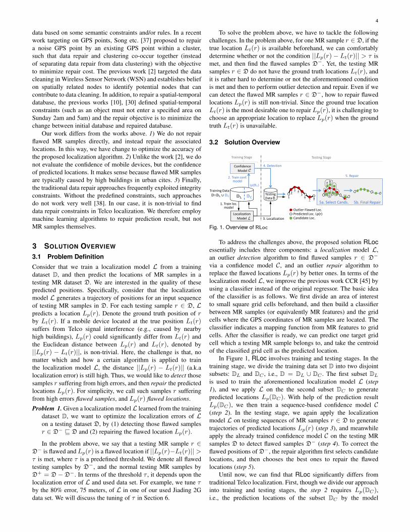
Fig. 1. Overview of RLoc

To address the challenges above, the proposed solution RLocessentially includes three components: a localization model L,an outlier detection algorithm to find flawed samples r ∈ D−

via a confidence model C, and an outlier repair algorithm toreplace the flawed locations Lp(r) by better ones. In terms of thelocalization model L, we improve the previous work CCR [45] byusing a classifier instead of the original regressor. The basic ideaof the classifier is as follows. We first divide an area of interestto small square grid cells beforehand, and then build a classifierbetween MR samples (or equivalently MR features) and the gridcells where the GPS coordinates of MR samples are located. Theclassifier indicates a mapping function from MR features to gridcells. After the classifier is ready, we can predict one target gridcell which a testing MR sample belongs to, and take the centroidof the classified grid cell as the predicted location.

In Figure 1, RLoc involves training and testing stages. In thetraining stage, we divide the training data set D into two disjointsubsets: DL and DC , i.e., D = DL ∪ DC . The first subset DLis used to train the aforementioned localization model L (step1), and we apply L on the the second subset DC to generatepredicted locations Lp(DC). With help of the prediction resultLp(DC), we then train a sequence-based confidence model C(step 2). In the testing stage, we again apply the localizationmodel L on testing sequences of MR samples r ∈ D to generatetrajectories of predicted locations Lp(r) (step 3), and meanwhileapply the already trained confidence model C on the testing MRsamples D to detect flawed samples D− (step 4). To correct theflawed positions of D−, the repair algorithm first selects candidatelocations, and then chooses the best ones to repair the flawedlocations (step 5).

Until now, we can find that RLoc significantly differs fromtraditional Telco localization. First, though we divide our approachinto training and testing stages, the step 2 requires Lp(DC),i.e., the prediction locations of the subset DC by the model

5

L. We then exploit the prediction locations Lp(DC) to acquirethe labels of confidence levels, which are next used to train theconfidence model C and finally to perform outlier detection andrepair. Thus, we can intuitively treat the confidence-model-basedoutlier detection and repair (i.e., steps 2, 4, 5 in Figure 1) as apost-processing phase of traditional Telco localization. Second, interms of the outlier detection and repair, the previous works suchas CRL (Confidence model-based data Repairing technique forTelco Localization) [43], employ single-point-based detection andrepair algorithms and do not take into account the connectivityof neighbouring locations. Instead, we adopt sequential detectionand repair algorithms for better results. Finally, to guarantee thefairness between our approach and other competitors, we still useD as the overall training dataset for the localization, detection andrepair algorithms in RLoc, and D as the testing dataset, with noextra training MR samples.

In the following Sections 4 and 5, we present the proposeddetection and repair algorithms, respectively. Moreover, if withoutspecial mention, we by default say that the proposed detec-tion/repair models are all sequence-based and MR samples havebeen re-processed to be sequence data.

4 CONFIDENCE-BASED DETECTION APPROACH

In this section, we first introduce the confidence level (Section4.1), and then present a sequence-based outlier detection algorithmvia the proposed confidence model (Section 4.2).

4.1 Confidence LevelWe define the confidence level by a binary indicator. If theconfidence level of a MR sample r ∈ D is 0, the sample r isflawed and otherwise normal.Definition 1. For a MR sample r and a localization model L, if

the distance ||Lp(r) − Lt(r)|| between a prediction locationLp(r) and ground truth Lt(r) is greater than a predefinedthreshold τ , i.e., ||Lp(r) − Lt(r)|| > τ , then we say thatr is a flawed sample and the confidence level of r is 0, andotherwise a normal sample with the confidence level 1.

To predict the confidence level of a testing sample r, our gen-eral idea is to learn a machine-learning-based confidence modelthat maps from training MR samples to the corresponding labelsof confidence levels. Unfortunately, the original training dataset Donly contains MR samples and GPS positions, but not confidencelevels. To this end, we give the following steps to find the labelsof confidence levels for training samples. Recall that we use thetwo disjoint subsets DL and DC to train a localization model Land a confidence model C, respectively (see Figure 1). After thelocalization model L is trained by DL, we then apply L on thesubset DC to predict the locations Lp(r) for the sample r ∈ DC .Since DC is still a training data subset, the sample r ∈ DC hasthe ground truth position Lt(r). We then follow Definition 1 tocompute the confidence level for every sample r ∈ DC . Once theconfidence level is available, we train a machine-learning-basedconfidence model C from these samples r ∈ DC to correspondingconfidence levels. After that, we apply the trained model C ontesting samples D to detect flawed ones D−.

In terms of the specific machine learning algorithm used totrain the confidence model C, a simple approach is to exploita binary-classifier such as Random Forest or GBDT (GradientBoosting Decision Tree) [1] to learn the mapping function from

an individual sample r ∈ DC to its confidence level. Note that it isstraightforward to extend our binary confidence levels to a multi-level confidence model (e.g., using the levels from 1 to 5). Forexample, we could leverage a multi-classifier, instead of a binaryclassifier, to support the multi-level confidence model.

Nevertheless, the approach above does not take into accountthe underlying spatio-temporal locality in neighbouring MR sam-ples, and is still inaccurate. In the rest of this section, to capturethe underlying spatio-temporal locality in neighbouring samples,we estimate the confidence levels of MR sequences for higheraccuracy first via a static HMM confidence model and then via animproved one, namely DA-HMM.

4.2 Static HMM-based Confidence ModelIn this section, we train a static HMM-based confidence modelC to learn the mapping between each MR sequence in DC and asequence of confidence levels by the following intuition.

Let us consider the scenario: a mobile device is moving firstclose to a certain serving base station (say bs) and then far awayfrom bs, until the device is with another serving base station.In this scenario, the mobile device generates a sequence of MRsamples. The signal strength of bs within such MR samplesbecomes first stronger and later weaker. If we treat the signalstrength ss (e.g., RSSI) of bs in MR samples as observation andthe confidence level as state, then the states (i.e., confidence levels)first become greater (i.e., one) and next smaller (i.e., zero).

When given an observed sequence of MR samples (containingbs and ss), we expect to infer a corresponding sequence of confi-dence levels via the following HMM decoding problem: given theparameters of HMM (acquired from the training data DC ) and theMR observation sequence for the testing dataset D, we aim to findthe most likely sequence of states (confidence levels). Formally,we describe the static HMM λ = (S, V,A,B, π) as follows.• S = 0, 1 is the set of states (confidence levels).• V = v1, ..., vk, ..., vM is the set of observations vk =〈vbsk , vssk 〉, where vbsk is a list of up to 7 base stations bsand vssk is the list of associated ss. Moreover, we convert thecontinuous readings of ss into 8 discrete levels: ss within therange [−50,−110] is converted to 6 levels from 2, 3,..., to 7by the equal interval of length 10, ss < −50 and ss > −110to the levels of 1 and 8, respectively.

• A = aij is the distribution of state transition probabilityaij of going from the confidence level i at time step t to thenext confidence level j at time step t+ 1.

• B = bj(k) is the distribution of emission probabilitybj(k) of observation vk in state j.

• π = πi is the initial state distribution with πi = P [q1 = Si].

4.3 A Dual-Stage Adaptive HMMThe static HMM model above may not work well on real MRsamples: the neighbouring MR samples within real sequence datafrequently exhibit uncertain timestamp intervals, e.g., caused byvarious sampling rate and data missing. Thus, besides the statessi and sj , the state transition probability aij further depends uponthe timestamp intervals between neighbouring MR samples. More-over, due to the high cost of collecting training samples, it is notrare that some areas of interest suffer from insufficient samples,leading to inaccurate estimation of the emission probability bj(k).

To address the issues above, we propose a dual-stage adaptiveHMM, named DA-HMM, on top of the static HMM model.

6

Specifically, after a static HMM model is learned by the samplesDC , in the training phase of DA-HMM, we introduce the timeinterval ∆ between neighbouring MR samples and the samplesize γ for observation k in state j, and define the new transitionprobability a∆

ij and emission probability bγj (k), respectively. Thenew probabilities are then adaptive to ∆ and γ. The detail toestimate a∆

ij and bγj (k) is as follows.

4.3.1 Adaptive State Transition Probability

0 25 50 75 100 125Time Interval Δ Δsecond)

0.00

0.05

0.10

0.15

0.20

0.25

0.30

Ratio

Jiading 2G Data

0 25 50 75 100 125Time In erval Δ Δsecond)

0.75

0.80

0.85

0.90

0.95

S a

e Tr

ansi

ion

Prob

abili

y

Jiading 2G Da aaΔ

1, 1

aΔ0, 1

0 25 50 75 100 125Time Inter al Δ Δsecond)

15

20

25

30

35

40

45

Localization Med

ain Error Δmeters) Jiading 2G Data

O erall Median Error

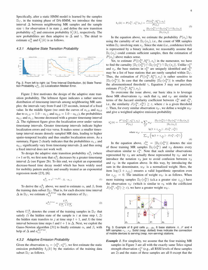
Fig. 2. From left to right: (a) Time Interval Distribution, (b) State Transi-tion Probability a∆

i,1, (c) Localization Median Error.

Figure 2 first motivates the design of the adaptive state tran-sition probability. The leftmost figure indicates a rather unevendistribution of timestamp intervals among neighbouring MR sam-ples: the intervals vary from 0 and 125 seconds, instead of a fixedvalue. In the middle figure (we omit the curves of a1,0 and a0,0

due to a1,0 = 1.0−a1,1 and a0,0 = 1.0−a0,1), the probabilitiesa0,1 and a1,1 become decreased with a greater timestamp interval∆. The rightmost figure gives the localization error under varioustimestamp intervals. Greater timestamp intervals indicate higherlocalization errors and vice versa. It makes sense: a smaller times-tamp interval means densely sampled MR data, leading to higherspatio-temporal locality and thus smaller localization errors. As asummary, Figure 2 clearly indicates that the probabilities a1,1 anda0,1 significantly vary from timestamp intervals ∆ and thus usinga fixed interval does not work well.

To design the adaptive state transition probability a∆i,1 (where

i = 1 or 0), we first note that a∆i,1 decreases by a greater timestamp

interval ∆ (see Figure 2b). To this end, we exploit an exponentialdecrease-based time decay model which has been widely usedfor mobility pattern analytic and usually treated as an exponentialregression mode [23], [6].

a∆i,1 = e

(−αi∆) · βi · ai,1 (1)

To derive the a∆i,1 above, we need to estimate αi and βi from

the training data subset DC . That is, for each discrete time interval∆ in DC , we estimate a∆,true

i,1 via the statistics of DC .

a∆,truei,1 =

U∆i,1

U∆i,1 + U∆

i,0

(2)

where U∆i,j denotes the count of the training samples in DC that

satisfy 1) the hidden state of the sample is i at time step t, 2)the hidden state transfers to j at time step t + 1, and 3) the timeinterval between time steps t and t+ 1 is ∆. Next, we exploit theGauss-Newton algorithm [31] to finally estimate αi and βi withhelp of ∆ and a∆,true

i,1 .

4.3.2 Adaptive Emission Probability

Given the observation vk = 〈vbsk , vssk 〉, we first estimate the staticemission probability bj(k) by the statistics of the training datasubset DC as follows.

bj(k) = P (vbsk , v

ssk |sj) =

P ((vbsk , bssk ), sj)

P (sj)

≈|DC(vbsk ) ∩ DC(vssk ) ∩ DC(sj)|

|DC(sj)|

(3)

In the equation above, we estimate the probability P (sj) byusing the carnality of set DC(sj), i.e., the count of MR sampleswithin DC involving state sj . Since the state (i.e., confidence level)is represented by a binary indicator, we reasonably assume thatDC(sj) could contain sufficient samples, then the estimation ofP (sj) above makes sense.

Yet, to estimate P ((vbsk , bssk ), sj) in the numerator, we have

to find the carnality |DC(vbsk ) ∩ DC(vssk ) ∩ DC(sj)|. Unlike vsskand sj , the base stations in vbsk are uniquely identified and vbskmay be a list of base stations that are rarely sampled within DC .Thus, the estimation of P ((vbsk , b

ssk ), sj) is rather sensitive to

|DC(vbsk )|. In case that the carnality |DC(vbsk )| is smaller thanthe aforementioned threshold γ, Equation 3 may not preciselyestimate P ((vbsk , b

ssk ), sj).

To overcome the issue above, our basic idea is to leveragethose MR observations vk′ such that vk and vk′ are similar interms of the Jaccard similarity coefficient between vbsk′ and vbsk ,i.e., the similarity J(vbsk , v

bsk′ ) ≥ ε, where ε is a given threshold

ε. Then, for every similar observation vk′ , we define a weight wk′and give a weighted adaptive emission probability

bγk(k) =

Pγ((vbsk , vssk ), sj)

P (sj)≈∑k′wk′ ·

|DC(vbsk′ ) ∩ DC(vssk ∩ DC(sj)||DC(sj)|

where wk′ =

lg(1 + zvbsk′

) · J(vbsk , vbsk′ )∑

vd

(lg(1 + z

vbsd

) · J(vbsk , vbsd )

)(4)

In the equation above, zbsvk = |DC(vbsk )| denotes the sizeof those training MR samples DC(vbsk ) and vd denotes everyobservation similar to vbsk . Note that such similar observationsrepresented by vd are actually those represented by vk′ and weintroduce the notation vd just to avoid confusion between vdand vk′ in the equation above. In this way, by introducing thesum in the denominator, wk′ is a normalized weight. Here, theitem log (1 + zvbs

k′) ensures a valid logarithmic operation even

for zvbsk′

= 0. The intuition of weight wk′ is as follows. Whenmore training samples DC(vbsk′ ) (a.k.a a greater size zvbs

k′) have

the observation vk′ (which is similar to vk with the coefficientJ(vbsk , v

bsk′ ) ≥ ε), we have a greater weight wk′ .

B

EFC

A

𝑟𝑟𝑑𝑑

𝑟𝑟𝑏𝑏

𝑟𝑟𝑎𝑎

𝑔𝑔1 𝑔𝑔2 𝑔𝑔3 𝑔𝑔4

𝑔𝑔5 𝑔𝑔6 𝑔𝑔7 𝑔𝑔8

𝑟𝑟𝑐𝑐

D

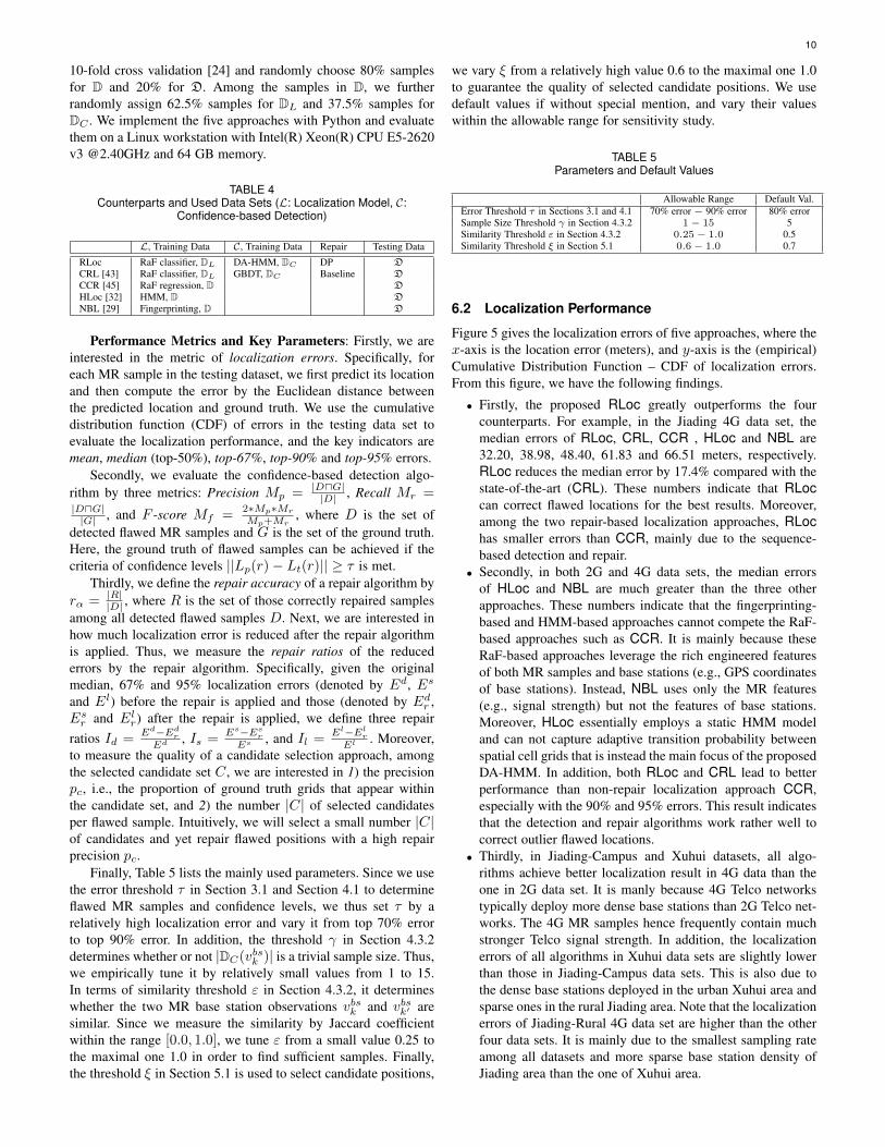
Fig. 3. Example of 8 grid cells g1...g8, 6 base stations A...F and 4MR samples ra...rd. Solid (resp. dotted) lines indicate the connectionof mobile devices to serving (resp. non-serving) stations.

Example 1. For simplicity, we assume that the four training MRsamples in Figure 3 are all with the exactly same Telco signalstrength observation vssk (e.g., all RSSI levels of these samplesare 2) and the states of these samples are all 0 except that the

7

state of rc is 1. Thus, we directly remove the subitems withrespect to vssk in the estimation of the emission probability (seeEquations 3 and 4).Suppose that we have the thresholds γ = 2 and ε = 0.5and need to estimate the emission probability bj(k) forsj = 0 and vbsk = B,E, F. Since no sample is withsuch sj and vbsk , we could follow Equation 3 and estimatethe static emission probability by zero. Nevertheless, thisestimation, which is sensitive to the sample size of DC(vbsk )with |DC(vbsk )| < γ = 2, may not make sense.Instead we follow Equation 4 to find two similar observationsvbsk′ : B,D,E in samples rb and rd, and B,E, F insample rc. Then for the first observation vbsk′ = B,D,E,we can compute the Jaccard similarity J(vbsk , v

bsk′ ) = 0.5 and

next wk′ = lg(2+1)·0.5lg(2+1)·0.5+lg(1+1)·1 = 0.44. For the second

observation vbsk′ = B,E, F, we compute wk′ = 0.56.Finally, we estimate bγj (k) = 0.44 · 2

3 + 0.56 · 03 = 0.293.

Recall that among the base stations within 4G LTE MRsamples collected by Android devices, only the serving stationis valid and other stations might be null (see Section 2.1).Then, to estimate the emission probability bj(k) for sj = 0and vbsk = B (differing from the above vbsk = B,E, F),we have |DC(vbsk )| = 3 > γ = 2 and then follow Equation 3to compute bγj (k) ≈ |DC(vbsk )∩DC(vssk )∩DC(sj)|

|DC(sj)| = 23 = 0.667.

To summarize the steps above, in Algorithm 1, we give thePseudo-code to estimate the parameters of DA-HMM. First, thelines 1-4 follow Section 4.3.1 to estimate the adaptive statetransition probability a∆

i,j , and lines 6-22 follow Section 4.3.2 toestimate the adaptive emission probability bγj (k).

Algorithm 1: Parameter Estimation in DA-HMMInput: Static HMM model λ = S, V,A,B, π, Training MR subset DC ,

Thresholds γ and εOutput: a∆

i,j and bγj (k)

1 Create a time interval list TList from nbr. samples within MR sequences inDC ;

2 foreach time interval δ ∈ TList do Infer aδ,truei,1 by the statistics of DC ;3 Estimate the parameters αa and βi in Eq. (1) with δ and aδ,truei,1 by

Gaussian-Newton method;4 Update a∆

i,1 ← e(−αi∆) · βi · ai,1 and a∆i,0 ← 1− a∆

i,1 ;5 foreach observation vk in V do6 Compute the sample size z

vbsk← |DC(vbsk )|;

7 if zvbsk≥ γ then Compute bγj (k) by Eq. (3);

8 else9 foreach similar observation vbs

k′ with J(vbsk , vbsk′ ) ≥ ε do

10 zbsk′ ← |Dc(v

bsk′ )|, and Compute wk′ by Eq. (4);

11 Computebγj (k) by Eq. (4);

12 return a∆i,j and bγj (k) ;

5 LOCATION REPAIR

Recall that the proposed confidence model can be applied ontoa testing sequence R = r1, ..., r|R| v D of MR samples todetect flawed samples. We are interested whether or not theseflawed samples are neighboring within the sequence R. Forexample, in Figure 1, we have detected five flawed samples withinan input sequence of 8 testing samples. Four of them (i.e., 2, ..., 5)are neighbouring within the input sequence and yet the one 7is disjoint from all other flawed samples. For a disjoint flawedsample, we find the most appropriate candidate location to replacethe flawed location Lp(r). Instead, to repair the neighboring

flawed locations, we then find the best sequence (a.k.a trajectory)of candidate locations. Since an individual flawed location can betreated as the special case of a sequence with the sequence lengthequal to 1, we thus generally focus on 1) finding the candidatelocations for every flawed location and 2) the repair of an entiresequence of neighboring flawed locations.

5.1 Candidate PositionsRecall that our multi-classifier-based localization model has al-ready divided an area of interest into multiple small grid cells.Thus, to find candidate positions, we alternatively select candidategrid cells. Before giving the detail, we first give the followingnotations. For a certain flawed sample r, the notation bsr indicatesthe set of those base stations appearing in r, and gr denotes thegrid cell where the position Lp(r) is located. For a grid cell g, thenotation BSg means the set of all base stations appearing in entireMR samples located within g.

With help of the notations above, we give the intuition offinding candidate positions. For a flawed sample r, a certain gridcell g becomes the candidate of gr , if the similarity of the two setsbsr and BSg is high and greater than a predefined threshold ξ.We measure the similarity as follows. Recall that bsr containsup to 6 or 7 base stations, i.e., |bsr| = 6 ∼ 7. Next, thegrid cell g may contain many MR samples and |BSg| is thuspossibly much greater than |bsr|. The standard Jaccard coefficientbetween bsr and BSg , which is very close to 0.0 no matterbsr, does not work well. Thus, we define a variant coefficientJ ′(bsr, BSg) =

|bsr⋂BSg|

|bsr| . Based on the intuition above, wethen give the following rule to find candidate grid cells for gr.

Gr = g ∈ G|J′(bsr, BSg) ≥ ξ (5)

where G denotes the set of all spatial grid cells in the area ofinterest, and ξ is a predefined threshold.Example 2. Still in Figure 3, we assume that rd is a flawed

sample and the threshold ξ = 0.5. For the grid cell g2

with the set BSg2 = A,B,D,E and g4 with the setBSg4 = B,E, F, we have J ′(bsrd , BSg2) = 1.0 andJ ′(bsrd , BSg4) = 2/3, both of which are greater than ξ. Wethus choose g2 and g4 as two candidates.

5.2 Sequence-based RepairWhen given a sequence of flawed locations Lp(r), the proposedrepair algorithm considers 1) the possibility or weight of a can-didate grid to repair every flawed location and 2) the transitionpossibility between two candidate grids, i.e., the possibility ofmobile devices to move from one candidate grid to the next one.To this end, we propose to maximize the joint probability of thepath to connect a sequence of candidate grids that are used torepair the entire sequence of flawed locations. Before giving thedefinition of the joint probability, we first define a repair graph.

Repair Graph: Consider a sequence R of N(= |R|) neigh-bouring flawed locations Lp(ri) with 1 ≤ i ≤ N . For each flawedlocation Lp(ri) and corresponding grid cell gri , we have a set Giof at most k candidate grids gi,j ∈ Gi with 1 ≤ j ≤ k. Formally,we define a repair graph G, where each vertex in G is mapped toa candidate grid gi,j . We build a directed edge from a candidatevertex gi,j to another vertex gi+1,j′ , if the corresponding locationsLp(ri) and Lp(ri+1) are neighbouring within the sequence R.Each vertex (and edge) is with an associated weight or probability(we will give the probability soon). Given the graph G, we have at

8

most kN paths from the source to sink. Among all such paths, wewant to find one path which is with the maximal joint probabilityto repair the N flawed locations.

Definition 2 (Vertex Weight). For a flawed location Lp(ri), wedefine the vertex weight Wgi,j of a candidate grid gi,j tomeasure the goodness of gi,j to repair Lp(ri).

For a non-flawed sample ri, no candidate grid is needed andwe simply set the vertex weight of gri by 1.0. For a flawed locationLp(ri) and a candidate gi,j , we compute the vertex weight Wgi,j

by the following equation.

Wgi,j=J′(bsri , BSgi,j ) · P (gi,j |BSgi,j ) · exp(−D(bs1ri

, BS1gi,j

))∑g∈Gri

J′(bsri , BSg) · P (g|BSg) · exp(−D(bs1ri, BS1

g))

In the equation above, we compute three sub-items.• J ′(bsri , BSgi,j ): the similarity coefficient between the

flawed MR ri and candidate grid cell gi,j in terms of theirbase stations.

• P (gi,j |BSgi,j ): the posterior probability.• D(bs1

ri , BS1gi,j ): the average physical distance between the

serving base station bsri in MR sample ri and those serv-ing stations of MR samples within gi,j . Since the servingbase station plays a key role in Telco localization, we thusintroduce D(·) to compute Wgi,j .

D(bs1ri, BS

1gi,j

) =

0, bs1ri

∈ BS1gi,j∑

bs∈BS1gi,j

d(bs1r,i,bs)

|BS1gi,j|

, otherwise

where d(·) denotes the Euclidean distance between the twobase stations. Thus, D(bs1

ri , BS1gi,j ) indicates the average

distance between the serving base station bsri and eachserving station within the grid gi,j .

Besides the vertex weight in a repair graph G, we also considerthe transition possibility of mobile devices to move from oneposition to the next one. Thus, we define the following transitionprobability as the edge weight.

Definition 3 (Edge Weight). For a directed edge gi,j → gi+1,j′

from a candidate grid gi,j to the next one gi+1,j′ within a pathof the repair graph G. The edge weight is computed as follows.

Wgi,j→gi+1,j′∝

cos θ

d(gi,j , gi+1,j′ )(6)

In the equation above, d(gi,j , gi+1,j′) is the Euclidean dis-tance between gi,j and gi+1,j′ , and θ is the angle between thetwo edges gi−1,j′′ → gi,j and gi,j → gi+1,j′ . The intuition tocompute the edge weight Wgi,j→gi+1,j′ is as follows. Whenone mobile device is walking or driving on a road, it is notlikely to change the direction very frequently, and the physicaldistance between two neighbouring vertices (i.e., two neighboringlocations) should not be very far away.

Example 3. Figure 4 illustrates an example repair graph G, wherethe source and sink are normal. For the two flawed locationsLp(ri) and Lp(ri+1), we have 3 candidate grids gi,1, gi,2, gi,3and 2 candidate grids gi+1,1, gi+1,2, respectively, and thustotally have 6 paths from source gri−1

to sink gri+2. Among

the six paths, we choose one path with the maximal jointprobability. The candidate grids within the selected path arethen used to repair the flawed locations Lp(ri) and Lp(ri+1),

Source Sink

Fig. 4. Example of a Repair Graph and Illustration of three angles: θ1between the edges Lp(ri−1)→ gi,1 and gi,1 → gi+1,1, θ2 between theedges Lp(ri−1) → gi,2 and gi,2 → gi+1,1, and θ3 between the edgesLp(ri−1)→ gi,3 and gi,3 → gi+1,1

respectively. In addition, this figure gives an example of threeangles θ1, θ2 and θ3 between repair graph edges.

Until now, in the repair graph G, each vertex gi,j is with aweight Wgi,j and each edge gi,j → gi+1,j′ is with a weightWgi,j→gi+1,j′ . Our task is to find a path from the source tosink, such that the found path is with the largest joint probability.Consider a path ω = g1 → ... → g|ω| that traverses |ω| verticesfrom g1 to g|ω|, we compute the joint probability of ω.

P (ω) = Wg1·Wg1→g2 ·Wg2

...Wg|Ω|−1·Wg|Ω|−1→g|Ω| ·Wg|ω| (7)

5.3 Algorithm Detail

Algorithm 2: DP-based Repair AlgorithmInput: G Repair Graph, Gvertex(·) vertex weight, Gedge(·) edge weightOutput: rSeq the path with the max. joint probability

1 JP []← the highest joint probability so far;2 par[]← parent nodes of current candidates;3 Vparent ← those vertices in G without parents;4 foreach vp ∈ Vparent do JP [vp]← Gvertex(vp) ;5 while Vparent still has children in G do6 max=−∞, Vchild ← child vertices of Vparent in G;7 foreach vc ∈ Vchild do8 foreach vp ∈ Vparent do9 if |Vchild| == 1 then tmp=JP [vp] ;

10 else tmp=JP [vp]× Gvertex(vp)× Gedge(vp→ vc) ;11 if tmp > max then max = tmp; par[vc] = vp ;12 JP [vc]=max;

13 Vparent ← Vchild;

14 Initialize rSeq as an empty list;15 c=argMaxv(JP [v]), add R to rSeq;16 while par[c] 6= ∅ do add par[c] to rSeq, c← par[c] ;17 return rSeq;

Algorithm 2 outlines the sequence-based repair via a dynamicprogramming method. It requires an input repair graph G andgenerates a trajectory or equivalently a path of selected candidatepositions having the maximal joint probability. In general, findingsuch a path in a repair graph is NP-hard. Thus, we design an ef-ficient path planning algorithm. The planning algorithm first findsthe vertices Vparent having no parent (line 3) after the initiationof two variables JP [] (joint probability) and par[] in lines 1-2.Next, the loop in lines 5-13 visits the remaining vertices level bylevel in the repair graph G by a Breadth-First Search (BFS) style.The JP [] maintains the largest joint probabilities from sink to thecurrent vertices so far. Thus, when the edges from vp ∈ Vparentto vc ∈ Vchild are considered, we are interested in the maximaljoint probability JP [vp]×Gvertex(vp)×Gedge(vp→ vc), where

9

Gvertex(vp) denotes the vertex weight of vp and Gedge(vp→ vc)denotes the weight of the edge vp → vc. Such maximal productis again maintained by a new item JP [vp]. Meanwhile the itempar[vc] with respect to vc maintains the parent vertex vp. OnceVparent has no child, the entire graph G has been visited and thesink has been reached. Thus, the algorithm breaks the loop. Nowwe simply find the item v in JP [] leading to the maximal JP [v](line 15). By reversely tracking the parent par[c] of such founditem v (line 16), we can return a sequence of desirable candidatesleading to the maximal JP [v].

The running time of Algorithm 2 heavily depends upon thepath planning, especially the two loops in lines 8-13. Suppose therepair graph G has n neighbouring flawed locations, i.e., n levelsfrom source to sink, and each level has k candidates. Thus, therunning time of the path planning part is O(kn). Note that theprevious work [28] does not adopt any detection algorithm. Thus,when given an entire sequence of continuous grids (no matterflawed or not), the running time of [28] is O(kN ), where N isthe size of the entire sequence. Thus, our repair algorithm cansignificantly improve the efficiency from O(kN ) to O(kn) inparticular due to N n.

6 EVALUATION

In this section, we evaluate our approach RLoc in terms of threeaspects: the overall localization accuracy after RLoc is appliedto correct flawed positions, the performance of the proposeddetection and repair algorithms, and sensitivity study of RLocto key parameters.

6.1 Experimental SettingData sets: In Table 3, we use totally three datasets: two collectedfrom the rural Jiading district of North-west Shanghai, and onefrom the urban Xuhui district in the core center Shanghai (Thephysical distance between the two districts is around 31 km).

TABLE 3Statistics of Used Data Sets

Jiading-Campus Xuhui Jiading-Rural2G 4G 2G 4G 4G

Num. of IMSIs 7 4 4 3 5967Num. of samples 20324 14218 24570 16905 150288Sampling Period (sec) 2∼3 2∼3 1 1 10∼11Density of Serving Stations 25.85 29.43 28.18 38.76 24.92Num. of Serving Stations 61 44 21 16 508Coverage Area (km2) 1.64*1.44 1.32*0.43 4.46*4.57

• Jiading-Campus: This dataset, collected by our developedAndroid App, contains MR samples collected from 2G GSMand 4G LTE networks in a university campus that is locatedwithin the rural Jiading area. When students holding mobiledevices installed with the App are moving around outdoorcampus roads, the App then collects MR samples and currentGPS coordinates. Table 2 shows the data format of thisdataset. Note that, probably due to the limitation of AndroidAPI and policy rules of backend system configuration withrespect to Telco networks, the identifiers (RNCID 2∼7 andCellID 2∼7) of non-serving base stations are null values,though the associated RSSI measurements could be collectedin 4G MR samples.

• Xuhui: This dataset contains 2G and 4G samples collectedon several main roads. As mentioned in Section 2.1, the

data formats of MR samples collected by frontend AndroidAPIs and backend operators may differ. For example, thebackend 2G samples contain the signal measurements suchas RxLev (= RSSI), ARFCN (absolute radio-frequency chan-nel number) and the backend 4G MR samples contain theidentifiers of all connected base stations and the associatedsignal measurements such as RSSI, RSRP and RSRQ. Thedetail of these data formats refer to the previous work [20].

• Jiading-Rural: This large dataset contains 4G LTE MR sam-ples collected in a large rural area in Jiading. The samplingrate of this dataset is rather low, i.e., one sample for every10∼11 seconds, when compared with other datasets. Thisdataset follows the same data format as Xuhui dataset.

Similar to the previous works NBL [29] and CCR [45], weuse GPS coordinates as the ground truth locations of MR samples.Since the collected GPS coordinates may contain noisy informa-tion, we exploit the map-matching technique [19] to mitigate theeffect of noisy information. To protect user privacy, all IMSIs(International Mobile Subscriber Identity) in the used datasetshave been anonymized.

Counterparts and Data Division: In Table 4, we evaluateRLoc against four counterparts, including three outdoor localiza-tion approaches: a Random Forest regressor-based approach CCR[45], HMM-based localization approach [32] (for simplicity werename this HMM-based approach as HLoc), and fingerprinting-based localization approach NBL [29]) and our previous datarepair-based approach CRL [43]. Note that HLoc [32] originallyworks only on 4G LTE data and requires the items of bothTA (Timing Advance) and RSRP (Reference Signal ReceivingPower). Since the MR samples in our used datasets do not containthe TA item and the MR samples in 2G datasets or frontendAndroid datasets do not contain the RSRP item, for fairness, ourimplementation of [32] has to remove the component regardingTA and then replace RSRP by RSSI.

These five approaches all require localization steps, and onlytwo of them RLoc and CRL [43] require the localization, detectionand repair steps. Here, both RLoc and CRL [43] use a RaFclassifier-based localization model L, whereas CCR [45] adoptsa RaF regressor-based localization model. The input to the threeRaf-based localization algorithms contain the features such as rawMR features (see Table 2), base station features (e.g., GPS coor-dinates of base stations) provided by Telco operators, and hand-made contextual features (e.g., the moving speed and direction[45]). Nevertheless, RLoc and CRL differ in terms of the useddetection and repair algorithms: RLoc exploits the sequenced-based approach, and yet CRL the single-point-based approach.

We give the training and testing data of the five approaches asfollows. CCR, HLoc and NBL do not require detection and repairalgorithms. We thus assign the entire datasets D and D to train andtest a localization model for them, respectively. Instead, besidesthe localization model L, RLoc and CRL require detection andrepair algorithms. Thus, we assign the subset DL as the trainingdataset for L and the subset DC as the training data for the detec-tion/repair algorithms. In this way, the same training dataset D isassigned to all five approaches, and we do not assign extra moresamples to train the localization/detection/repair algorithms forRLoc and CRL. Thus, our data assignment guarantees evaluationfairness for five approaches.

For the proportion of MR samples assigned for DL, DC , andD, we divide the samples in each MR dataset into three disjointparts (see Table 4). Specifically, to avoid over-fitting, we adopt the

10

10-fold cross validation [24] and randomly choose 80% samplesfor D and 20% for D. Among the samples in D, we furtherrandomly assign 62.5% samples for DL and 37.5% samples forDC . We implement the five approaches with Python and evaluatethem on a Linux workstation with Intel(R) Xeon(R) CPU E5-2620v3 @2.40GHz and 64 GB memory.

TABLE 4Counterparts and Used Data Sets (L: Localization Model, C:

Confidence-based Detection)

L, Training Data C, Training Data Repair Testing Data

RLoc RaF classifier, DL DA-HMM, DC DP DCRL [43] RaF classifier, DL GBDT, DC Baseline DCCR [45] RaF regression, D DHLoc [32] HMM, D DNBL [29] Fingerprinting, D D

Performance Metrics and Key Parameters: Firstly, we areinterested in the metric of localization errors. Specifically, foreach MR sample in the testing dataset, we first predict its locationand then compute the error by the Euclidean distance betweenthe predicted location and ground truth. We use the cumulativedistribution function (CDF) of errors in the testing data set toevaluate the localization performance, and the key indicators aremean, median (top-50%), top-67%, top-90% and top-95% errors.

Secondly, we evaluate the confidence-based detection algo-rithm by three metrics: Precision Mp = |DuG|

|D| , Recall Mr =|DuG||G| , and F -score Mf =

2∗Mp∗Mr

Mp+Mr, where D is the set of

detected flawed MR samples and G is the set of the ground truth.Here, the ground truth of flawed samples can be achieved if thecriteria of confidence levels ||Lp(r)− Lt(r)|| ≥ τ is met.

Thirdly, we define the repair accuracy of a repair algorithm byrα = |R|

|D| , where R is the set of those correctly repaired samplesamong all detected flawed samples D. Next, we are interested inhow much localization error is reduced after the repair algorithmis applied. Thus, we measure the repair ratios of the reducederrors by the repair algorithm. Specifically, given the originalmedian, 67% and 95% localization errors (denoted by Ed, Es

and El) before the repair is applied and those (denoted by Edr ,Esr and Elr) after the repair is applied, we define three repairratios Id =

Ed−EdrEd

, Is =Es−EsrEs , and Il =

El−ElrEl

. Moreover,to measure the quality of a candidate selection approach, amongthe selected candidate set C , we are interested in 1) the precisionpc, i.e., the proportion of ground truth grids that appear withinthe candidate set, and 2) the number |C| of selected candidatesper flawed sample. Intuitively, we will select a small number |C|of candidates and yet repair flawed positions with a high repairprecision pc.

Finally, Table 5 lists the mainly used parameters. Since we usethe error threshold τ in Section 3.1 and Section 4.1 to determineflawed MR samples and confidence levels, we thus set τ by arelatively high localization error and vary it from top 70% errorto top 90% error. In addition, the threshold γ in Section 4.3.2determines whether or not |DC(vbsk )| is a trivial sample size. Thus,we empirically tune it by relatively small values from 1 to 15.In terms of similarity threshold ε in Section 4.3.2, it determineswhether the two MR base station observations vbsk and vbsk′ aresimilar. Since we measure the similarity by Jaccard coefficientwithin the range [0.0, 1.0], we tune ε from a small value 0.25 tothe maximal one 1.0 in order to find sufficient samples. Finally,the threshold ξ in Section 5.1 is used to select candidate positions,

we vary ξ from a relatively high value 0.6 to the maximal one 1.0to guarantee the quality of selected candidate positions. We usedefault values if without special mention, and vary their valueswithin the allowable range for sensitivity study.

TABLE 5Parameters and Default Values

Allowable Range Default Val.Error Threshold τ in Sections 3.1 and 4.1 70% error − 90% error 80% errorSample Size Threshold γ in Section 4.3.2 1− 15 5Similarity Threshold ε in Section 4.3.2 0.25− 1.0 0.5Similarity Threshold ξ in Section 5.1 0.6− 1.0 0.7

6.2 Localization Performance

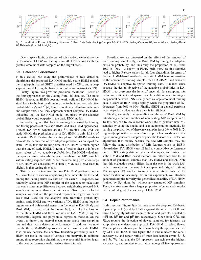
Figure 5 gives the localization errors of five approaches, where thex-axis is the location error (meters), and y-axis is the (empirical)Cumulative Distribution Function – CDF of localization errors.From this figure, we have the following findings.

• Firstly, the proposed RLoc greatly outperforms the fourcounterparts. For example, in the Jiading 4G data set, themedian errors of RLoc, CRL, CCR , HLoc and NBL are32.20, 38.98, 48.40, 61.83 and 66.51 meters, respectively.RLoc reduces the median error by 17.4% compared with thestate-of-the-art (CRL). These numbers indicate that RLoccan correct flawed locations for the best results. Moreover,among the two repair-based localization approaches, RLochas smaller errors than CCR, mainly due to the sequence-based detection and repair.

• Secondly, in both 2G and 4G data sets, the median errorsof HLoc and NBL are much greater than the three otherapproaches. These numbers indicate that the fingerprinting-based and HMM-based approaches cannot compete the RaF-based approaches such as CCR. It is mainly because theseRaF-based approaches leverage the rich engineered featuresof both MR samples and base stations (e.g., GPS coordinatesof base stations). Instead, NBL uses only the MR features(e.g., signal strength) but not the features of base stations.Moreover, HLoc essentially employs a static HMM modeland can not capture adaptive transition probability betweenspatial cell grids that is instead the main focus of the proposedDA-HMM. In addition, both RLoc and CRL lead to betterperformance than non-repair localization approach CCR,especially with the 90% and 95% errors. This result indicatesthat the detection and repair algorithms work rather well tocorrect outlier flawed locations.

• Thirdly, in Jiading-Campus and Xuhui datasets, all algo-rithms achieve better localization result in 4G data than theone in 2G data set. It is manly because 4G Telco networkstypically deploy more dense base stations than 2G Telco net-works. The 4G MR samples hence frequently contain muchstronger Telco signal strength. In addition, the localizationerrors of all algorithms in Xuhui data sets are slightly lowerthan those in Jiading-Campus data sets. This is also due tothe dense base stations deployed in the urban Xuhui area andsparse ones in the rural Jiading area. Note that the localizationerrors of Jiading-Rural 4G data set are higher than the otherfour data sets. It is mainly due to the smallest sampling rateamong all datasets and more sparse base station density ofJiading area than the one of Xuhui area.

11

0 20 40 60 80 100 120 140Error (meters)

0.20

0.50

0.67

0.900.95

CDF

Jiading-Campus 2G Data

RLocCRLCCRHLocNBL

0 20 40 60 80 100 120 140Error (meters)

0.20

0.50

0.67

0.900.95

CDF

Xuhui 2G Data

RLocCRLCCRHLocNBL

0 20 40 60 80 100 120 140Error (meters)

0.20

0.50

0.67

0.900.95

CDF

Jiading-Campus 4G Data

RLocCRLCCRHLocNBL

0 20 40 60 80 100 120 140Error (meters)

0.20

0.50

0.67

0.900.95

CDF

Xuhui 4G Data

RLocCRLCCRHLocNBL

0 25 50 75 100 125 150 175 200Error (meters)

0.20

0.50

0.67

0.900.95

CDF

Jiading-Rural 4G Data

RLocCRLCCRHLocNBL

Fig. 5. Localization Errors of Five Algorithms on 5 Used Data Sets: Jiading-Campus 2G, Xuhui 2G, Jiading-Campus 4G, Xuhui 4G and Jiading-Rural4G Datasets (from left to right).

Due to space limit, in the rest of this section, we evaluate theperformance of RLoc on Jiading-Rural 4G LTE dataset (with thegreatest amount of data samples on the largest area).

6.3 Detection PerformanceIn this section, we study the performance of four detectionalgorithms: the proposed DA-HMM model, static HMM model,the single-point-based GBDT classifier used by CRL, and a deepsequence model using the basic recurrent neural network (RNN).

Firstly, Figure 6(a) gives the precision, recall and F-score ofthe four approaches on the Jiading-Rural 4G data set. The staticHMM (denoted as HMM) does not work well, and DA-HMM in-stead leads to the best result mainly due to the introduced adaptiveprobabilities a∆

i,j and bγj (k) to incorporate uncertain time-intervalsand sample size. The RNN approach cannot compete DA-HMM,indicating that the DA-HMM model optimized by the adaptiveprobabilities could outperform the basic RNN model.

Secondly, Figure 6(b) plots the running time (used by trainingand testing phases) of the static HMM and DA-HMM approaches.Though DA-HMM requires around 3× training time over thestatic HMM, the prediction time of DA-HMM is only 1.18× ofthe static HMM. During the training phase, DA-HMM needs toestimate the parameters of two adaptive probabilities on top of thestatic HMM, thus the training time of DA-HMM is much higherthan the one of static HMM. In terms of testing phase to infer theexact values of two adaptive probabilities, DA-HMM calculatesthe specific time intervals between neighbouring MR sampleswithin testing sequence data. Since the remaining prediction stepsof DA-HMM are consistent with static HMM, DA-HMM leads toslightly higher testing time cost.

Thirdly, we are interested in how DA-HMM performs on theMR samples with various neighboring time intervals. To this end,among the Jiading-Rural 4G data set, for each MR sequence, werandomly select some MR samples of the sequence to make surethat every timestamp difference between neighboring selected MRsamples is no more than a certain value. Given these selectedsamples, we evaluate the proposed exponential regression-basedDA-HMM (used for the adaptive state transition probability)against static HMM and two variants of DA-HMM using logisticregression and polynomial regression (denoted as DA-HMMl andDA-HMMp, respectively). In Figure 6(c), we plot the F-scoreof the static HMM and three variants of DA-HMM (using theexponential, logistic and polynomial regression models). On theoverall, a higher time interval means more sparse time samplingrate and thus worse detection performance. In addition, we notethat the three DA-HMM approaches outperform the static HMM.It is mainly because the adaptive transition probability in DA-HMM can tackle the issue of various time intervals. In addition,among three regression algorithms, the exponential function leadsto the best performance under various time intervals.

Fourthly, we are interested in the effect of the amount ofused training samples DC on DA-HMM by tuning the adaptiveemission probability, and thus vary the proportion of DC from10% to 100%. As shown in Figure 6(d), more training sampleslead to higher F-score values for all four algorithms. In terms ofthe two HMM-based methods, the static HMM is more sensitiveto the amount of training samples than DA-HMM, and whereasDA-HMM is adaptive to sparse training data. It makes sensebecause the design objective of the adaptive probabilities in DA-HMM is to overcome the issue of uncertain data sampling rateincluding sufficient and sparse data. In addition, since training adeep neural network RNN usually needs a large amount of trainingdata, F-score of RNN drops rapidly when the proportion of DCdecreases from 50% to 10%. Finally, GBDT in general performsworst especially when training data is insufficient.

Finally, we study the generalization ability of DA-HMM byintroducing a certain number of new testing MR samples in D.To this end, we follow a recent work [36] to generate new MRsamples by using the spatial and scan augmentation methods. Byvarying the proportion of these new samples from 0% to 50% in D,Figure 6(e) plots the F-scores of four approaches. As shown in thisfigure, more generated samples degrade the F-score of all detectionalgorithms. It is mainly because the new MR samples may notfollow the same distribution of MR features (such as RSSI).Nevertheless, DA-HMM can still lead to competitive performanceeven if 50% testing data are generated samples, and instead thestatic HMM and RNN-based methods are rather sensitive to theamount of generated samples than DA-HMM and GBDT. Notethat this evaluation result differs from the one in the work [36]which instead uses the new MR samples and original trainingMR samples (D) together to train a localization model L forbetter localization accuracy. Yet in our experiment, we introducegenerated samples to verify the generalization ability of DA-HMM(trained by DC alone, but without any generated MR samples).Thus, it makes sense that a larger proportion of generated samplesin D could degrade the accuracy of DA-HMM.

6.4 Repair Performance

In this section, Figure 7(a) first evaluates the proposed DP-basedrepair approach (used by RLoc) against the repair in CRL andthree filtering algorithms: mean, Kalman and particle, denoted asmFilter, kFilter and pFilter, respectively. Since both CRL andRLoc require the detection of flawed samples, for fairness, weadopt the same detection approach DA-HMM to select flawedMR samples and then repair these samples by the approaches usedby CRL and RLoc. In this figure, the x-axis indicates the repairaccuracy rα and repair ratios of three localization errors Id, Isand Il. We find that the DP approach can achieve the highestaccuracy rα and greatest repair ratios among all five approaches.

12

Precision Recall F-score0.0

0.2

0.4

0.6

0.8

1.0Jiading-Rural 4G Data

CRL(GBDT)HMMRNNDA-HMM

Training Prediction0

20

40

60

80

100

120

Running Time (second)

Jiading-Rural 4G DataHMMDA-HMM

10 25 50 75 100 125Time Interval (second)

0.2

0.3

0.4

0.5

0.6

0.7

0.8

Valu

e of

F-s

core

Jiading-Rural 4G Data

DA-HMMDA-HMMl

DA-HMMp

HMM

10 20 50 80 100Proportion (%) of Training Samples

0.2

0.3

0.4

0.5

0.6

0.7

0.8

Value of F-sco

re

Jiading-Rural 4G Data

DA-HMMCRL(GBDT)HMMRNN

0 10 20 30 40 50Proportion (%) of Generated MRs in Testing Data

0.2

0.3

0.4

0.5

0.6

0.7

0.8

Value of F-score

Jiading-Rural 4G Data

DA-HMMCRL(GBDT)HMMRNN

Fig. 6. Detection Algorithm: (a-b) Effectiveness and Efficiency of Detection Approaches, (c-e) Effect of Time Intervals, Used Training Samples, andGenerated MR samples in Testing Data (from left to right).

rα Id Is Il0.0

0.2

0.4

0.6

0.8

1.0

Accu

racy

& Im

provem

ent

Jiading-Rural 4G DataCRLmFliterkFliterpFliterRLoc(DP)

pc |C|0.5

0.6

0.7

0.8

0.9

1.0

Value of p

c

0

4

8

12

16

20

Value of |c|

Jiading-Rural 4G DataCRLRaFRLoc

Fig. 7. Repair Approach: Evaluation of Five Repair Approaches (left) andEffect of Candidate Selection approaches (right).

It is mainly because the DP approach repairs the entire sequenceof flawed MR samples.

Secondly, consider that the candidate set C is the key of arepair algorithm. Thus, we compare our approach against twoalternative candidate selection approaches: 1) CRL utilizes aprobability Matrix M to lookup candidates for a given flawedgrid, and 2) Random Forest (RaF) classification-based localizationmodel predicts the probability for each possible grid to be theposition grid of a testing MR sample. Such a probability can beused to select those top-k grids with the highest probabilities asthe candidate grids. In Figure 7(b), the left and right y-axis plotsthe repair precision pc and the number |C| of selected candidates(defined in § 6.1) of three repair approaches. CRL suffers fromthe lowest repair precision but selects the smallest candidate grids.Though the Random Forest (RaF) classifier can achieve betterresult than CRL, but at the cost of the most number of selectedcandidates (and thus high overhead to prune unneeded candidates).Finally, our approach can achieve the highest precision pc and themiddle amount of selected candidates per flawed sample, 10, ismuch smaller than the one by RaF. This experiment indicates thatour work can lead to the best trade-off between the repair precisionand overhead of selecting candidates.

70 75 80 85 90Error Threshold τ (×% error)

0.2

0.4

0.6

0.8

1.0

Precision & Recall &

F-score

Jiading-Rural 4G DataPrecision Recall F-score

1 3 5 8 12 15Sample Size Threshold γ

0.2

0.4

0.6

0.8

1.0

Prec

ision

& R

ecal

l & F

-sco

re

Jiading-Rural 4G DataPrecision Recall F-score

Fig. 8. Sensitivity Study: Effect of Error Threshold τ (left) and SampleSize Threshold γ (right).

6.5 Sensitive StudyIn this section, we vary the values of several key parameters andstudy the performance of RLoc.

Firstly, we are interested in how DA-HMM is sensitive to thethreshold τ which is used to determine the confidence levels to

detect flawed samples. Depending upon the errors of a localizationmodel L, we vary the threshold τ from top-70% error to top-90%error (and thus the threshold τ becomes greater), and measurethe performance of the detection algorithm. Figure 8(a) showsthe precision, recall and F-score of DA-HMM. When τ becomesgreater, the detection precision drops slightly. Nevertheless, witha larger τ , the recall first grows and later slightly drops. Forexample, the threshold τ = 80% error leads to the highest recall.Finally, the F-score unifies precision and recall, and exhibits thesimilar trend as the recall.

TABLE 6Effects of Two Thresholds ε and ξ.

SimilarityThreshold ε

Jiading-Rural 4G SimiliartyThreshold ξ

Jiading-Rural 4GMp Mr Mf rα pc |C|

0.25 0.833 0.601 0.698 0.6 0.651 0.907 12.30.50 0.863 0.603 0.710 0.7 0.686 0.901 9.90.75 0.859 0.582 0.694 0.8 0.690 0.875 8.21.0 0.852 0.574 0.686 1.0 0.694 0.842 6.7

Secondly, we study the effect of the threshold γ on our detec-tion algorithm. This threshold γ is to determine whether or not theset |DC(vbsk )| contains sufficient samples, i.e., |DC(vbsk )| ≥ γ,during the estimation of the adaptive emission probability. Byvarying γ from 1 to 15, we evaluate the detection performanceof DA-HMM. In Figure 8(b), the precision, recall and F-score ofDA-HMM grow until γ = 5 and then degrade slightly. It is mainlybecause too many observation samples are unnecessary to tune theadaptive probability due to the used sufficient training samples.Thus, we by default set γ by 5.

Thirdly, we study the effect of ε in the detection algorithm.Recall that in the DA-HMM detection algorithm, we adopt asimilarity threshold ε to determine whether or not two base stationobservations are similar. In Table 6, either a too small or toolarge threshold ε may not lead to the greatest performance. Here,ε = 0.5 helps achieving the best F-score.

Finally, we are interested in the effect of threshold ξ on ourrepair algorithm. In the repair algorithm, we use a similaritythreshold ξ to determine whether or not a certain spatial gridcell is a candidate. Table 6 shows the effect of ξ on the repairperformance. Firstly, a greater ξ leads to a smaller number |C| ofcandidates for each flawed MR sample and higher repair accuracyaα. Moreover, the repair precision pc decreases with a greater ξ.For example given ξ = 1.0, it means that among the up-to 7 basestations in a flawed MR sample, all of them are selected to be theobservation set of the candidates. Thus, to balance the precisionand number |C|, we by default set ξ = 0.7.

6.6 DiscussionTelco MR data usually contain privacy sensitive informationsuch as locations and IMSI information of individuals. Privacy

13

preservation techniques can be used to address the privacy issue.For example, we anonymized user identifiers (IMSI) in MRsamples. Moreover, we have replaced a real user ID with multiplevirtual ones, such that an entire trajectory of this real user couldbe divided into multiple disjoint sub-trajectories with respect tosuch virtual users. In this way, we avoid the exposure of anentire trajectory. Nevertheless, the introduced privacy preservationtechniques compromise localization accuracy. Our long-term goalis to adopt privacy techniques including differential privacy [18]to support privacy-preserving machine learning and accurate dataanalytics in big Telco MR data.

7 CONCLUSION

In this paper, we proposed a sequence-based localization frame-work to detect and repair outlier positions for lower Telco localiza-tion errors. First, the detection approach DA-HMM, via a binaryconfidence level, can overcome the issues of various time intervalsof neighbouring MR samples and uneven amount MR samplesacross base stations. Second, the repair approach leverages a repairgraph by incorporating the importance of each candidate andtransition between neighbouring candidates to choose a best pathwith the largest joint probability. The evaluation on three datasetsvalidates that our work greatly outperforms both the single-point-based and traditional sequence-based localization approaches, e.g.,those using static HMM models.

As future work, we continue to explore more advanced ma-chine learning techniques for Telco localization. For example therecent work [42] explored transferable knowledge from trainingdata set to testing data. Such success inspired us to potentially findtransferring knowledge between MR samples and GPS locations.

ACKNOWLEDGE

This research has been supported in part by National NaturalScience Foundation of China (Grant No. 61972286 and No.61772371), project 16214817 from the Research Grants Councilof Hong Kong and the 5GEAR project and FIT project from theAcademy of Finland. We also would like to thank anonymousreviewers for their valuable comments.

REFERENCES

[1] https://en.wikipedia.org/wiki/Gradient boosting.[2] Q. B. Ali, N. Pissinou, and K. Makki. Belief based data cleaning

for wireless sensor networks. Wireless Communications and MobileComputing, 12(5):406–419, 2012.

[3] H. Aly and M. Youssef. Dejavu: an accurate energy-efficient outdoorlocalization system. In SIGSPATIAL/GIS, pages 154–163. ACM, 2013.

[4] R. Arthi and K. Murugan. Localization in wireless sensor networksby hidden markov model. In International Conference on AdvancedComputing, pages 14–18, 2010.

[5] A. Asahara, K. Maruyama, A. Sato, and K. Seto. Pedestrian-movementprediction based on mixed markov-chain model. In GIS, pages 25–33.ACM, 2011.

[6] E. S. C. and P. Vega-Jorquera. Modelling temporal decay of aftershocksby a solution of the fractional reactive equation. Applied Mathematicsand Computation, 340:43–49, 2019.

[7] J. J. Caffery and G. L. Stuber. Overview of radiolocation in cdmasystems. IEEE Communications Magazine, 36(4):38–45, 1998.

[8] A. Chakraborty, L. E. Ortiz, and S. R. Das. Network-side positioning ofcellular-band devices with minimal effort. In 2015 IEEE Conference onComputer Communications (INFOCOM), pages 2767–2775, 2015.

[9] L. Cong and W. Zhuang. Hybrid TDOA/AOA mobile user location forwideband CDMA cellular systems. IEEE Trans. Wireless Communica-tions, 1(3):439–447, 2002.

[10] T. Emrich, H. Kriegel, M. Mauder, M. Renz, G. Trajcevski, and A. Zufle.Minimal spatio-temporal database repairs. In SIGSPATIAL/GIS, pages482–485. ACM, 2013.

[11] S. C. Ergen, H. S. Tetikol, M. Kontik, R. Sevlian, R. Rajagopal,and P. Varaiya. Rssi-fingerprinting-based mobile phone localizationwith route constraints. IEEE Transactions on Vehicular Technology,63(1):423–428, 2014.

[12] S. Gambs, M. Killijian, and M. N. del Prado Cortez. Show me how youmove and I will tell you who you are. volume 4, pages 103–126, 2011.

[13] S. Gambs, M.-O. Killijian, and M. N. n. del Prado Cortez. Next placeprediction using mobility markov chains. In Proceedings of the FirstWorkshop on Measurement, Privacy, and Mobility, MPM ’12, New York,NY, USA, 2012. Association for Computing Machinery.

[14] J. Gao, F. Liang, W. Fan, C. Wang, Y. Sun, and J. Han. On communityoutliers and their efficient detection in information networks. In B. Rao,B. Krishnapuram, A. Tomkins, and Q. Yang, editors, Proceedings of the16th ACM SIGKDD International Conference on Knowledge Discoveryand Data Mining, Washington, DC, USA, July 25-28, 2010, pages 813–822. ACM, 2010.

[15] S. Gezici. A survey on wireless position estimation. Wireless personalcommunications, 44(3):263–282, 2008.

[16] J. Han and M. Kamber. Data Mining: Concepts and Techniques. MorganKaufmann, 2000.

[17] V. J. Hodge and J. Austin. A survey of outlier detection methodologies.Artif. Intell. Rev., 22(2):85–126, 2004.

[18] X. Hu, M. Yuan, J. Yao, Y. Deng, L. Chen, Q. Yang, H. Guan, andJ. Zeng. Differential privacy in telco big data platform. PVLDB,8(12):1692–1703, 2015.

[19] Y. Huang, W. Rao, Z. Zhang, P. Zhao, M. Yuan, and J. Zeng. Fre-quent pattern-based map-matching on low sampling rate trajectories. In2018 19th IEEE International Conference on Mobile Data Management(MDM), pages 266–273, 2018.

[20] Y. Huang, W. Rao, F. Zhu, N. Liu, M. Yuan, J. Zeng, and H. Yang.Experimental study of telco localization methods. In IEEE MDM, pages299–306. IEEE Computer Society, 2017.

[21] M. Ibrahim and M. Youssef. A hidden markov model for localizationusing low-end gsm cell phones. In 2011 IEEE International Conferenceon Communications (ICC), pages 1–5, 2011.

[22] M. Ibrahim and M. Youssef. Cellsense: An accurate energy-efficientGSM positioning system. IEEE Trans. Vehicular Technology, 61(1):286–296, 2012.

[23] T. Karagiannis, J. L. Boudec, and M. Vojnovic. Power law and expo-nential decay of intercontact times between mobile devices. IEEE Trans.Mob. Comput., 9(10):1377–1390, 2010.

[24] R. Kohavi. A study of cross-validation and bootstrap for accuracy estima-tion and model selection. In Proceedings of the Fourteenth InternationalJoint Conference on Artificial Intelligence, IJCAI 95, Montreal Quebec,Canada, August 20-25 1995, 2 Volumes, pages 1137–1145. MorganKaufmann, 1995.

[25] C. Laoudias, A. J. C. Moreira, S. Kim, S. Lee, L. Wirola, and C. Fis-chione. A survey of enabling technologies for network localization,tracking, and navigation. IEEE Communications Surveys and Tutorials,20(4):3607–3644, 2018.

[26] J. Li, H. Dani, X. Hu, and H. Liu. Radar: Residual analysis for anomalydetection in attributed networks. In C. Sierra, editor, Proceedings of theTwenty-Sixth International Joint Conference on Artificial Intelligence,IJCAI 2017, Melbourne, Australia, August 19-25, 2017, pages 2152–2158. ijcai.org, 2017.

[27] F. T. Liu, K. M. Ting, and Z. Zhou. Isolation-based anomaly detection.TKDD, 6(1):3:1–3:39, 2012.

[28] Y. Lou, C. Zhang, Y. Zheng, X. Xie, W. Wang, and Y. Huang. Map-matching for low-sampling-rate GPS trajectories. In GIS, pages 352–361.ACM, 2009.

[29] R. Margolies, R. Becker, S. Byers, S. Deb, R. Jana, S. Urbanek, andC. Volinsky. Can you find me now? evaluation of network-basedlocalization in a 4g lte network. In IEEE INFOCOM 2017 - IEEEConference on Computer Communications, pages 1–9, 2017.

[30] M. Mauder, M. Reisinger, T. Emrich, A. Zufle, M. Renz, G. Trajcevski,and R. Tamassia. Minimal spatio-temporal database repairs. In SSTD,volume 9239 of Lecture Notes in Computer Science, pages 255–273.Springer, 2015.

[31] R. H. Myers and R. H. Myers. Classical and modern regression withapplications, volume 2. Duxbury press Belmont, CA, 1990.

[32] L. Ni, Y. Wang, H. Tang, Z. Yin, and Y. Shen. Accurate localization usingLTE signaling data. In 2017 IEEE International Conference on Computerand Information Technology, CIT 2017, Helsinki, Finland, August 21-23,2017, pages 268–273. IEEE Computer Society, 2017.

14

[33] J. Paek, K. Kim, J. P. Singh, and R. Govindan. Energy-efficient position-ing for smartphones using cell-id sequence matching. In MobiSys, pages293–306. ACM, 2011.

[34] A. Ray, S. Deb, and P. Monogioudis. Localization of lte measurementrecords with missing information. In IEEE INFOCOM 2016 - The 35thAnnual IEEE International Conference on Computer Communications,pages 1–9, 2016.

[35] H. Rizk, M. Torki, and M. Youssef. Cellindeep: Robust and accuratecellular-based indoor localization via deep learning. IEEE SensorsJournal, 19(6):1–1, 2019.

[36] A. Shokry, M. Torki, and M. Youssef. Deeploc: a ubiquitous accurate andlow-overhead outdoor cellular localization system. In SIGSPATIAL/GIS,pages 339–348. ACM, 2018.

[37] S. Song, C. Li, and X. Zhang. Turn waste into wealth: On simultaneousclustering and cleaning over dirty data. In KDD, pages 1115–1124. ACM,2015.

[38] S. Song, H. Zhu, and J. Wang. Constraint-variance tolerant data repairing.In SIGMOD Conference, pages 877–892. ACM, 2016.

[39] A. Thiagarajan, L. Ravindranath, H. Balakrishnan, S. Madden, andL. Girod. Accurate, low-energy trajectory mapping for mobile devices.In NSDI. USENIX Association, 2011.

[40] R. M. Vaghefi, M. R. Gholami, and E. G. Strom. Rss-based sensorlocalization with unknown transmit power. In ICASSP, pages 2480–2483.IEEE, 2011.

[41] H. Zang, F. Baccelli, and J. Bolot. Bayesian inference for localizationin cellular networks. In 2010 Proceedings IEEE INFOCOM, pages 1–9,2010.

[42] Y. Zhang, A. Y. Ding, J. Ott, M. Yuan, J. Zeng, K. Zhang, and W. Rao.Transfer learning-based outdoor position recovery with telco data. IEEETransactions on Mobile Computing, pages 1–1, 2020.

[43] Y. Zhang, W. Rao, M. Yuan, J. Zeng, and H. Yang. Confidence model-based data repair for telco localization. In MDM, pages 186–195. IEEEComputer Society, 2017.

[44] Y. Zhang, W. Rao, K. Zhang, M. Yuan, and J. Zeng. Prnet: Outdoorposition recovery for heterogenous telco data by deep neural network. InProceedings of the 28th ACM International Conference on Informationand Knowledge Management, CIKM ’19, page 1933–1942, New York,NY, USA, 2019. Association for Computing Machinery.

[45] F. Zhu, C. Luo, M. Yuan, Y. Zhu, Z. Zhang, T. Gu, K. Deng, W. Rao,and J. Zeng. City-scale localization with telco big data. In CIKM, pages439–448. ACM, 2016.

[46] F. Zhu, M. Yuan, X. Xie, T. Wang, S. Zhao, W. Rao, and J. Zeng. Adata-driven sequential localization framework for big telco data. IEEETransactions on Knowledge and Data Engineering (Early Access), pages1–1, 2019.

Yige Zhang is a PhD student in School of Soft-ware Engineering, Tongji University, China, andreceived the B.Sc degree from Tongji Universityin 2016. Her research interests focus on mobilecomputing and data mining.

Weixiong Rao received his Ph.D degree fromThe Chinese University of Hong Kong in 2009.After that, he worked for Hong Kong Universityof Science and Technology (2010), Universityof Helsinki (2011-2012), and University of Cam-bridge Computer Laboratory Systems ResearchGroup (2013) as Post-Doctor. He now is a Pro-fessor in School of Software Engineering, TongjiUniversity, China. His research interests includemobile computing and spatiotemporal data sci-ence.

Mingxuan Yuan received the PhD degree fromHong Kong University of Science and Tech-nology. He is a researcher with Noah’s ArkLab, Huawei. His main research interests in-clude spatiotemporal data management/mining,telco (telecommunication) big data manage-ment/mining, telco big data privacy, and visual-ization. He is a member of the IEEE.

Jia Zeng is a principal researcher at Noah’s ArkLab, Huawei. He obtained his Ph.D. degree fromCity University of Hong Kong. His main researchinterests include scalable machine learning al-gorithms, telco big data analytics and enterpriseintelligence (supply chain, enterprise finance, ITsupporting system and etc.).

Pan Hui received his PhD from the ComputerLaboratory at University of Cambridge, and bothhis Bachelor and MPhil degrees from the Uni-versity of Hong Kong. He is the Nokia Chair Pro-fessor in Data Science and Professor of Com-puter Science at the University of Helsinki. Heis also the director of the HKUST-DT Systemand Media Lab at the Hong Kong University ofScience and Technology. He has published morethan 300 research papers and with over 18,000citations. He has 30 granted and filed European

and US patents. He has founded and chaired several IEEE/ACM confer-ences/workshops, and has served as track chair, senior program com-mittee member, organising committee member, and program committeemember of numerous top conferences including ACM WWW, ACM SIG-COMM, ACM Mobisys, ACM MobiCom, ACM CoNext, IEEE Infocom,IEEE ICNP, IEEE ICDCS, IJCAI, AAAI, and ICWSM. He is an AssociateEditor for IEEE Transactions on Mobile Computing (since 2014) and theSpringer journal of Computational Social Networks. He has also servedas Associate Editor for IEEE Transactions on Cloud Computing (2014- 2018) and guest editor for various journals including IEEE Journalon Selected Areas in Communications (JSAC), IEEE Transactions onSecure and Dependable Computing, IEEE Communications Magazine,and ACM Transactions on Multimedia Computing, Communications, andApplications. He is an ACM Distinguished Scientist, an IEEE Fellow, anda member of Academia Europaea.