SFL: Energy-Aware Spline Function Localization Scheme for Wireless SensorNetworks

Yuanfang ChenSchool of Software, Dalian University of Technology

Dalian, ChinaEmail: yuanfang chen@ieee.org

Shaojie TangIllinois Institute of Technology

Chicago, IL, USAEmail: tangshaojie@gmail.com

Xiang-Yang LiIllinois Institute of Technology

Chicago, IL, USAEmail: xli@cs.iit.edu

Min Gyung KwakIllinois Institute of Technology

Chicago, IL, USA

Cheng WangTongji University

China

Lei WangSchool of Software, Dalian University of Technology

Dalian, ChinaEmail: lei.wang@ieee.org

Abstract—Localization problem in wireless sensor networks(WSNs) has been widely studied recently. However, most previ-ous work simply assume that all the nodes stay awake duringthe localization phase. This assumption clearly overlooks thecommon scenario that sensor nodes are usually duty-cycledin order to save energy. In this paper we propose a kind ofnovel DV (distance vector)-based localization algorithm whichperforms pretty good in duty-cycled network.

In order to get a good localization accuracy, the DV-basedpositioning algorithms need to keep a critical minimum averageneighborhood size (CMANS) for every sensor node. However, inthe time-varying connectivity (TVC) (this phenomenon resultsfrom duty-cycling) network, it is difficult to keep CMANSfor every node all the time. We can use CKN sleep schedul-ing algorithm to tackle this problem. CKN sleep schedulingalgorithm can save energy while keeping certain CMANS.We further propose a novel localization algorithm: SplineFunction Localization (SFL) algorithm which guarantees highaccuracy even under small neighborhood size. Finally, weestimate the performance of our algorithm and compare withseveral classical DV-based localization algorithms (DVHOP andHCRL (Hop-Count-Ratio based Localization)) in simulation.Experimental results confirm that our algorithm has muchhigher accuracy under duty-cycled network.

Keywords-localization; localization precision; energy saving;spline function;

I. INTRODUCTION

Wireless sensor networks (WSNs) localization is thebasis for many applications. For example, [1], the battle-field surveillance, environment data collection and eventor human localization are all location-dependent applica-tions. And many prime network services are also location-dependent, e.g., the routing of WSNs, topology control,coverage, boundary detection, clustering, etc [2].

Localization problem has been widely studied in recentyears. And existing localization methods can be classifiedinto two categories: range-based approaches and range-freeapproaches. Range-based approaches measure the distanceor direction among the nodes for computing the position

of each node. Range-free approaches locate nodes usingnetwork connectivity information. In other words, range-free approaches use the communication with each otherinstead of accurate distance measurements between nodes.Especially, the DV-based positioning algorithms are cost-effective and high-precision, which are pursued as a goodalternative approach compared to the more expensive range-based approaches and any other low-precision range-freepositioning methods.

With recent advances in sensing device architectures, itcan be foreseen that cheap or even disposable nodes will beavailable in the future, enabling an array of location-basedapplications which have large networks with low-power,unattended and disposable nodes and because of these char-acteristics of nodes, saving energy and extending network’slifetime become important in localization algorithms.

In this paper, we use CKN algorithm to do sleep schedul-ing of sensor nodes for saving energy and set appropriatevalue of k to keep positioning accuracy of DV-based lo-calization algorithms (we can set the k parameter of CKNalgorithm to keep CMANS which is needed in order to geta good accuracy of positioning). We further propose a novellocalization algorithm SFL (Spline Function Localization).From the analysis of our simulation results, we find that itperforms pretty well under small value of k (average size ofactive neighbor set). In our method we use spline function toget approximate package propagation path curve expression,and utilize the characteristics of curve to calculate thelocations of unknown nodes. Essentially, this paper is firstwork to tackle the localization problem under duty-cyclednetwork.

The rest of the paper is organized as follows: Section IIdescribes the model and problem formulation. Our method isintroduced in Section III. And then in Section IV we analyzethe SFL scheme. Section V is our simulation setup, simula-tion results and discusses these results. Finally, Section VIconcludes the paper.

2010 Sixth International Conference on Mobile Ad-hoc and Sensor Networks

978-0-7695-4315-4/10 $26.00 © 2010 IEEE

DOI 10.1109/MSN.2010.24

116

II. NETWORK MODEL AND PROBLEM FORMULATION

A. Network Model

In this paper, the communication undirected graph G =(S,E) is directly derived from the wireless network topol-ogy, where S = s1, s2 . . . sn is the set of nodes and E isthe set of communication links. Each node has a transmis-sion radius r and the necessary condition for a successfulcommunication between nodes sj and si is ‖si − sj‖ ≤ r,where ‖si − sj‖ is the Euclidean distance between si andsj . Our network includes two types of sensor nodes Sa(anchor nodes) and Su (unknown nodes). Unknown nodesare randomly deployed with a density ρSu within an area Ω,and a set of special sensor nodes Sa with known location,are also randomly deployed with a density ρSa .

And in the communication undirected graph G = (S,E),we find a subset of sensor nodes C ⊆ S such that C isa minimum connected k-neighborhood. In a connected k-neighborhood (CKN), first, each node s ∈ S has at leastm = min(k, ds) neighbors from C, where ds is the degreeof node s in the graph G, and second, the nodes in C areconnected. And we can use the sleep scheduling algorithmto compute a random CKN instance C every epoch (in aepoch, the connectivity is stable; will not be varying) andonly the nodes in C are awake. We can find that even asleeping node si has at least min(k, dsi) neighbors from C.

B. Problem Formulation

In this section, we formulate the positioning error prob-lem. The sensor nodes are assumed to be distributed in-dependently and randomly on a square plane. The k sensornodes distribute in a given area a, and satisfy the probabilitywhich can be described by a Poisson distribution.

P =(ρ ∗ a)k

k!∗ e−(ρ∗a), (k nodes in area a); (1)

from this formula and our network model, we can derive theexpected number of sensors in area a to be ρ ∗ a and wherethe ρ is equal to N

S (N is the total number of sensors and Sis the total surface area). The value that we are interested inis the expected number of sensors in a local neighborhood:k, and k = ρ ∗ π ∗ r2 [3].

About DV-based positioning, in the literature [4], Klein-rock and Silvester propose that the average distance per hopdhop depends only on the average local neighbors k and isnot the total number of sensor nodes. Their relationship canbe described as follows:

dhop = r(1 + e−k −∫ 1

−1e−

kπ (arccos(t)−t

√1−t2)dt). (2)

According to the analysis of previous literatures, with thek value decreasing (the percentage of disconnected sensornodes largen (more sensor nodes are asleep)), the dhop

value decreases, which impacts the distance estimate andultimately affects localization error. Through the previousresearchers’ analyses, they suggest k = 15 to be a criticalthreshold for achieving low error in the distance estimate.In a DV-based localization algorithm, the calculation of un-known nodes’ coordinates is based on dhop using coordinatecalculation function: f(dhop) which gets two values xf(dhop)and yf(dhop). At last, the error can be formalized:

Error =√

(xreal − xf(dhop))2 + (yreal − yf(dhop))2, (3)

where the (xreal, yreal) and (xf(dhop), yf(dhop)) denote thereal coordinate and calculated coordinate of node, respec-tively.

III. SFL SCHEME

First phase: every node sends beacon message and eachnode receives the neighbors’ information which is used tobuild the neighbor list.

Second phase (path exploration phase (we use Distance-vector routing protocol to find a path curve in this phase,and this routing path is builded by at least four anchor nodesand a lot of unknown nodes, so the fourth anchor node is thedestination (it is different from traditional routing protocol)):anchor nodes send localization packets (a localization packetincludes these information fields: node type flag, anchornode ID and coordinate, unknown node ID, hop count) totheir waking neighbors and unknown nodes forward thesepackets. During the localization packets transmission, theyrecord the information of all nodes on the transmission path(recorded information includes: anchor nodes’ coordinatesand all nodes’ ID numbers according to the order of packetstransmission), hop count and ultimately, getting a pathincludes four anchor nodes at least and some unknownnodes. E.g., an anchor node starts to explore a path andeach chosen node is assigned a label which contains a pathnumber and a node number. Until this path includes fouranchor nodes at least, we use spline function to calculatethe curve expression. And this phase will be iterated, untilall attachable neighbors of a node (include dormant nodesand waking nodes) are explored (we can check the neighborlist of node to guarantee it), which guarantees that eachconnected sensor node can calculate the coordinate.

Third phase (coordinate calculation phase):Step1: through the signal propagation of node in the

second phase we get a curve. In this curve at least fouranchor nodes are included, and if this curve just includesfour anchor nodes, this curve expression can be calculatedby the spline function Formula 4 and it is a cubic splinefunction.

a+ bx+ cx2 + dx3 = y, (4)

and the constants a, b, c, d can be calculated using anchornodes’ coordinates (the Formula 5).

117

1 A1(x1) A2

1(x1) A31(x1)

1 A2(x2) A22(x2) A3

2(x2)1 A3(x3) A2

3(x3) A33(x3)

1 A4(x4) A24(x4) A3

4(x4)

abcd

=

A1(y1)A2(y2)A3(y3)A4(y4)

,(5)

where the elements Ai(xi) and Ai(yi) are x-axis coordinateand y-axis coordinate of anchor nodes si, respectively. TheFormula 5 can be denoted as: MC = Y , and then the C =M−1Y .

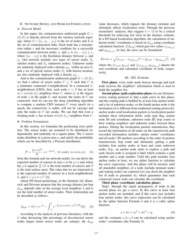
Step2: because the coordinate of unknown node has twoparameters in two dimension: x and y, two formulae arerequired to calculate the coordinate of unknown node. Weapply the hop-count information to getting another formula.We can use Fig. 1 to explain how to get the second formula.Let A and B be the fixed anchor nodes and P be an unknownnode (A and B are predecessor anchor node and successoranchor node for unknown node P respectively. A and B arenearest anchor nodes from node P and they are on the samecurve). The locus of a node P is a circle (this circle is calledlocus circle) where the distance from node A and B is in aconstant ratio: AP : PB = m : n (m and n are the countinghops from node A to P and B to P , respectively and m 6= n.If m = n, the locus of a node P is the perpendicular bisectorof the segment AB) and the diameter length of this locuscircle is IE where I is the internal division point and E isthe external division point of AB.

B , B( x y )I, I( x y )A , A( x y )

O O( x , y )

E E( x , y )

Figure 1. The circle O is P ’s locus circle, and the coordinate is (xo, yo)

Using following method can get another coordinate cal-culation formula:

We can use Formula 6 to get the coordinates of node Iand node E:

xI = mxB+nxAm+n , yI = myB+nyA

m+n ,

xE = mxB−nxAm−n , yE = myB−nyA

m−n ,(6)

and then we can calculate the coordinate of point O usingFormulae [7-8].

First, we calculate the Euclidean distance from I to Eand the radius of circle O: r:

d =√

(xE − xI)2 + (yE − yI)2, and, r =d

2. (7)

Then, calculation the intersection of two circles uses theFormula 8 (this intersection is the O’s coordinate (xo, yo)).

(x− xI)2 + (y − yI)2 = r2,(x− xE)2 + (y − yE)2 = r2.

(8)

Finally, the expression of locus circle is Formula 9:

(xP − xo)2 + (yP − yo)2 = r2, (9)

and the curve expression is Formula 10:

yP = a+ bxP + cx2P + dx3P . (10)

We can use Formulae 9 and 10 to calculate the coordinateof P , but we get two values when m 6= n. In order to findan unique coordinate of P , another anchor node C needsto be chosen (C is also on the same curve), and get otherlocus circles of P using (A and C) and (B and C) asfixed points; the intersection of these circles and curve isthe unique coordinate of P . In case m = n, the P ’s locus isa perpendicular bisector of the segment AB, so we can onlyuse perpendicular bisector expression and curve Formula 10to get an unique coordinate of P .

Fourth phase (optimal phase): in the second path ex-ploration phase, the path circle problem will be caused.We need to eliminate path circle in order to calculate thenodes’ coordinates with the curve expression and improvethe positioning accuracy.

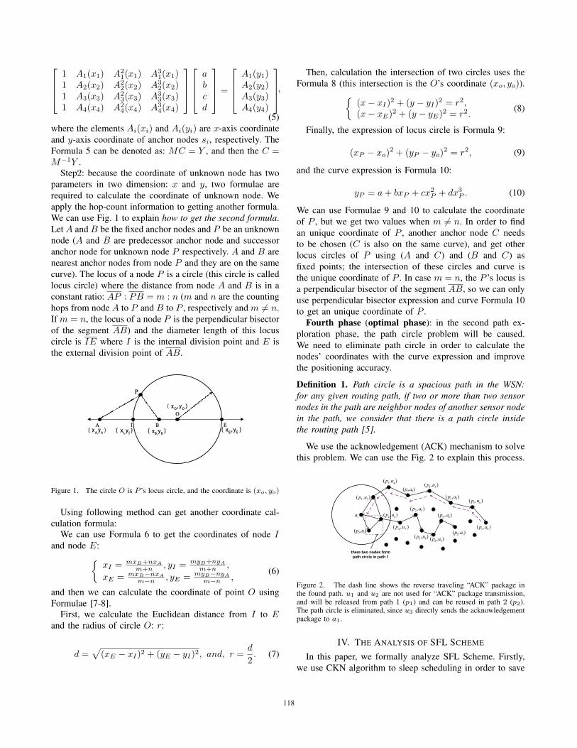
Definition 1. Path circle is a spacious path in the WSN:for any given routing path, if two or more than two sensornodes in the path are neighbor nodes of another sensor nodein the path, we consider that there is a path circle insidethe routing path [5].

We use the acknowledgement (ACK) mechanism to solvethis problem. We can use the Fig. 2 to explain this process.

1 4( , )p a

there two nodes formpath circle in path 1

1 3( , )p u

1a 2 2( , )p u

2 1( , )p u 2 7( , )p u

2 5( , )p a2 6( , )p a

2 7( , )p a

1 2( , )p a1 4( , )p u

1 3( , )p a

1 5( , )p u

1 6( , )p u

2 8( , )p u2 9( , )p u

Figure 2. The dash line shows the reverse traveling “ACK” package inthe found path. u1 and u2 are not used for “ACK” package transmission,and will be released from path 1 (p1) and can be reused in path 2 (p2).The path circle is eliminated, since u3 directly sends the acknowledgementpackage to a1.

IV. THE ANALYSIS OF SFL SCHEME

In this paper, we formally analyze SFL Scheme. Firstly,we use CKN algorithm to sleep scheduling in order to save

118

energy. However, in order to keep a good positioning preci-sion for DV-based localization method, a certain number ofconnected neighbors of a node (CMANS) needs to be guar-anteed. Our SFL method inherits the strong points of DV-based localization method: cost-effective and high-precisionand in the TVC network (node’s sleep scheduling inducesthis phenomenon) our scheme can guarantee accuracy withsmall waking neighbors. That is to say, SFL scheme savesmore energy and at the same time, ensures the positioningaccuracy. Why SFL can ensure a certain accuracy? (i) SFLdoes not need the shortest path (in the previous studies,getting shortest path in a DV-based localization algorithmis NP-Complete, and only can get a near optimal shortestpath, so the localization accuracy is not high) to calculatethe coordinate of unknown node; (ii) our algorithm avoidsthe path circle, which decreases the accumulated error (e.g.,in the DV-based localization method, the path circle makesthe distance between an unknown node and an anchor nodebecomes longer than circle-free path); (iii) SFL scheme doesnot use the “dhop” information to calculate the coordinates,so our method avoids the distance calculation error.

The next theorems show the expected number of rounds inorder to get a smooth curve expression in the second phaseof SFL scheme.

Theorem 1. Consider the routing method of SFL scheme ateach round, which moves one hop to the forward directionwith probability p and moves one hop back direction withprobability q (routing along a forward direction produces asmooth curve), where p > q. Then the expected number ofrounds reaching the end anchor node in a curve is n/(p−q)(at least four anchor nodes in a curve are needed in SFLscheme), where n is the minimum distance in hops to theend anchor node (in SFL method the end node of curve isanchor node and minimum number of hops means that thecurve is smooth without back hop).

Proof: Consider a random walk starting from a node atthe number of hops n from the end node of curve. Let E(n)be the expected number of rounds to get a smooth curvefrom the number of hops n ≥ 0. Because of E(0) = 0, then > 0, and if the node belongs to back direction, we onlyrelease it from current curve,

E(n) = 1+p∗E(n−1)+q∗E(n+1)+(1−p−q)E(n), (11)

this equation’s solution is E(n) = np−q .

The theorem 1 is extended from [6], and it shows: howmany rounds are needed until founding the smooth curve.

Theorem 2. Consider the routing method of SFL scheme ateach round, with probability q bears to back direction, andwith probability p moves to forward node, and in order toget the upper bound of expected number of rounds, we citea result from previous study: with probability pt−1 moves atleast r t−1t (r is radio radius) closer to the fourth anchor

node (in our method we use at least four anchor nodes,because of calculation the upper bound, we can use fouranchor nodes to get optimal upper bound), where t ≥ 2 andt−1∑i=1

i ∗ pi > q ∗ t. Then the expected number of rounds is:

nr ∗

1

( 1t

t−1∑i=1

i ∗ pi)− q, where the r is the distance of one hop

between a pair of nodes.

Proof: Consider a random walk starting from a node.Let E(n) be the expected number of rounds in order to geta smooth curve within n hops and r radio radius:

E(n) ≤ 1

r+

t−1∑i=0

piE(n− i

t) + qE(n+ 1). (12)

Then, we calculate the value of E(n) to get a upper boundabout the expected number of rounds.

First, according to theorem 1’s proof, the value of E(n)has a form: n

x . Second, we use the Equation 12 to get a

expression: n ≤ xr +

t−1∑i=0

pi(n −i

t) + q(n + 1), and further

get (1−t−1∑i=0

pi− q)n ≤x

r−t−1∑i=0

pi(i

t) + q. Because p and q

are probability and p+ q = 1 (in this theorem, p =t−1∑i=0

pi),

1 −t−1∑i=0

pi − q = 0. Finally, we can get x’s bound x ≥

r(

t−1∑i=0

pii

t−q) and according to the formula: E(n) = n

x , we

can obtain E(n) ≤ n

r(

t−1∑i=0

pii

t− q)

.

The theorem 2 is also extended from [6], and it shows: theupper bound rounds are needed until founding the smoothcurve.

V. SIMULATION

A. Simulation Setup

Our WSN is deployed with 500 sensor nodes and thenetwork size is 500(length)×500(width)m2. Moreover, weuse 100 different seeds to generate 100 different network de-ployments (different deployment denotes different topologystructure and the topology of CKN algorithm is variationalbetween different epochs because of sleep scheduling).

B. Simulation Results and Analysis

In our simulation experiments, we compare three local-ization algorithms (a classical localization algorithm: DV-Hop [7], a new positioning algorithm: HCRL [8] and our

119

localization method: SFL) from two different performancespositioning accuracy and energy consumption under dif-ferent anchor node densities: from 20% to 50%. And we

use error =n∑i=1

∆rinR

(∆ri =√

∆x2i + ∆y2i and R is the

communication radius of sensor node) to calculate error asour estimated error.

2600000

Run times(x axis) and Remaining Energy(y axis)

1 2 3 4 5 6 7 8 9 10

SFL 2498599 2497239 2495879 2494521 2493145 2491780 2490400 2489032 2487724 2486368

DVHOP 2315644 2298521 2281398 2264275 2247152 2230029 2212906 2195783 2178659 2161536

HCRL 2315931 2299096 2282260 2265424 2248588 2231752 2214916 2198080 2181244 2164408

1900000

2000000

2100000

2200000

2300000

2400000

2500000

2600000

Rem

ain

ing En

ergy

Run times(x axis) and Remaining Energy(y axis)

(a) Comparison of the energy con-sumption of the three original po-sitioning algorithms with anchornode density 20%

3000000Run times(x axis) and Remaining Energy(y axis)

1 2 3 4 5 6 7 8 9 10

SFL 2499211 2498395 2497570 2496771 2495978 2495166 2494367 2493562 2492792 2491940

DVHOP 2208016 2165777 2123537 2081297 2039057 1996817 1954578 1912338 1870098 1827858

HCRL 2208375 2166494 2124613 2082732 2040851 1998971 1957090 1915209 1873328 1831447

0

500000

1000000

1500000

2000000

2500000

3000000

Rem

ain

ing Ene

rgy

Run times(x axis) and Remaining Energy(y axis)

(b) Comparison of the energy con-sumption of the three original po-sitioning algorithms with anchornode density 30%

3000000Run times(x axis) and Remaining Energy(y axis)

1 2 3 4 5 6 7 8 9 10

SFL 2499502 2498973 2498464 2497942 2497436 2496924 2496400 2495872 2495364 2494831

DVHOP 2113488 1985463 1857437 1729412 1601387 1473362 1345338 1217355 1089466 961723

HCRL 2113926 1986340 1858754 1731167 1603581 1475995 1348409 1220865 1093409 966100

0

500000

1000000

1500000

2000000

2500000

3000000

Rem

ain

ing Ene

rgy

Run times(x axis) and Remaining Energy(y axis)

(c) Comparison of the energy con-sumption of the three original po-sitioning algorithms with anchornode density 40%

Run times(x axis) and Remaining Energy(y axis)

1 2 3 4 5 6 7 8 9 10

SFL 2499659249932324989922498647249830424979642497633249728424969362496600

DVHOP 20217071796525157134313461621120988 895940 671292 447238 223788 838.594

HCRL 20221551797421157268713479531123227 898626 674417 450801 227785 5270.54

0

500000

1000000

1500000

2000000

2500000

3000000

Rem

ain

ing En

erg

y

Run times(x axis) and Remaining Energy(y axis)

(d) Comparison of the energy con-sumption of the three original po-sitioning algorithms with anchornode density 50%

Figure 3. Comparison of the energy consumption of the three originalpositioning algorithms

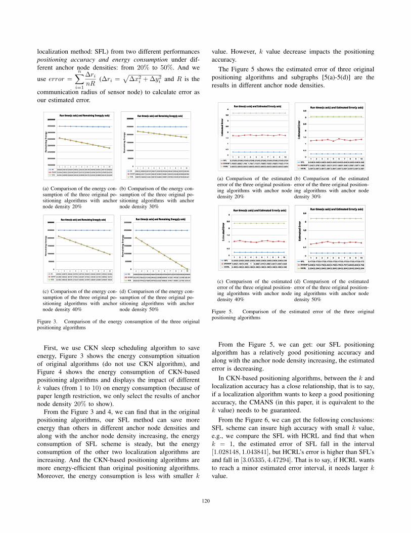
First, we use CKN sleep scheduling algorithm to saveenergy, Figure 3 shows the energy consumption situationof original algorithms (do not use CKN algorithm), andFigure 4 shows the energy consumption of CKN-basedpositioning algorithms and displays the impact of differentk values (from 1 to 10) on energy consumption (because ofpaper length restriction, we only select the results of anchornode density 20% to show).

From the Figure 3 and 4, we can find that in the originalpositioning algorithms, our SFL method can save moreenergy than others in different anchor node densities andalong with the anchor node density increasing, the energyconsumption of SFL scheme is steady, but the energyconsumption of the other two localization algorithms areincreasing. And the CKN-based positioning algorithms aremore energy-efficient than original positioning algorithms.Moreover, the energy consumption is less with smaller k

value. However, k value decrease impacts the positioningaccuracy.

The Figure 5 shows the estimated error of three originalpositioning algorithms and subgraphs [5(a)-5(d)] are theresults in different anchor node densities.

2

2.5

3

3.5

4

stim

ated

Err

or

Run times(x axis) and Estimated Error(y axis)

1 2 3 4 5 6 7 8 9 10

SFL 0.27240.27240.27240.27240.27240.27240.27240.27240.27240.2724

DVHOP 1.70951.6892 1.748 1.768 1.71271.75891.73951.70291.77621.7174

HCRL 3.68533.68533.68533.68533.68533.68533.68533.68533.68533.6853

0

0.5

1

1.5

2

2.5

3

3.5

4

Estim

ated

Err

or

Run times(x axis) and Estimated Error(y axis)

(a) Comparison of the estimatederror of the three original position-ing algorithms with anchor nodedensity 20%

1 5

2

2.5

3

3.5

stim

ated

Err

or

Run times(x axis) and Estimated Error(y axis)

1 2 3 4 5 6 7 8 9 10

SFL 0.246 0.246 0.246 0.246 0.246 0.246 0.246 0.246 0.246 0.246

DVHOP 1.243 1.278 1.282 1.333 1.213 1.388 1.306 1.259 1.307 1.348

HCRL 3.081 3.081 3.081 3.081 3.081 3.081 3.081 3.081 3.081 3.081

0

0.5

1

1.5

2

2.5

3

3.5

Estim

ated

Err

or

Run times(x axis) and Estimated Error(y axis)

(b) Comparison of the estimatederror of the three original position-ing algorithms with anchor nodedensity 30%

2

2.5

3

ated

Err

or

Run times(x axis) and Estimated Error(y axis)

1 2 3 4 5 6 7 8 9 10

SFL 0.2390.2390.2390.2390.2390.2390.2390.2390.2390.239

DVHOP 1.0421.1041.018 1 0.9681.0721.0961.0211.0541.024

HCRL 2.3862.3862.3862.3862.3862.3862.3862.3862.3862.386

0

0.5

1

1.5

2

2.5

3

Estim

ated

Err

or

Run times(x axis) and Estimated Error(y axis)

(c) Comparison of the estimatederror of the three original position-ing algorithms with anchor nodedensity 40%

1

1.5

2

2.5

Estim

ated

Err

or

Run times(x axis) and Estimated Error(y axis)

1 2 3 4 5 6 7 8 9 10

SFL 0.173 0.173 0.173 0.173 0.173 0.173 0.173 0.173 0.173 0.173

DVHOP 0.698 0.743 0.794 0.843 0.768 0.796 0.767 0.808 0.802 0.768

HCRL 2.204 2.204 2.204 2.204 2.204 2.204 2.204 2.204 2.204 2.204

0

0.5

1

1.5

2

2.5

Estim

ated

Err

or

Run times(x axis) and Estimated Error(y axis)

(d) Comparison of the estimatederror of the three original position-ing algorithms with anchor nodedensity 50%

Figure 5. Comparison of the estimated error of the three originalpositioning algorithms

From the Figure 5, we can get: our SFL positioningalgorithm has a relatively good positioning accuracy andalong with the anchor node density increasing, the estimatederror is decreasing.

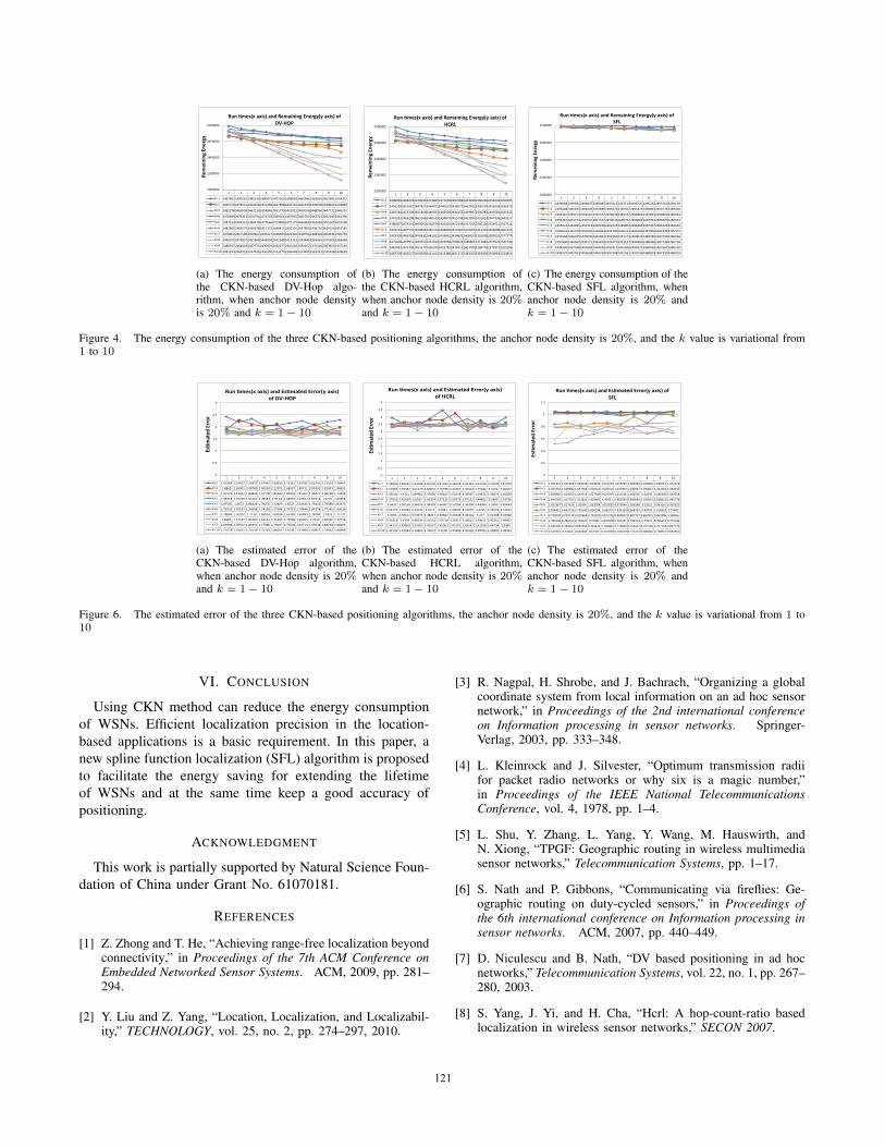
In CKN-based positioning algorithms, between the k andlocalization accuracy has a close relationship, that is to say,if a localization algorithm wants to keep a good positioningaccuracy, the CMANS (in this paper, it is equivalent to thek value) needs to be guaranteed.

From the Figure 6, we can get the following conclusions:SFL scheme can insure high accuracy with small k value,e.g., we compare the SFL with HCRL and find that whenk = 1, the estimated error of SFL fall in the interval[1.028148, 1.043841], but HCRL’s error is higher than SFL’sand fall in [3.05335, 4.47294]. That is to say, if HCRL wantsto reach a minor estimated error interval, it needs larger kvalue.

120

1 2 3 4 5 6 7 8 9 10

K=1 2497462249028124855762480075247226524680592465994246282424613812459312

K=2 2466750245855124543582451438244788824455162441299243960824386452436889

K=3 2465978246365824621202454846245177024510212450039244896024477222445291

K=4 2478989247621324747542471729246916124679552465763246372424621852461336

K=5 2487233248533124804782477666247388624711752466608246160424551652452100

K=6 2482885246927524566782451172244841124421012437965243411024291562416191

K=7 2478863246758924594622445427243869324263202418794240830224046342396793

K=8 2490072247383724578402446939243114824153132399445238346523753062366498

K=9 2480937246460324477752430929242227724054262390367237931823636532347144

K=10 2481294246421924471462430250241327423963482379405236242223454582328639

2300000

2350000

2400000

2450000

2500000

Rem

aini

ng E

nerg

y

Run times(x axis) and Remaining Energy(y axis) of DV-HOP

(a) The energy consumption ofthe CKN-based DV-Hop algo-rithm, when anchor node densityis 20% and k = 1− 10

1 2 3 4 5 6 7 8 9 10

K=1 2498056248647824780042474847247166924670682463046246026424582462456095

K=2 2456209245166724478272444911244020724366752432302243027024283282426319

K=3 2460344245522824514602449023244603924441532439907243628324335812431610

K=4 2470181246629824631662460539245807924557082453995245161424479362443277

K=5 2480607247414524690002463578245630124523492447015244022024344112427111

K=6 2479159246755524599632445724243980924276672419025241332024060892401235

K=7 2473700246676824583322441262243386124248722408209239109823850352377779

K=8 2472658245995124495532431014241696823986242380861237308523559222345748

K=9 2483963247378924552772436979242578324149132403709238477823739732355056

K=10 2487700246922724500002431415241238824011752382023236300023438832324856

2300000

2350000

2400000

2450000

2500000

Rem

aini

ng E

nerg

y

Run times(x axis) and Remaining Energy(y axis) of HCRL

(b) The energy consumption ofthe CKN-based HCRL algorithm,when anchor node density is 20%and k = 1− 10

1 2 3 4 5 6 7 8 9 10

K=1 2499688249909124986472498085249761324971192496727249623224957602495170

K=2 2496408249549324946492493899249307624925022491825249089324901732489426

K=3 2494287249337424925072491537249063624897872488882248789324868002486033

K=4 2494287249337424925072491537249063624897872488882248789324868002486033

K=5 2495622249448524933182492236249102524898032488485248734724862062484920

K=6 2496633249544024942842493064249179024905342489286248796824867392485507

K=7 2497668249639524950902493863249256024912732490025248878024875962486368

K=8 2497890249658724951712493879249247724911472489806248846624871082485758

K=9 2498390249703824956832494296249291724916062490277248892824876072486218

K=10 2498377249703324956682494330249290824915612490196248882024873902486019

2300000

2350000

2400000

2450000

2500000

Rem

aini

ng E

nerg

y

Run times(x axis) and Remaining Energy(y axis) of SFL

(c) The energy consumption of theCKN-based SFL algorithm, whenanchor node density is 20% andk = 1− 10

Figure 4. The energy consumption of the three CKN-based positioning algorithms, the anchor node density is 20%, and the k value is variational from1 to 10

1 2 3 4 5 6 7 8 9 10

K=1 2.41969 2.19027 2.33975 2.07462 2.08633 2.15161 2.25785 2.06141 2.22303 2.28402

K=2 1.8869 2.26901 2.08785 2.00539 2.12371 1.68927 1.89711 2.09392 1.81943 1.98691

K=3 1.99779 1.91421 1.80895 1.91708 1.85943 1.85959 1.81951 1.90471 2.08728 1.73038

K=4 1.88213 1.79339 1.66161 1.78543 1.9134 1.88967 1.92652 1.81914 1.6701 1.80468

K=5 1.87595 1.6673 1.88323 1.79276 1.72805 1.8223 2.02631 1.79222 1.79388 1.83375

K=6 1.75516 1.70157 1.78588 1.74238 1.77096 1.79717 1.74446 1.87074 1.77745 1.69618

K=7 1.78843 1.76972 1.7714 1.83914 1.69204 1.66182 1.66099 1.78783 1.7474 1.71777

K=8 1.6605 1.77747 1.81687 1.63131 1.75204 1.75589 1.69465 1.7617 1.82392 1.72518

K=9 1.69598 1.70512 1.66352 1.77986 1.78197 1.70376 1.64714 1.69038 1.68238 1.80205

K=10 1.77078 1.75011 1.70133 1.75318 1.86051 1.6746 1.57904 1.69817 1.79992 1.66989

0

0.5

1

1.5

2

2.5

3

Estim

ated

Err

or

Run times(x axis) and Estimated Error(y axis) of DV-HOP

(a) The estimated error of theCKN-based DV-Hop algorithm,when anchor node density is 20%and k = 1− 10

1 2 3 4 5 6 7 8 9 10

K=1 3.92946 3.49622 3.32046 3.85192 4.47294 3.56132 3.05335 3.61146 3.53939 3.97359

K=2 3.50387 3.63582 3.61279 3.80852 3.76598 4.24767 3.36424 3.75646 3.3154 3.60472

K=3 3.33542 3.4151 3.09962 3.47801 3.59105 3.53545 3.59397 3.29871 3.48474 3.40004

K=4 3.27016 3.43534 3.6583 3.41334 3.37122 3.59579 3.87131 3.44682 3.2409 3.53756

K=5 3.4432 3.38158 3.36056 3.48393 3.44002 3.53184 3.36994 3.44084 3.5589 3.49643

K=6 3.34173 3.55069 3.44019 3.3217 3.5081 3.49097 3.24975 3.3795 3.53529 3.52815

K=7 3.4091 3.48117 3.54976 3.38227 3.38822 3.40346 3.38301 3.477 3.42308 3.34968

K=8 3.40112 3.4354 3.48934 3.35531 3.39718 3.39357 3.42012 3.38411 3.43215 3.49407

K=9 3.44155 3.43854 3.32693 3.40327 3.45063 3.43191 3.43242 3.41398 3.44734 3.3985

K=10 3.43136 3.42084 3.39805 3.40072 3.4108 3.44989 3.40429 3.39784 3.39805 3.38493

0

0.5

1

1.5

2

2.5

3

3.5

4

4.5

5

Estim

ated

Err

or

Run times(x axis) and Estimated Error(y axis) of HCRL

(b) The estimated error of theCKN-based HCRL algorithm,when anchor node density is 20%and k = 1− 10

1 2 3 4 5 6 7 8 9 10

K=1 1.041841 1.041265 1.028148 1.043841 1.041703 1.043765 1.028284 1.040802 1.030951 1.042326

K=2 1.027418 1.039806 1.037384 1.030616 1.020314 1.037904 1.030937 1.040027 1.022218 1.042435

K=3 1.029866 1.024055 1.042354 1.027929 1.023295 1.011516 1.042605 1.02345 1.036369 1.044058

K=4 1.044766 1.017707 1.021821 1.039465 1.00421 0.982935 0.996869 1.033015 1.028623 1.045778

K=5 1.023367 1.017326 1.01504 1.013204 1.052825 0.973844 1.026248 1.02011 0.993161 0.992522

K=6 0.838411 0.862716 0.795142 0.850294 0.86274 0.839328 0.966793 0.84793 1.018543 0.97405

K=7 0.790997 0.794174 0.818664 0.781833 0.831728 0.809002 0.807317 0.860915 0.862486 0.88066

K=8 0.781994 0.780231 0.759247 0.72081 0.807506 0.762331 0.799724 0.79722 0.765657 0.723106

K=9 0.581005 0.784301 0.845265 0.742431 0.785887 0.773804 0.703451 0.703749 0.707704 0.807779

K=10 0.521931 0.53164 0.643365 0.67325 0.731939 0.701619 0.772272 0.683845 0.730917 0.691652

0

0.2

0.4

0.6

0.8

1

1.2

Esti

mat

ed E

rror

Run times(x axis) and Estimated Error(y axis) of SFL

(c) The estimated error of theCKN-based SFL algorithm, whenanchor node density is 20% andk = 1− 10

Figure 6. The estimated error of the three CKN-based positioning algorithms, the anchor node density is 20%, and the k value is variational from 1 to10

VI. CONCLUSION

Using CKN method can reduce the energy consumptionof WSNs. Efficient localization precision in the location-based applications is a basic requirement. In this paper, anew spline function localization (SFL) algorithm is proposedto facilitate the energy saving for extending the lifetimeof WSNs and at the same time keep a good accuracy ofpositioning.

ACKNOWLEDGMENT

This work is partially supported by Natural Science Foun-dation of China under Grant No. 61070181.

REFERENCES

[1] Z. Zhong and T. He, “Achieving range-free localization beyondconnectivity,” in Proceedings of the 7th ACM Conference onEmbedded Networked Sensor Systems. ACM, 2009, pp. 281–294.

[2] Y. Liu and Z. Yang, “Location, Localization, and Localizabil-ity,” TECHNOLOGY, vol. 25, no. 2, pp. 274–297, 2010.

[3] R. Nagpal, H. Shrobe, and J. Bachrach, “Organizing a globalcoordinate system from local information on an ad hoc sensornetwork,” in Proceedings of the 2nd international conferenceon Information processing in sensor networks. Springer-Verlag, 2003, pp. 333–348.

[4] L. Kleinrock and J. Silvester, “Optimum transmission radiifor packet radio networks or why six is a magic number,”in Proceedings of the IEEE National TelecommunicationsConference, vol. 4, 1978, pp. 1–4.

[5] L. Shu, Y. Zhang, L. Yang, Y. Wang, M. Hauswirth, andN. Xiong, “TPGF: Geographic routing in wireless multimediasensor networks,” Telecommunication Systems, pp. 1–17.

[6] S. Nath and P. Gibbons, “Communicating via fireflies: Ge-ographic routing on duty-cycled sensors,” in Proceedings ofthe 6th international conference on Information processing insensor networks. ACM, 2007, pp. 440–449.

[7] D. Niculescu and B. Nath, “DV based positioning in ad hocnetworks,” Telecommunication Systems, vol. 22, no. 1, pp. 267–280, 2003.

[8] S. Yang, J. Yi, and H. Cha, “Hcrl: A hop-count-ratio basedlocalization in wireless sensor networks,” SECON 2007.

121