1

Advances in Variational InferenceCheng Zhang Judith Butepage Hedvig Kjellstrom Stephan Mandt

Abstract—Many modern unsupervised or semi-supervised machine learning algorithms rely on Bayesianprobabilistic models. These models are usually intractable and thus require approximate inference. Variationalinference (VI) lets us approximate a high-dimensional Bayesian posterior with a simpler variational distribution bysolving an optimization problem. This approach has been successfully used in various models and large-scaleapplications. In this review, we give an overview of recent trends in variational inference. We first introducestandard mean field variational inference, then review recent advances focusing on the following aspects: (a)scalable VI, which includes stochastic approximations, (b) generic VI, which extends the applicability of VI to alarge class of otherwise intractable models, such as non-conjugate models, (c) accurate VI, which includesvariational models beyond the mean field approximation or with atypical divergences, and (d) amortized VI,which implements the inference over local latent variables with inference networks. Finally, we provide asummary of promising future research directions.

Index Terms—Variational Inference, Approximate Bayesian Inference, Reparameterization Gradients, StructuredVariational Approximations, Scalable Inference, Inference Networks.

F

1 INTRODUCTION

Bayesian inference has become a crucial componentof machine learning. It allows us to systematicallyreason about parameter uncertainty. The central objectof interest in Bayesian inference is the posterior distri-bution of model parameters given observations. Mostmodern applications require complex models, and thecorresponding posterior is beyond reach. Practitioners,therefore, resort to approximations. This review focuseson variational inference (VI): a collection of approxi-mation tools that make Bayesian inference computa-tionally efficient and scalable to large data sets.

Many Bayesian machine learning methods relyon probabilistic latent variable models. These includeGaussian Mixture Models (GMM), Hidden MarkovModels (HMM), Latent Dirichlet Allocation (LDA),Stochastic Block Models, and Bayesian deep learningarchitectures. Exact inference is typically intractablein these models; consequently approximate inferencemethods are needed. In VI, one approximates the modelposterior by a simpler distribution. To this end, one

• Cheng Zhang and Stephan Mandt are with Disney Research,Pittsburgh.E-mail: {cheng.zhang, stephan.mandt}@disneyresearch.com

• Judith Butepage is with KTH Royal Institute of Technology.Her contribution in this work is mainly done during herinternship in Disney Research, Pittsburgh.E-mail: butepage@kth.se

• Hedvig Kjellstrom is with KTH Royal Institute of Technology.E-mail: hedvig@kth.se

minimizes the Kullback-Leibler divergence betweenthe posterior and the approximating distribution. Thisapproach circumvents computing intractable normal-ization constants. It only requires knowledge of thejoint distribution of the observations and the latentvariables. This methodology along with its recent re-finements will be reviewed in this paper.

Within the field of approximate Bayesian inference,VI falls into the class of optimization-based approaches[13], [54]. This class also contains methods such asloopy belief propagation [116] and expectation prop-agation (EP) [113]. On the contrary, Markov ChainMonte Carlo (MCMC) approaches, rely on sampling[19], [53], [134]. Monte Carlo methods are oftenasymptotically unbiased, but can be slow to converge.Optimization-based methods, on the other hand, areoften faster but may suffer from oversimplified pos-terior approximations [13], [181]. In recent years, therehas been considerable progress in both fields [7],[14], and in particular on bridging the gap betweenthese methods [1], [83], [101], [135], [150]. In fact,recent progress in scalable VI partly relies on fus-ing optimization-based and sampling-based methods.While this review focuses on VI, readers interested inEP and MCMC are referred to, e.g., [155] and [7].

The origins of VI date back to the 1980s. Mean fieldmethods, for instance, have their origins in statisticalphysics, where they played a prominent role in thestatistical mechanics of spin glasses, see [107] and[130]. Early applications of variational methods also

arX

iv:1

711.

0559

7v1

[cs

.LG

] 1

5 N

ov 2

017

2

include the study of neural networks, see [127] and[132]. The latter work inspired the computer sciencecommunity of the 1990s to adopt variational methodsin the context of probabilistic graphical models [65],[153], see also [71], [126] for early introductions onthis topic.

In recent years, several factors have driven a re-newed interest in variational methods. The modernversions of VI differ significantly from earlier formula-tions. Firstly, the availability of large datasets triggeredthe interest in scalable approaches, e.g., based onstochastic gradient descent [17], [59]. Secondly, classi-cal VI is limited to conditionally conjugate exponentialfamily models, a restricted class of models describedin [59], [181]. In contrast, black box VI algorithms[66], [71], [135] and probabilistic programs facilitategeneric VI, making it applicable to a range of compli-cated models. Thirdly, this generalization has spurredresearch on more accurate variational approximations,such as alternative divergence measures [94], [114],[194] and structured variational families [137]. Finally,amortized inference employs complex functions suchas neural networks to predict variational distributionsconditioned on data points, rendering VI an importantcomponent of modern Bayesian deep learning architec-tures such as variational autoencoders. In this work, wediscuss important papers concerned with each of thesefour aspects.

While several excellent reviews of VI exist, webelieve that our focus on recent developments in scal-able, generic, accurate and amortized VI goes beyondthose efforts. Both [71] and [126] date back to theearly 2000s and do not cover the developments ofrecent years. Similarly, [181] is an excellent resource,especially regarding structured approximations and theinformation geometrical aspects of VI. However, itwas published prior to the widespread use of stochas-tic methods in VI. Among recent introductions, [14]contains many examples, empirical comparisons, andexplicit model calculations but focuses less on blackbox and amortized inference; [7] focuses mainly onscalable MCMC. Our review concentrates on the ad-vances of the last 10 years prior to the publication ofthis paper. Complementing previous reviews, we skipexample calculations to focus on a more exhaustivesurvey of the recent literature.

Here, we present developments in VI in a self-contained manner. We begin by covering the ba-sics of VI in Section 2. In the following sections,we concentrate on recent advances. We identify fourmain research directions: scalable VI (Section 3), non-conjugate VI (Section 4), non-standard VI (Section 5),and amortized VI (Section 6). We finalize the reviewwith a discussion (Section 7) and concluding remarks(Section 8).

2 VARIATIONAL INFERENCE

We begin this review with a brief tutorial on variationalinference, presenting the mathematical foundations ofthis procedure and explaining the basic mean-fieldapproximation.

Notation: The generative process is specified byobservations xxx, as well as latent variables zzz and ajoint distribution p(xxx,zzz). We use bold font to explic-itly indicate sets of variables, i.e. zzz = {z1,z2, · · · ,zN},where N is the total number of latent variables andxxx = {x1,x2, · · · ,xM}, where M is the total number ofobservations in the dataset. The variational distributionq(zzz;λλλ ) is defined over the latent variables zzz and hasvariational parameters λλλ = {λ1,λ2, · · ·λN}.

2.1 Inference as OptimizationThe central object of interest in Bayesian statisticsis the posterior distribution of latent variables givenobservations:

p(zzz|xxx) = p(xxx,zzz)∫p(xxx,zzz)dzzz

. (1)

For most models, computing the normalization term isimpossible.

In order to approximate the posterior distributionp(zzz|xxx), VI introduces a simpler distribution q(zzz;λλλ ), pa-rameterized by variational parameters λλλ , and a distancemeasure between the the proxy distribution and the trueposterior is considered. We then minimize this distancewith respect to the parameters λλλ . Finally, the optimizedvariational distribution is taken as a proxy for theposterior. In this way, VI turns Bayesian inference intoan optimization problem.

Distance measures between two distributions p(y)and q(y) are also called divergences. As we show be-low, the divergence between the variational distributionand the posterior cannot be minimized directly in VI,because this involves knowledge of the posterior nor-malization constant. Instead, a related quantity can bemaximized, namely a lower bound on the log marginalprobability p(xxx) (this will be explained below).

While various divergence measures exist [4], [6],[114], [161], the most commonly used divergence is theKullback-Leibler (KL) divergence [13], [87], which isalso referred to as relative entropy or information gain:

DKL(q(y)||p(y)) =−∫

q(y) logp(y)q(y)

dy. (2)

As seen in Eq. 2, the KL divergence is asymmet-ric; DKL(q(y)||p(y)) 6= DKL(p(y)||q(y)). Depending onthe ordering, we obtain two different approximateinference methods. As we show below, VI employsDKL(q(zzz)||p(zzz|xxx)) = −Eq(zzz)

[log p(zzz|xxx)

q(zzz)

]. On the other

hand, expectation propagation (EP) [113] optimizes

3

DKL(p(zzz|xxx)||q(zzz)) for local moment matching, whichis not reviewed in this paper1. In Section 5 we discussalternative divergence measures that can improve theperformance of VI.

2.2 Variational Objective

VI aims at determining a variational distribution q(zzz)that is as close as possible to the posterior p(zzz|xxx),measured in terms of the KL divergence. As for alldivergences, DKL(q||p) is only zero if q = p. Thus, inan ideal case, the variational distribution takes the formq(zzz) = p(zzz|xxx). In practice, this is rarely possible; thevariational distribution is usually under-parameterizedand thus not sufficiently flexible to capture the fullcomplexity of the true posterior.

As discussed below, minimizing the KL divergenceis equivalent to maximizing the evidence lower bound(ELBO) L . The ELBO is a lower bound on the logmarginal probability, log p(xxx). Since the ELBO is aconservative estimate of this marginal, which can beused for model selection, the ELBO is sometimes takenas an estimate of how well the model fits the data.

The ELBO L can be derived from log p(xxx) usingJensen’s inequality as follows:

log p(xxx) = log∫

p(xxx,zzz)dzzz = log∫ p(xxx,zzz)q(zzz;λλλ )

q(zzz;λλλ )dzzz

= logEq(zzz;λλλ )

[p(xxx,zzz)q(zzz;λλλ )

]≥ Eq(zzz;λλλ )

[log

p(xxx,zzz)q(zzz;λλλ )

]≡L (λλλ ).

(3)It can be shown (see Appendix A.1) that the differencebetween the true log marginal probability of the dataand the ELBO is the KL divergence between thevariational distribution and the posterior distribution:

log p(xxx) = L (λλλ )+DKL(q||p) (4)

Thus, maximizing the ELBO is equivalent to mini-mizing the KL divergence between q and p. In tra-ditional VI, computing the ELBO amounts to analyti-cally solving the expectations over q, where the modelis commonly restricted to the so-called conditionallyconjugate exponential family (see Appendix A.2 and[181]). As part of this article, we will present moremodern approaches where this is no longer the case.For an exemplary derivation of VI updates for a Gaus-sian Mixture Model, see [14].

The KL divergence between q and p tends toforce q to be close to zero wherever p is zero (zeroforcing) [114]. This property leads to automatic sym-metry breaking, however, it results in underestimating

1. We refer the readers to the EP roadmap for more informa-tion about advancement of EP. https://tminka.github.io/papers/ep/roadmap.html

the variance. In detail, when the posterior has severalequivalent modes caused by model symmetry, KLbased VI may focus on a single mode due to its zeroforcing property. For the same reason, since the vari-ational distribution is commonly not flexible enough,the zero forcing property leads to underestimates ofthe variance. In contrast, MCMC or EP may show anundesirable mode averaging behavior, while estimatingthe variance more closely.

It is important to choose q(zzz) to be simple enoughto be tractable, but flexible enough to provide a goodapproximation of the posterior [13]. A common choiceis a fully factorized distribution, a mean field distri-bution, which is introduced in Section 2.3. A meanfield distribution assumes that all latent variables areindependent, which simplifies derivations. However,this independence assumption also leads less accurateresults especially when the true posterior variablesare highly dependent. This is e.g. the case in timeseries or complex hierarchical models. Richer familiesof distributions may lead to better approximations,but may complicate the mathematics and computation.This motivates extensions such as structured VI whichis reviewed in Section 5.

2.3 Mean Field Variational Inference

Mean Field Variational Inference (MFVI) has its ori-gins in the mean field theory of physics [126]. MFVIassumes that the variational distribution factorizes overthe latent variables:

q(zzz;λλλ ) =N

∏i=1

q(zi;λi). (5)

This independence assumption leads to an approximateposterior that is less expressive than when preservingdependencies, but simplifies algorithms and mathe-matical derivations. For notational simplicity, we omitthe variational parameters λλλ for the remainder of thissection. We now review how to maximize the ELBOL , defined in Eq. 3, under a mean field assumption.

A fully factorized variational distribution allowsone to optimize L via simple iterative updates. To seethis, we focus on updating the variational parameter λ jassociated with latent variable z j. Inserting the meanfield distribution into Eq. 3 allows us to express theELBO as follows:

L =∫

q(z j)Eq(zzz¬ j) [log p(z j,xxx|zzz¬ j)]dz j

−∫

q(z j) logq(z j)dz j + c j.(6)

Above, zzz¬ j indicates the set zzz excluding z j. The con-stant c j contains all terms that are constant with respectto z j, such as the entropy term associated with zzz¬ j. Wehave thus separated the full expectation into an innerexpectation over zzz¬ j, and an outer expectation over z j.

4

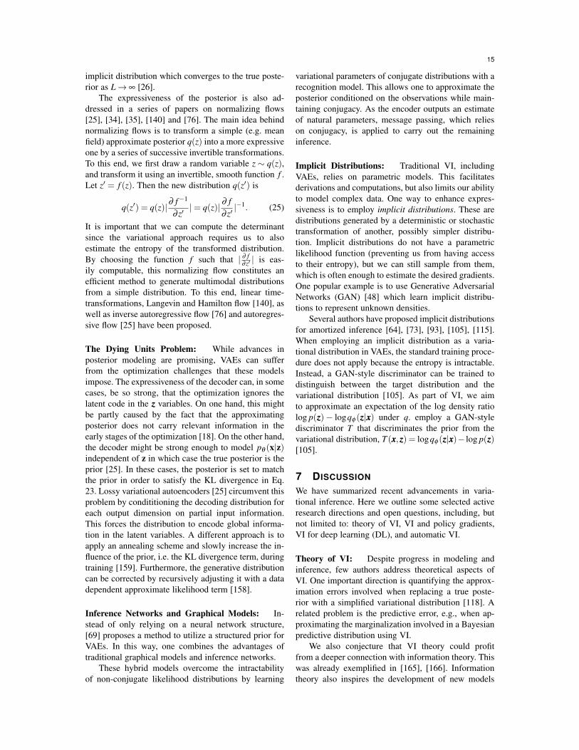
α θ

ξ xM

Fig. 1. A graphical model of the observations xxx that dependon underlying local hidden factors ξξξ and global parametersθ . We use zzz = {θ ,ξξξ} to represent all latent variables. M isthe number of the data points. N is the number of the latentvariables.

Inspecting Eq. 6, it becomes apparent that this for-mula is a negative KL divergence, which is maximizedfor variable j by:

log q∗(z j) = Eq(zzz¬ j) [log p(z j|zzz¬ j,xxx)]+ const. (7)

Exponentiating and normalizing this result yields:

q∗(z j) ∝ exp(Eq(zzz¬ j) [log p(z j|zzz¬ j,xxx)])

∝ exp(Eq(zzz¬ j) [log p(zzz,xxx)])(8)

Using Eq. 8, the variational distribution can now beupdated iteratively for each latent variable until con-vergence. Similar updates also form the basis for thevariational message passing algorithm [190] (See Ap-pendix A.3).

For more details on the mean field approximationand its geometrical interpretation we refer the readerto [181] and [13]. Having covered the basics of VI,we devote the rest of this paper to reviewing advancedtechniques.

3 SCALABLE VARIATIONAL INFERENCE

In this section, we survey scalable VI. Big datasetsraise new challenges for the computational feasibil-ity of Bayesian algorithms, making scalable inferencetechniques essential. We begin by reviewing stochasticvariational inference (SVI) in Section 3.1, which usesstochastic gradient descent to scale VI to large datasets.Section 3.2 discusses practical aspects of SVI, such asadaptive learning rates or variance reduction. Furtherapproaches to improve on the scalability of VI arediscussed in Section 3.3; these include sparse inference,collapsed inference and distributed inference.

Notation: This section follows the general modelstructure of global and local hidden variables, assumedin [59]. Fig. 1 depicts the corresponding graphicalmodel where the latent variable zzz = {θ ,ξξξ} includeslocal (per data point) variables ξξξ and global variableθ . Similarly, the variational parameters are given byλλλ = {γ,φφφ}, where the variational parameter γ corre-sponds to the global latent variable, and φφφ denotes theset of local variational parameters. Furthermore, the

model depends on hyperparameters α . The mini-batchsize is denoted by S.

3.1 Stochastic Variational Inference

VI frames Bayesian inference as an optimization prob-lem. For many models of interest, the variational ob-jective has a special structure, namely, it is the sumover contributions from all M individual data points.Problems of this type can be solved efficiently usingstochastic optimization [17], [143]. Stochastic Varia-tional Inference (SVI) amounts to applying stochasticoptimization to the objective function encountered inVI [57], [59], [63], [185], thereby scaling VI to verylarge datasets. Using stochastic optimization in thecontext of VI was proposed in [59], [63], [152]. Wefollow the conventions of [59] which presents SVIfor models of the conditionally conjugate exponentialfamily class.

The ELBO of the general graphical model shownin Fig. 1 has the following form:

L = Eq[log p(θ |α)− logq(θ |γ)]+ (9)M

∑i=1

Eq[

log p(ξi|θ)+ log p(xi|ξi,θ)− logq(ξi|φi)].

We assume that the variational distribution is givenby q(ξξξ ,θ) = q(θ |γ)∏

Mi=1 q(ξi|φi). For conditionally

conjugate exponential families [181], the expectationsinvolved in Eq. 9 can be computed analytically, yield-ing a closed form objective that can be optimizedwith coordinate updates. In this case, every iteration orgradient step scales with M, and is therefore expensivefor large data.

SVI solves this problem by randomly selectingmini-batches of size S to obtain a stochastic estimateof the ELBO L :

L = Eq[log p(θ |α)− logq(θ |γ)]+ (10)

MS

S

∑s=1

Eq[

log p(ξis |θ)+ log p(xis |ξis ,θ)− logq(ξis |φis)],

where is is the variable index from the mini-batch.This objective is optimized using stochastic gradientascent. The mini-batch size is chosen as S� M withS > 1 in order to reduce the variance of the gradient.The choice of S emerges from a trade-off between thecomputational overhead associated with processing amini-batch, such as performing inference over globalparameters (favoring larger mini-batches which havelower gradient noise and allow larger learning rate),and the cost of iterating over local parameters in themini-batch (favoring small mini-batches). Additionally,this tradeoff is also affected by memory structures inmodern hardware such as GPUs.

As in stochastic optimization, SVI requires the useof a learning rate ρt that decreases over iterations t. The

5

Robbins-Monro conditions ∑∞t=1 ρt = ∞ and ∑

∞t=1 ρ2

t <∞ guarantee that every point in parameter space canbe reached, while the gradient noise decreases quicklyenough to ensure convergence [143]. We deepen thediscussion of these topics in Section 3.2.

An important result of [59] is that the SVI proce-dure automatically produces natural stochastic gradi-ents, and that these natural gradients have a simplerform than regular gradients for models in the condi-tionally conjugate exponential family. Natural gradientsare studied in [5] and were first introduced to VI in[61], [62]. They are pre-multiplied with the inverseFisher information and therefore take the informationgeometry into account. For details, we refer interestedreaders to Appendix A.4 and [59].

Sometimes SVI is referred to as online VI [57],[185]. These methods are equivalent under the assump-tions that the volume of the data M is known. In stream-ing applications, the mini-batches arrive sequentiallyfrom a data source, but the SVI updates look the same.However, when M is unknown, it is unclear how toset the scale parameter M/S in Eq. 10. To this end,[104] introduces the concept of the population posteriorwhich depends on the unknown size of the dataset. Thisconcept allows one to apply online VI with respect tothe expected ELBO over the population.

Stochastic gradient methods have been adaptedto various settings, such gamma processes [82] andvariational autoencoders [79]. In recent years, mostadvancements in VI have been developed relying on aSVI scheme. In the following, we detail how to furtheradapt SVI to accelerate convergence.

3.2 Tricks of the Trade for SVIThe efficiency of stochastic gradient descent (SGD)methods, which are the basis of SVI, depend on thevariance of the gradient estimates. Smaller gradientnoise allows for larger learning rates and leads to fasterconvergence. This section covers tricks of the tradein the context of SVI, such as adaptive learning ratesand variance reduction. Some of these approaches aregenerally applicable in SGD setups.

Adaptive Learning Rate and Mini-batch Size:The speed of convergence is influenced by the choiceof the learning rate and the mini-batch size [9], [40].Due to the law of large numbers, increasing the mini-batch size reduces the stochastic gradient noise [40],allowing larger learning rates. To accelerate the learn-ing procedure, one can either optimally adapt the mini-batch size for a given learning rate, or optimally adjustthe learning rate to a fixed mini-batch size.

We begin by discussing learning rate adaptation.In each iteration, the empirical gradient variance canguide the adaptation of the learning rate. Popular op-timization methods that make use of this idea include

RMSProp [170], AdaGrad [36], AdaDelta [191] andAdam [80]. These methods are not specific to SVI butare frequently used in this context; for more details werefer interested reader to [47]. An adaptive learning ratespecifically designed for SVI was suggested in [138].Recall that γ is the global variational parameter. Thelearning rate for γ results from minimizing the errorbetween the stochastic mini-batch update and the fullbatch update, and is given by:

ρ∗t =

(γ∗t − γt)T (γ∗t − γt)

(γ∗t − γt)T (γ∗t − γt)+ tr(Σ), (11)

where γ∗t indicates the batch update (using all data),γt is the current variational parameter and Σ is thecovariance matrix of the variational parameter in thismini-batch. Eq. 11 indicates that the learning rateshould increase when the trace term, i.e. the mini-batchvariance, is small. Further estimation of ρt is presentedin [138]. Although developed for SVI, this method canbe adapted to other stochastic optimization methodsand resembles the aforementioned adaptive learningrate schemes.

Instead of adapting the learning rate, the mini-batch size can be adapted while keeping the learningrate fixed to achieve similar effects [9], [22], [31]. Forexample [9] optimizes the mini-batch size to decreasethe SGD variance proportionally to the value of theobjective function relative to the optimum. In practice,the estimated gradient noise covariance and the mag-nitude of the gradient are used to estimate the optimalmini-batch size.

Variance Reduction: In addition to controllingthe optimization path through the learning rate andmini-batch size, we can reduce the variance, therebyenabling larger gradient steps. Variance reduction isoften employed in SVI to achieve faster convergence.In the following, we summarize how to accomplish thiswith control variates, non-uniform sampling, and otherapproaches.

Control Variates. A control variate is a stochasticterm that can be added to the stochastic gradient suchthat its expectation remains the same, but its varianceis reduced. It is constructed as a vector that shouldbe highly correlated with the stochastic gradient andeasy to compute. Using control variates for variancereduction is common in Monte Carlo simulation andstochastic optimization [146], [184]. Several authorshave suggested the use of control variates in the contextof SVI [70], [129], [135], [184]. [184] provides two ex-amples of model specific control variate construction,focusing on logistic regression and LDA.

The stochastic variance reduced gradient (SVRG)method [70] amounts to constructing a control variatewhich takes advantage of previous gradients from all

6

data points. It exploits that gradients along the opti-mization path are correlated. The standard stochasticgradient update γt+1 = γt −ρt(∇L (γt)) is replaced by:

γt+1 = γt −ρt(∇L (γt)−∇L (γ)+ µ). (12)

L indicates the estimated objective (here the negativeELBO) based on the current set of mini-batch indices,γ is a snapshot of γ after every m iterations, and µ isthe batch gradient computed over all the data points,µ = ∇L (γ). Since SVRG requires a full pass throughthe dataset every mth iteration, it is not feasible forvery large datasets. Yet, in contrast to traditional SGD,SVRG enables convergence with constant learningrates. We will encounter different types of control vari-ates in the context of black box variational inference(BBVI) (see Section 4.2 for a detailed discussion).

Non-uniform Sampling. Instead of subsamplingdata points with equal probability, non-uniform sam-pling can be used to select mini-batches with a lowergradient variance. Several authors suggested variantsof importance sampling in the context of mini-batchselection [27], [131], [198]. Although effective, thesemethods are not always practical, as the computa-tional complexity of the sampling probability relatesto the dimensionality of model parameters [41]. Al-ternative methods aim at de-correlating similar pointsand sampling diversified mini-batches. These methodsinclude stratified sampling [197], where one samplesdata from pre-defined subgroups based on meta-data orlabels, clustering-based sampling [41], which amountsto clustering the data using k-means and then samplingdata from every cluster with adjusted probabilities, anddiversified mini-batch sampling [196] using determi-nantal point processes (see Appendix A.5) to suppressthe probability of data points with similar features inthe same mini-batch. All of these methods have beenshown to reduce variance and can also be used forlearning on imbalanced data.

Other Methods. A number of alternative methodshave been developed that contribute to variance re-duction for SVI. A popular approach relies on Rao-Blackwellization, which is used in [135]. The Rao-Blackwellization theorem (see Appendix A.6) gen-erally states that a conditional estimation has lowervariance if a valid statistic to be conditioned on exists.Inspired by Rao-Blackwellization, the local expectationgradients method [173], [176] has been proposed. Itexplores the conditional structure of a model to reducethe variance. A related approach has been developed forSVI, which averages expected sufficient statistics overa sliding window of mini-batches to obtain a naturalgradient with smaller mean squared error [100]. Fur-ther variance reduction methods [77], [135], [144] aredesigned for black box variational inference (BBVI).

These methods make use of the reparametrization trickand are discussed together with BBVI in Section 4.They are different in nature because the samplingspace is continuous, while SVI samples from a discretepopulation of data points.

3.3 Collapsed, Sparse, and Distributed VIIn contrast to using stochastic optimization for fasterconvergence, this section presents methods that lever-age the structure of certain models to achieve thesame goal. In particular, we focus on collapsed, sparse,parallel, and distributed inference.

Collapsed Inference: Collapsed variational infer-ence (CVI) relies on the idea of analytically integratingout certain model parameters [56], [75], [88], [90],[162], [167], [175]. Due to the reduced number ofparameters to be estimated, inference is typically faster.One can either marginalize out these latent variablesbefore the ELBO is derived, or eliminate them after-wards [56], [75].

Several authors have proposed CVI for topic mod-els [88], [167] where one can either collapse the topicproportions [167] or the topic assignment [56]. In ad-dition to these model specific derivations, [56] unifiesexisting model-specific CVI approaches and presents ageneral collapsed inference method for models in theconjugate exponential family class.

The computational benefit of CVI depends stronglyon the statistics of the collapsed variables. Additionally,collapsing latent random variables in a model can causeother inference techniques to become tractable. Formodels such as topic models, we can collapse thediscrete variables and only infer the continuous ones,allowing e.g. the application of inference networks(Section 6) [108], [160].

Sparse Inference: Sparse inference aims to exploiteither sparsely distributed parameters for parametricmodels, or datasets which can be summarized by asmall number of representative data points. In theseregimes, low rank approximations enable scalable in-ference [55], [157], [174]. Sparse inference can be ei-ther interpreted as a modeling choice or as an inferencescheme [20].

Sparse inference methods are often encountered inthe Gaussian Process (GPs) literature. The computa-tional cost of learning GPs is O(n3), where n is thenumber of data points. This cost is caused by theinversion of the kernel matrix Knn of size n×n, whichhinders the application of GPs to big data sets. Theidea of sparse inference in GPs [157] is to introducem inducing points. These are auxiliary variables which,when integrated out, yield the original GP. Instead ofbeing marginalized out however, they are treated as

7

latent variables whose distribution is estimated usingVI. Inducing points can be interpreted as pseudo-inputsthat reflect the original data, but yield a more sparserepresentation since m� n. With inducing points, onlya m×m sized matrix needs to be inverted, and conse-quently the computational complexity of this methodis O(nm2). [174] collapses the distribution of inducingpoints, and [55] further extends this work to a stochas-tic version [59] with a computational complexity ofO(m3). Additionally, sparse inducing points make in-ference in Deep Gaussian Processes tractable [30].

Parallel and Distributed Inference: Several com-putational acceleration techniques, such as distributedcomputing, can be applied to VI [43], [120], [123],[192]. Distributed inference schemes are often requiredin large scale scenarios, where data and computationsare distributed across several machines. Independentlatent variable models are trivially parallelizable. How-ever, model specific designs such as reparametrizationsmight be required to enable efficient distributed in-ference [43]. Current computing resources make VIapplicable to web-scale data analysis [192].

4 NON-CONJUGATE INFERENCE

In this section, we review techniques which make VIgeneric. One aspect of this research is to make VImore broadly applicable to a large class of models, inparticular non-conjugate ones. A second aspect is tomake VI more automatic, thus eliminating the need formodel-specific calculations and approximations, whichallows VI to be more accessible in general.

Variational inference was originally limited to con-ditionally conjugate models, for which the ELBO couldbe computed analytically before it was optimized [59],[193]. In this section, we introduce methods that relaxthis requirement and simplify inference. Central to thissection are stochastic gradient estimators of the ELBOthat can be computed for a broader class of models.

We start with the Laplace approximation in Section4.1 and illustrate its limitations. We will then introduceblack box variational inference (BBVI) in Section 4.2which employs the REINFORCE or score functiongradient. Section 4.3 discusses a different form ofBBVI, which uses reparameterization gradients. Otherapproaches for non-conjugate VI are discussed in Sec-tion 4.4.

4.1 Laplace’s Method and Its Limitations

The Laplace (or Gaussian) approximation, estimatesthe posterior by a Gaussian distribution [89]. To thisend, one seeks the maximum of the posterior andcomputes the inverse of its Hessian. These two en-tities are taken as the mean and covariance of the

Gaussian posterior approximation. To make this ap-proach feasible, the log posterior needs to be twice-differentiable. According to the Bernstein von Misestheorem (a.k.a. Bayesian central limit theorem) [23],the posterior approaches a Gaussian asymptoticallyin the limit of large data, and the Laplace approx-imation becomes exact (provided that the model isunder-parameterized). The approach can be applied toapproximate the maximum a posteriori (MAP) meanand covariance, predictive densities, and marginal pos-terior densities [171]. The Laplace method has alsobeen extended to more complex models such as beliefnetworks with continuous variables [8].

This approximation suffers mainly from beingpurely local and depending only on the curvature of theposterior around the optimum; KL minimization typi-cally approximates the posterior shape more accurately.Additionally, the Laplace approximation is limited tothe Gaussian variational family and does not apply todiscrete variables [183]. Computationally, the methodrequires the inversion of a potentially large Hessian,which can be costly in high dimensions. This makesthis approach intractable in setups with a large numberof parameters.

4.2 Black Box Variational Inference

In classical variational inference, the ELBO is firstderived analytically, and then optimized. This proce-dure is usually restricted to models in the conditionallyconjugate exponential family [59]. For many models,including Bayesian deep learning architectures or com-plex hierarchical models, the ELBO often contains in-tractable expectations with no known or simple analyt-ical solution. Even if an analytic solution is available,the analytical derivation of the ELBO often requirestime and mathematical expertise. In contrast, blackbox variational inference proposes a generic inferencealgorithm for which only the generative process of thedata has to be specified. The main idea is to representthe gradient as an expectation and to use Monte Carlotechniques to estimate this expectation.

As discussed in Section 2, variational inferenceaims at maximizing the ELBO, which is equivalentto minimizing the KL divergence between the varia-tional posterior and target distribution. To maximize theELBO, one needs to follow the gradient or stochasticgradient of the variational parameters. The key insightof BBVI is that one can obtain an unbiased gradientestimator by sampling from the variational distributionwithout having to compute the ELBO analytically[129], [135].

For a generic class of models, the gradient of theELBO can be expressed as an expectation with respect

8

to the variational distribution:

∇λλλ L = Eq[∇λλλ logq(zzz|λλλ )(log p(xxx,zzz)− logq(z|λλλ ))].(13)

The full gradient ∇λλλ L , involving the expectation overq, can now be approximated by a stochastic gradientestimator ∇λλλ Ls by sampling from the variational dis-tribution:

∇λλλ Ls =1K

K

∑k=1

∇λλλ logq(zzzk|λλλ )(log p(xxx,zzzk)−logq(zzzk|λλλ )),

(14)where zzzk ∼ q(zzz|λλλ ). Thus, BBVI provides black boxgradient estimators for VI. Moreover, it only requiresa practitioner to provide the joint distribution of ob-servations and latent variables without the need toderive the gradient of the ELBO explicitly. The quantity∇λ logq(zzzk|λλλ ) is also known as the score function andis part of the REINFORCE algorithm [189].

A direct implementation of stochastic gradient as-cent based on Eq. 14 suffers from high variancesof the estimated gradients. Much of the success ofBBVI can be attributed to variance reduction throughRao-Blackwellization and control variates [135]. Asone of the most important advancements of modernapproximate inference, BBVI as been extended andmade amortized inference feasible, see Section 6.1.

Variance Reduction for BBVI: BBVI requires adifferent set of techniques than those reviewed for SVIin Section 3.2. The gradient noise in SVI resulted fromsubsampling a finite set, making techniques such asSVRG applicable. In contrast, the BBVI noise origi-nates from continuous random variables. This requiresa different approach.

The arguably most important control variate inBBVI is the score function control variate [135], whereone subtracts a Monte Carlo expectation of the scorefunction from the gradient estimator:

∇λλλ Lcontrol = ∇λλλ L − wK

K

∑k=1

∇λλλ logq(zk|λλλ ) (15)

As required, the score function variate has expecta-tion zero under the variational distribution. The weightw is selected such that it minimizes the variance of thegradient.

While the original BBVI paper introduces bothRao-Blackwellization and control variates, [173] pointsout that good choices for control variates might bemodel-dependent. They further elaborate on local ex-pectation gradients, which take only the Markov blan-ket of each variable into account. A different approachis presented by [148], which introduces overdispersedimportance sampling. By sampling from a proposal dis-tribution that belongs to an overdispersed exponentialfamily and that places high mass in the tails of the

variational distribution, the variance of the gradient isreduced.

4.3 Reparameterization Gradient VIAn alternative to the reinforce gradients introduced inSection 4.2 are so-called reparameterization gradients.These gradients are obtained by representing the vari-ational distribution as a deterministic parametric trans-formation of a uniform noise distribution. Empirically,reparameterization gradients are often found to have alower variance than REINFORCE gradients. Anotheradvantage is that do not depend on the KL divergence,but apply more broadly (see also Section 5).

Reparameterization Gradients: The reparameteri-zation trick simplifies the Monte Carlo computation ofthe gradient (see Eq. 14) by representing random vari-ables as deterministic functions of noise distributions.This makes backpropagation through random variablespossible. In more detail, the trick states that a randomvariable z with a distribution qλλλ (z) can be expressedas a transformation of a random variable ε that comesfrom a noise distribution, such as uniform or Gaussian.For example, if z ∼ N (z; µ,σ2), then z = µ + σε

where ε ∼N (z;0,1), see [78], [141].More generally, the random variable z is given by a

parameterized, deterministic function of random noise,z = g(ε,λλλ ), ε ∼ p(ε). Importantly, the noise distribu-tion p(ε) is considered independent of the parametersof qλλλ (z), and therefore qλλλ (z) and g(ε,λλλ ) share thesame parameters λλλ . This allows us to compute anyexpectation over z as an expectation over ε . (Thisis also called the law of the unconscious statistician[142].)

We can now build a stochastic gradient estimatorof the ELBO by pulling the gradient into the expecta-tion, and approximating it by samples from the noisedistribution:

∇λλλ Lr =1S

S

∑s=1

∇λλλ (log p(xi,g(εs,λλλ ))−

logq(g(εs,λλλ )|λλλ )), εs ∼ p(ε). (16)

Often, the entropy term can be computed analytically,which can lead to a lower gradient variance [78].

Note that the gradient of the log joint distributionenters the expectation. This is in contrast to the REIN-FORCE gradient, where the gradient of the variationaldistribution is taken (Eq. 14). The advantage of takingthe gradient of the log joint is that this term is moreinformed about the direction of the maximum posteriormode. The lower variance of the reparameterizationgradient may be attributed to this property.

While the variance of this estimator (Eq. 16) isoften lower than the variance of the score functiongradient (Eq. 14), a theoretical analysis shows that this

9

is not guaranteed, see Chapter 3 in [42]. [144] showesthat the reparameterization gradient can be divided intoa path derivative and the score function. Omitting thescore function in the vicinity of the optimum can resultin an unbiased gradient estimator with lower variance.Reparameterization gradients are also the key to vari-ational autoencoders [78], [141] which we discuss indetail in Section 6.2.

The reparameterization trick does not trivially ex-tend to many distributions, in particular to discreteones. Even if a reparameterization function exists, itmay not be differentiable. In order for the reparam-eterization trick to apply to discrete distributions, thevariational distributions require further approximations.Several groups have addressed this problem. In [67],[99], the categorical distribution is approximated withthe help of the Gumbel-Max trick and by replacing theargmax operation with a softmax operator. Varying atemperature parameter controls the degree to which thesoftmax can approximate the categorical distribution.The closer it resembles a categorical distribution, thehigher the variance of the gradient. The authors proposeannealing strategies to improve convergence. Similarly,a stick-breaking process is used in [119] to approximatethe Beta distribution with the Kumaraswamy distribu-tion.

As many of these approaches rely on approxi-mations of individual distributions, there is growinginterest in more general methods that are applicablewithout specialized approximations. The generalizedreparameterization gradient [147] achieves this by find-ing an invertible transformation between the noise andthe latent variable of interest. The authors derive thegradient of the ELBO which decomposes the expectedlikelihood into the standard reparameterization gradientand a correction term. The correction term is onlyneeded when the transformation weakly depends on thevariational parameters. A similar division is derived by[117] which proposes an accept-reject sampling algo-rithm for reparameterization gradients that allow one tosample from expressive posteriors. While reparameteri-zation gradients often demonstrate lower variance thanthe score function, the use of Monte Carlo estimatesstill suffers from the injected noise. The variance canbe further reduced with control variates [109], [144].

4.4 Other Generalizations

Finally, we survey a number of approaches that con-sider VI in non-conjugate models but do not followthe BBVI principle. Since the ELBO for non-conjugatemodels contains intractable integrals, these integralshave to be approximated somehow, either using someform of Taylor approximations (including Laplace ap-proximations), lower-bounding the ELBO further suchthat the resulting integrals are tractable, or using some

form of Monte Carlo estimators. Approximation meth-ods which involve inner optimization routines [15],[182], [195] often become prohibitively slow for prac-tical inference tasks. In contrast, approaches basedon additional lower bounds with closed-form updates[74], [81], [183] can be computationally more efficient.Examples include extensions of the variational messagepassing algorithm [190] to non-conjugate models [81],or [183], which adapted ideas from the Laplace approx-imation (Section 4.1). Furthermore, [151] proposeda variational inference technique based on stochasticlinear regression to estimate the parameters of a fixedvariational distribution based on Monte Carlo approx-imations of certain sufficient statistics. Recently, [74]proposed a hybrid approach, where inference is splitinto a conjugate and a non-conjugate part.

5 NON-STANDARD VI:BEYOND KL DIVERGENCE AND MEANFIELD

In this section, we present various methods that aimat improving the accuracy of standard VI. Previoussections dealt with making VI scalable and applicableto non-conjugate exponential family models. Most ofthe work in those areas, however, still addresses thestandard setup of MFVI and employs the KL diver-gence as a measure of distance between distributions.Here we review recent developments that go beyondthis setup, with the goal of avoiding poor local optimaand increasing the accuracy of VI. Inference networks,normalizing flows, and related methods may also beconsidered as non-standard VI, but are discussed inSection 6.

We start by reviewing the origins of MFVI instatistical physics and describe its limitations (Section5.1). We then discuss alternative divergence measuresin Section 5.2. Structured variational approximationsbeyond mean field are discussed in Section 5.3, fol-lowed by alternative methods that do not fall into theprevious two classes (Section 5.4).

5.1 Origins and Limitations of Mean Field VI

Variational methods have a long tradition in statisticalphysics. The mean field method was originally appliedto spin glass models [126]. A simple example for sucha spin glass model is the Ising model, a model ofbinary variables on a lattice with pairwise couplings.To estimate the resulting statistical distribution of spinstates, a simpler, factorized distribution is used as aproxy. This is done in such a way that the marginalprobabilities of the spins showing up or down are pre-served. The many interactions of a given spin with itsneighbors are replaced by a single interaction betweena spin and the effective magnetic field (a.k.a. mean

10

field) of all other spins. This explains the name origin.Physicists typically denote the negative log posterior asan energy or Hamiltonian function. This language hasbeen adopted by the machine learning community forapproximate inference in both directed and undirectedmodels, summarized in Appendix A.7 for the reader’sreference.

Mean field methods were first adopted in neuralnetworks by Anderson and Peterson in 1987 [132],and later gained popularity in the machine learningcommunity [71], [126], [153]. The main limitationof mean field approximations is that they explicitlyignore correlations between different variables e.g.,between the spins in the Ising model. Furthermore,[181] showed that the more possible dependencies arebroken by the variational distribution, the more non-convex the optimization problem becomes. Conversely,if the variational distribution contains more structure,certain local optima do not exist. A number of initia-tives to improve mean field VI have been proposed bythe physics community and further developed by themachine learning community [126], [133], [169].

An early example of going beyond the mean fieldtheory in a spin glass system is the Thouless-Anderson-Palmer (TAP) equation approach [169], which intro-duces perturbative corrections to the variational freeenergy. A related idea relies on power expansions[133], which has been extended and applied to ma-chine learning models by various authors [72], [125],[128], [139], [164]. Additionally, information geometryprovides an insight into the relation between MFVIand TAP equations [165], [166]. [194] further connectsTAP equations with divergence measures. We refer thereaders to [126] for more information. Next, we reviewthe recent advances beyond MFVI based on divergencemeasures other than the KL divergence.

5.2 VI with Alternative DivergencesThe KL divergence often provides a computationallyconvenient method to measure the distance betweentwo distributions. It leads to analytically tractable ex-pectations for certain model classes. However, tradi-tional Kullback-Leibler variational inference (KLVI)suffers from problems such as underestimating pos-terior variances [114]. Furthermore, it is unable tobreak symmetry when multiple modes are close [124]and is a comparably loose bound [194]. Due to theseshortcomings, a number of other divergence measureshave been proposed which we survey here.

The idea of using alternative divergence measuresfor variational methods may leads to various methodssuch as expectation propagation (EP). Extensions of EP[92], [111], [180], [199] can be viewed as generalizingEP to other divergence measures [114]. While thesemethods are sophisticated, a practitioner will find themdifficult to use due to complex derivations and limited

scalability. Recent developments of VI focus mainlyon a unified framework in a black box fashion toallow for scalability and accessibility. BBVI renderedthe application of other divergence measures, such asthe χ divergence [33], possible while maintaining theefficiency and simplicity of the method.

In this section, we introduce relevant divergencemeasures and show how to use them in the context ofVI. The KL divergence, as discussed in Section 2.1,is a special form of the α-divergence, while the α-divergence is a special form of the f -divergence. Allabove divergences can be written in the form of theStein discrepancy.

α-divergence: The α-divergence is a family of di-vergence measures with interesting properties from aninformation geometrical and computational perspective[4], [6]. Both the KL divergence and the Hellingerdistance are special cases of α-divergence.

Different formulations of the α-divergence exist[6], [200], and various VI methods use different def-initions [95], [114]. We focus on Renyi’s formulation,which is defined as:

DRα(p||q) = 1

α−1log∫

p(x)α q(x)1−α dx, (17)

where α ≥ 0. With this definition of α-divergences, asmaller α leads to mass-covering effects, while a largerα results in zero-forcing effects. For α = 1 we recoverstandard VI (involving the KL divergence).

α-divergences have been used in variational infer-ence [94], [95]. Similar to the bound in Eq. 4, usingRenyi’s definition we can derive another bound withthe α-divergence:

Lα = log p(xxx)−DRα(q(zzz)||p(zzz|xxx))

=1

α−1logEq

[(p(zzz,xxx)q(zzz)

)1−α]. (18)

For α ≥ 0,α 6= 1, Lα is a lower bound. Among variouspossible definitions of the α-divergence, only Renyi’sformulation leads to a bound (Eq. 18) in which themarginal likelihood p(x) cancels out.

In the context of big data, there are different waysto derive stochastic updates from the general form ofthe bound (Eq. 18). Different derivations can recoverBBVI for α-divergences [95] and stochastic EP [92].

f -Divergence and Generalized VI: α-divergencesare a subset of the more general family of f -divergences [3], [28], which take the form:

D f (p||q) =∫

q(x) f(

p(x)q(x)

)dx.

11

f is a convex function with f (1) = 0. For example,the KL divergence KL(p||q) is represented by the f -divergence with f (r) = r log(r), and the Pearson χ2

distance is an f -divergence with f (r) = (r−1)2.In general, it is not possible to obtain a useful

variational bound for all f -divergences directly (suchas in Eq. 18). The bound may non-trivially depend onthe marginal likelihood, unless f is chosen in a certainway (such as for the KL and Renyi’s α-divergence). Inthis section, we will review an alternative bound whichis derived through Jensen’s inequality.

There exists a family of variational bounds, whichfurther generalize Renyi’s α bound. [194] lower-bounds the marginal likelihood, using a general func-tion f as follows:

p(xxx)≥ f (p(xxx))≥ Eq(zzz)

[f(

p(xxx,zzz)q(zzz)

)]≡L f . (19)

In contrast to the f -divergence, the function f has tobe concave with f (x)< x. The choice of f allows us toconstruct variational bounds with different properties.For example, when f is the identity function, the boundis tight and we recover the true marginal likelihood;when f is the logarithm, we obtain the standard ELBO;and when f (x) ∝ x(1−α), the bound is equivalent to theα-divergence up to a constant. For V ≡ log p(xxx,zzz)−logq(zzz), the authors propose the following function:

f (V0)(e−V )

= e−V0(

1+(V0−V )+12(V0−V )2 +

16(V0−V )3

).

Above, V0 is a free parameter that can be optimized,and which absorbs the bound’s dependence on themarginal likelihood. The authors show that the terms upto linear order in V correspond to the KL divergence,whereas higher order polynomials are correction termswhich make the bound tighter. This connects to earlierwork on TAP equations [133], [169] (see Section 5.1),which generally did not result in a bound.

Stein Discrepancy and VI: Stein’s method [161]was first proposed as an error bound to measure howwell an approximate distribution fits a distributionof interest. [52], [96], [97], [98] introduce the Steindiscrepancy to modern VI. Here, we introduce theStein discrepancy and two VI methods that use it:Stein Variational Gradient Descent (SVDG) [97] andoperator VI [136]. These two method share the sameobjective but are optimized in different manners.

A large class of divergences can be represented inthe form of the Stein discrepancy [106], including thegeneral f -divergence. In particular, [97], [136] used theStein discrepancy as a divergence measure:

Dstein(p,q) = sup f∈F |Eq(zzz)[ f (zzz)]−Ep(zzz|xxx)[ f (zzz)]|2.(20)

F indicates a set of smooth, real-valued functions.When q(zzz) and p(zzz|xxx) are identical, the divergence iszero. More generally, the more similar p and q are, thesmaller is the discrepancy.

The second term in Eq. 20 involves an expectationunder the intractable posterior. Therefore, the Steindiscrepancy can only be used in VI for classes offunctions F for which the second term is equal tozero. We can find a suitable class with this property asfollows. We define f by applying a differential operatorA on another function φ , where φ is only restricted tobe smooth:

f (zzz) = Apφ(zzz).

The operator A is constructed in such a way that thesecond expectation in Eq. 20 is zero for arbitrary φ ; alloperators with this property are valid operators [136].A popular operator that fulfills this requirement is theStein operator:

Apφ(zzz) = φ(zzz)∇zzz log p(zzz,xxx)+∇zzzφ(zzz).

Both operator VI [136] and SVGD [97] use the Steindiscrepancy with the Stein operator to construct thevariational objective. The main difference betweenthese two methods lies in the optimization of the vari-ational objective using the Stein discrepancy. OperatorVI [136] uses a minimax (GAN-style) formulation andBBVI to optimize the variational objective directly;while Stein Variational Gradient Descent (SVGD) [97]uses a kernelized Stein discrepancy. With a particularchoice of this kernel and q, it can be shown that SVGDdetermines the optimal perturbation in the direction ofthe steepest gradient of the KL divergence [97]. SVGDleads to a scheme where samples in the latent space aresequentially transformed to approximate the posterior.As such, the method is reminiscent of, though formallydistinct from, a normalizing flow approach [140].

5.3 Structured Variational Inference

MFVI assumes a fully-factorized variational distribu-tion; as such, it is unable to capture posterior corre-lations. Fully factorized variational models have lim-ited accuracy, especially when the latent variables arehighly dependent such as in models with hierarchicalstructure. This section examines variational distribu-tions which are not fully factorized, but contain depen-dencies between the latent variables. These structuredvariational distributions are more expressive, but oftencome at higher computational costs.

The choice of which dependencies between latentvariables in the variational distribution to maintain maylead to different degrees of performance improvement.To achieve the best performance, a customized choiceof structure given a model is needed. For example,structured variational inference with LDA [58] shows

12

that maintaining global structure is vital, while struc-tured variational inference with a Beta Bernoulli Pro-cess [156] shows that maintaining local structure ismore important for good performance.

In the following, we detail recent advances instructured inference for hierarchical models and mixedmembership models and discuss VI for time series.Certain other structured approximations emerge in thecontext of inference networks and are covered in Sec-tion 6.3.

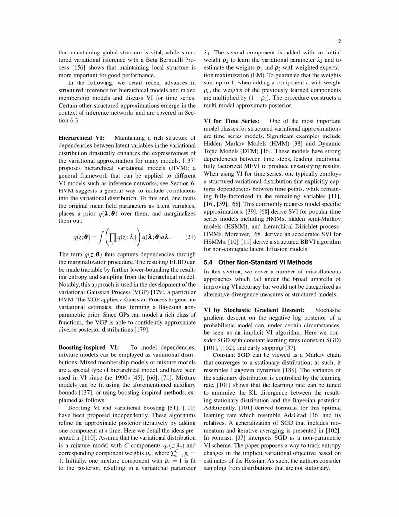
Hierarchical VI: Maintaining a rich structure ofdependencies between latent variables in the variationaldistribution drastically enhances the expressiveness ofthe variational approximation for many models. [137]proposes hierarchical variational models (HVM): ageneral framework that can be applied to differentVI models such as inference networks, see Section 6.HVM suggests a general way to include correlationsinto the variational distribution. To this end, one treatsthe original mean field parameters as latent variables,places a prior q(λλλ ;θθθ) over them, and marginalizesthem out:

q(zzz;θθθ) =∫ (

∏i

q(zi;λi)

)q(λλλ ;θθθ)dλλλ . (21)

The term q(zzz;θθθ) thus captures dependencies throughthe marginalization procedure. The resulting ELBO canbe made tractable by further lower-bounding the result-ing entropy and sampling from the hierarchical model.Notably, this approach is used in the development of thevariational Gaussian Process (VGP) [179], a particularHVM. The VGP applies a Gaussian Process to generatevariational estimates, thus forming a Bayesian non-parametric prior. Since GPs can model a rich class offunctions, the VGP is able to confidently approximatediverse posterior distributions [179].

Boosting-inspired VI: To model dependencies,mixture models can be employed as variational distri-butions. Mixed membership models or mixture modelsare a special type of hierarchical model, and have beenused in VI since the 1990s [45], [66], [71]. Mixturemodels can be fit using the aforementioned auxiliarybounds [137], or using boosting-inspired methods, ex-plained as follows.

Boosting VI and variational boosting [51], [110]have been proposed independently. These algorithmsrefine the approximate posterior iteratively by addingone component at a time. Here we detail the ideas pre-sented in [110]. Assume that the variational distributionis a mixture model with C components qc(z;λc) andcorresponding component weights ρc, where ∑

Cc=1 ρc =

1. Initially, one mixture component with ρc = 1 is fitto the posterior, resulting in a variational parameter

λ1. The second component is added with an initialweight ρ2 to learn the variational parameter λ2 and toestimate the weights ρ1 and ρ2 with weighted expecta-tion maximization (EM). To guarantee that the weightssum up to 1, when adding a component c with weightρc, the weights of the previously learned componentsare multiplied by (1−ρc). The procedure constructs amulti-modal approximate posterior.

VI for Time Series: One of the most importantmodel classes for structured variational approximationsare time series models. Significant examples includeHidden Markov Models (HMM) [38] and DynamicTopic Models (DTM) [16]. These models have strongdependencies between time steps, leading traditionalfully factorized MFVI to produce unsatisfying results.When using VI for time series, one typically employsa structured variational distribution that explicitly cap-tures dependencies between time points, while remain-ing fully-factorized in the remaining variables [11],[16], [39], [68]. This commonly requires model specificapproximations. [39], [68] derive SVI for popular timeseries models including HMMs, hidden semi-Markovmodels (HSMM), and hierarchical Dirichlet process-HMMs. Moreover, [68] derived an accelerated SVI forHSMMs. [10], [11] derive a structured BBVI algorithmfor non-conjugate latent diffusion models.

5.4 Other Non-Standard VI MethodsIn this section, we cover a number of miscellaneousapproaches which fall under the broad umbrella ofimproving VI accuracy but would not be categorized asalternative divergence measures or structured models.

VI by Stochastic Gradient Descent: Stochasticgradient descent on the negative log posterior of aprobabilistic model can, under certain circumstances,be seen as an implicit VI algorithm. Here we con-sider SGD with constant learning rates (constant SGD)[101], [102], and early stopping [37].

Constant SGD can be viewed as a Markov chainthat converges to a stationary distribution; as such, itresembles Langevin dynamics [188]. The variance ofthe stationary distribution is controlled by the learningrate. [101] shows that the learning rate can be tunedto minimize the KL divergence between the result-ing stationary distribution and the Bayesian posterior.Additionally, [101] derived formulas for this optimallearning rate which resemble AdaGrad [36] and itsrelatives. A generalization of SGD that includes mo-mentum and iterative averaging is presented in [102].In contrast, [37] interprets SGD as a non-parametricVI scheme. The paper proposes a way to track entropychanges in the implicit variational objective based onestimates of the Hessian. As such, the authors considersampling from distributions that are not stationary.

13

Robustness to Outliers and Local Optima: VI canbenefit from advanced optimization methods, whichaim to robustly escape to local optima. Variationaltempering [103] adapts an efficient annealing approach[121], [145] to VI. It anneals the likelihood term withan adaptive tempering rate which can be applied eitherglobally or locally to individual data points. Data pointswith associated small likelihoods under the model(such as outliers) are automatically assigned a hightemperature. This reduces their influence on the globalvariational parameters, making the inference algorithmmore robust to local optima. The same method can alsobe interpreted as data re-weighting [187], the weightbeing the inverse temperature. In this context, lowerweights are assigned to outliers. Other stabilizationtechniques of note include the trust-region method[168], which uses the KL divergence to regulate thechange between updating steps, and population VI[85], which uses bootstrapped populations to increasepredictive performance.

6 AMORTIZED VARIATIONAL INFERENCEAND DEEP LEARNING

Finally, we review amoritzed variational inference.Traditional VI with local latent variables makes itnecessary to optimize a separate variational parameterfor each data point; this is computationally expensive.Amortized VI circumvents this problem by learning adeterministic function from the data to distributionsover latent random variables. This replaces the locallatent variables by the globally shared parameters ofthe function. In this section, we detail the main ideasbehind this approach in Section 6.1 and how it isapplied in form of variational autoencoders in Sections6.2 and 6.3.

6.1 Amortized Variational InferenceThe term amortized inference refers to utilizing infer-ences from past computations to support future com-putations [44]. For VI, amortized inference usuallyrefers to inference over local variables. Instead ofapproximating separate variables for each data point,amortized VI assumes that these latent variables can bepredicted by a parameterized function of the data. Thus,once this function is estimated, the latent variables canbe acquired by passing new data points through thefunction. Deep neural networks used in this context arealso called inference networks. Amortised VI with in-ference networks thus combines probabilistic modelingwith the representational power of deep learning.

As an example, amortized inference has been ap-plied to Deep Gaussian Processes (DGPs) [30]. In-ference in these models is intractable, which is whythe authors apply MFVI with inducing points (seeSection 3.3) [30]. Instead of estimating these latent

θφ Z

X

(a) VAE

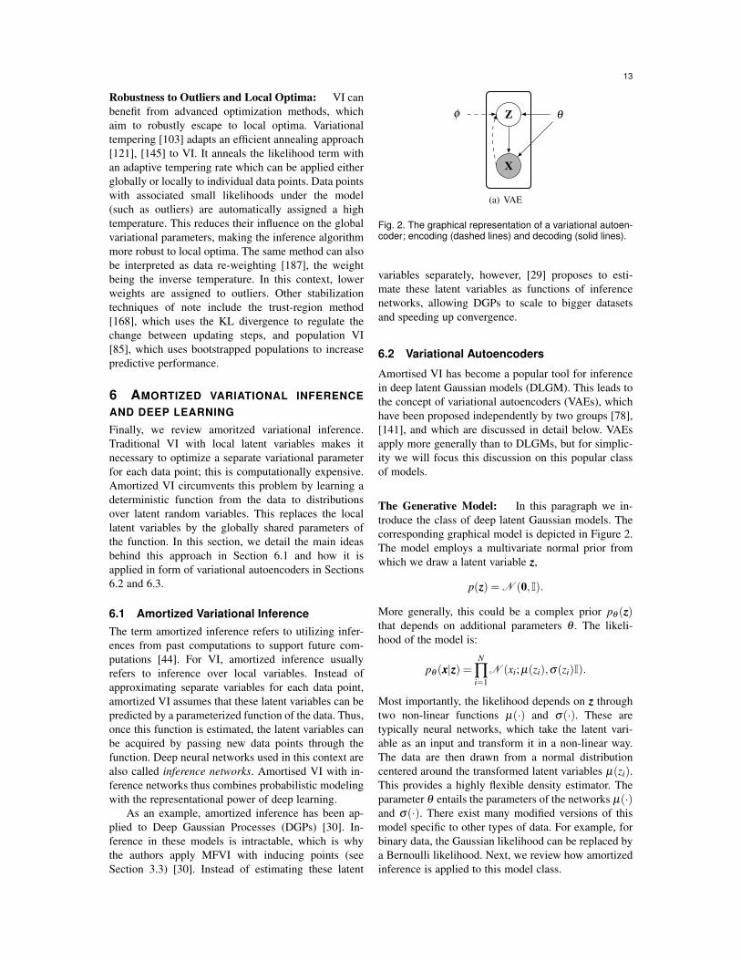
Fig. 2. The graphical representation of a variational autoen-coder; encoding (dashed lines) and decoding (solid lines).

variables separately, however, [29] proposes to esti-mate these latent variables as functions of inferencenetworks, allowing DGPs to scale to bigger datasetsand speeding up convergence.

6.2 Variational Autoencoders

Amortised VI has become a popular tool for inferencein deep latent Gaussian models (DLGM). This leads tothe concept of variational autoencoders (VAEs), whichhave been proposed independently by two groups [78],[141], and which are discussed in detail below. VAEsapply more generally than to DLGMs, but for simplic-ity we will focus this discussion on this popular classof models.

The Generative Model: In this paragraph we in-troduce the class of deep latent Gaussian models. Thecorresponding graphical model is depicted in Figure 2.The model employs a multivariate normal prior fromwhich we draw a latent variable zzz,

p(zzz) = N (0,I).

More generally, this could be a complex prior pθ (zzz)that depends on additional parameters θ . The likeli-hood of the model is:

pθ (xxx|zzz) =N

∏i=1

N (xi; µ(zi),σ(zi)I).

Most importantly, the likelihood depends on zzz throughtwo non-linear functions µ(·) and σ(·). These aretypically neural networks, which take the latent vari-able as an input and transform it in a non-linear way.The data are then drawn from a normal distributioncentered around the transformed latent variables µ(zi).This provides a highly flexible density estimator. Theparameter θ entails the parameters of the networks µ(·)and σ(·). There exist many modified versions of thismodel specific to other types of data. For example, forbinary data, the Gaussian likelihood can be replaced bya Bernoulli likelihood. Next, we review how amortizedinference is applied to this model class.

14

Variational Autoencoders: Most commonly, VAEsrefer to deep latent variable models which are trainedusing inference networks.

VAEs employ two deep sets of neural networks: atop-down generative model as described above, map-ping from the latent variables zzz to the data xxx, anda bottom-up inference model which approximates theposterior of the p(zzz|xxx). Commonly, these are referred toas the generative network and the recognition network.

In order to approximate the posterior, VAEs employan amortized variational distribution as follows:

qφ (zzz|xxx) =N

∏i=1

qφ (zi|xi).

As usual in amortized inference, this distribution doesnot depend on local variational parameters, but is in-stead conditioned on the data xi and is parametrizedby global parameters φ . This amortized variationaldistribution is typically chosen as:

qφ (zi|xi) = N (zi|µ(xi),σ2(xi)I). (22)

Similar to the generative model, the variational distri-bution employs non-linear mappings µ(xi) and σ(xi)of the data in order to predict the posterior distributionof xi. The parameter φ summarizes the correspondingneural network parameters.

The main contribution of [78], [141] was to derivea scalable and efficient training scheme for deep latentvariable models. During optimization, both the infer-ence network and the generative network are trainedjointly to optimize the ELBO. The key to training thesemodels is the reparameterization trick (see Section 4.3).

Stochastic gradients for the model’s ELBO canbe obtained as follows. One draws L local variablesamples ε(l) ∼ p(ε) with l = 1 : L, to build the ELBO’sMonte-Carlo approximation:

L (θ ,φ ,xi) =−DKL(qφ (z|xi)||pθ (z)) (23)

+1L

L

∑l=1

log pθ (xi|g(ε(l),µ(xi),σ2(xi))).

One uses the reparameterization trick, Eq. 23 to obtainstochastic gradients with respect to θ and φ .

The reparameterization trick also implies that thegradient variance is bounded by a constant [141]. Thedrawback of this approach however is that we requirethe posterior to be reparameterizable.

A Probabilistic Encoder-decoder Perspective:The term variational autoencoder arises from the factthat the joint training of the generative and recognitionnetwork resembles the structure of autoencoders, aclass of unsupervised, deterministic models. Autoen-coders are deep neural networks that are optimized toreconstruct their input xxx as closely as possible. Impor-tantly, autoencoders have a hourglass structure which

forces the information of the input to be compressedand filtered through a small number of units in theinner layers. These layers are thought to learn a low-dimensional manifold of the data.

In comparison, VAEs assume the low-dimensionalrepresentation of the data, the hidden variables zzz, to berandom variables and assign prior distributions to them.Thus, instead of a deterministic autoencoder, VAEslearn a probabilistic encoder and decoder which mapbetween the data density and the latent variables.

A technical difference between variational and de-terministic autoencoders is whether or not we injectnoise into the stochastic layer during training. This canbe thought of as a kind of regularization that avoidsover-fitting.

6.3 Advancements in VAEsSince the proposal of VAEs, an ever-growing numberof extensions have been proposed.

While exhaustive coverage of the topic would re-quire a review article in its own right, we summarize afew important extensions, including more expressivemodels and improved posterior inference. We alsoaddress specific problems of VAEs, such as the dyingunits problem.

More Expressive Likelihoods: One drawback ofthe standard VAE is the assumption that the like-lihood factorizes over dimensions. This can be apoor approximation for images. In order to achieve amore expressive decoder, the Deep Recurrent Atten-tive Writer [49] relies on a recurrent structure thatgradually constructs the observations while automat-ically focusing on regions of interest. In compari-son, PixelVAE [50] tackles this problem by modelingdependencies between pixels within an image, usingpθ (xi|zi) = ∏ j pθ (x

ji |x1

i , ...xj−1i ,zi), where x j

i denotesthe jth dimension of observation i. The dimensions aregenerated in a sequential fashion, which accounts forlocal dependencies.

More Expressive Posteriors: Just as in other mod-els, the mean field approach to VAEs suffers from alack of expressiveness to model a complex posterior.This can be overcome by loosening the standard mod-eling assumptions of the inference network, such as themean field assumption.

In order to tighten the variational bound, impor-tance weighted variational autoencoders (IWAE) havebeen proposed [21]. IWAEs require L samples from theapproximate posterior which are weighted by the ratio:

wl =wl

∑Ll=1 wl

,where wl =pθ (xi,z(i,l))qφ (z(i,l)|xi)

. (24)

A reinterpretation of IWAEs suggests that they areidentical to VAEs but sample from a more expressive,

15

implicit distribution which converges to the true poste-rior as L→ ∞ [26].

The expressiveness of the posterior is also ad-dressed in a series of papers on normalizing flows[25], [34], [35], [140] and [76]. The main idea behindnormalizing flows is to transform a simple (e.g. meanfield) approximate posterior q(z) into a more expressiveone by a series of successive invertible transformations.To this end, we first draw a random variable z ∼ q(z),and transform it using an invertible, smooth function f .Let z′ = f (z). Then the new distribution q(z′) is

q(z′) = q(z)|∂ f−1

∂ z′|= q(z)| ∂ f

∂ z′|−1. (25)

It is important that we can compute the determinantsince the variational approach requires us to alsoestimate the entropy of the transformed distribution.By choosing the function f such that | ∂ f

∂ z′ | is eas-ily computable, this normalizing flow constitutes anefficient method to generate multimodal distributionsfrom a simple distribution. To this end, linear time-transformations, Langevin and Hamilton flow [140], aswell as inverse autoregressive flow [76] and autoregres-sive flow [25] have been proposed.

The Dying Units Problem: While advances inposterior modeling are promising, VAEs can sufferfrom the optimization challenges that these modelsimpose. The expressiveness of the decoder can, in somecases, be so strong, that the optimization ignores thelatent code in the zzz variables. On one hand, this mightbe partly caused by the fact that the approximatingposterior does not carry relevant information in theearly stages of the optimization [18]. On the other hand,the decoder might be strong enough to model pθ (x|z)independent of z in which case the true posterior is theprior [25]. In these cases, the posterior is set to matchthe prior in order to satisfy the KL divergence in Eq.23. Lossy variational autoencoders [25] circumvent thisproblem by condititioning the decoding distribution foreach output dimension on partial input information.This forces the distribution to encode global informa-tion in the latent variables. A different approach is toapply an annealing scheme and slowly increase the in-fluence of the prior, i.e. the KL divergence term, duringtraining [159]. Furthermore, the generative distributioncan be corrected by recursively adjusting it with a datadependent approximate likelihood term [158].

Inference Networks and Graphical Models: In-stead of only relying on a neural network structure,[69] proposes a method to utilize a structured prior forVAEs. In this way, one combines the advantages oftraditional graphical models and inference networks.

These hybrid models overcome the intractabilityof non-conjugate likelihood distributions by learning

variational parameters of conjugate distributions with arecognition model. This allows one to approximate theposterior conditioned on the observations while main-taining conjugacy. As the encoder outputs an estimateof natural parameters, message passing, which relieson conjugacy, is applied to carry out the remaininginference.

Implicit Distributions: Traditional VI, includingVAEs, relies on parametric models. This facilitatesderivations and computations, but also limits our abilityto model complex data. One way to enhance expres-siveness is to employ implicit distributions. These aredistributions generated by a deterministic or stochastictransformation of another, possibly simpler distribu-tion. Implicit distributions do not have a parametriclikelihood function (preventing us from having accessto their entropy), but we can still sample from them,which is often enough to estimate the desired gradients.One popular example is to use Generative AdversarialNetworks (GAN) [48] which learn implicit distribu-tions to represent unknown densities.

Several authors have proposed implicit distributionsfor amortized inference [64], [73], [93], [105], [115].When employing an implicit distribution as a varia-tional distribution in VAEs, the standard training proce-dure does not apply because the entropy is intractable.Instead, a GAN-style discriminator can be trained todistinguish between the target distribution and thevariational distribution [105]. As part of VI, we aimto approximate an expectation of the log density ratiolog p(zzz)− logqφ (zzz|xxx) under q. employ a GAN-stylediscriminator T that discriminates the prior from thevariational distribution, T (xxx,zzz) = logqφ (zzz|xxx)− log p(zzz)[105].

7 DISCUSSION

We have summarized recent advancements in varia-tional inference. Here we outline some selected activeresearch directions and open questions, including, butnot limited to: theory of VI, VI and policy gradients,VI for deep learning (DL), and automatic VI.

Theory of VI: Despite progress in modeling andinference, few authors address theoretical aspects ofVI. One important direction is quantifying the approx-imation errors involved when replacing a true poste-rior with a simplified variational distribution [118]. Arelated problem is the predictive error, e.g., when ap-proximating the marginalization involved in a Bayesianpredictive distribution using VI.

We also conjecture that VI theory could profitfrom a deeper connection with information theory. Thiswas already exemplified in [165], [166]. Informationtheory also inspires the development of new models

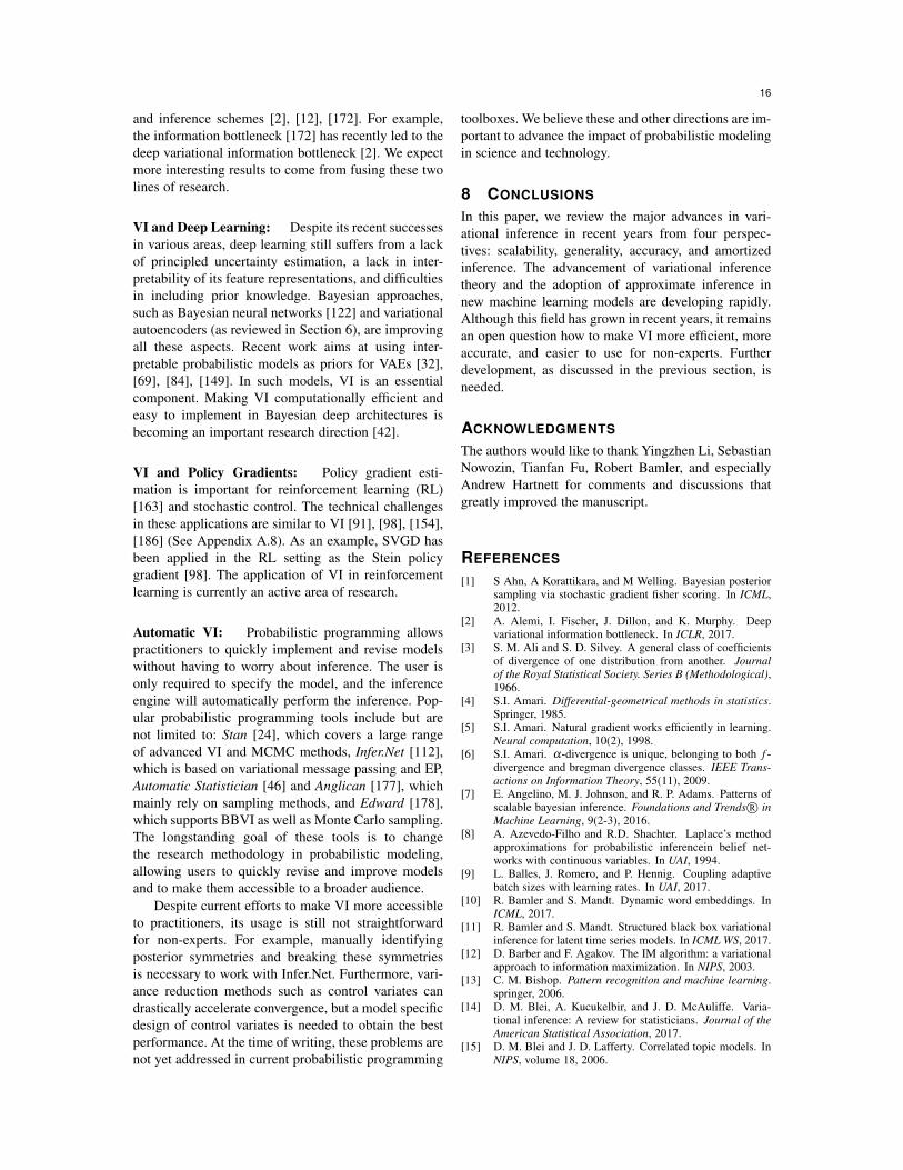
16

and inference schemes [2], [12], [172]. For example,the information bottleneck [172] has recently led to thedeep variational information bottleneck [2]. We expectmore interesting results to come from fusing these twolines of research.

VI and Deep Learning: Despite its recent successesin various areas, deep learning still suffers from a lackof principled uncertainty estimation, a lack in inter-pretability of its feature representations, and difficultiesin including prior knowledge. Bayesian approaches,such as Bayesian neural networks [122] and variationalautoencoders (as reviewed in Section 6), are improvingall these aspects. Recent work aims at using inter-pretable probabilistic models as priors for VAEs [32],[69], [84], [149]. In such models, VI is an essentialcomponent. Making VI computationally efficient andeasy to implement in Bayesian deep architectures isbecoming an important research direction [42].

VI and Policy Gradients: Policy gradient esti-mation is important for reinforcement learning (RL)[163] and stochastic control. The technical challengesin these applications are similar to VI [91], [98], [154],[186] (See Appendix A.8). As an example, SVGD hasbeen applied in the RL setting as the Stein policygradient [98]. The application of VI in reinforcementlearning is currently an active area of research.

Automatic VI: Probabilistic programming allowspractitioners to quickly implement and revise modelswithout having to worry about inference. The user isonly required to specify the model, and the inferenceengine will automatically perform the inference. Pop-ular probabilistic programming tools include but arenot limited to: Stan [24], which covers a large rangeof advanced VI and MCMC methods, Infer.Net [112],which is based on variational message passing and EP,Automatic Statistician [46] and Anglican [177], whichmainly rely on sampling methods, and Edward [178],which supports BBVI as well as Monte Carlo sampling.The longstanding goal of these tools is to changethe research methodology in probabilistic modeling,allowing users to quickly revise and improve modelsand to make them accessible to a broader audience.

Despite current efforts to make VI more accessibleto practitioners, its usage is still not straightforwardfor non-experts. For example, manually identifyingposterior symmetries and breaking these symmetriesis necessary to work with Infer.Net. Furthermore, vari-ance reduction methods such as control variates candrastically accelerate convergence, but a model specificdesign of control variates is needed to obtain the bestperformance. At the time of writing, these problems arenot yet addressed in current probabilistic programming

toolboxes. We believe these and other directions are im-portant to advance the impact of probabilistic modelingin science and technology.

8 CONCLUSIONS

In this paper, we review the major advances in vari-ational inference in recent years from four perspec-tives: scalability, generality, accuracy, and amortizedinference. The advancement of variational inferencetheory and the adoption of approximate inference innew machine learning models are developing rapidly.Although this field has grown in recent years, it remainsan open question how to make VI more efficient, moreaccurate, and easier to use for non-experts. Furtherdevelopment, as discussed in the previous section, isneeded.

ACKNOWLEDGMENTS

The authors would like to thank Yingzhen Li, SebastianNowozin, Tianfan Fu, Robert Bamler, and especiallyAndrew Hartnett for comments and discussions thatgreatly improved the manuscript.

REFERENCES

[1] S Ahn, A Korattikara, and M Welling. Bayesian posteriorsampling via stochastic gradient fisher scoring. In ICML,2012.

[2] A. Alemi, I. Fischer, J. Dillon, and K. Murphy. Deepvariational information bottleneck. In ICLR, 2017.

[3] S. M. Ali and S. D. Silvey. A general class of coefficientsof divergence of one distribution from another. Journalof the Royal Statistical Society. Series B (Methodological),1966.

[4] S.I. Amari. Differential-geometrical methods in statistics.Springer, 1985.

[5] S.I. Amari. Natural gradient works efficiently in learning.Neural computation, 10(2), 1998.

[6] S.I. Amari. α-divergence is unique, belonging to both f -divergence and bregman divergence classes. IEEE Trans-actions on Information Theory, 55(11), 2009.

[7] E. Angelino, M. J. Johnson, and R. P. Adams. Patterns ofscalable bayesian inference. Foundations and Trends R© inMachine Learning, 9(2-3), 2016.

[8] A. Azevedo-Filho and R.D. Shachter. Laplace’s methodapproximations for probabilistic inferencein belief net-works with continuous variables. In UAI, 1994.

[9] L. Balles, J. Romero, and P. Hennig. Coupling adaptivebatch sizes with learning rates. In UAI, 2017.

[10] R. Bamler and S. Mandt. Dynamic word embeddings. InICML, 2017.

[11] R. Bamler and S. Mandt. Structured black box variationalinference for latent time series models. In ICML WS, 2017.

[12] D. Barber and F. Agakov. The IM algorithm: a variationalapproach to information maximization. In NIPS, 2003.

[13] C. M. Bishop. Pattern recognition and machine learning.springer, 2006.

[14] D. M. Blei, A. Kucukelbir, and J. D. McAuliffe. Varia-tional inference: A review for statisticians. Journal of theAmerican Statistical Association, 2017.

[15] D. M. Blei and J. D. Lafferty. Correlated topic models. InNIPS, volume 18, 2006.

17

[16] D. M. Blei and J. D. Lafferty. Dynamic topic models. InICML, 2006.

[17] L. Bottou. Large-scale machine learning with stochasticgradient descent. Springer, 2010.

[18] S. R. Bowman, L. Vilnis, O. Vinyals, A. M. Dai,R. Jozefowicz, and S. Bengio. Generating sentences froma continuous space. In CoNLL, pages 10–21, 2016.

[19] S. Brooks, A. Gelman, G. Jones, and X.L Meng. Handbookof markov chain monte carlo. CRC press, 2011.

[20] T. D. Bui, J. Yan, and R. E. Turner. A unifying frameworkfor sparse gaussian process approximation using power ex-pectation propagation. arXiv preprint arXiv:1605.07066,2016.

[21] Y. Burda, R. Grosse, and R. Salakhutdinov. Importanceweighted autoencoders. arXiv preprint arXiv:1509.00519,2015.

[22] R.H. Byrd, G.M. Chin, J. Nocedal, and Y.C. Wu. Soam-ploample size selection in optimization methods for ma-chine learning. Mathematical programming, 134(1), 2012.

[23] L. Le Cam. Asymptotic methods in statistical decisiontheory. Springer Science & Business Media, 2012.

[24] B. Carpenter, D. Lee, M. A. Brubaker, A. Riddell, A. Gel-man, B. Goodrich, J. Guo, M. Hoffman, M. Betancourt,and P Li. Stan: A probabilistic programming language.Journal of Statistical Software, 2016.

[25] X. Chen, D. P. Kingma, T. Salimans, Y. Dua, P. Dhariwal,J. Schulman, I. Sutskever, and P. Abbeel. Variational lossyautoencoder. In ICLR, 2017.

[26] C. Cremer, Q. Morris, and D. Duvenaud. Reinterpretingimportance-weighted autoencoders. In ICLR WS, 2017.

[27] D. Csiba and P. Richtarik. Importance sampling forminibatches. arXiv preprint arXiv:1602.02283, 2016.

[28] I. Csiszar. Eine informationstheoretische ungleichung undihre anwendung auf beweis der ergodizitaet von markoff-schen ketten. Magyer Tud. Akad. Mat. Kutato Int. Koezl.,8, 1964.

[29] Z.W. Dai, A. Damianou, J. Gonzalez, and N. Lawrence.Variational auto-encoded deep Gaussian processes. InICLR, 2016.

[30] A. Damianou and N. Lawrence. Deep gaussian processes.In AISTATS, 2013.

[31] S. De, A. Yadav, D. Jacobs, and T. Goldstein. Automatedinference using adaptive batch sizes. In AISTATS, 2017.

[32] Z.W. Deng, R. Navarathna, P. Carr, S. Mandt, Y.S. Yue,I. Matthews, and G. Mori. Factorized variational autoen-coders for modeling audience reactions to movies. InCVPR, 2017.

[33] A. B. Dieng, D. Tran, R. Ranganath, J. Paisley, andD. M. Blei. Variational inference via chi-upper boundminimization. In NIPS, 2017.

[34] L. Dinh, D. Krueger, and Y. Bengio. NICE: non-linear independent components estimation. arXiv preprintarXiv:1410.8516, 2014.

[35] L. Dinh, J. Sohl-Dickstein, and S. Bengio. Density estima-tion using real nvp. In ICLR, 2017.

[36] J. Duchi, E. Hazan, and Y. Singer. Adaptive subgradientmethods for online learning and stochastic optimization.JMLR, 12, 2011.

[37] D. Duvenaud, D. Maclaurin, and R. Adams. Early stoppingas nonparametric variational inference. In AISTATS, 2016.

[38] S. R. Eddy. Hidden Markov Models. Current opinion instructural biology, 6(3), 1996.

[39] N. Foti, J. Xu, D. Laird, and E. Fox. Stochastic variationalinference for hidden Markov models. In NIPS, 2014.

[40] M. P. Friedlander and M. Schmidt. Hybrid deterministic-stochastic methods for data fitting. SIAM Journal onScientific Computing, 34(3), 2012.

[41] T.F Fu and Z.H. Zhang. CPSG-MCMC: Clustering-basedpreprocessing method for stochastic gradient mcmc. InAISTATS, 2017.

[42] Y. Gal. Uncertainty in deep learning. PhD thesis, PhDthesis, University of Cambridge, 2016.

[43] Y. Gal, M. van der Wilk, and C. Rasmussen. Distributedvariational inference in sparse gaussian process regressionand latent variable models. In NIPS, 2014.

[44] S. Gershman and N. Goodman. Amortized inference inprobabilistic reasoning. In CogSci, volume 36, 2014.

[45] S. J. Gershman, M. D. Hoffman, and D. M. Blei. Nonpara-metric variational inference. In ICML, 2012.

[46] Z. Ghahramani. Probabilistic Machine Learning and Arti-ficial Intelligence. Nature, 521(7553), 2015.

[47] I. Goodfellow, Y. Bengio, and A. Courville. Deep Learn-ing. MIT Press, 2016.

[48] I. Goodfellow, J. Pouget-Abadie, M. Mirza, B. Xuand D.Warde-Farley, S. Ozair, A. Courville, and Y. Bengio. Gen-erative adversarial nets. In NIPS, 2014.

[49] K. Gregor, I. Danihelka, A. Graves, D. J. Rezende, andD. Wierstra. Draw: A recurrent neural network for imagegeneration. In ICML, 2015.

[50] I. Gulrajani, K. Kumar, F. Ahmed, A. A. Taiga, F. V. Visin,D. Vazquez, and A. Courville. PixelVAE: A latent variablemodel for natural images. 2017.

[51] F.J. Guo, X.Y. Wang, K. Fan, T. Broderick, and D. B.Dunson. Boosting variational inference. arXiv preprintarXiv:1611.05559, 2016.

[52] J. Han and Q. Liu. Stein variational adaptive importancesampling. In UAI, 2017.

[53] G. Heinrich. Parameter estimation for text analysis, 2008.[54] P. Hennig. Approximate inference in graphical models.

PhD thesis, University of Cambridge, 2011.[55] J. Hensman, N. Fusi, and N. D. Lawrence. Gaussian

processes for big data. In UAI, 2013.[56] J Hensman, M Rattray, and N. D Lawrence. Fast varia-

tional inference in the conjugate exponential family. InNIPS, 2012.

[57] M. Hoffman, F. R. Bach, and D. M. Blei. Online learningfor Latent Dirichlet Allocation. In NIPS, 2010.

[58] M. D. Hoffman and D. M. Blei. Structured stochasticvariational inference. In AISTATS, 2015.

[59] M D. Hoffman, D. M. Blei, C. Wang, and J. Paisley.Stochastic variational inference. JMLR, 14(1), 2013.

[60] R. V. Hogg and A. T. Craig. Introduction to mathematicalstatistics.(5th edition). Upper Saddle River, New Jersey:Prentice Hall, 1995.

[61] A. Honkela, T. Raiko, M. Kuusela, M. Tornio, andJ. Karhunen. Approximate riemannian conjugate gradientlearning for fixed-form variational bayes. JMLR, 11(Nov),2010.

[62] A. Honkela, M. Tornio, T. Raiko, and J. Karhunen. Naturalconjugate gradient in variational inference. In ICONIP,pages 305–314, 2007.

[63] A. Honkela and H. Valpola. Online variational bayesianlearning. In International Symposium on IndependentComponent Analysis and Blind Signal Separation, 2003.

[64] F. Huszar. Variational inference using implicit distribu-tions. arXiv preprint arXiv:1702.08235, 2017.

[65] T. S. Jaakkol, L. K. Saul, and M. I. Jordan. Fast learningby bounding likelihoods in sigmoid type belief networks.NIPS, 1996.

[66] T. S. Jaakkola and M. I. Jordan. Improving the mean fieldapproximation via the use of mixture distributions. NATOASI series D behaviroural and social sciences, 89, 1998.

[67] E. Jang, S.X. Gu, and B. Poole. Categorical reparameteri-zation with gumbel-softmax. In ICLR, 2017.

[68] M. Johnson and A. Willsky. Stochastic variational infer-ence for bayesian time series models. In ICML, 2014.

[69] M. J. Johnson, D. Duvenaud, A. B. Wiltschko, S. R. Datta,and R. P. Adams. Structured VAEs: Composing proba-bilistic graphical models and variational autoencoders. InNIPS, 2016.

18

[70] R. Johnson and T. Zhang. Accelerating stochastic gradientdescent using predictive variance reduction. In NIPS, 2013.

[71] M. I. Jordan, Z. Ghahramani, T. S. Jaakkola, and L. K.Saul. An introduction to variational methods for graphicalmodels. Machine learning, 37(2), 1999.

[72] H. J. Kappen and W. Wiegerinck. Second order approxi-mations for probability models. In NIPS, 2001.

[73] T. Karaletsos. Adversarial message passing for graphicalmodels. In NIPS WS. 2016.

[74] M. E. Khan, P. Baque, F. Fleuret, and P. Fua. Kullback-Leibler Proximal Variational Inference. In NIPS, 2015.

[75] N. King and N. Lawrence. Fast variational inference forgaussian process models through kl-correction. In ECML.Springer, 2006.

[76] D. P. Kingma, T. Salimans, R. Jozefowicz, X. Chen,I. Sutskever, and M. Welling. Improving variationalautoencoders with inverse autoregressive flow. In NIPS,2016.

[77] D. P. Kingma, T. Salimans, and M. Welling. VariationalDropout and the Local Reparameterization Trick. In NIPS,2015.

[78] D. P. Kingma and M. Welling. Auto-encoding variationalbayes. In ICLR, 2014.

[79] D. P. Kingma and M. Welling. Stochastic gradient vb andthe variational auto-encoder. In ICLR, 2014.

[80] D.P. Kingma and J. Ba. Adam: A method for stochasticoptimization. In ICLR, 2015.

[81] D. A. Knowles and T. P. Minka. Non-conjugate variationalmessage passing for multinomial and binary regression. InNIPS, 2011.

[82] D.A. Knowles. Stochastic gradient variational Bayesfor gamma approximating distributions. arXiv, page1509.01631, 2015.

[83] A. Korattikara, V. Rathod, K. Murphy, andM. Welling. Bayesian Dark Knowledge. arXiv preprintarXiv:1506.04416, 2015.

[84] R. G. Krishnan, U. Shalit, and D. Sontag. Deep kalmanfilters. In NIPS WS, 2015.

[85] A. Kucukelbir and D. M. Blei. Population empirical bayes.In UAI, 2015.

[86] A. Kulesza and B. Taskar. Determinantal point processesfor machine learning. Foundations and Trends R© in Ma-chine Learning, 5(2–3):123–286, 2012.

[87] S. Kullback and R. A. Leibler. On information andsufficiency. The annals of mathematical statistics, 22(1),1951.

[88] K. Kurihara, M. Welling, and Y. W. Teh. Collapsedvariational dirichlet process mixture models. In IJCAI,2007.

[89] P. S. Laplace. Memoir on the probability of the causes ofevents. Statistical Science, 1(3), 1986.

[90] M. Lazaro-Gredilla, S. Van Vaerenbergh, and N. D.Lawrence. Overlapping mixtures of gaussian processes forthe data association problem. Pattern Recognition, 45(4),2012.

[91] S. Levine and V. Koltun. Variational policy search viatrajectory optimization. In NIPS, 2013.

[92] Y.Z. Li, J.M. Hernandez-Lobato, and R.E. Turner. Stochas-tic expectation propagation. In NIPS, 2015.

[93] Y.Z. Li and Q. Liu. Wild variational approximations. InNIPS WS, 2016.

[94] Y.Z Li and r. e. Turner. Renyi divergence variationalinference. In NIPS, 2016.

[95] Y.Z Li, M. Rowland, T. Bui, D. Hernandez-Lobato, andR. Turner. Black-Box Alpha Divergence Minimization. InICML, 2016.

[96] Q. Liu, J. Lee, and M. Jordan. A kernelized stein discrep-ancy for goodness-of-fit tests. In ICML, 2016.

[97] Q. Liu and D. Wang. Stein variational gradient descent:A general purpose bayesian inference algorithm. In NIPS,2016.

[98] Y. Liu, P. Ramachandran, Q. Liu, and J. Peng. Steinvariational policy gradient. In UAI, 2017.

[99] C. J. Maddison, A. Mnih, and Y. W. Teh. The concretedistribution: A continuous relaxation of discrete randomvariables, 2017.

[100] S. Mandt and D. Blei. Smoothed gradients for stochasticvariational inference. In NIPS, 2014.

[101] S. Mandt, M. D. Hoffman, and D. M. Blei. A VariationalAnalysis of Stochastic Gradient Algorithms. In ICML,2016.

[102] S. Mandt, M. D. Hoffman, and D. M. Blei. Stochastic gra-dient descent as approximate bayesian inference. JMLR,2017.

[103] S. Mandt, J. McInerney, F. Abrol, R. Ranganath, and Blei.Variational Tempering. In AISTATS, 2016.

[104] J. McInerney, R. Ranganath, and D. Blei. The populationposterior and bayesian modeling on streams. In NIPS,2015.

[105] L. Mescheder, S. Nowozin, and A. Geiger. Adversarialvariational bayes: Unifying variational autoencoders andgenerative adversarial networks. In ICML, 2017.

[106] L. Mescheder, S. Nowozin, and A. Geiger. The numericsof gans. In NIPS, 2017.

[107] M. Mezard, G. Parisi, and M. A. Virasoro. Spin glasstheory and beyond. 1990.

[108] Y. Miao, L. Yu, and P. Blunsom. Neural variationalinference for text processing. In ICML, 2016.

[109] A. C. Miller, N. J. Foti, A. D’Amour, and R. P. Adams.Reducing reparameterization gradient variance. In NIPS,2017.

[110] A.C. Miller, N. Foti, and R. P. Adams. Variationalboosting: Iteratively refining posterior approximations. InICML, 2017.

[111] T. Minka. Power EP. Technical report, Technical report,Microsoft Research, Cambridge, 2004.

[112] T. Minka, J. M. Winn, J. P. Guiver, S. Webster, Y. Zaykov,B. Yangel, A. Spengler, and J. Bronskill. Infer.NET 2.6.http://research.microsoft.com/infernet, 2014. MicrosoftResearch Cambridge.

[113] T. P. Minka. Expectation propagation for approximatebayesian inference. In UAI, 2001.

[114] T. P. Minka. Divergence measures and message passing.In Microsoft Research Technical Report, 2005.

[115] S. Mohamed and B. Lakshminarayanan. Learning in im-plicit generative models. arXiv preprint arXiv:1610.03483,2016.

[116] K. P. Murphy, Y. Weiss, and M. I. Jordan. Loopy be-lief propagation for approximate inference: An empiricalstudy. In UAI, 1999.

[117] C. Naesseth, F. Ruiz, S. Linderman, and D. M. Blei.Reparameterization gradients through acceptance-rejectionsampling algorithms. In AISTATS, 2017.

[118] S. Nakajima and S. Watanabe. Variational bayes solutionof linear neural networks and its generalization perfor-mance. Neural Computation, 19(4), 2007.

[119] Eric Nalisnick and Padhraic Smyth. Stick-breaking varia-tional autoencoders. In ICLR, 2017.

[120] R. Nallapati, W. Cohen, and J. Lafferty. Parallelized vari-ational em for latent dirichlet allocation: An experimentalevaluation of speed and scalability. In ICDM WS, 2007.

[121] R. M. Neal. Probabilistic inference using markov chainmonte carlo methods. In Technical Report, 1993.

[122] R. M. Neal. Bayesian learning for neural networks,volume 118. Springer Science & Business Media, 2012.

[123] W. Neiswanger, C. Wang, and E. Xing. Embarrassinglyparallel variational inference in nonconjugate models.arXiv preprint arXiv:1510.04163, 2015.

[124] M. Opper, M. Fraccaro, U. Paquet, A. Susemihl, andO. Winther. Perturbation theory for variational inference.NIPS WS, 2015.

19

[125] M. Opper, U. Paquet, and O. Winther. Perturbative correc-tions for approximate inference in gaussian latent variablemodels. JMLR, 14(1), 2013.

[126] M. Opper and D. Saad. Advanced mean field methods:Theory and practice. MIT press, 2001.

[127] M. Opper and O. Winther. A mean field algorithm forbayes learning in large feed-forward neural networks. InNIPS, 1996.

[128] M. Opper and O. Winther. Tractable approximationsfor probabilistic models: The adaptive thouless-anderson-palmer mean field approach. Physical Review Letters,86(17), 2001.

[129] J. Paisley, D. M. Blei, and M. I. Jordan. Variationalbayesian inference with stochastic search. In ICML, 2012.

[130] G. Parisi. Statistical field theory. Addison-Wesley, 1988.[131] D Perekrestenko, V Cevher, and M Jaggi. Faster coordinate

descent via adaptive importance sampling. In AISTATS,2017.

[132] C. Peterson and J. R. Anderson. A mean field theorylearning algorithm for neural networks. Complex systems,1, 1987.

[133] T Plefka. Convergence condition of the TAP equationfor the infinite-ranged ising spin glass model. Journal ofPhysics A: Mathematical and general, 15(6), 1982.

[134] I. Porteous, D. Newman, A. Ihler, A. Asuncion, P. Smyth,and M. Welling. Fast collapsed gibbs sampling for latentdirichlet allocation. 2008.

[135] R. Ranganath, S. Gerrish, and D. Blei. Black box varia-tional inference. In AISTATS, 2014.

[136] R. Ranganath, D. Tran, J. Altosaar, and D. M. Blei.Operator variational inference. In NIPS. 2016.

[137] R. Ranganath, D. Tran, and D. M. Blei. Hierarchicalvariational models. In ICML, 2016.

[138] R. Ranganath, C. Wang, D. Blei, and E. Xing. An adaptivelearning rate for Stochastic Variational Inference. In ICML,2013.

[139] J. Raymond, A. Manoel, and M. Opper. Expectationpropagation. arXiv preprint arXiv:1409.6179, 2014.

[140] D. Rezende and S. Mohamed. Variational Inference withNormalizing Flows. In ICML, 2015.

[141] D. J. Rezende, S. Mohamed, and D. Wierstra. Stochasticbackpropagation and approximate inference in deep gen-erative models. In ICML, 2014.

[142] B. Ringner. Law of the unconscious statistician. InUnpublished Notes, Lund University.

[143] H. Robbins and S. Monro. A stochastic approximationmethod. The annals of mathematical statistics, 1951.

[144] G. Roeder, Y. Wu, and D. Duvenaud. Sticking the landing:An asymptotically zero-variance gradient estimator forvariational inference. In NIPS, 2017.

[145] K. Rose, E. Gurewitz, and G. Fox. A deterministic anneal-ing approach to clustering. Pattern Recognition Letters,11(9), 1990.

[146] S. M. Ross. Simulation. Elsevier, 2006.[147] F. J.R. Ruiz, M. K. Titsias, and D. M. Blei. The generalized

reparameterization gradient. In NIPS. 2016.[148] F. J.R. Ruiz, M. K. Titsias, and D. M. Blei. Overdispersed

black-box variational inference. In UAI, 2016.[149] A. Saeedi, M. D. Hoffman, S. J. DiVerdi, A. Ghande-

harioun, M. J. Johnson, and R. P. Adams. Multimodalprediction and personalization of photo edits with deepgenerative models. arXiv preprint arXiv:1704.04997,2017.

[150] T. Salimans, D. P. Kingma, and M. Welling. Markov chainmonte carlo and variational inference: Bridging the gap. InICML, 2015.

[151] T. Salimans and D. A. Knowles. Fixed-form variationalposterior approximation through stochastic linear regres-sion. Bayesian Analysis, 8(4), 2013.

[152] M. Sato. Online model selection based on the variationalBayes. Neural Computation, 13(7):1649–1681, 2001.

[153] L. K. Saul, T. Jaakkola, and M. I. Jordan. Mean fieldtheory for sigmoid belief networks. Journal of artificialintelligence research, 4(1), 1996.

[154] J. Schulman, S. Levine, P. Abbeel, M. Jordan, andP. Moritz. Trust region policy optimization. In ICML,2015.

[155] M. Seeger. Expectation propagation for exponential fami-lies. Technical report, 2005.

[156] A. Shah, D. A. Knowles, and Z. Ghahramani. An Empiri-cal Study of Stochastic Variational Algorithms for the BetaBernoulli Process. In ICML, 2015.

[157] E. Snelson and Z. Ghahramani. Sparse gaussian processesusing pseudo-inputs. NIPS, 18, 2006.

[158] C. K. Sønderby, R. Raiko, L. Maaløe, S. Sønderby, andO. Winther. Ladder variational autoencoders. In NIPS,2016.

[159] C. K. Sønderby, T. Raiko, L. Maaløe, S. K. Sønderby, andO. Winther. How to train deep variational autoencodersand probabilistic ladder networks. In ICML, 2016.

[160] A. Srivastava and C. Sutton. Autoencoding variationalinference for topic models. In ICLR, 2017.

[161] C. Stein. A bound for the error in the normal approxi-mation to the distribution of a sum of dependent randomvariables. In Berkeley Symposium on Mathematical Statis-tics and Probability, 1972.

[162] J. Sung, Z. Ghahramani, and S. Y. Bang. Latent-spacevariational bayes. TPAMI, 30(12), 2008.

[163] R. S. Sutton and A. G. Barto. Reinforcement learning: Anintroduction, volume 1. MIT press Cambridge, 1998.

[164] T. Tanaka. Estimation of third-order correlations withinmean field approximation. In NIPS, 1998.

[165] T. Tanaka. A theory of mean field approximation. In NIPS,1999.

[166] T. Tanaka. Information geometry of mean-field approxi-mation. Neural Computation, 12(8), 2000.

[167] Y. W. Teh, D. Newman, and M. Welling. A collapsed vari-ational Bayesian inference algorithm for latent Dirichletallocation. In NIPS, 2006.

[168] L. Theis and M. Hoffman. A Trust-region Methodfor Stochastic Variational Inference with Applications toStreaming Data. In ICML, 2015.

[169] D.J. Thouless, P. W. Anderson, and R. G. Palmer. So-lution of ’solvable model of a spin glass’. PhilosophicalMagazine, 35(3), 1977.

[170] T. Tieleman and G. Hinton. Lecture 6.5-rmsprop: Dividethe gradient by a running average of its recent magnitude.COURSERA: Neural networks for machine learning, 4(2),2012.

[171] L. Tierney and J.B. Kadane. Accurate approximations forposterior moments and marginal densities. Journal of theamerican statistical association, 81(393), 1986.

[172] N. Tishby, F. C. Pereira, and W. Bialek. The informationbottleneck method. arXiv preprint physics/0004057, 2000.

[173] M. Titsias and M. Lazaro-Gredilla. Local ExpectationGradients for Black Box Variational Inference. In NIPS,2015.

[174] M. K. Titsias. Variational learning of inducing variables insparse gaussian processes. In AISTATS, 2009.

[175] M.K. Titsias and M. Lazaro-Gredilla. Variational het-eroscedastic gaussian process regression. In ICML, 2011.

[176] S. Tokui and I. Sato. Evaluating the variance of likelihood-ratio gradient estimators. In ICML, 2017.

[177] D. Tolpin, J. W. van de Meent, H. Yang, and F. Wood.Design and implementation of probabilistic programminglanguage anglican. arXiv preprint arXiv:1608.05263,2016.

[178] D. Tran, A. Kucukelbir, A. B. Dieng, M. Rudolph,D. Liang, and D. M. Blei. Edward: A library for prob-abilistic modeling, inference, and criticism. arXiv preprintarXiv:1610.09787, 2016.

20

[179] D. Tran, R. Ranganath, and D. M. Blei. The VariationalGaussian Process. stat, 1050, 2016.

[180] M. J. Wainwright, T. S. Jaakkola, and A. S. Willsky. Anew class of upper bounds on the log partition function.IEEE Transactions on Information Theory, 51(7), 2005.

[181] M. J. Wainwright and M. I. Jordan. Graphical models, ex-ponential families, and variational inference. Foundationsand Trends R© in Machine Learning, 1(1-2), 2008.

[182] C. Wang, D. Blei, and L. Fei-Fei. Simultaneous imageclassification and annotation. In CVPR, 2009.

[183] C. Wang and D. M. Blei. Variational inference in non-conjugate models. JMLR, 14(Apr), 2013.

[184] C. Wang, X. Chen, A. J. Smola, and E. P. Xing. Variancereduction for stochastic gradient optimization. In NIPS,2013.

[185] C. Wang, J. Paisley, and D. M. Blei. Online variational in-ference for the hierarchical dirichlet process. In AISTATS,2011.

[186] Y. Wang, G. Williams, E. Theodorou, and L. Song. Varia-tional policy for guiding point processes. In ICML, 2017.

[187] Y. X. Wang, A. Kucukelbir, and D. M. Blei. RobustProbabilistic Modeling with Bayesian Data Reweighting.In ICML, 2017.

[188] M. Welling and Y. W. Teh. Bayesian learning via stochasticgradient langevin dynamics. In ICML, 2011.

[189] R. J. Williams. Simple statistical gradient-following algo-rithms for connectionist reinforcement learning. Machinelearning, 8(3-4):229–256, 1992.

[190] J. Winn and C. M. Bishop. Variational message passing.JMLR, 6, 2005.

[191] M.D. Zeiler. Adadelta: an adaptive learning rate method.arXiv preprint arXiv:1212.5701, 2012.

[192] K. Zhai, J. Boyd-Graber, N. Asadi, and M. L. Alkhouja.Mr. lda: A flexible large scale topic modeling packageusing variational inference in mapreduce. In WWW, 2012.

[193] C. Zhang. Structured Representation Using Latent Vari-able Models. PhD thesis, KTH Royal Institute of Technol-ogy, 2016.

[194] C. Zhang, R. Bamler, M. Opper, and S. Mandt. Perturba-tive black box variational inference. In NIPS, 2017.

[195] C. Zhang, C. H. Ek, X. Gratal, F. T. Pokorny, and H. Kjell-strom. Supervised hierarchical Dirichlet processes withvariational inference. In ICCV WS, 2013.

[196] C. Zhang, H. Kjellstrom, and S. Mandt. Determinantalpoint processes for mini-batch diversification. In UAI,2017.

[197] P.L. Zhao and T. Zhang. Accelerating minibatch stochasticgradient descent using stratified sampling. arXiv preprintarXiv:1405.3080, 2014.

[198] P.L. Zhao and T. Zhang. Stochastic optimization withimportance sampling for regularized loss minimization. InICML, 2015.

[199] S.D. Zhe, K.C. Lee, K. Zhang, and J. Neville. Onlinespike-and-slab inference with stochastic expectation prop-agation. In NIPS WS, 2016.

[200] H. Zhu and R. Rohwer. Information geometric measure-ments of generalisation. Technical report, 1995.

Cheng Zhang obtained her mas-ter’s degree in System Control andRobotics from KTH Royal Instituteof Technology in fall 2011. Shereceived her Ph.D. degree at theDepartment of Robotics, Percep-tion, and Learning (RPL), KTH, Sep2016. She is currently a postdoc-toral research associate at DisneyResearch, Pittsburgh. Her researchinterest lies in probabilistic models

and approximate Bayesian inference, as well as their ap-plications in computer vision and health care.

Judith Butepage holds a Bsc de-gree in Cognitive Science from theUniversity of Osnabruck. She is adoctoral student at the Departmentof Robotics, Perception, and Learn-ing (RPL) at KTH in Stockholm,Sweden. Her research interests liein the development of Bayesian la-tent variable models and their appli-cation to problems in Robotics andComputer Vision.

Hedvig Kjellstrom is a Professorand the head of the Departmentof Robotics, Perception, and Learn-ing (RPL) at KTH in Stockholm,Sweden. Her present research fo-cuses on the modeling of perceptionand production of human non-verbalcommunicative behavior and activity,with applications in Social Robotics,Performing Arts, and Healthcare. In2010, she was awarded the Koen-

derink Prize for fundamental contributions in ComputerVision. She has written around 85 papers in the fieldsof Robotics, Computer Vision, Information Fusion, Ma-chine Learning, Cognitive Science, Speech, and Human-Computer Interaction, and is an Associate Editor for IEEETPAMI and IEEE RA-L.

Stephan Mandt is a Research Sci-entist at Disney Research Pitts-burgh, where he leads the statisticalmachine learning research group.Previously, he was a postdoctoral re-searcher with David Blei at ColumbiaUniversity, and a PCCM postdoc-toral fellow at Princeton University.Stephan Mandt holds a Ph.D. in the-oretical physics from the Universityof Cologne, supported by the Ger-

man National Merit Foundation. His interests include scal-able probabilistic modeling, stochastic processes, represen-tation learning, variational inference, stochastic optimiza-tion, topic modeling, and machine learning applications inthe sciences and technology.

21

APPENDIX AA.1 ELBO and KLWe show that the difference between the marginal like-lihood log p(xxx) and the ELBO L is the KL divergencebetween the variational distribution q(zzz;λλλ ) and thetarget distribution p(xxx,zzz):

log p(xxx)−L = log p(xxx)−Eq(zzz;λλλ )

[log

p(xxx,zzz)q(zzz;λλλ )

]= Eq(zzz;λλλ )

[log p(xxx)− log

p(xxx,zzz)q(zzz;λλλ )

]=−Eq(zzz)

[log

p(zzz|xxx)q(zzz)

]= DKL(q||p).

(26)

With this equivalence, the ELBO L can be derivedusing either Jensen’s inequality as in Eq. 3, or usingthe KL divergence as L = log p(x)−DKL(q||p).

A.2 Conjugate Exponential familyMany probabilistic models involve exponential familydistributions. A random variable x is distributed accord-ing to a member of the exponential family if its densitytakes the form

p(x|θ) = h(x)exp(η(θ)t(x)−a(η(θ))),

where θ is a vector of parameters, η(·) is the naturalparameter, and t(·) are the sufficient statistics. Further-more, h(·) is the base measure and a(·) is the log-normalizer. Many distributions fall into this class.

In the context of Bayesian statistics, certain ex-ponential family distributions are conjugate pairs. Alikelihood and prior distribution are a conjugate pairif the corresponding posterior distribution is in thesame family as the prior. Examples for conjugate pairsinclude a Gaussian distribution with a Gaussian prior,a Poisson distribution with a gamma prior, or a multi-nomial distribution with a Dirichlet prior.

A.3 Variational Message PassingWinn et. al. formulate MFVI in a message passingmanner [190]. MFVI provides a method to update thelatent variables of the variational distribution sequen-tially, as shown in Equation 8. In a Bayesian network,the update for each node only requires informationfrom the nodes in its Markov blanket, which includesthis node’s parents, children, and co-parents of itschildren,

q∗(z j) ∝ exp(Eq(zzz¬ j) [log p(z j|pppaaa j)]

+ ∑ck∈ccchhh j

Eq(zzz¬ j) [log p(ck|pppaaak)]), (27)

where pppaaa j indicates the set of parent nodes of z j, ccchhh jincludes the set of the child nodes of z j, and ck indicatesthe kth child node. pppaaak indicates the set of parent nodesof ck. Hence, the update of one latent variable only

depends on its parents, children, and its children’s co-parents.

If we further assume that the model is conjugate-exponential, see Section A.2, a latent variable can beupdated by receiving all messages from its parents andchildren. Here, each child node has already receivedmessages from its co-parents. Thus, to update eachnode, only nodes in this node’s Markov blanket areinvolved. Finally, z j is updated with the following threesteps: a) receive messages from all parents and childrenmpppaaa j→z j = 〈tpppaaa j 〉, mck→z j = ηckz j (〈tck〉,{mi→ck}i∈pppaaak);b) update z j’s natural parameter ηz j ; c) update theexpectation of z j’s sufficient statistic 〈t(z j)〉.

Variational message passing provides a generalmessage passing formulation for the MFVI. It enjoysall the properties of MFVI, but can be used in largescale Bayesian networks and can be automated easily.Together with EP, it forms the basis for the popularprobabilistic programming tool Infer.Net [112].

A.4 Natural Gradients and SVI

Following [59], we show that using natural gradientsinstead of standard gradients in SVI simplifies thevariational updates. We use the model example asshown in Figure 1 and assume that the true posteriorof the global variable is the in exponential family:

p(θ |x,ξ ,α)

= h(θ)exp(

ηg(x,ξ ,α)T t(θ)−ag(ηg(x,ξ ,α)T t(θ)

)).

We also assume that the variational distribution is inthe same family:

q(θ |γ) = h(θ)exp(

γT t(θ)−ag(γ)

).

Recall that γ is the variational parameter estimatingthe global variable θ . The subscript g in ηg and agdenotes that these are the natural parameter and log-normalizer of the global variable. The natural gradientof a function f (γ) is given by ∇γ f (γ)=G(γ)−1∇γ f (γ),where G(γ) is the Fisher information matrix.

[59] showed that the ELBO has a closed-formsolution in terms of its variational parameters γ:

L (γ) = (28)

Eq [ηg(xxx,zzz,α)]∇γ ag(γ)− γT

∇γ ag(γ)+ag(γ)+ c.

The constant c contains all those terms that are inde-pendent of γ . The gradient of Equation 28 is given by

∇γL (γ) = ∇2γ ag(γ)(Eq [ηg(xxx,zzz,α)]− γ).

Importantly, when q(θ |γ) is in the exponential family,then it holds that G(γ) = ∇2

γ ag(γ). Thus, the naturalgradient simplifies to

∇γL (γ) = Eq [ηg(xxx,zzz,α)]− γ.

22

Hence, the natural gradient has a simpler form than theregular gradient.

Following the natural gradient has the advantagethat we do not optimize in the Euclidean space, whichis often not able to represent distances between dis-tributions, but in Riemann space, where distance isdefined by the KL divergence, i.e. distance betweendistributions. More information about the advantagesof using natural gradients can be found in [5].

A.5 Determinantal Point ProcessesPoint processes model the probability of a subset ofpoints being sampled from a set of P points {1,2, ...P}.Let L be a similarity matrix in which each entry Li, j,describes the pair-wise similarity between two points iand j. The Determinantal Point Processes (DPP) statesthat the probability to sample a subset of points Y isproportional to the determinant of the sub-matrix LY =[Li, j]i, j∈Y

P(Y ) =det(LY )

det(L+ I)∝ det(LY ). (29)

This results in a ‘repulsive’ effect, where similar pointsare less likely to be sampled together. More informationabout DPPs in machine learning can be found in [86].

A.6 Rao-Blackwell TheoremRao-Blackwellization is used in multiple VI methodsfor variance reduction such as in BBVI [135]. Ingeneral, the Rao-Blackwell Therorem [60] states thefollowing: Let θ be an estimator of parameter θ withE(θ 2) < ∞ for all θ . Suppose that t is a sufficientstatistic for θ , and let θ ∗ = E(θ |t). Then for all θ ,

E(θ ∗−θ)2 ≤ E(θ −θ)2.

The inequality is strict unless θ is a function of t. Thisimplies that the conditional estimator θ ∗=E(θ |t), con-ditioned on the sufficient statistics, is a better estimatorthan any other estimator θ .

A.7 Physics NotationsIn order to facilitate the comprehension of the olderliterature on VI, we introduce some notation commonlyused by the physics community [126]. Distributions arecommonly denoted by capital letters P and Q. We canwrite the KL divergence as:

KL(Q||P) = logZ +EQ[log P]−H[Q],

which corresponds to Equation 26. Here, H denotes theentropy of a distribution. In the physics community,− logZ is called free energy. Z is the commonly themarginal likelihood in machine learning, and oftencalled the partition function in physics. EQ[log P] iscalled the variational energy and F [Q] = E[log P]−H[Q] is the variational free energy which correspondto the negative ELBO, F [Q] =−L .

A.8 Policy Gradient Estimation as VIReinforcement learning (RL) with policy gradients canbe formulated as a VI problem [98]. In RL, the objec-tive is to maximize the expected return

J(θ) = J(π(a|s;θ)

)= Esss,aaa

[∞

∑t=0

γtr(st ,at)

], (30)

where π(a|s;θ) indicates the policy parameterized byθ , r is a scalar reward for being in state st andperforming action at at time t, and γ is the discountfactor. The policy optimization can be formulated as aVI problem by using q(θ) – a variational distributionon θ – to maximize Eq(θ)[J(θ)]. Using a max-entropyregularization, the optimization objective is

L = Eq(θ)[J(θ)]+αH(q(θ)). (31)

This objective is the identical to the ELBO for VI.