Variational Inference for Crowdsourcing

Qiang LiuICS, UC Irvine

qliu1@ics.uci.edu

Jian PengTTI-C & CSAIL, MIT

jpeng@csail.mit.edu

Alexander IhlerICS, UC Irvine

ihler@ics.uci.edu

Abstract

Crowdsourcing has become a popular paradigm for labeling large datasets. How-ever, it has given rise to the computational task of aggregating the crowdsourcedlabels provided by a collection of unreliable annotators. We approach this prob-lem by transforming it into a standard inference problem in graphical models,and applying approximate variational methods, including belief propagation (BP)and mean field (MF). We show that our BP algorithm generalizes both major-ity voting and a recent algorithm by Karger et al. [1], while our MF method isclosely related to a commonly used EM algorithm. In both cases, we find that theperformance of the algorithms critically depends on the choice of a prior distribu-tion on the workers’ reliability; by choosing the prior properly, both BP and MF(and EM) perform surprisingly well on both simulated and real-world datasets,competitive with state-of-the-art algorithms based on more complicated modelingassumptions.

1 Introduction

Crowdsourcing has become an efficient and inexpensive way to label large datasets in many ap-plication domains, including computer vision and natural language processing. Resources such asAmazon Mechanical Turk provide markets where the requestors can post tasks known as HITs (Hu-man Intelligence Tasks) and collect large numbers of labels from hundreds of online workers (orannotators) in a short time and with relatively low cost.

A major problem of crowdsoucing is that the qualities of the labels are often unreliable and diverse,mainly since it is difficult to monitor the performance of a large collection of workers. In the ex-treme, there may exist “spammers”, who submit random answers rather than good-faith attempts tolabel, or even “adversaries”, who may deliberately give wrong answers, either due to malice or to amisinterpretation of the task. A common strategy to improve reliability is to add redundancy, suchas assigning each task to multiple workers, and aggregate the workers’ labels. The baseline majorityvoting heuristic, which simply assigns the label returned by the majority of the workers, is known tobe error-prone, because it counts all the annotators equally. In general, efficient aggregation methodsshould take into account the differences in the workers’ labeling abilities.

A principled way to address this problem is to build generative probabilistic models for the annota-tion processes, and assign labels using standard inference tools. A line of early work builds simplemodels characterizing the annotators using confusion matrices, and infers the labels using the EMalgorithm [e.g., 2, 3, 4]. Recently however, significant efforts have been made to improve perfor-mance by incorporating more complicated generative models [e.g., 5, 6, 7, 8, 9]. However, EM iswidely criticized for having local optimality issues [e.g., 1]; this raises a potential tradeoff betweenmore dedicated exploitation of the simpler models, either by introducing new inference tools or fix-ing local optimality issues in EM, and the exploration of larger model space, usually with increasedcomputational cost and possibly the risk of over-fitting.

On the other hand, variational approaches, including the popular belief propagation (BP) and meanfield (MF) methods, provide powerful inference tools for probabilistic graphical models [10, 11].

1

These algorithms are efficient, and often have provably strong local optimality properties or evenglobally optimal guarantees [e.g., 12]. To our knowledge, no previous attempts have taken advantageof variational tools for the crowdsourcing problem. A closely related approach is a message-passing-style algorithm in Karger et al. [1] (referred to as KOS in the sequel), which the authors assertedto be motivated by but not equivalent to standard belief propagation. KOS was shown to havestrong theoretical guarantees on (locally tree-like) random assignment graphs, but does not have anobvious interpretation as a standard inference method on a generative probabilistic model. As oneconsequence, the lack of a generative model interpretation makes it difficult to either extend KOS tomore complicated models or adapt it to improve its performance on real-world datasets.

Contribution. In this work, we approach the crowdsourcing problems using tools and concepts fromvariational inference methods for graphical models. First, we present a belief-propagation-basedmethod, which we show includes both KOS and majority voting as special cases, in which partic-ular prior distributions are assumed on the workers’ abilities. However, unlike KOS our method isderived using generative principles, and can be easily extended to more complicated models. Onthe other side, we propose a mean field method which we show closely connects to, and providesan important perspective on, EM. For both our BP and MF algorithms (and consequently for EMas well), we show that performance can be significantly improved by using more carefully chosenpriors. We test our algorithms on both simulated and real-world datasets, and show that both BPand MF (or EM), with carefully chosen priors, is able to perform competitively with state-of-the-artalgorithms that are based on far more complicated models.

2 Background

Assume there are M workers and N tasks with binary labels {±1}. Denote by zi

2 {±1}, i 2 [N ]

the true label of task i, where [N ] represents the set of first N integers; Nj

is the set of tasks labeledby worker j, and M

i

the workers labeling task i. The task assignment scheme can be represented bya bipartite graph where an edge (i, j) denotes that the task i is labeled by the worker j. The labelingresults form a matrix L 2 {0,±1}N⇥M , where L

ij

2 {±1} denotes the answer if worker j labelstask i, and L

ij

= 0 if otherwise. The goal is to find an optimal estimator z of the true labels z giventhe observation L, minimizing the average bit-wise error rate 1

N

Pi2[N ] prob[zi 6= z

i

].

We assume that all the tasks have the same level of difficulty, but that workers may have differentpredictive abilities. Following Karger et al. [1], we initially assume that the ability of worker j ismeasured by a single parameter q

j

, which corresponds to their probability of correctness: qj

=

prob[Lij

= zi

]. More generally, the workers’ abilities can be measured by a confusion matrix, towhich our method can be easily extended (see Section 3.1.2).

The values of qj

reflect the abilities of the workers: qj

⇡ 1 correspond to experts that providereliable answers; q

j

⇡ 1/2 denote spammers that give random labels independent of the questions;and q

j

< 1/2 denote adversaries that tend to provide opposite answers. Conceptually, the spammersand adversaries should be treated differently: the spammers provide no useful information and onlydegrade the results, while the adversaries actually carry useful information, and can be exploited toimprove the results if the algorithm can identify them and flip their labels. We assume the q

j

of allworkers are drawn independently from a common prior p(q

j

|✓), where ✓ are the hyper-parameters.To avoid the cases when adversaries and/or spammers overwhelm the system, it is reasonable torequire that E[q

j

|✓] > 1/2. Typical priors include the Beta prior p(qj

|✓) / q↵�1j

(1 � qj

)

��1 anddiscrete priors, e.g., the spammer-hammer model, where q

j

⇡ 0.5 or qj

⇡ 1 with equal probability.

Majority Voting. The majority voting (MV) method aggregates the workers’ labels by

zmajority

i

= sign[

X

j2Mi

Lij

].

The limitation of MV is that it weights all the workers equally, and performs poorly when thequalities of the workers are diverse, especially when adversarial workers exist.

Expectation Maximization. Weighting the workers properly requires estimating their abilities qj

,usually via a maximum a posteriori estimator, q = argmax log p(q|L, ✓) = log

Pz

p(q, z|L, ✓).This is commonly solved using an EM algorithm treating the z as hidden variables, [e.g., 2, 3, 4].Assuming a Beta(↵,�) prior on q

j

, EM is formulated as

2

E-step: µi

(zi

) /Y

j2Mi

q�ij

j

(1� qj

)

1��ij , M-step: qj

=

Pi2Nj

µi

(Lij

) + ↵� 1

|Nj

|+ ↵+ � � 2

, (1)

where �ij

= I[Lij

= zi

]; the zi

is then estimated via zi

= argmax

ziµi

(zi

). Many approaches havebeen proposed to improve this simple EM approach, mainly by building more complicated models.

Message Passing. A rather different algorithm in a message-passing style is proposed by Karger,Oh and Shah [1] (referred to as KOS in the sequel). Let x

i!j

and yj!i

be real-valued messagesfrom tasks to workers and from workers to tasks, respectively. Initializing y0

j!i

randomly fromNormal(1, 1) or deterministically by y0

j!i

= 1, KOS updates the messages at t-th iteration via

xt+1i!j

=

X

j

02Mi\j

Lij

0ytj

0!i

, yt+1j!i

=

X

i

02Nj\i

Li

0j

xt+1i

0!j

, (2)

and the labels are estimated via sti

= sign[xt

i

], where xt

i

=

Pj2Mi

Lij

ytj!i

. Note that the 0thiteration of KOS reduces to majority voting when initialized with y0

j!i

= 1. KOS has surprisinglynice theoretical properties on locally tree-like assignment graphs: its error rate is shown to scalein the same manner as an oracle lower bound that assumes the true q

j

are known. Unfortunately,KOS is not derived using a generative model approach under either Bayesian or maximum likeli-hood principles, and hence is difficult to extend to more general cases, such as more sophisticatedworker-error models (Section 3.1.2) or other features and side information (see appendix). Giventhat the assumptions made in Karger et al. [1] are restrictive in practice, it is unclear whether thetheoretical performance guarantees of KOS hold in real-world datasets. Additionally, an interest-ing phase transition phenomenon was observed in Karger et al. [1] – the performance of KOS wasshown to degenerate, sometimes performing even worse than majority voting when the degrees ofthe assignment graph (corresponding to the number of annotators per task) are small.

3 Crowdsourcing as Inference in a Graphical Model

We present our main framework in this section, transforming the labeling aggregation problem intoa standard inference problem on a graphical model, and proposing a set of efficient variationalmethods, including a belief propagation method that includes KOS and majority voting as specialcases, and a mean field method, which connects closely to the commonly used EM approach.

To start, the joint posterior distribution of workers’ abilities q = {qj

: j 2 [M ]} and the true labelsz = {z

i

: i 2 [N ]} conditional on the observed labels L and hyper-parameter ✓ is

p(z, q|L, ✓) /Y

j2[M ]

p(qj

|✓)Y

i2Nj

p(Lij

|zi

, qj

) =

Y

j2[M ]

p(qj

|✓)qcjj

(1� qj

)

�j�cj ,

where �j

= |Nj

| is the number of predictions made by worker j and cj

:=

Pi2Nj

I[Lij

= zi

] isthe number of j’s predictions that are correct. By standard Bayesian arguments, one can show thatthe optimal estimator of z to minimize the bit-wise error rate is given by

zi

= argmax

zi

p(zi

|L, ✓) where p(zi

|L, ✓) =X

z[N]\i

Z

q

p(z, q|L, ✓)dq. (3)

Note that the EM algorithm (1), which maximizes rather than marginalizes qj

, is not equivalent tothe Bayesian estimator (3), and hence is expected to be suboptimal in terms of error rate. However,calculating the marginal p(z

i

|L, ✓) in (3) requires integrating all q and summing over all the other zi

,a challenging computational task. In this work we use belief propagation and mean field to addressthis problem, and highlight their connections to KOS, majority voting and EM.

3.1 Belief Propagation, KOS and Majority Voting

It is difficult to directly apply belief propagation to the joint distribution p(z, q|L, ✓), since it isa mixed distribution of discrete variables z and continuous variables q. We bypass this issue bydirectly integrating over q

j

, yielding a marginal posterior distribution over the discrete variables z,

p(z|L, ✓) =Z

p(z, q|L, ✓)dq =

Y

j2[M ]

Z 1

0p(q

j

|✓)qcjj

(1� qj

)

�j�cjdqj

def

=

Y

j2[M ]

j

(zNj ), (4)

3

where j

(zNj ) is the local factor contributed by worker j due to eliminating qj

, which couplesall the tasks zNj labeled by j; here we suppress the dependency of

j

on ✓ and L for notationalsimplicity. A key perspective is that we can treat p(z|L, ✓) as a discrete Markov random field, andre-interpret the bipartite assignment graph as a factor graph [13], with the tasks mapping to variablenodes and workers to factor nodes. This interpretation motivates us to use a standard sum-productbelief propagation method, approximating p(z

i

|L, ✓) with “beliefs” bi

(zi

) using messages mi!j

and mj!i

between the variable nodes (tasks) and factor nodes (workers),

From tasks to workers: mt+1i!j

(zi

) /Y

j

02Mi/j

mt

j

0!i

(zi

), (5)

From workers to tasks: mt+1j!i

(zi

) /X

zNj/i

j

(zNj )

Y

i

02Nj/i

mt+1i

0!j

(zi

0), (6)

Calculating the beliefs: bt+1i

(zi

) /Y

j2Mi

mt+1j!i

(zi

). (7)

At the end of T iterations, the labels are estimated via zti

= argmax

zibti

(zi

). One immediatedifference between BP (5)-(7) and the KOS message passing (2) is that the messages and beliefs in(5)-(7) are probability tables on z

i

, i.e., mi!j

= [mi!j

(+1),mi!j

(�1)], while the messages in(2) are real values. For binary labels, we will connect the two by rewriting the updates (5)-(7) interms of their (real-valued) log-odds, a standard transformation used in error-correcting codes.

The BP updates above appear computationally challenging, since step (6) requires eliminating ahigh-order potential (zNj ), costing O(2

�j) in general. However, note that (zNj ) in (4) depends

on zNj only through cj

, so that (with a slight abuse of notation) it can be rewritten as (cj

, �j

). Thisstructure enables us to rewrite the BP updates in a more efficient form (in terms of the log-odds):Theorem 3.1.

Let xi

= log

bi

(+1)

bi

(�1)

, xi!j

= log

mi!j

(+1)

mi!j

(�1)

, and yj!i

= Lij

log

mj!i

(+1)

mi!j

(�1)

.

Then, sum-product BP (5)-(7) can be expressed as

xt+1i!j

=

X

j

02Mi\j

Lij

ytj

0!i

, yt+1j!i

= log

P�j�1k=0 (k + 1, �

j

) et+1kP

�j�1k=0 (k, �

j

) et+1k

, (8)

and xt+1i

=

Pj2Mi

Lij

yt+1i!j

, where the terms ek

for k = 0, . . . , Nj

� 1, are theelementary symmetric polynomials in variables {exp(L

i

0j

xi

0!j

)}i

02Nj\i , that is, ek

=Ps : |s|=k

Qi

02s

exp(Li

0j

xi

0!j

). In the end, the true labels are decoded as zti

= sign[xt

i

].

The terms ek

can be efficiently calculated by divide & conquer and the fast Fourier transform inO(�

j

(log �j

)

2) time (see appendix), making (8) much more efficient than (6) initially appears.

Similar to sum-product, one can also derive a max-product BP to find the joint maximum a posterioriconfiguration, z = argmax

z

p(z|L, ✓), which minimizes the block-wise error rate prob[9i : zi

6=zi

] instead of the bit-wise error rate. Max-product BP can be organized similarly to (8), with theslightly lower computational cost of O(�

j

log �j

); see appendix for details and Tarlow et al. [14]for a general discussion on efficient max-product BP with structured high-order potentials. In thiswork, we focus on sum-product since the bit-wise error rate is more commonly used in practice.

3.1.1 The Choice of Algorithmic Priors and connection to KOS and Majority Voting

Before further discussion, we should be careful to distinguish between the prior on qj

used in ouralgorithm (the algorithmic prior) and, assuming the model is correct, the true distribution of the q

j

in the data generating process (the data prior); the algorithmic and data priors often do not match.In this section, we discuss the form of (c

j

, �j

) for different choices of algorithmic priors, and inparticular show that KOS and majority voting can be treated as special cases of our belief propaga-tion (8) with the most “uninformative” and most “informative” algorithmic priors, respectively. Formore general priors that may not yield a closed form for (c

j

, �j

), one can calculate (cj

, �j

) bynumerical integration and store them in a (� + 1)⇥ � table for later use, where � = max

j2[M ] �j .

4

Beta Priors. If p(qj

|✓) / q↵�1j

(1 � qj

)

��1, we have (cj

, �j

) / B(↵ + cj

,� + �j

� cj

), whereB(·, ·) is the Beta function. Note that (c

j

, �j

) in this case equals (up to a constant) the likelihoodof a Beta-binomial distribution.

Discrete Priors. If p(qj

|✓) has non-zero probability mass on only finite points, that is, prob(qj

=

qk

) = pk

, k 2 [K], where 0 qk

1, 0 pk

1 andP

k

pk

= 1, then we have (cj

, �j

) =Pk

pk

qcj

k

(1� qk

)

�j�cj . One can show that log (cj

, �j

) in this case is a log-sum-exp function.

Haldane Prior. The Haldane prior [15] is a special discrete prior that equals either 0 or 1 with equalprobability, that is, prob[q

j

= 0] = prob[qj

= 1] = 1/2. One can show that in this case we have (0, �

j

) = (�j

, �j

) = 1 and (cj

, �j

) = 0 otherwise.Claim 3.2. The BP update in (8) with Haldane prior is equivalent to KOS update in (2).

Proof. Just substitute the (cj

, �j

) of Haldane prior shown above into the BP update (8).

The Haldane prior can also be treated as a Beta(✏, ✏) prior with ✏! 0

+, or equivalently an improperprior p(q

j

) / q�1j

(1 � qj

)

�1, whose normalization constant is infinite. One can show that theHaldane prior is equivalent to putting a flat prior on the log-odds log[q

j

/(1 � qj

)]; also, it hasthe largest variance (and hence is “most uninformative”) among all the possible distributions of q

j

.Therefore, although appearing to be extremely dichotomous, it is well known in Bayesian statisticsas an uninformative prior of binomial distributions. Other choices of objective priors include theuniform prior Beta(1, 1) and Jeffery’s prior Beta(1/2, 1/2) [16], but these do not yield the samesimple linear message passing form as the Haldane prior.

Unfortunately, the use of Haldane prior in our problem suffers an important symmetry breaking is-sue: if the prior is symmetric, i.e., p(q

j

|✓) = p(1� qj

|✓), the true marginal posterior distribution ofzj

is also symmetric, i.e., p(zj

|L, ✓) = [1/2; 1/2], because jointly flipping the sign of any configu-ration does not change its likelihood. This makes it impossible to break the ties when decoding z

j

.Indeed, it is not hard to observe that x

i!j

= yj!i

= 0 (corresponding to symmetric probabilities)is a fixed point of the KOS update (2). The mechanism of KOS for breaking the symmetry seems torely solely on initializing to points that bias towards majority voting, and the hope that the symmetricdistribution is an unstable fixed point. In experiments, we find that the use of symmetric priors usu-ally leads to degraded performance when the degree of the assignment graph is low, correspondingto the phase transition phenomenon discussed in Karger et al. [1]. This suggests that it is beneficialto use asymmetric priors with E[q

j

|✓] > 1/2, to incorporate the prior knowledge that the majority ofworkers are non-adversarial. Interestingly, it turns out that majority voting uses such an asymmetricprior, but unfortunately corresponding to another unrealistic extreme.

Deterministic Priors. A deterministic prior is a special discrete distribution that equals a singlepoint deterministically, i.e., prob[q

j

= q|✓] = 1, where 0 q 1. One can show that log in thiscase is a linear function, that is, log (c

j

, �j

) = cj

logit(q) + const.Claim 3.3. The BP update (8) with deterministic priors satisfying q > 1/2 terminates at the firstiteration and finds the same solution as majority voting.

Proof. Just note that log (cj

, �j

) = cj

logit(q) + const, and logit(q) > 0 in this case.

The deterministic priors above have the opposite properties to the Haldane prior: they can be alsotreated as Beta(↵,�) priors, but with ↵ ! +1 and ↵ > �; these priors have the smallest variance(equal to zero) among all the possible q

j

priors.

In this work, we propose to use priors that balance between KOS and majority voting. One reason-able choice is Beta(↵, 1) prior with ↵ > 1 [17]. In experiments, we find that a typical choice ofBeta(2, 1) performs surprisingly well even when it is far from the true prior.

3.1.2 The Two-Coin Models and Further Extensions

We previously assumed that workers’ abilities are parametrized by a single parameter qj

. This islikely to be restrictive in practice, since the error rate may depend on the true label value: falsepositive and false negative rates are often not equal. Here we consider the more general case, wherethe ability of worker j is specified by two parameters, the sensitivitiy s

j

and specificity tj

[2, 4],

sj

= prob[Lij

= +1|zi

= +1], tj

= prob[Lij

= �1|zi

= �1].

5

A typical prior on sj

and tj

are two independent Beta distributions. One can show that (zNj ) inthis case equals a product of two Beta functions, and depends on zNj only through two integers, thetrue positive and true negative counts. An efficient BP algorithm similar to (8) can be derived forthe general case, by exploiting the special structure of (zNj ). See the Appendix for details.

One may also try to derive a two-coin version of KOS, by assigning two independent Haldane priorson s

j

and tj

; it turns out that the extended version is exactly the same as the standard KOS in (2). Inthis sense, the Haldane prior is too restrictive for the more general case. Several further extensionsof the BP algorithm that are not obvious for KOS, for example the case when known features of thetasks or other side information are available, are discussed in the appendix due to space limitations.

3.2 Mean Field Method and Connection of EM

We next present a mean field method for computing the marginal p(zi

|L, ✓) in (3), and show itsclose connection to EM. In contrast to the derivation of BP, here we directly work on the mixed jointposterior p(z, q|L, ✓). Let us approximate p(z, q|L, ✓) with a fully factorized distribution b(z, q) =Q

i2[N ] µi

(zi

)

Qj2[M ] ⌫j(qj). The best b(z, q) should minimize the KL divergence,

KL[b(z, q) || p(z, q|L, ✓)] = �Eb

[log p(z, q|L, ✓)]�X

i2[N ]

H(µi

)�X

j2[M ]

H(⌫j

).

where Eb

[·] denotes the expectation w.r.t. b(z, q), and H(·) the entropy functional. Assuming thealgorithmic prior of Beta(↵,�), one crucial property of the KL objective in this case is that theoptimal {⌫⇤

j

(qj

)} is guaranteed to be a Beta distribution as well. Using a block coordinate descentmethod that alternatively optimizes {µ

i

(zi

)} and {⌫j

(qj

)}, the mean field (MF) update is

Updating µi

: µi

(zi

) /Y

j2Mi

a�ij

j

b1��ij

j

, (9)

Updating ⌫j

: ⌫j

(qj

) ⇠ Beta(

X

i2Nj

µi

(Lij

) + ↵,X

i2Nj

µi

(�Lij

) + �), (10)

where aj

= exp(E⌫j [ln qj ]) and b

j

= exp(E⌫j [ln(1�q

j

)]). The aj

and bj

can be exactly calculatedby noting that E[lnx] = Digamma(↵)�Digamma(↵+�) if x ⇠ Beta(↵,�). One can also insteadcalculate the first-order approximation of a

j

and bj

: by Taylor expansion, one have ln(1 + x) ⇡ x;taking x = (q

j

� qj

)/qj

, where qj

= E⌫j [qj ], and substituting it into the definition of a

j

and bj

,one get a

j

⇡ qj

and bj

⇡ 1� qj

; it gives an approximate MF (AMF) update,

Updating µi

: µi

(zi

) /Y

j2Mi

q�ij

j

(1� qj

)

1��ij , Updating ⌫j

: qj

=

Pi2Nj

µi

(Lij

) + ↵

|Nj

|+ ↵+ �. (11)

The update (11) differs from EM (1) only in replacing ↵�1 and ��1 with ↵ and �, corresponding toreplacing the posterior mode of the Beta distribution with its posterior mean. This simple (perhapstrivial) difference plays a role of Laplacian smoothing, and provides insights for improving theperformance of EM. For example, note that the q

j

in the M-step of EM could be updated to 0 or 1 if↵ = 1 or � = 1, and once this happens, the q

j

is locked at its current value, causing EM to trappedat a local maximum. Update (11) can prevent q

j

from becoming 0 or 1, avoiding the degeneratecase. One can of course interpret (11) as EM with prior parameters ↵0

= ↵ + 1, and �0= � + 1;

under this interpretation, it is advisable to choose priors ↵0 > 1 and �0 > 1 (corresponding to a lesscommon or intuitive “informative” prior).

We should point out that it is widely known that EM can be interpreted as a coordinate descent onvariational objectives [18, 11]; our derivation differs in that we marginalize, instead of maximize,over q

j

. Our first-order approximation scheme is also similar to the method by Asuncion [19]. Onecan also extend this derivation to two-coin models with independent Beta priors, yielding the EMupdate in Dawid and Skene [2]. On the other hand, discrete priors do not seem to lead to interestingalgorithms in this case.

4 Experiments

In this section, we present numerical experiments on both simulated and real-world Amazon Me-chanical Turk datasets. We implement majority voting (MV), KOS in (2), BP in (8), EM in (1) and

6

5 10 15 20 25

−2.5

−2

−1.5

−1

−0.5

! (fixed γ = 5)

Log−error

2 5 10

−3

−2.5

−2

−1.5

−1

γ (fixed ! = 15)5 10 15−2.5

−2

−1.5

−1

−0.5

!(! = γ)

KOSMVOracleBP−TrueBP−Beta(2,1)BP−Beta(1,1)EM−Beta(2,1)AMF−Beta(2,1)

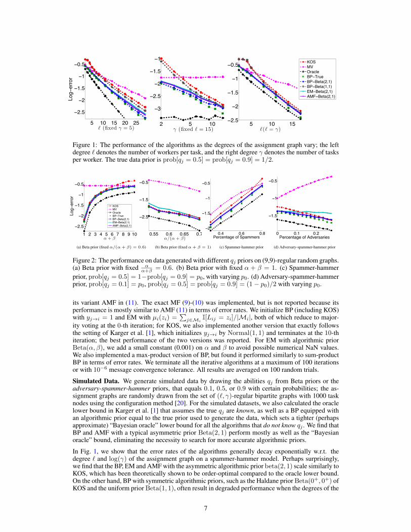
Figure 1: The performance of the algorithms as the degrees of the assignment graph vary; the leftdegree ` denotes the number of workers per task, and the right degree � denotes the number of tasksper worker. The true data prior is prob[q

j

= 0.5] = prob[qj

= 0.9] = 1/2.

1 2 3 4 5 6 7 8 9 10−2.5

−2

−1.5

−1

−0.5

α + β

Log−error

KOSMVOracleBP−TrueBP−Beta(2,1)EM−Beta(2,1)AMF−Beta(2,1)

0.55 0.6 0.65 0.7

−2.5

−1.5

−0.5

α/(α + β)0.4 0.6 0.8

−2

−1.5

−1

−0.5

Percentage of Spammers0 0.1 0.2

−1.5

−1

−0.5

Percentage of Adversaries

(a) Beta prior (fixed ↵/(↵ + �) = 0.6) (b) Beta prior (fixed ↵ + � = 1) (c) Spammer-hammer prior (d) Adversary-spammer-hammer prior

Figure 2: The performance on data generated with different qj

priors on (9,9)-regular random graphs.(a) Beta prior with fixed ↵

↵+�

= 0.6. (b) Beta prior with fixed ↵ + � = 1. (c) Spammer-hammerprior, prob[q

j

= 0.5] = 1�prob[qj

= 0.9] = p0, with varying p0. (d) Adversary-spammer-hammerprior, prob[q

j

= 0.1] = p0, prob[qj

= 0.5] = prob[qj

= 0.9] = (1� p0)/2 with varying p0.

its variant AMF in (11). The exact MF (9)-(10) was implemented, but is not reported because itsperformance is mostly similar to AMF (11) in terms of error rates. We initialize BP (including KOS)with y

j!i

= 1 and EM with µi

(zi

) =

Pj2Mi

I[Lij

= zi

]/|Mi

|, both of which reduce to major-ity voting at the 0-th iteration; for KOS, we also implemented another version that exactly followsthe setting of Karger et al. [1], which initializes y

j!i

by Normal(1, 1) and terminates at the 10-thiteration; the best performance of the two versions was reported. For EM with algorithmic priorBeta(↵,�), we add a small constant (0.001) on ↵ and � to avoid possible numerical NaN values.We also implemented a max-product version of BP, but found it performed similarly to sum-productBP in terms of error rates. We terminate all the iterative algorithms at a maximum of 100 iterationsor with 10

�6 message convergence tolerance. All results are averaged on 100 random trials.

Simulated Data. We generate simulated data by drawing the abilities qj

from Beta priors or theadversary-spammer-hammer priors, that equals 0.1, 0.5, or 0.9 with certain probabilities; the as-signment graphs are randomly drawn from the set of (`, �)-regular bipartite graphs with 1000 tasknodes using the configuration method [20]. For the simulated datasets, we also calculated the oraclelower bound in Karger et al. [1] that assumes the true q

j

are known, as well as a BP equipped withan algorithmic prior equal to the true prior used to generate the data, which sets a tighter (perhapsapproximate) “Bayesian oracle” lower bound for all the algorithms that do not know q

j

. We find thatBP and AMF with a typical asymmetric prior Beta(2, 1) perform mostly as well as the “Bayesianoracle” bound, eliminating the necessity to search for more accurate algorithmic priors.

In Fig. 1, we show that the error rates of the algorithms generally decay exponentially w.r.t. thedegree ` and log(�) of the assignment graph on a spammer-hammer model. Perhaps surprisingly,we find that the BP, EM and AMF with the asymmetric algorithmic prior beta(2, 1) scale similarly toKOS, which has been theoretically shown to be order-optimal compared to the oracle lower bound.On the other hand, BP with symmetric algorithmic priors, such as the Haldane prior Beta(0+, 0+) ofKOS and the uniform prior Beta(1, 1), often result in degraded performance when the degrees of the

7

5 10 15 200.1

0.2

0.3

0.4

0.5

Number of Workers per Task

Erro

r Rat

e

2 4 6 8 100.1

0.2

0.3

0.4

0.5

Number of Workers per Task2 4 6 8 10

0.1

0.2

0.3

0.4

Number of Workers per Task

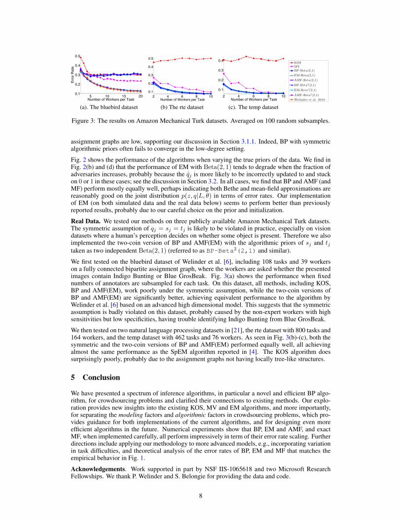
KOSMVBP-Beta(2,1)

EM-Beta(2,1)

AMF-Beta(2,1)

BP-Beta2(2,1)

EM-Beta2(2,1)

AMF-Beta2(2,1)

Welinder et al. 2010

(a). The bluebird dataset (b) The rte dataset (c). The temp dataset

Figure 3: The results on Amazon Mechanical Turk datasets. Averaged on 100 random subsamples.

assignment graphs are low, supporting our discussion in Section 3.1.1. Indeed, BP with symmetricalgorithmic priors often fails to converge in the low-degree setting.

Fig. 2 shows the performance of the algorithms when varying the true priors of the data. We find inFig. 2(b) and (d) that the performance of EM with Beta(2, 1) tends to degrade when the fraction ofadversaries increases, probably because the q

j

is more likely to be incorrectly updated to and stuckon 0 or 1 in these cases; see the discussion in Section 3.2. In all cases, we find that BP and AMF (andMF) perform mostly equally well, perhaps indicating both Bethe and mean-field approximations arereasonably good on the joint distribution p(z, q|L, ✓) in terms of error rates. Our implementationof EM (on both simulated data and the real data below) seems to perform better than previouslyreported results, probably due to our careful choice on the prior and initialization.

Real Data. We tested our methods on three publicly available Amazon Mechanical Turk datasets.The symmetric assumption of q

j

= sj

= tj

is likely to be violated in practice, especially on visiondatasets where a human’s perception decides on whether some object is present. Therefore we alsoimplemented the two-coin version of BP and AMF(EM) with the algorithmic priors of s

j

and tj

taken as two independent Beta(2, 1) (referred to as BP-Beta2(2,1) and similar).

We first tested on the bluebird dataset of Welinder et al. [6], including 108 tasks and 39 workerson a fully connected bipartite assignment graph, where the workers are asked whether the presentedimages contain Indigo Bunting or Blue GrosBeak. Fig. 3(a) shows the performance when fixednumbers of annotators are subsampled for each task. On this dataset, all methods, including KOS,BP and AMF(EM), work poorly under the symmetric assumption, while the two-coin versions ofBP and AMF(EM) are significantly better, achieving equivalent performance to the algorithm byWelinder et al. [6] based on an advanced high dimensional model. This suggests that the symmetricassumption is badly violated on this dataset, probably caused by the non-expert workers with highsensitivities but low specificities, having trouble identifying Indigo Bunting from Blue GrosBeak.

We then tested on two natural language processing datasets in [21], the rte dataset with 800 tasks and164 workers, and the temp dataset with 462 tasks and 76 workers. As seen in Fig. 3(b)-(c), both thesymmetric and the two-coin versions of BP and AMF(EM) performed equally well, all achievingalmost the same performance as the SpEM algorithm reported in [4]. The KOS algorithm doessurprisingly poorly, probably due to the assignment graphs not having locally tree-like structures.

5 Conclusion

We have presented a spectrum of inference algorithms, in particular a novel and efficient BP algo-rithm, for crowdsourcing problems and clarified their connections to existing methods. Our explo-ration provides new insights into the existing KOS, MV and EM algorithms, and more importantly,for separating the modeling factors and algorithmic factors in crowdsourcing problems, which pro-vides guidance for both implementations of the current algorithms, and for designing even moreefficient algorithms in the future. Numerical experiments show that BP, EM and AMF, and exactMF, when implemented carefully, all perform impressively in term of their error rate scaling. Furtherdirections include applying our methodology to more advanced models, e.g., incorporating variationin task difficulties, and theoretical analysis of the error rates of BP, EM and MF that matches theempirical behavior in Fig. 1.

Acknowledgements. Work supported in part by NSF IIS-1065618 and two Microsoft ResearchFellowships. We thank P. Welinder and S. Belongie for providing the data and code.

8

References[1] D.R. Karger, S. Oh, and D. Shah. Iterative learning for reliable crowdsourcing systems. In

Neural Information Processing Systems (NIPS), 2011.[2] A.P. Dawid and A.M. Skene. Maximum likelihood estimation of observer error-rates using the

em algorithm. Applied Statistics, pages 20–28, 1979.[3] P. Smyth, U. Fayyad, M. Burl, P. Perona, and P. Baldi. Inferring ground truth from subjective

labelling of venus images. Advances in neural information processing systems, pages 1085–1092, 1995.

[4] V.C. Raykar, S. Yu, L.H. Zhao, G.H. Valadez, C. Florin, L. Bogoni, and L. Moy. Learningfrom crowds. The Journal of Machine Learning Research, 11:1297–1322, 2010.

[5] J Whitehill, P Ruvolo, T Wu, J Bergsma, and J Movellan. Whose vote should count more:Optimal integration of labels from labelers of unknown expertise. In Advances in NeuralInformation Processing Systems, pages 2035–2043. 2009.

[6] P. Welinder, S. Branson, S. Belongie, and P. Perona. The multidimensional wisdom of crowds.In Neural Information Processing Systems Conference (NIPS), 2010.

[7] V.C. Raykar and S. Yu. Eliminating spammers and ranking annotators for crowdsourced label-ing tasks. Journal of Machine Learning Research, 13:491–518, 2012.

[8] Fabian L. Wauthier and Michael I. Jordan. Bayesian bias mitigation for crowdsourcing. InAdvances in Neural Information Processing Systems 24, pages 1800–1808. 2011.

[9] B. Carpenter. Multilevel bayesian models of categorical data annotation. Unpublishedmanuscript, 2008.

[10] D. Koller and N. Friedman. Probabilistic graphical models: principles and techniques. MITpress, 2009.

[11] M. Wainwright and M. Jordan. Graphical models, exponential families, and variational infer-ence. Found. Trends Mach. Learn., 1(1-2):1–305, 2008.

[12] Y. Weiss and W.T. Freeman. On the optimality of solutions of the max-product belief-propagation algorithm in arbitrary graphs. Information Theory, IEEE Transactions on, 47(2):736 –744, Feb 2001.

[13] F.R. Kschischang, B.J. Frey, and H.A. Loeliger. Factor graphs and the sum-product algorithm.Information Theory, IEEE Transactions on, 47(2):498–519, 2001.

[14] D. Tarlow, I.E. Givoni, and R.S. Zemel. Hopmap: Efficient message passing with high orderpotentials. In Proc. of AISTATS, 2010.

[15] A. Zellner. An introduction to Bayesian inference in econometrics, volume 17. John Wiley andsons, 1971.

[16] R.E. Kass and L. Wasserman. The selection of prior distributions by formal rules. Journal ofthe American Statistical Association, pages 1343–1370, 1996.

[17] F. Tuyl, R. Gerlach, and K. Mengersen. A comparison of bayes-laplace, jeffreys, and otherpriors. The American Statistician, 62(1):40–44, 2008.

[18] Radford Neal and Geoffrey E. Hinton. A view of the EM algorithm that justifies incremental,sparse, and other variants. In M. Jordan, editor, Learning in Graphical Models, pages 355–368.Kluwer, 1998.

[19] A. Asuncion. Approximate mean field for Dirichlet-based models. In ICML Workshop onTopic Models, 2010.

[20] B. Bollobas. Random graphs, volume 73. Cambridge Univ Pr, 2001.[21] R. Snow, B. O’Connor, D. Jurafsky, and A.Y. Ng. Cheap and fast—but is it good?: evaluating

non-expert annotations for natural language tasks. In Proceedings of the Conference on Empir-ical Methods in Natural Language Processing, pages 254–263. Association for ComputationalLinguistics, 2008.

9

000001002003004005006007008009010011012013014015016017018019020021022023024025026027028029030031032033034035036037038039040041042043044045046047048049050051052053

This document contains derivations and other supplemental information for the NIPS 2012 submis-sion, “Variational Inference for Crowdsourcing”.

A Derivation of the Belief Propagation Algorithm

A.1 Sum-product Belief Propagation

We derive the belief propagation algorithm (15) in Theorem 3.1.

Theorem 3.1.

Let xi

= log

bi

(+1)

bi

(�1)

, xi!j

= log

mi!j

(+1)

mi!j

(�1)

, and yj!i

= Lij

log

mj!i

(+1)

mi!j

(�1)

.

Then, sum-product BP (5)-(7) can be expressed as

xt+1i!j

=

X

j

02Mi\j

Lij

ytj

0!i

, yt+1j!i

= log

P�j�1k=0 (k + 1, �

j

)et+1kP

�j�1k=0 (k, �

j

)et+1k

, (1)

and xt+1i

=

Pj2Mi

Lij

yt+1i!j

, where the terms ek

for k = 0, . . . , Nj

� 1, are the

elementary symmetric polynomials in variables {exp(Li

0j

xi

0!j

)}i

02Nj\i , that is, ek

=Ps : |s|=k

Qi

02s

exp(Li

0j

xi

0!j

). In the end, the true labels are decoded as zti

= sign[xt

i

].

Proof. First, by update (5), we have

xt+1i!j

= log

mt

j!i

(+1)

mt

j!i

(�1)

= log

Qj

0!Mi\jmt

j!i

(+1)

Qj

0!Mi\jmt

j!i

(�1)

=

X

j

02Mi\j

Lij

yti!j

0 .

Similar derivation applies to update (7). We just need to consider the update (6) in the following.

For a given z, we define N+j\i[z] = {i0 2 N

j\i : zi0 = Li

0j

}. Let Ak

:

= {zNj\i : |N+j\i[z]| = k}. By

update (6) we have,

mt+1j!i

(+Lij

) =

X

zNj\i

j

(zNj )

Y

i

02Nj\i

mt+1i

0!j

(z0i

) (2)

=

�j�1X

k=0

j

(k + 1, �j

)

X

z2Ak

Y

i

02Nj\i

mt+1i

0!j

(z0i

) (3)

= C

�j�1X

k=0

j

(k + 1, �j

)

X

z2Ak

Y

i

02Nj\i

mt+1i

0!j

(z0i

)

mt+1i

0!j

(�Li

0j

)

(4)

= C

�j�1X

k=0

j

(k + 1, �j

)

X

z2Ak

Y

i

02N+j\i[z]

mt+1i

0!j

(Li

0j

)

mt+1i

0!j

(�Li

0j

)

(5)

= C

�j�1X

k=0

j

(k + 1, �j

)

X

z2Ak

Y

i

02N+j\i[z]

exp(xt+1i

0!j

) (6)

= C

�j�1X

k=0

j

(k + 1, �j

)ek

, (7)

where C is a constant, C = (

Qi

02Nj\imt+1

i

0!j

(�Li

0j

)). Similarily, one can show that

mt+1j!i

(�Lij

) = C

�j�1X

k=0

j

(k, �j

)ek

. (8)

1

054055056057058059060061062063064065066067068069070071072073074075076077078079080081082083084085086087088089090091092093094095096097098099100101102103104105106107

Therefore, we have

yt+1j!i

= log

mt+1j!i

(+Lij

)

mt+1j!i

(�Lij

)

= log

P�j�1k=0

j

(k + 1, �j

)ekP

�j�1k=0

j

(k, �j

)ek

.

The proof is completed.

It remains a problem to calculate the elementary symmetric polynomials ek

. Here we present adivide and conquer algorithm with a running time of O(�

j

(log �j

)

2). Note that e

k

is the k-th coef-ficient of polynomial

Q�j�1i=0 (x + exi

), where exi= exp(x

i!j

). We divide the polynomial into aproduct of two polynomials,

�j�1Y

i=0

(x+ exi) =

� d �j2 eY

i=0

(x+ exi)

·� �j�1Y

i=d �j2 e

(x+ exi)

.

Since the merging step requires a polynomial multiplication, which is solved by fast Fourier trans-formation with O(�

j

log �j

), by the master theorem, we get a total cost of O(�j

(log �j

)

2).

A more straightforward algorithm can be derived via dynamic programming, but with a higher costof O(�2

j

). Let e(k, n) be the k-th symmetric polynomial of the first n numbers of {xe

i

}i

02Nj\i ; onecan calculate e

k

through the recursive formula e(k, n) = e(k, n� 1)exn+ e(k, n).

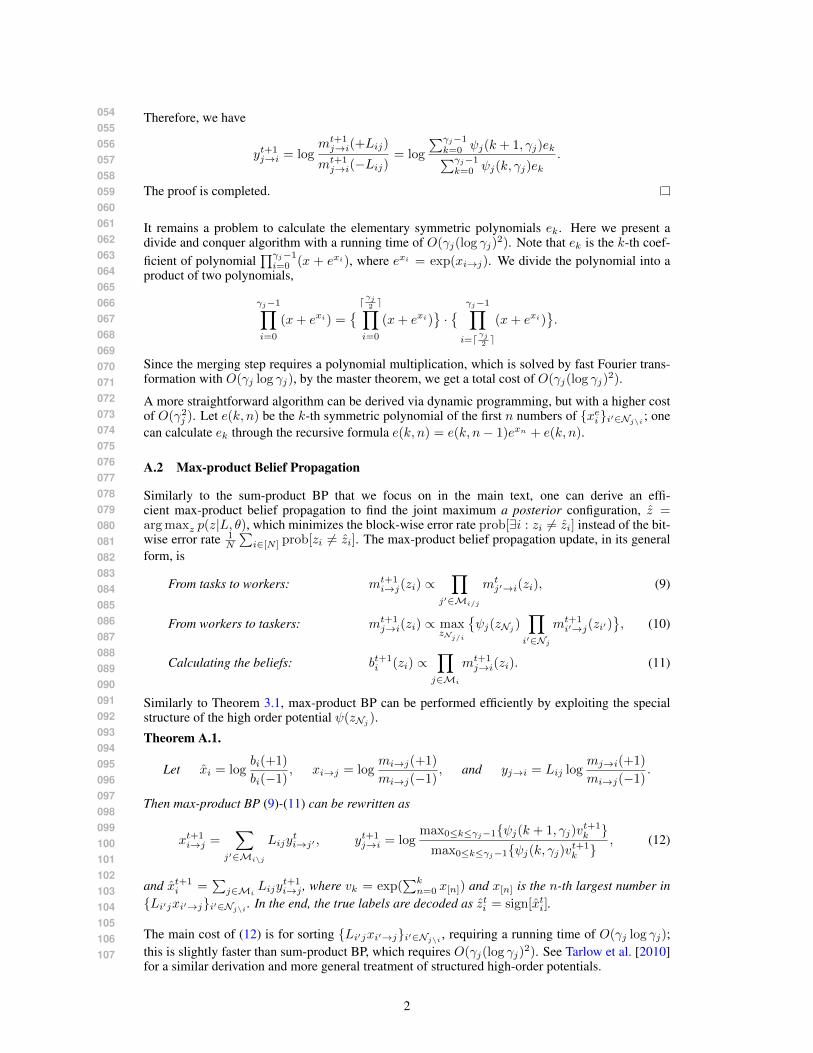
A.2 Max-product Belief Propagation

Similarly to the sum-product BP that we focus on in the main text, one can derive an effi-cient max-product belief propagation to find the joint maximum a posterior configuration, z =

argmax

z

p(z|L, ✓), which minimizes the block-wise error rate prob[9i : zi

6= zi

] instead of the bit-wise error rate 1

N

Pi2[N ] prob[zi 6= z

i

]. The max-product belief propagation update, in its generalform, is

From tasks to workers: mt+1i!j

(zi

) /Y

j

02Mi/j

mt

j

0!i

(zi

), (9)

From workers to taskers: mt+1j!i

(zi

) / max

zNj/i

� j

(zNj )

Y

i

02Nj

mt+1i

0!j

(zi

0)

, (10)

Calculating the beliefs: bt+1i

(zi

) /Y

j2Mi

mt+1j!i

(zi

). (11)

Similarly to Theorem 3.1, max-product BP can be performed efficiently by exploiting the specialstructure of the high order potential (zNj ).Theorem A.1.

Let xi

= log

bi

(+1)

bi

(�1)

, xi!j

= log

mi!j

(+1)

mi!j

(�1)

, and yj!i

= Lij

log

mj!i

(+1)

mi!j

(�1)

.

Then max-product BP (9)-(11) can be rewritten as

xt+1i!j

=

X

j

02Mi\j

Lij

yti!j

0 , yt+1j!i

= log

max0k�j�1{ j

(k + 1, �j

)vt+1k

}max0k�j�1{ j

(k, �j

)vt+1k

}, (12)

and xt+1i

=

Pj2Mi

Lij

yt+1i!j

, where vk

= exp(

Pk

n=0 x[n]) and x[n] is the n-th largest number in

{Li

0j

xi

0!j

}i

02Nj\i . In the end, the true labels are decoded as zti

= sign[xt

i

].

The main cost of (12) is for sorting {Li

0j

xi

0!j

}i

02Nj\i , requiring a running time of O(�j

log �j

);this is slightly faster than sum-product BP, which requires O(�

j

(log �j

)

2). See Tarlow et al. [2010]

for a similar derivation and more general treatment of structured high-order potentials.

2

108109110111112113114115116117118119120121122123124125126127128129130131132133134135136137138139140141142143144145146147148149150151152153154155156157158159160161

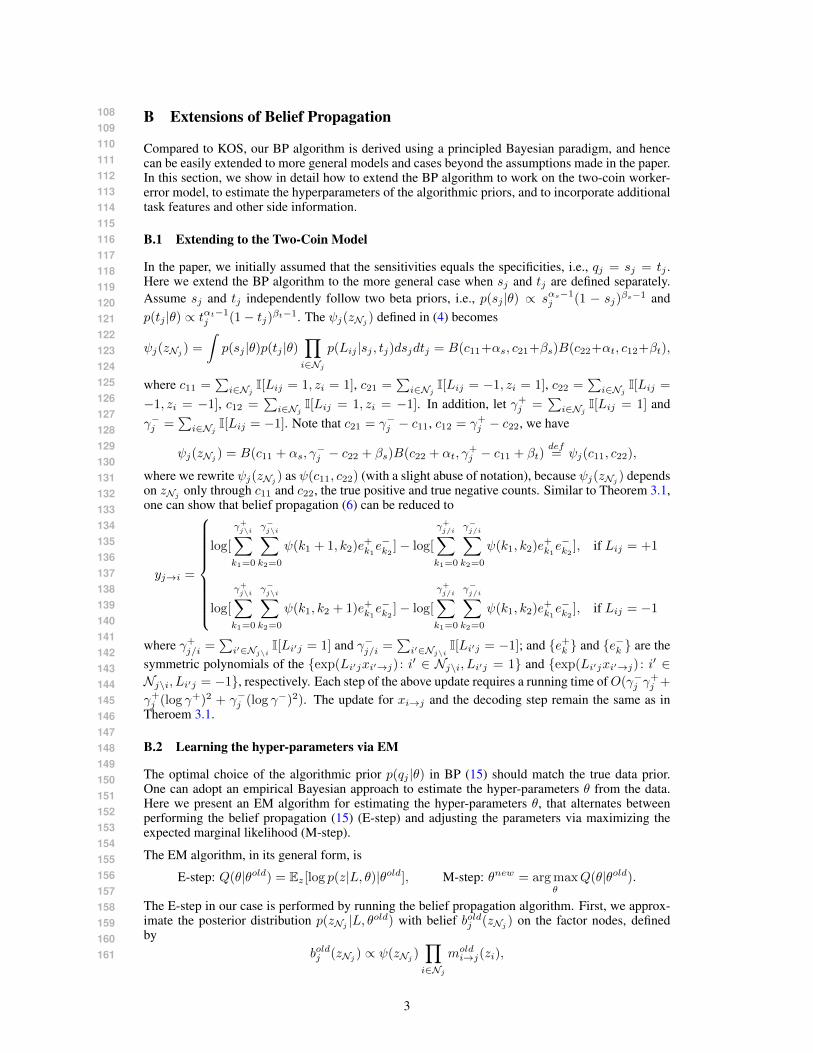
B Extensions of Belief Propagation

Compared to KOS, our BP algorithm is derived using a principled Bayesian paradigm, and hencecan be easily extended to more general models and cases beyond the assumptions made in the paper.In this section, we show in detail how to extend the BP algorithm to work on the two-coin worker-error model, to estimate the hyperparameters of the algorithmic priors, and to incorporate additionaltask features and other side information.

B.1 Extending to the Two-Coin Model

In the paper, we initially assumed that the sensitivities equals the specificities, i.e., qj

= sj

= tj

.Here we extend the BP algorithm to the more general case when s

j

and tj

are defined separately.Assume s

j

and tj

independently follow two beta priors, i.e., p(sj

|✓) / s↵s�1j

(1 � sj

)

�s�1 andp(t

j

|✓) / t↵t�1j

(1� tj

)

�t�1. The j

(zNj ) defined in (4) becomes

j

(zNj ) =

Zp(s

j

|✓)p(tj

|✓)Y

i2Nj

p(Lij

|sj

, tj

)dsj

dtj

= B(c11+↵s

, c21+�s)B(c22+↵t

, c12+�t),

where c11 =

Pi2Nj

I[Lij

= 1, zi

= 1], c21 =

Pi2Nj

I[Lij

= �1, zi

= 1], c22 =

Pi2Nj

I[Lij

=

�1, zi

= �1], c12 =

Pi2Nj

I[Lij

= 1, zi

= �1]. In addition, let �+j

=

Pi2Nj

I[Lij

= 1] and��j

=

Pi2Nj

I[Lij

= �1]. Note that c21 = ��j

� c11, c12 = �+j

� c22, we have

j

(zNj ) = B(c11 + ↵s

, ��j

� c22 + �s

)B(c22 + ↵t

, �+j

� c11 + �t

)

def

= j

(c11, c22),

where we rewrite j

(zNj ) as (c11, c22) (with a slight abuse of notation), because j

(zNj ) dependson zNj only through c11 and c22, the true positive and true negative counts. Similar to Theorem 3.1,one can show that belief propagation (6) can be reduced to

yj!i

=

8>>>>>>>><

>>>>>>>>:

log[

�

+j\iX

k1=0

�

�j\iX

k2=0

(k1 + 1, k2)e+k1e�k2]� log[

�

+j/iX

k1=0

�

�j/iX

k2=0

(k1, k2)e+k1e�k2], if L

ij

= +1

log[

�

+j\iX

k1=0

�

�j\iX

k2=0

(k1, k2 + 1)e+k1e�k2]� log[

�

+j/iX

k1=0

�

�j/iX

k2=0

(k1, k2)e+k1e�k2], if L

ij

= �1

where �+j/i

=

Pi

02Nj\iI[L

i

0j

= 1] and ��j/i

=

Pi

02Nj\iI[L

i

0j

= �1]; and {e+k

} and {e�k

} are thesymmetric polynomials of the {exp(L

i

0j

xi

0!j

) : i0 2 Nj\i, Li

0j

= 1} and {exp(Li

0j

xi

0!j

) : i0 2N

j\i, Li

0j

= �1}, respectively. Each step of the above update requires a running time of O(��j

�+j

+

�+j

(log �+)2 + ��j

(log ��)2). The update for xi!j

and the decoding step remain the same as inTheroem 3.1.

B.2 Learning the hyper-parameters via EM

The optimal choice of the algorithmic prior p(qj

|✓) in BP (15) should match the true data prior.One can adopt an empirical Bayesian approach to estimate the hyper-parameters ✓ from the data.Here we present an EM algorithm for estimating the hyper-parameters ✓, that alternates betweenperforming the belief propagation (15) (E-step) and adjusting the parameters via maximizing theexpected marginal likelihood (M-step).

The EM algorithm, in its general form, is

E-step: Q(✓|✓old) = Ez

[log p(z|L, ✓)|✓old], M-step: ✓new = argmax

✓

Q(✓|✓old).

The E-step in our case is performed by running the belief propagation algorithm. First, we approx-imate the posterior distribution p(zNj |L, ✓old) with belief bold

j

(zNj ) on the factor nodes, definedby

boldj

(zNj ) / (zNj )

Y

i2Nj

mold

i!j

(zi

),

3

162163164165166167168169170171172173174175176177178179180181182183184185186187188189190191192193194195196197198199200201202203204205206207208209210211212213214215

where mold

i!j

are the messages of belief propagation when ✓ = ✓old. The E-step becomes

Q(✓|✓t) = Ez

[log p(z|L, ✓)|✓t] =X

j

X

zNj

boldj

(zNj ) log j

(zNj |L, ✓). (13)

Similar to Theorem 3.1, one can calculate (13) in terms of the elementary symmetric polynomialsek

; one can show that

Q(✓|✓t) =X

j

�jX

k=0

yoldk

log j

(k, �j

|L, ✓), (14)

where yoldk

= j

(k, �j

|L, ✓old)eoldk

, where eoldk

are the elementary symmetric polynomials of{exp(L

ij

xold

i!j

) : i 2 Nj

}.

The M-step in our case can be efficiently solved using standard numerical methods. For example,when the algorithmic priors of q

j

is Beta(↵,�) where ✓ = [↵,�], one can show that Q(✓|✓old)equals (up to a constant) the log-likelihood of Beta-binomial distribution, and can be efficientlymaximized using standard numerical methods.

The E-step above takes a soft combination of the posterior evidence. An alternative is to use hard-EM, which replaces the E-step with

E-step (hard-EM): Q(✓|✓old) = log p(zold|L, ✓),where zold are the estimated labels via belief propagation on ✓ = ✓old. The hard-EM form is veryintuitive; it iteratively estimates the labels with belief propagation, and fits the hyper-parametersimputed with the labels found by the last estimation.

Note that this form of EM (in the outer loop) for estimating the hyper-parameters is different fromEM (in the inner loop) of Dawid and Skene [1979], Smyth et al. [1995], Raykar et al. [2010], whichmaximizes q

j

with fixed hyper-parameter ✓; it is closer to the SpEM of Raykar and Yu [2012],which also estimates a hyper-parameter with q

j

marginalized, but uses a different EM and Laplacianapproximation in the inner loop.

B.3 Incorporating Task Features

In some cases the tasks are associated with known features that provide additional information aboutthe true labels, and the problem is formulated as a supervised learning task with crowdsourced(redundant but noisy) labels [Raykar et al., 2010]. Our method can be easily extended to these casesby representing the task features as singleton potentials on the variables nodes in the factor graph,that is, the posterior distribution (4) is modified to

p(z|F,L, ✓,!) =Y

i

p(zi

|fi

;!)Y

j

(zNj ),

where F = {fj

: j 2 [N ]} are the features of the tasks, and ! are the regression coefficients. Ourbelief propagation works here with only minor modification. The regression coefficient !, togetherwith the hyper-parameter ✓, can be estimated using the EM algorithm we discussed above.

B.4 Incorporating Partially Known Ground Truth

In case the ground truth labels of some tasks are known, these labels can help the prediction of theother tasks via a “wave effect”, propagating information about the reliabilities of their associatedworkers. Our algorithm can also be easily extended to this case.

Specifically, assume the ground truth labels of a subset of tasks G 2 [N ] are known, e.g., zG

= z0G

.Let ↵

j

be the number of tasks in G that worker j labels correctly. To predict the remaining labels,one can simply modify the BP algorithm (15) into

xt+1i!j

=

X

j

02Mi\j

Lij

yti!j

0 , yj!i

= log

P�j�1k=0

j

(k + ↵j

+ 1, �j

)ekP

�j�1k=0

j

(k + ↵j

, �j

)ek

, (15)

where the messages are passed only between the workers and the tasks with unknown labels. In-tuitively, the known ground truth provides scores (in term of ↵

j

) of the workers who have labeledthem, which are used as “prior” information for predicting the remaining labels.

4