
0 Lecture Nine FINA 522: Project Finance and Risk Management Updated: 29 April, 2007.
99
1 Lecture Nine FINA 522: Project Finance and Risk Management Updated: 29 April, 2007
-
Upload
isabel-peters -
Category
Documents
-
view
215 -
download
0
Transcript of 0 Lecture Nine FINA 522: Project Finance and Risk Management Updated: 29 April, 2007.

1
Lecture Nine
FINA 522: Project Finance and Risk Management
Updated: 29 April, 2007

RISK ANALYSIS
3
What is risk?
• Risk generally describes the possible deviation from a projected outcome.
• To project any uncertain outcome into the future you need to have a “predictive model”.
• A predictive model could be a simple formula or a very complex worksheet.

4
Decision-Making Under Uncertainty
1.Risk analysis• How to identify, analyze, and interpret the
expected variability in project outcomes
2.Risk diversification and management• How to diversify unsystematic risk• How to redesign and reorganize projects in
order to reallocate risk

5
Risk Analysis1. WHY?
• Project returns are spread over time
• Each variable affecting NPV is subject to a high level
of uncertainty
• Information and data needed for more accurate
forecasts are costly to acquire
• Need to reduce the likelihood of undertaking a "bad"
project while not failing to accept a "good" project

6
A good predictive model in project appraisal depends on:
Cash-Flow Projections Marketing Module
Technical Module
Input Data
Input Data
Correct methodology Accurate data
7
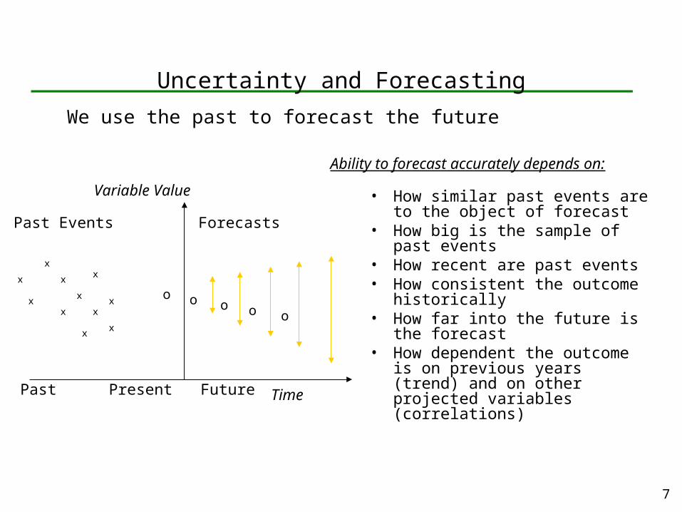
Uncertainty and Forecasting
• How similar past events are to the object of forecast
• How big is the sample of past events• How recent are past events• How consistent the outcome
historically• How far into the future is the forecast• How dependent the outcome is on
previous years (trend) and on other projected variables (correlations)
x
x
x
x
xx
x
x
xx
x
o o o o o
TimePresentPast Future
Variable Value
Past Events Forecasts
We use the past to forecast the future
Ability to forecast accurately depends on:

8
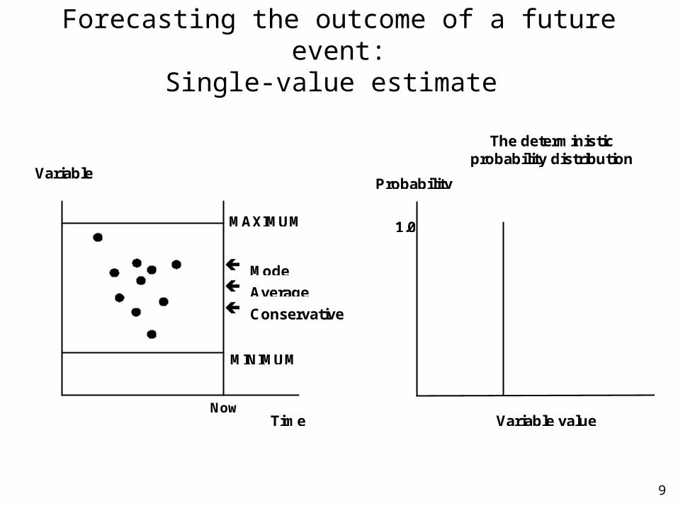
Inputs are projected as certainties(Base Case Scenario)
• When we provide inputs to a predictive model we use one particular probability distribution – the Deterministic Probability Distribution.
• By that we assign 100% probability that the single value of the input we use in the projection will actually arise.
9
MAXIMUM 1.0
Mode Average Conservative
estimateMINIMUM
Now
The deterministicprobability distribution
Probability Variable
value
Time Variable value
Forecasting the outcome of a future event:Single-value estimate
10
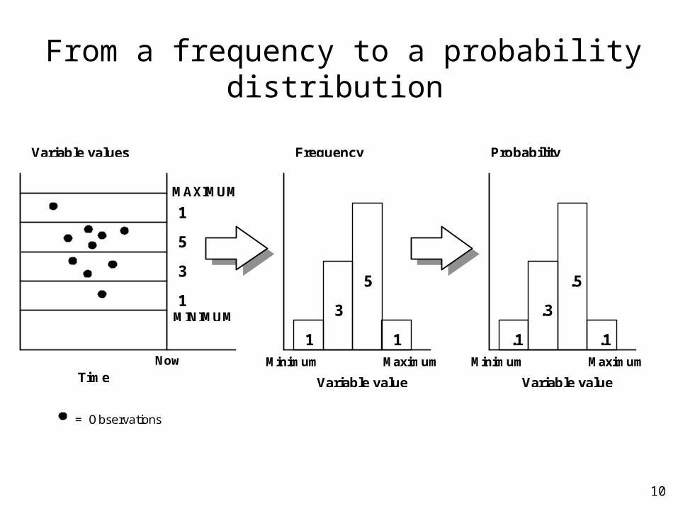
From a frequency to a probability distribution
MAXIMUM
1
5
53
31
11
MINIMUM
MaximumNow Minimum
ProbabilityFrequencyVariable values
Time Variable value
.5
.3
.1.1MaximumMinimum
Variable value
= Observations
11
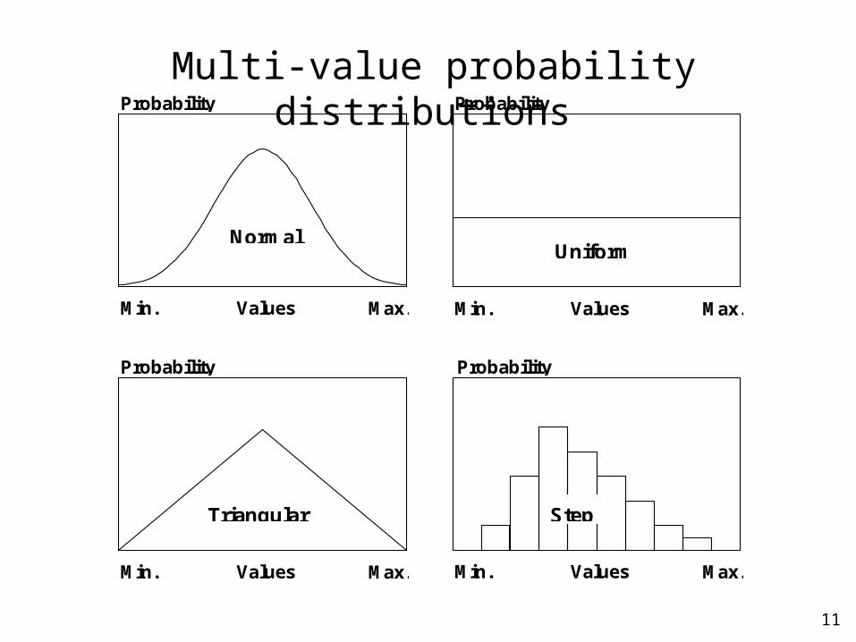
Multi-value probability distributions
Normal
Probability
Values Max.Min.
Probability
Uniform
Values Max.Min.
Probability
Triangular
Values Max.Min.
Probability
Step
Values Max.Min.

12
Multi-value probability distributions as their inputs to a predictive model.
• Any possible deviation in any of the critical input variables of a predictive model from their base case values will generate a new scenario with a different outcome (or outcomes).
• There are potentially an infinite number of combinations of input values possible, each causing a different set of results.
13
2. Alternative Methods of Dealing With Risk
2.1 Sensitivity Analysis
2.2 Scenario Analysis
2.3 Monte Carlo Risk Analysis(or Simulation Analysis)
14
2.1 Sensitivity Analysis• Test the sensitivity of a project's outcome (NPV or the key
variable) to changes in value of one parameter at a time• "What if" analysis• Allows you to test which variables are important as a source
of risk • A variable is important depending on:
A) Its share of total benefits or costs
B) Likely range of values• Sensitivity analysis allows you to determine the direction of
change in the NPV• Break-even analysis allows you to determine how much a
variable must change before the NPV or these key variable moves into its critical range turns negative
15
Another Important Use of Sensitivity Analysis
• Sensitivity analysis on the PV of each row of the spreadsheet (Banker’s, Owner’s and Economy’s point of view) is the best way to de-bug a spreadsheet
• If results do not make sense then it is likely that there is an computation or logistical error in the spreadsheet
16
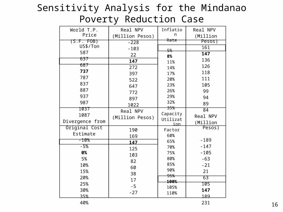
Sensitivity Analysis for the Mindanao Poverty Reduction Case
Inflation Rate5%8%11%14%17%20%23%26%29%32%35%
CapacityUtilization
Factor60%65%70%75%80%85%90%95%100%105%110%
Real NPV (Million Pesos)
16114713612611811110599948984
Real NPV(Million Pesos)
-189-147-105-63-212163
105147189231
World T.P. Price(S.F. FOB) US$/Ton
587637687737787837887937987
10371087
Divergence fromOriginal Cost
Estimate-10%-5%0%5%
10%15%20%25%30%35%40%
Real NPV (Million Pesos)
-228-10322
147272397522647772897
1022Real NPV
(Million Pesos)
19016914712510382603817-5
-27
17
• For Tomato Paste Plant Capacity Utilization is critical.
• What can cause Capacity Utilization to be low?1. Technical problems with the plant.
2. The demand for product does not exist at the price that covers the costs
3. The plant can not get adequate supplies of raw materials.
Factsheet: – this plant eventually run into financial troubles– could not attain adequate supplies of raw
materials

18
Cautionary Notes for Sensitivity Analysis1. Range and probability distribution of variables
• Sensitivity analysis doesn't represent the possible range
of values
• Sensitivity analysis doesn't represent the probabilities for
each range. Generally there is a small probability of being
at the extremes.
2. Direction of effectsFor most variables, the direction is obvious
A) Revenue increases NPV increasesB) Cost increases NPV decreasesC) Inflation Not so obvious

19
Cautionary Notes for Sensitivity Analysis 3. One-at-a-Time Testing Is Not Realistic
• One-at-a-time testing is not realistic because of correlation
among variables
A) If Q sold increases, costs will increase
Profits = Q (P - UC)
B) If inflation rate changes, all prices change
C) If exchange rate changes, all tradable goods' prices and foreign
liabilities change
• One method of dealing with these combined or correlated
effects is scenario analysis
20
2.2 Scenario Analysis• Scenario analysis recognizes that certain variables are interrelated. Thus a small number of
variables can be altered in a consistent manner at the same time.
• What is the set of circumstances that are likely to combine to produce different "cases" or "scenarios"?
A. Worst case / Pessimistic case
B. Expected case / Best estimate case
C. Best case / Optimistic caseNote: Scenario analysis does not take into account the Probability of cases arising
• Interpretation is easy when results are robust:
A. Accept project if NPV > 0 even in the worst case
B. Reject project if NPV < 0 even in the best case
C. If NPV is positive in some cases and negative in other cases, then results are not conclusive
• Difficult to define what scenario’s to specify without first examining the range of possible outcomes by a Monte Carlo Analysis.
• Scenario analysis is a good way to communicate the results of a Monte Carlo analysis.

21
2.3 Monte Carlo Method of Risk Analysis
• A natural extension of sensitivity and scenario analysis
• Simultaneously takes into account different probability distributions and different ranges of possible values for key project variables
• Allows for correlation (covariation) between variables
• Generates a probability distribution of project outcomes (NPV) instead of just a single value estimate
• The probability distribution of project outcomes may assist decision-makers in making choices, but there can be problems of interpretation and use.
22
Monte-Carlo Simulation
• Monte Carlo simulation is a methodology that handles the complexity arising from projecting multi-value probability distributions as inputs to a model.
• Practically this is only possible to be applied with the use of a computer and specialised software.

23
The Risk Analysis Process
Probability distri-butions (step 1)
Definition of range limits for possible variable values
Risk variables
Selection of key project variables
Forecasting model
Preparation of a model capable of predicting reality
Probability distri-butions (step 2)
Allocation of probability weights to range of values
Simulation runs
Generation of random scenarios based on assumptions set
Correlation conditions
Setting of relationships for correlated variables
Analysis of results
Statistical analysis of the output of simulation

24
Simple Model
B-C
Relationships ResultVariables
B=3
C=2R=1
25
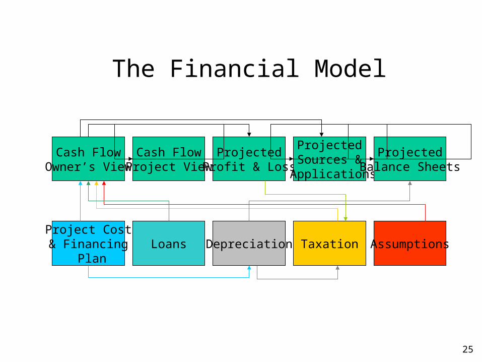
The Financial Model
Cash FlowOwner’s View
Cash FlowProject View
ProjectedProfit & Loss
ProjectedSources &
Applications
ProjectedBalance Sheets
Loans Depreciation TaxationProject Cost& Financing
PlanAssumptions
26
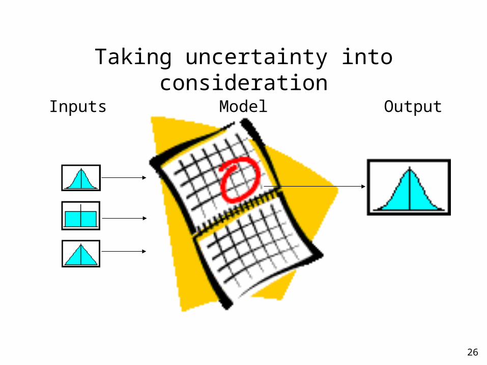
Taking uncertainty into consideration
Inputs OutputModel
27
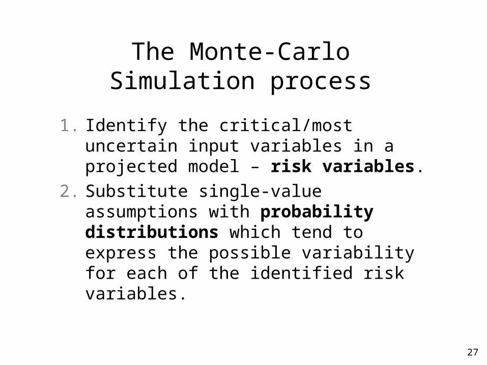
The Monte-Carlo Simulation process
1. Identify the critical/most uncertain input variables in a projected model – risk variables.
2. Substitute single-value assumptions with probability distributions which tend to express the possible variability for each of the identified risk variables.

28
Forecasting Model
Forecasting Model
$ Variables Formulae
Sales price 12 V1
Volume of sales 100 V2
Cash inflow 1,200 F1 = V1 V2
Materials 300 F2 = V2 V4
Wages 400 F3 = V2 V5
Expenses 200 V3
Cash outflow 900 F4 = F2 + F3 + V3
Net Cash Flow 300 F5 = F1 – F4
Relevant assumptions
Material cost per unit 3.00 V4
Wages per unit 4.00 V5

29
Set Probability Distributions Simulation model
$ Risk variables
Sales price 12 V1
Volume of sales 100 V2
Cash inflow 1,200
Materials 300
Wages 400
Expenses 200
Cash outflow 900
Net Cash Flow 300
Relevant assumptions
Material cost per unit 3.00 V4
Wages per unit 4.00
X
-0.8
Y
30
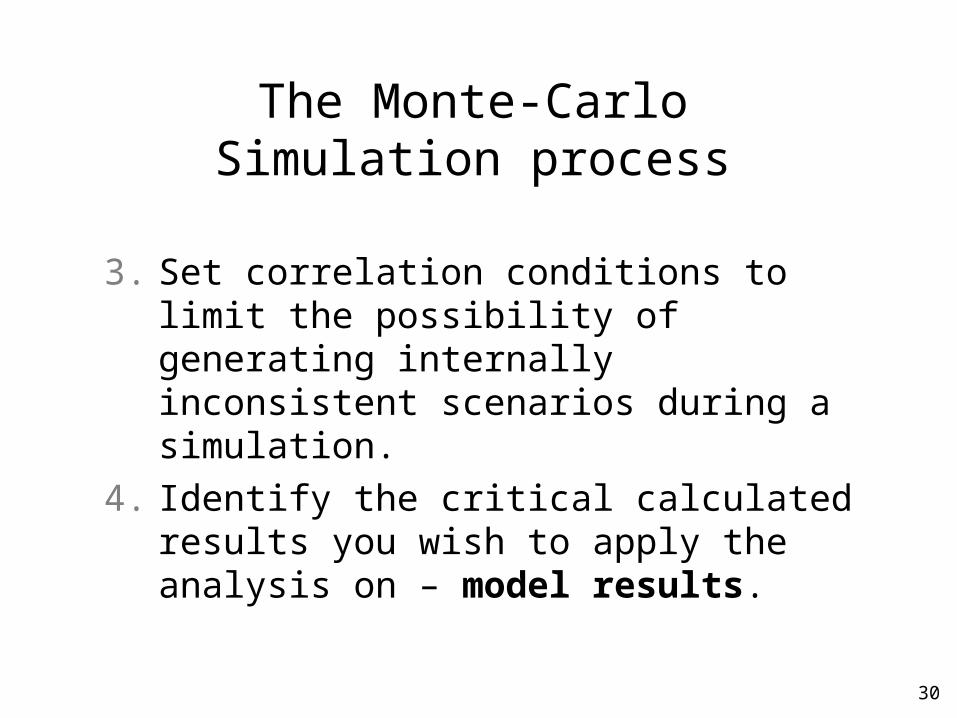
The Monte-Carlo Simulation process
3. Set correlation conditions to limit the possibility of generating internally inconsistent scenarios during a simulation.
4. Identify the critical calculated results you wish to apply the analysis on – model results.

31
Set correlation conditionsSimulation model
$ Risk variables
Sales price 12 V1
Volume of sales 100 V2
Cash inflow 1,200
Materials 300
Wages 400
Expenses 200
Cash outflow 900
Net Cash Flow 300
Relevant assumptions
Material cost per unit 3.00 V4
Wages per unit 4.00
X
-0.8
Y

32
Correlated variables – Generating Relationship Data
Correlated Variables(r = 0.8), 200 runs
8 9 10 11 12 13 14 15 16
Sales price (independent variable)
70
80
90
100
110
120
130
Vo
lum
e o
f sa
les
(dep
end
ent
vari
able
)

33
5. Run simulation creating a sample of computer scenarios based on inputs from the probability distributions and with respect to any correlation conditions set.
6. Analyse results generated in the simulation run, calculating statistical measures and plotting probability distribution graphs of the results, which indicate all the potential outcomes and their likelihood of occurrence.
The Monte-Carlo Simulation process

34
Simulation Runs
35
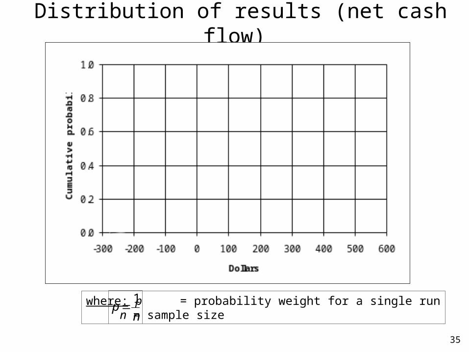
Distribution of results (net cash flow)
pn
1 where: p = probability weight for a single run
n = sample size

36
Net present value distribution (different project perspectives)
0.00
0.20
0.40
0.60
0.80
1.00
-300000 -200000 -100000 0 100000 200000 300000
Banker's view Ow ner's view Economy's view
Cumulative probability

37
Time
Mastering Cash Flow - What lies beneath the projections?CashFlow
Base-Case Cash flow
38
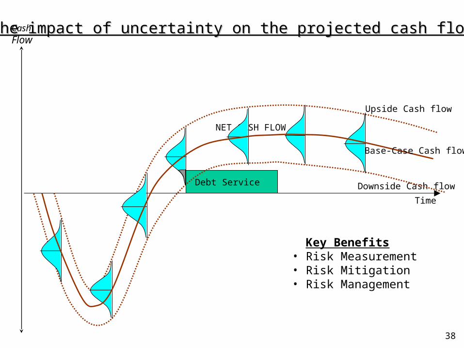
Time
The impact of uncertainty on the projected cash flowThe impact of uncertainty on the projected cash flow
Debt Service
CashFlow
Downside Cash flow
Upside Cash flow
NET CASH FLOW
Base-Case Cash flow
Key Benefits • Risk Measurement• Risk Mitigation• Risk Management
39
Interpretation of Risk Analysis Results
40

41
Case 1: Probability of negative NPV=0
+- 0NPV
+- 0NPV
ProbabilityCumulative probability
DECISION : ACCEPT

42
Case 2: Probability of positive NPV=0
+- 0NPV
+- 0NPV
ProbabilityCumulative probability
DECISION : REJECT
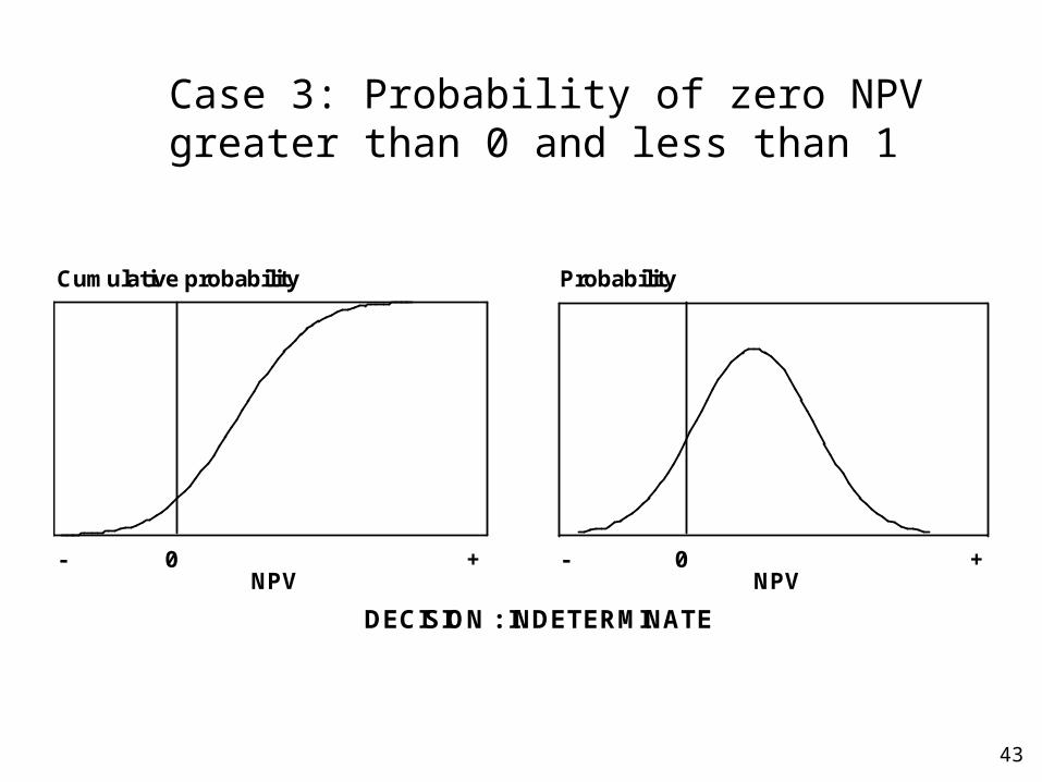
43
Case 3: Probability of zero NPV greater than 0 and less than 1
+- 0NPV
+- 0NPV
ProbabilityCumulative probability
DECISION : INDETERMINATE
44
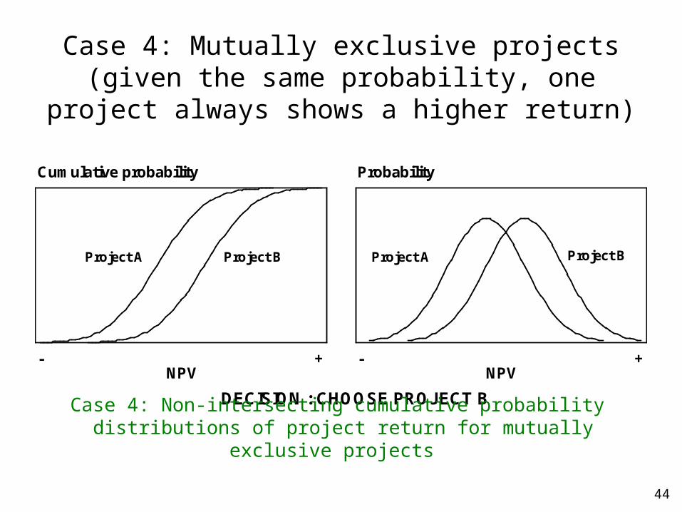
Case 4: Mutually exclusive projects(given the same probability, one project always shows a
higher return)
+-
Project A Project B
NPV+-
NPV
ProbabilityCumulative probability
DECISION : CHOOSE PROJECT B
Project A Project B
Case 4: Non‑intersecting cumulative probability distributions of project return for mutually exclusive projects

45
Case 5: Mutually exclusive projects (high return vs. low loss)
Case 5: Intersecting cumulative probability distributions of project return for mutually exclusive projects
+-
Project A Project B
NPV+-
NPV
ProbabilityCumulative probability
DECISION : INDETERMINATE
Project A Project B
46
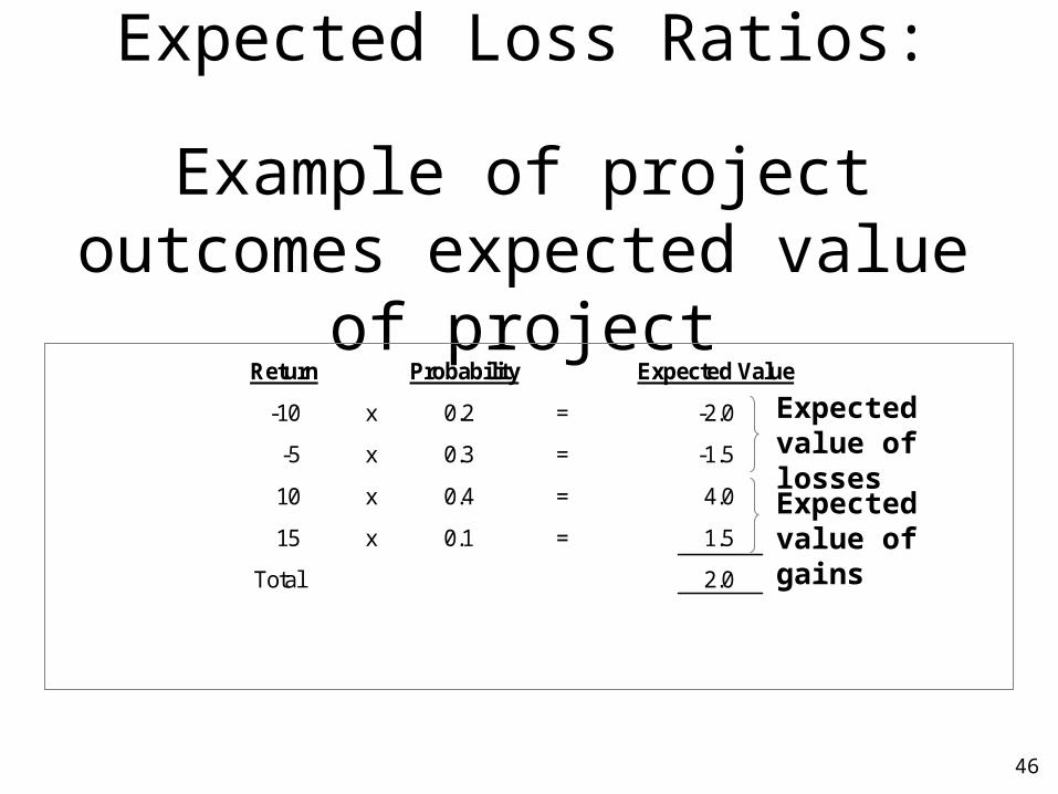
Expected Loss Ratios:
Example of project outcomes expected value of project
Return Probability Expected Value
-10 x 0.2 = -2.0
-5 x 0.3 = -1.5
10 x 0.4 = 4.0
15 x 0.1 = 1.5
Total 2.0
Expected value of losses
Expected value of gains
47
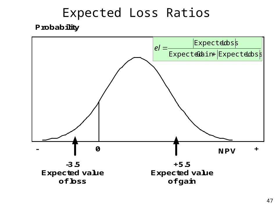
Expected Loss Ratios
+- 0 NPV
Probability
-3.5Expected value
of loss
+5.5Expected value
of gain
Loss ExpectedGain Expected
Loss Expected
el
48
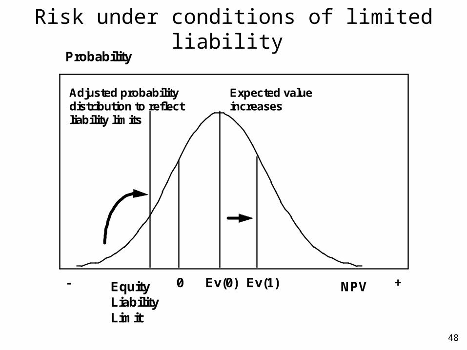
Risk under conditions of limited liability
+- Ev(1)Ev(0)0 NPV
Probability
EquityLiabilityLimit
Expected valueincreases
Adjusted probabilitydistribution to reflectliability limits
49
Advantages of risk analysis
• It enhances decision making on marginal projects.
• It screens new project ideas and aids the identification of investment opportunities.
• It highlights project areas that need further investigation and guides the collection of information.
• It aids the reformulation of projects to suit the attitudes and requirements of the investor.
• It induces the careful re‑examination of the single‑value estimates in the deterministic appraisal.
• It helps reduce project evaluation bias through eliminating the need to resort to conservative estimates.

50
• It facilitates the thorough use of experts.
• It bridges the communication gap between the analyst and the decision maker.
• It supplies a framework for evaluating project result estimates.
• It provides the necessary information base to facilitate a more efficient allocation and management of risk among various parties involved in a project.
• It makes possible the identification and measurement of explicit liquidity and repayment problems in terms of time and probability that these may occur during the life of the project.
Advantages of risk analysis (cont.)
51
Finally two words of caution:• Overlooking significant inter-relationships among the
projected variables can distort the results of risk analysis and lead to misleading conclusions.
• The accuracy of the results of risk analysis can only be as good as the predictive capacity of the model employed.

52
Lecture on Crystal Ball
FINA 522: Project Finance and Risk Management

INTRODUCTION TO RISK ANALYSIS PROGRAM
MICROSOFT EXCEL& CRYSTAL BALL

INTRODUCTION TO RISK ANALYSIS PROGRAM
MICROSOFT EXCEL& CRYSTAL BALL
June 2006
55
WHY do we need Risk Analysis ?
• Project returns are spread over time, therefore are subject to risk as they are the result of many uncertain events.
• Each variable affecting NPV is subject to high level of uncertainty
• Need to reduce the likelihood to undertake a "bad" project while not failing to accept a "good" project
Crystal ball risk software will help us
• identify, analyze, and interpret the expected variability in project outcomes.

56
WHAT CRYSTAL BALL SOFTWARE DOES?
• Traditionally it is the most likely outcome (mode) that
has been presented for decision making.
• Monte Carlo analysis enables one to estimate the
expected values of the outcome of our project.
• It also allows us to estimate the impact on the expected
value and standard deviation of the outcomes when
contracts and other risk management techniques are
applied to the project.

57
Methods
• Sensitivity Analysis
• Monte Carlo Risk Analysis (or Simulation
Analysis) using Crystal Ball Software
58
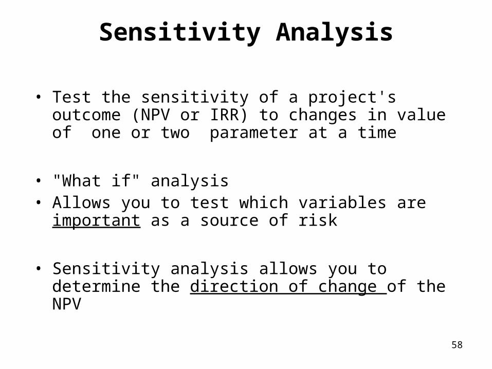
Sensitivity Analysis
• Test the sensitivity of a project's outcome (NPV or IRR) to changes in value of one or two parameter at a time
• "What if" analysis• Allows you to test which variables are important as a
source of risk
• Sensitivity analysis allows you to determine the direction of change of the NPV
59
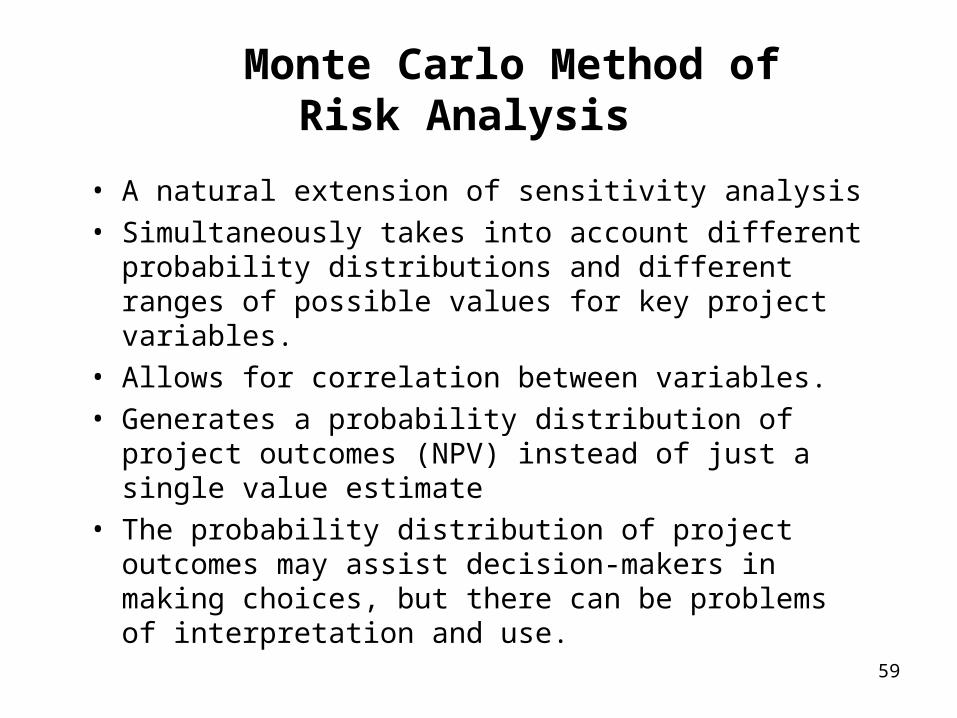
Monte Carlo Method of Risk Analysis
• A natural extension of sensitivity analysis• Simultaneously takes into account different
probability distributions and different ranges of possible values for key project variables.
• Allows for correlation between variables.• Generates a probability distribution of project
outcomes (NPV) instead of just a single value estimate
• The probability distribution of project outcomes may assist decision-makers in making choices, but there can be problems of interpretation and use.
60
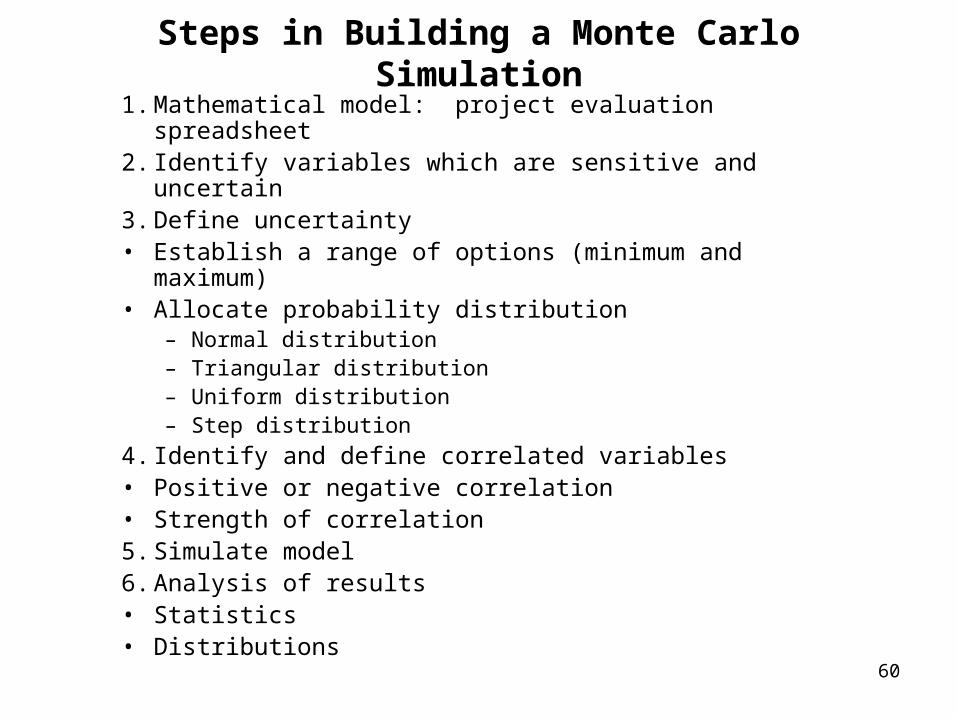
Steps in Building a Monte Carlo Simulation
1. Mathematical model: project evaluation spreadsheet2. Identify variables which are sensitive and uncertain3. Define uncertainty• Establish a range of options (minimum and maximum)• Allocate probability distribution
– Normal distribution– Triangular distribution– Uniform distribution– Step distribution
4. Identify and define correlated variables• Positive or negative correlation• Strength of correlation5. Simulate model6. Analysis of results• Statistics• Distributions
61
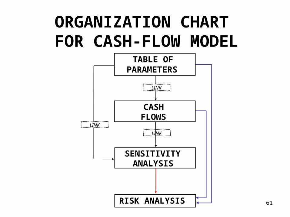
ORGANIZATION CHART FOR CASH-FLOW MODEL
TABLE OFPARAMETERS
CASHFLOWS
SENSITIVITYANALYSIS
LINK
LINK
LINK
RISK ANALYSIS
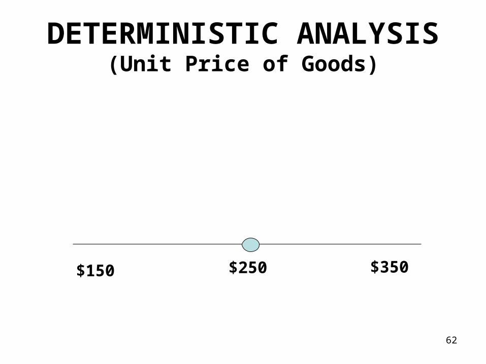
62
DETERMINISTIC ANALYSIS(Unit Price of Goods)
$250 $350$150
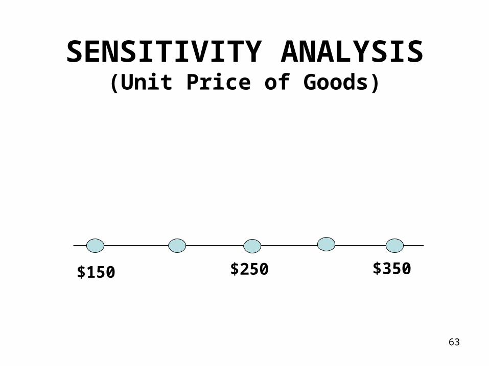
63
SENSITIVITY ANALYSIS(Unit Price of Goods)
$250 $350$150
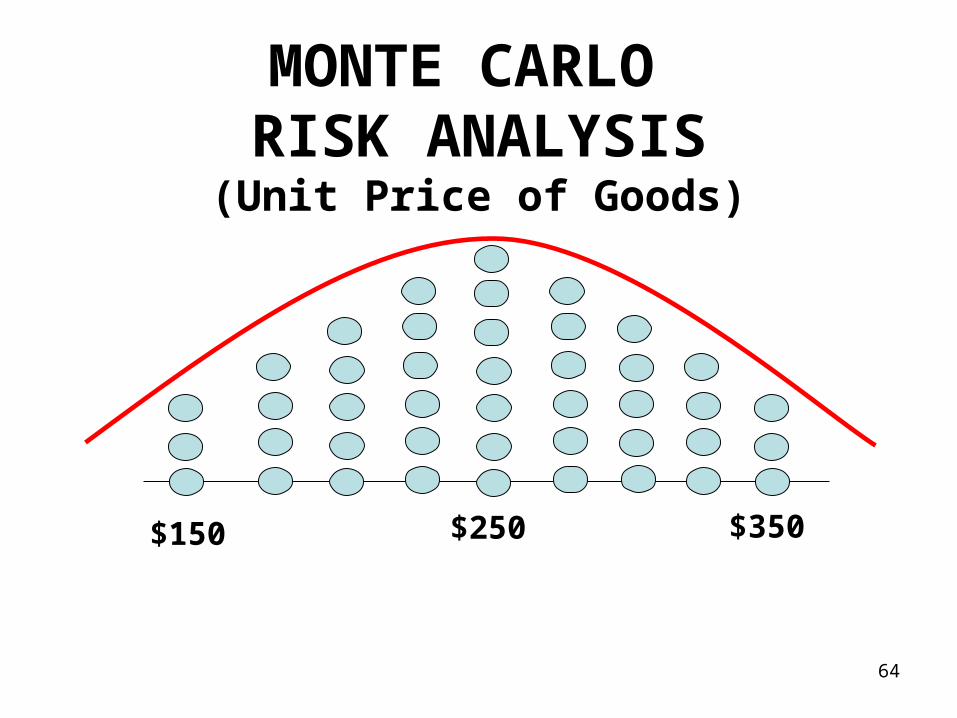
64
MONTE CARLO RISK ANALYSIS(Unit Price of Goods)
$250 $350$150

Upgrading a Gravel Road to Tar
Risk Analysis
Guidelines for Crystal Ball©

66
Steps to Follow:Step 1: Complete Financial Analysis
Step 2: Identify “Risk Assumptions” and “Risk Forecasts”
Step 3: Choose a Probability Distribution and Correlations for Risk Assumptions
Step 4: Define Risk Assumptions and Correlations
Step 5: Define Risk Forecasts
Step 6: Configure Risk Simulation
Step 7: Running a Risk Simulation
Step 8: Prepare a Risk Report
Step 9: Interpretation of Results
67
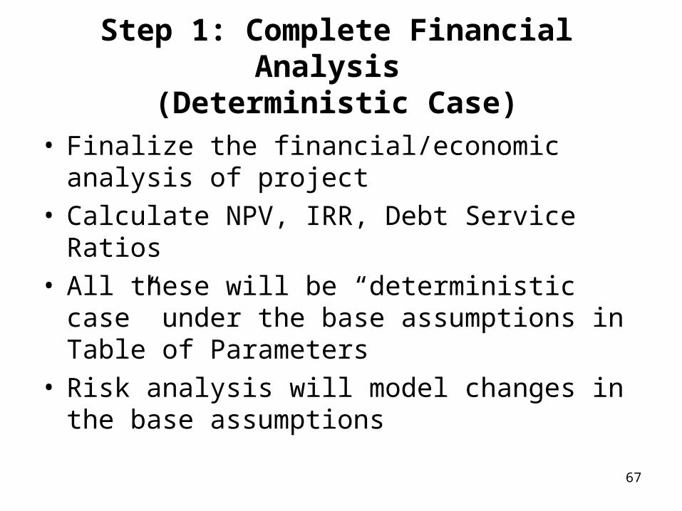
Step 1: Complete Financial Analysis (Deterministic Case)
• Finalize the financial/economic analysis of project
• Calculate NPV, IRR, Debt Service Ratios• All these will be “deterministic case” under the
base assumptions in Table of Parameters• Risk analysis will model changes in the base
assumptions
68
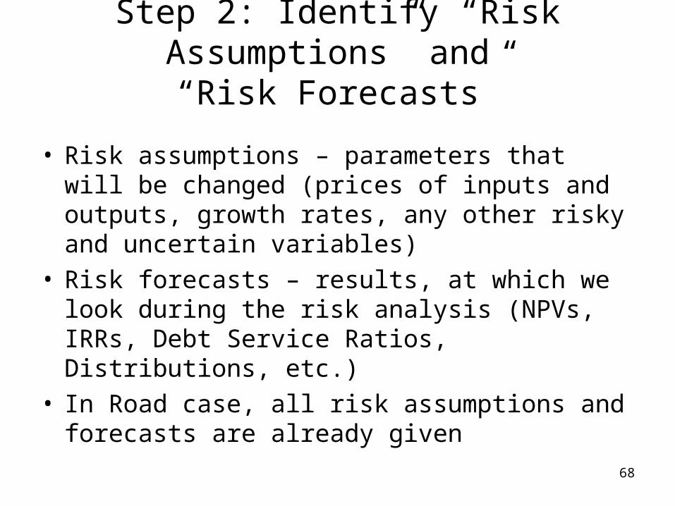
Step 2: Identify “Risk Assumptions” and
“Risk Forecasts”
• Risk assumptions – parameters that will be changed (prices of inputs and outputs, growth rates, any other risky and uncertain variables)
• Risk forecasts – results, at which we look during the risk analysis (NPVs, IRRs, Debt Service Ratios, Distributions, etc.)
• In Road case, all risk assumptions and forecasts are already given
69
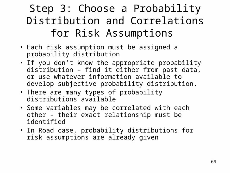
Step 3: Choose a Probability Distribution and Correlations for Risk Assumptions
• Each risk assumption must be assigned a probability distribution
• If you don’t know the appropriate probability distribution – find it either from past data, or use whatever information available to develop subjective probability distribution.
• There are many types of probability distributions available • Some variables may be correlated with each other – their
exact relationship must be identified• In Road case, probability distributions for risk
assumptions are already given
70
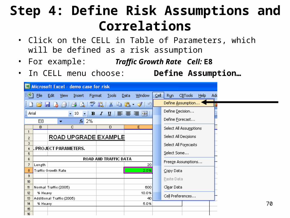
Step 4: Define Risk Assumptions and Correlations
• Click on the CELL in Table of Parameters, which will be defined as a risk assumption
• For example: Traffic Growth Rate Cell: E8
• In CELL menu choose: Define Assumption…
71
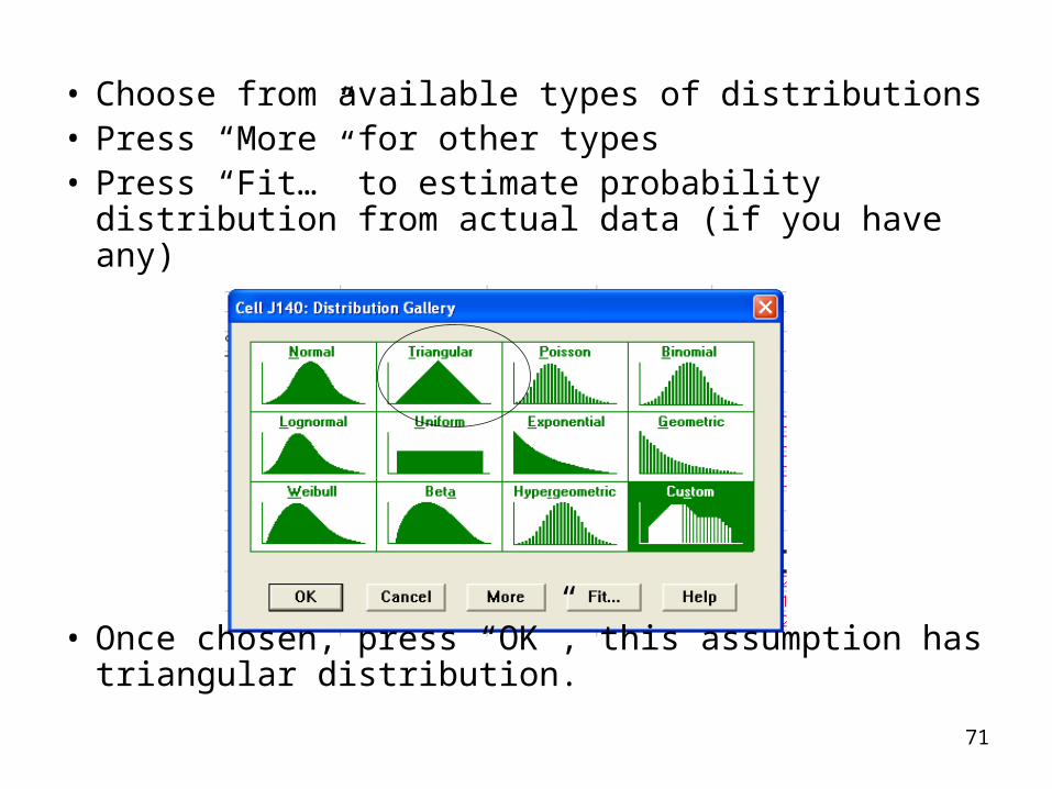
• Choose from available types of distributions• Press “More” for other types• Press “Fit…” to estimate probability distribution
from actual data (if you have any)
• Once chosen, press “OK”, this assumption has triangular distribution.

72
• Insert the distribution as given.• For example: Traffic Growth Rate Cell E8 (Triangular)
Assumption Name
Mean(Likeliest)
Minimum Value Maximum Value
• Insert the distribution as given Minimum 0.00 Likeliest 0.04 Maximum 0.08

73
• For triangular distribution, fill-in:
– Assumption Name– Minimum and Maximum Values– Press “Enter” to update display
• Press “OK” (risk assumption is defined)
74
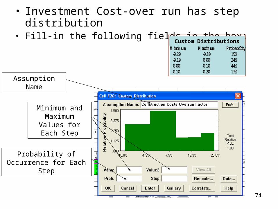
• Investment Cost-over run has step distribution• Fill-in the following fields in the box:
Minimum and Maximum Values
for Each Step
Assumption Name
Probability of Occurrence for Each Step
Custom DistributionsMinimum Maximum Probability -0.20 -0.10 19% -0.10 0.00 24% 0.00 0.10 44% 0.10 0.20 13%
75
• For custom distribution, fill-in:
– Assumption Name– Minimum and Maximum Values for a Step– Probability of Occurrence for that Step– Press “Enter” to update display– Continue with other steps
• Finally, press “OK” (risk assumption is defined)
• Note: if mistakenly entered, steps can be edited later by clicking on them, changing to new values and pressing “Enter” and then “OK”.

76
• Maintenance Costs Savings Factor has triangular• Continue with ALL other assumptions• For example: Maintenance Costs Savings Factor (Triangular)
Assumption Name
Mean
Minimum Value
Maximum Value
Minimum -0.10 Likeliest 0.00 Maximum 0.10
Triangular Distribution

77
• This example shows, how to define the correlation between two variables.
• In this assignment, we assume that traffic growth rate and the maintenance costs saving factor have correlation coefficient of -0.6
• Click on the value which have correlation then go to the define assumption
• Press “Correlate…” in the assumption of maintenance costs saving factor

78
• After click on the correlation, the following screen appears.
Correlation Coefficient
Assumption Name
• Press “Select Assumption” (in this case Traffic Growth Rate)
• Fill-in the correlation coefficient (in this case -0.6)
• Press “Enter” to update display
• Repeat procedure for all assumptions being correlated
• Finally, press “OK” (correlations are defined)
• See the picture on the right.

79
• VOC Savings Factor has normal distribution• Continue with ALL other assumptions• For example: VOC Savings Factor Cell: F22 (Normal)
Assumption Name
Standard Deviation
Deterministic Value
Normal Distribution
Mean 0.00 Standard Dev. 0.12
80
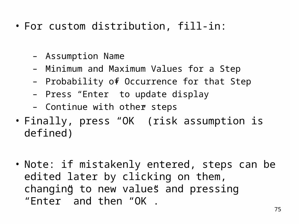
• Time Saving Factor has uniform distribution• Continue with ALL other assumptions• Some assumptions will have different probability distributions• For example: Time Saving Factor Cell: F23 (Uniform)
Assumption Name
Minimum Value
Maximum Value
Minimum -0.12 Maximum 0.12
Uniform Distribution
81
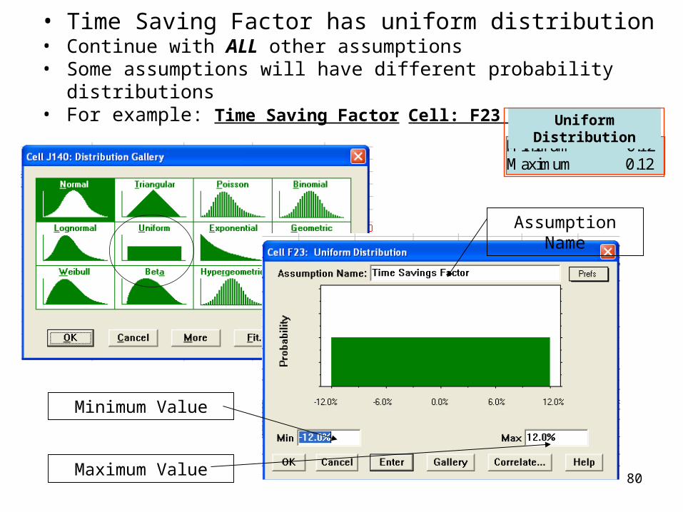
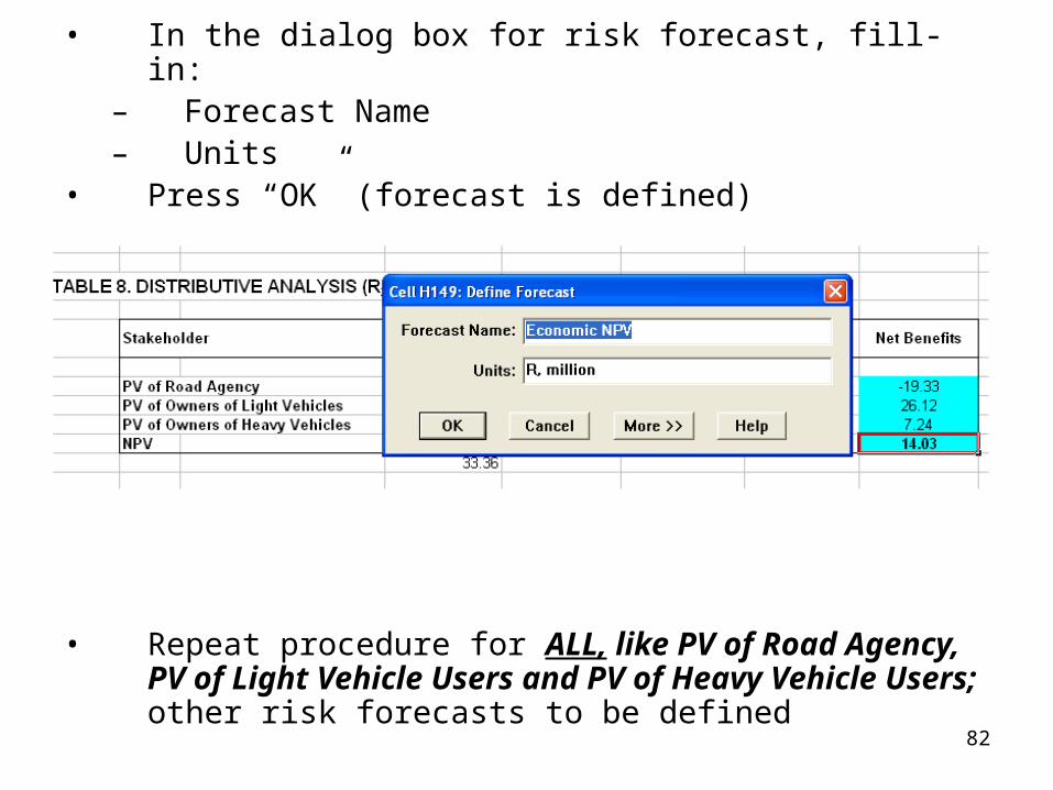
Step 5: Define Risk Forecasts
• Click on the CELL in spreadsheet, which will be defined as a risk forecast
• For example: NPV (Economic) H149• In CELL menu choose: Define Forecast…
82
• In the dialog box for risk forecast, fill-in:– Forecast Name– Units
• Press “OK” (forecast is defined)
• Repeat procedure for ALL, like PV of Road Agency, PV of Light Vehicle Users and PV of Heavy Vehicle Users; other risk forecasts to be defined
83
NOTES TO ADVANCED USER• Parameters of risk assumptions and forecasts can
be copied by special Crystal Ball copy-paste commands
• This saves time and effort in repeated tasks (e.g. defining yearly inflation rate)
• Select the cell from which you want to copy risk parameters --> in CELL menu choose COPY DATA
• Select the cell to which the risk parameters are applied --> in CELL menu choose PASTE DATA
• ALL risk parameters can be removed in a cell by choosing CELL menu – CLEAR DATA
84
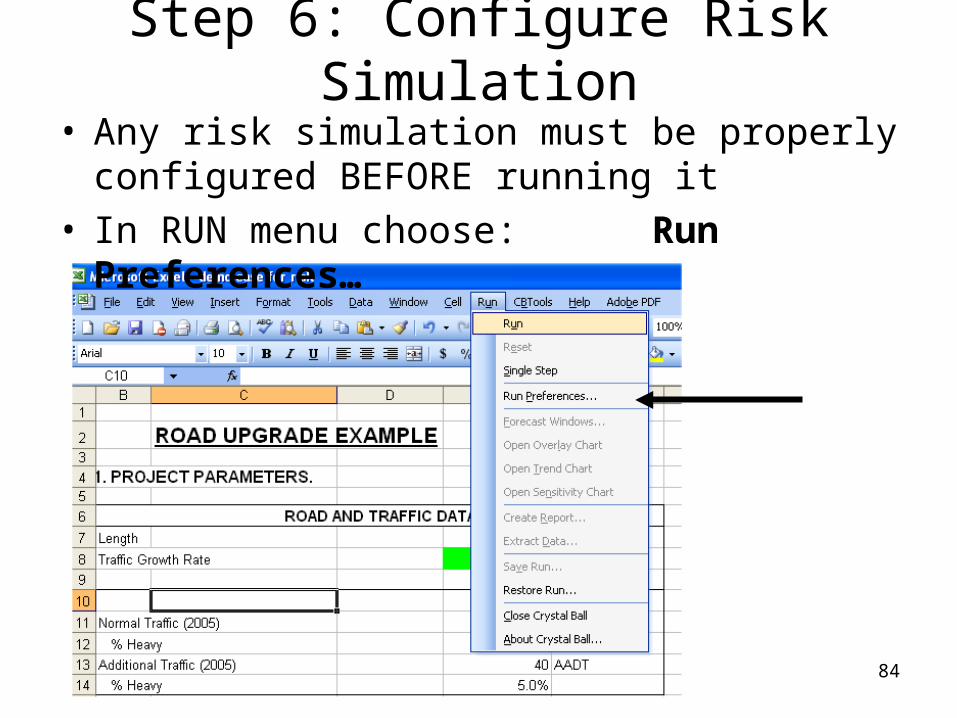
Step 6: Configure Risk Simulation
• Any risk simulation must be properly configured BEFORE running it
• In RUN menu choose: Run Preferences…

85
• Set the necessary Number of Trials (5,000 runs is usually considered to be sufficient)
• Switch OFF the following:– Stop if specified precision is reached; and– Stop if calculation error occurs
• Press “>>” to go to next stage …
Set Number of Trials
Switch OFF
Got to NEXT stage

86
• Choose Sampling Method:– Monte Carlo (most often used)– Latin Hypercube (computer memory intensive)
• Do NOT change any other parameters here
• Press “>>” to go to next stage …
Sampling Method

87
• Do NOT change Use Burst Mode When Idle• Select one of the options in Minimize While
Running:– All Spreadsheets (recommended)
• Switch ON the option of Suppress Forecast Windows
• Press “OK” (configuration is complete)
Speed Options
Switch ON
88
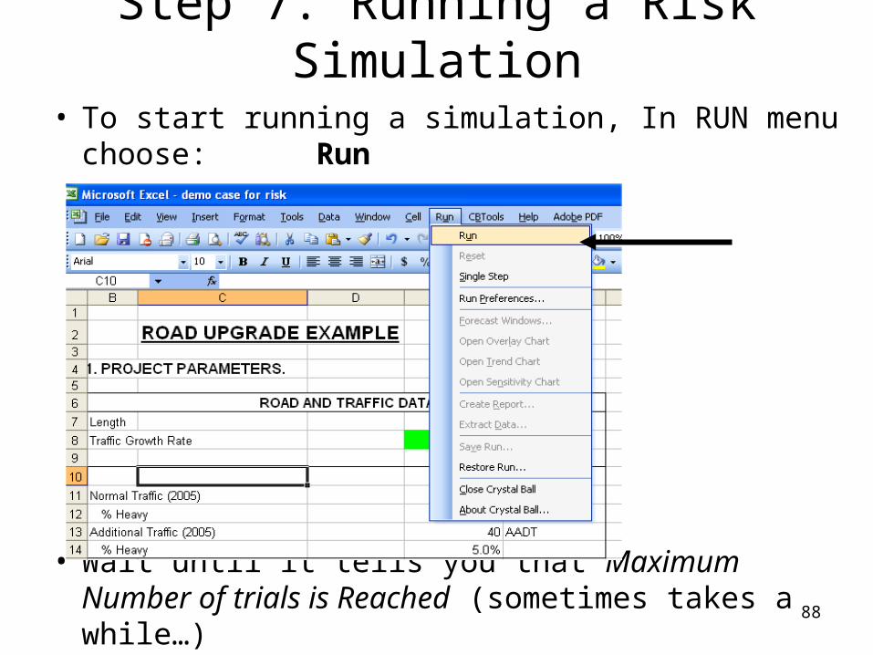
Step 7: Running a Risk Simulation
• To start running a simulation, In RUN menu choose: Run
• Wait until it tells you that Maximum Number of trials is Reached (sometimes takes a while…)
89
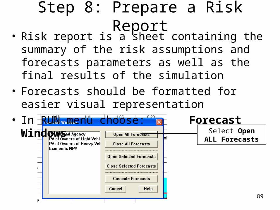
Step 8: Prepare a Risk Report• Risk report is a sheet containing the summary of
the risk assumptions and forecasts parameters as well as the final results of the simulation
• Forecasts should be formatted for easier visual representation
• In RUN menu choose: Forecast Windows
Select Open ALL Forecasts

90
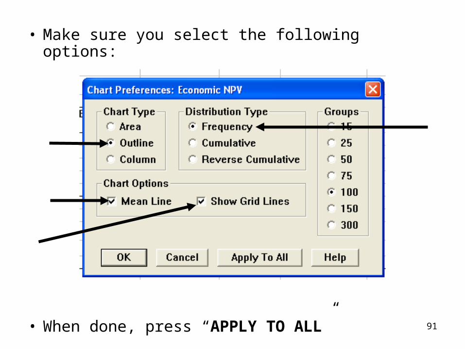
• In the forecast window, choose PREFERENCES menu and select CHART…
91
• Make sure you select the following options:
• When done, press “APPLY TO ALL”
92
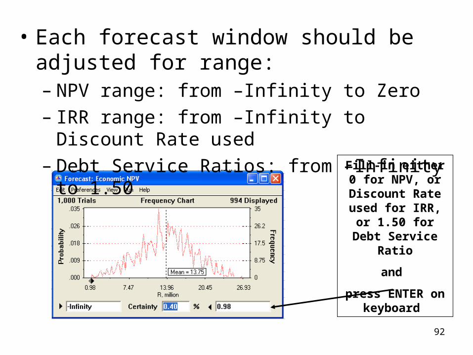
• Each forecast window should be adjusted for range:– NPV range: from –Infinity to Zero– IRR range: from –Infinity to Discount Rate used– Debt Service Ratios: from –Infinity to 1.50
Fill-in either 0 for NPV, or Discount Rate used for IRR,
or 1.50 for Debt Service Ratio
and
press ENTER on keyboard
93
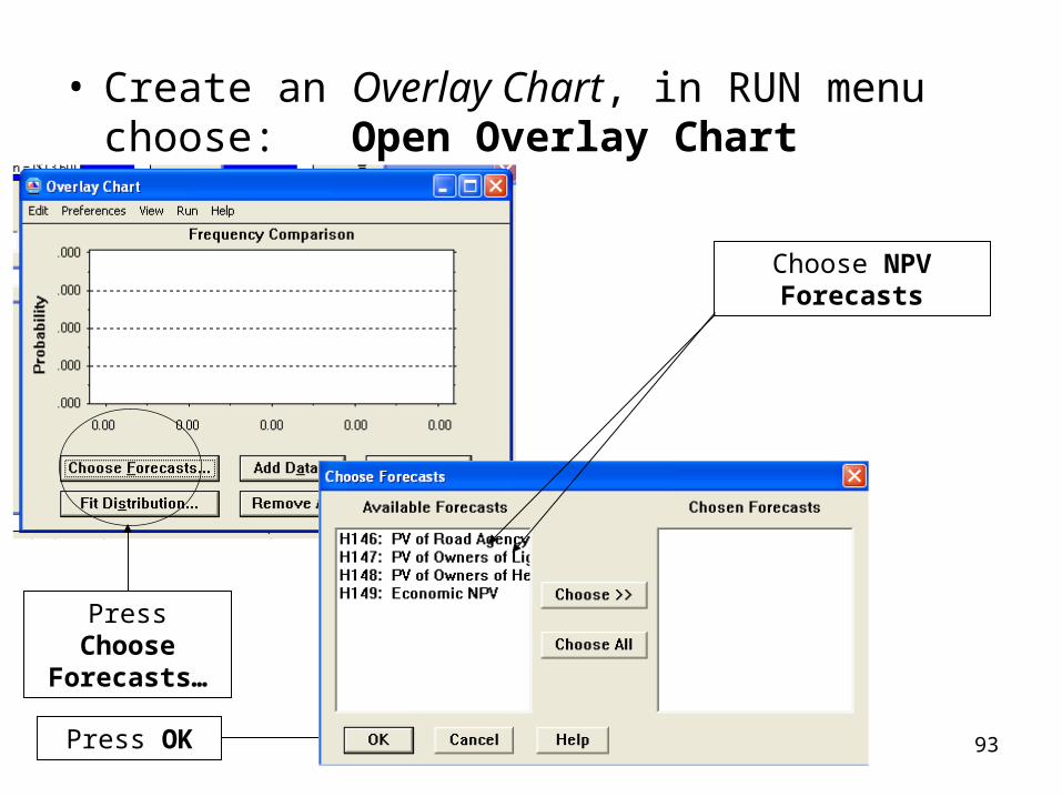
• Create an Overlay Chart, in RUN menu choose: Open Overlay Chart
Press Choose Forecasts…
Choose NPV Forecasts
Press OK

94
• Overlay chart should be also formatted for better visual presentation, as shown below:
Press Chart Prefs…
Press OK
95
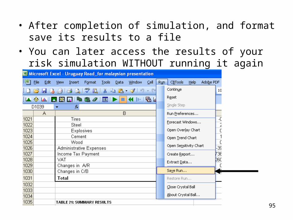
• After completion of simulation, and format save its results to a file
• You can later access the results of your risk simulation WITHOUT running it again
96
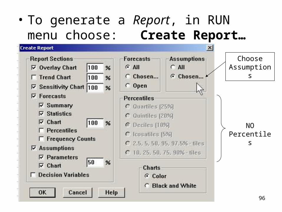
• To generate a Report, in RUN menu choose: Create Report…
Choose Assumptions
NO Percentiles

97
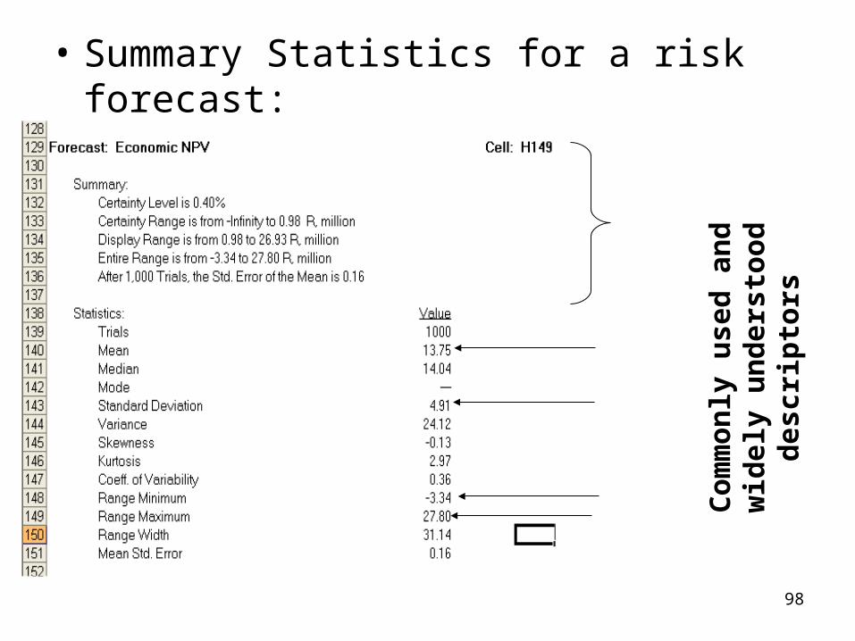
Step 9: Interpretation of Results
• Analyze the results, which will be presented by:– Overlay Chart (comparison of several NPVs)– Forecast Charts for each risk forecast (NPVs, IRR,
Debt Service Ratios)
• Summary Statistics for each risk forecast• Risk results must be compared with the
results of deterministic analysis
98
• Summary Statistics for a risk forecast:
Co
mm
on
ly u
sed
an
d w
idel
y u
nd
erst
oo
d d
escr
ipto
rs

99
• What do we need to do to manage risks?
• Is risk management proposal effective? – Need to test contracts.