


Languages
Pages
Legal


Unsolved Problems in Dark Energya.k.a. Everything
Wayne HuBenasque, February 2011

Said the great Spanish physicist Raul Jimenez (in Americanized paraphrase):
“Better Lame than Late”
– circa 24 hrs ago

Said the great Spanish physicist Raul Jimenez (in Americanized paraphrase):
or the A delayed Session = Cut the F***ing Time correspondence
“Better Lame than Late”
– circa 24 hrs ago

Prolific Participants: p+p→? Hitoshi says 2 in billion survive! [1] S. A. Thomas, F. B. Abdalla, and O. Lahav, (2010), arXiv:1012.2272 [astro-ph.CO] .
[2] S. A. Thomas, F. B. Abdalla, and O. Lahav, (2010), arXiv:1011.2448 [astro-ph.CO] .
[3] B. Joachimi, R. Mandelbaum, F. Abdalla, and S. Bridle, (2010), arXiv:1008.3491 [astro-ph.CO] .
[4] A. Cooray, S. Eales, S. Chapman, D. L. Clements, O. Dore, et al., (2010), arXiv:1007.3519 [astro-ph.CO] .
[5] E. Cypriano, A. Amara, L. Voigt, S. Bridle, F. Abdalla, et al., (2010), arXiv:1001.0759 [astro-ph.CO] .
[6] U. Sawangwit, T. Shanks, F. Abdalla, R. Cannon, S. Croom, et al., (2009), arXiv:0912.0511 [astro-ph.CO] .
[7] R. Mandelbaum, C. Blake, S. Bridle, F. B. Abdalla, S. Brough, et al., (2009), arXiv:0911.5347 [astro-ph.CO] .
[8] F. B. Abdalla, C. Blake, and S. Rawlings, (2009), arXiv:0905.4311 [astro-ph.CO] .
[9] S. T. Myers, F. B. Abdalla, C. Blake, L. Koopmans, J. Lazio, et al., (2009), arXiv:0903.0615 [astro-ph.CO] .
[10] S. A. Thomas, F. B. Abdalla, and J. Weller, Mon.Not.Roy.Astron.Soc., 395, 197 (2009), arXiv:0810.4863 [astro-ph] .
[11] A. Amara and T. Kitching, (2010), arXiv:1009.3274 [astro-ph.CO] .
[12] T. Kitching, A. Amara, M. Gill, S. Harmeling, C. Heymans, et al., (2010), arXiv:1009.0779 [astro-ph.CO] .
[13] S. Pires and A. Amara, Astrophys.J., 723, 1507 (2010), arXiv:1009.0712 [astro-ph.CO] .
[14] R. Metcalf and A. Amara, (2010), arXiv:1007.1599 [astro-ph.CO] .
[15] A. Refregier, A. Amara, T. Kitching, A. Rassat, R. Scaramella, et al., (2010), arXiv:1001.0061 [astro-ph.IM] .
[16] I. Debono, A. Rassat, A. Refregier, A. Amara, and T. Kitching, (2009), arXiv:0911.3448 [astro-ph.CO] .
[17] R. Bordoloi, S. J. Lilly, and A. Amara, (2009), arXiv:0910.5735 [astro-ph.CO] .
[18] D. Bacon, A. Amara, and J. Read, (2009), arXiv:0909.5133 [astro-ph.CO] .
[19] J. Berge, A. Amara, and A. Refregier, Astrophys.J., 712, 992 (2010), arXiv:0909.0529 [astro-ph.CO] .
[20] S. Bridle, S. T. Balan, M. Bethge, M. Gentile, S. Harmeling, et al., (2009), arXiv:0908.0945 [astro-ph.CO] .
[21] T. Kitching and A. Amara, (2009), arXiv:0905.3383 [astro-ph.CO] .
[22] A. Amara, A. Refregier, and S. Paulin-Henriksson, (2009), arXiv:0905.3176 [astro-ph.CO] .
[23] S. Pires, J.-L. Starck, A. Amara, A. Refregier, and R. Teyssier, AIP Conf.Proc., 1241, 1118 (2010), arXiv:0904.2995 [astro-ph.CO] .
[24] S. Paulin-Henriksson, A. Refregier, and A. Amara, (2009), arXiv:0901.3557 [astro-ph.IM] .
[25] T. Kitching, A. Amara, A. Rassat, and A. Refregier, (2009), arXiv:0901.3143 [astro-ph.IM] .

[26] A. Avgoustidis, L. Verde, and R. Jimenez, JCAP, 0906, 012 (2009), arXiv:0902.2006 [astro-ph.CO] .
[27] E. J. Copeland, AIP Conf.Proc., 1241, 125 (2010).
[28] S.-Y. Zhou, E. J. Copeland, and P. M. Saffin, JCAP, 0907, 009 (2009), arXiv:0903.4610 [gr-qc] .
[29] A. Heavens, Nucl.Phys.Proc.Suppl., 194, 76 (2009), arXiv:0911.0350 [astro-ph.CO] .
[30] D. E. Holz and S. Perlmutter, (2010), arXiv:1004.5349 [astro-ph.CO] .
[31] C. M. Hirata, D. E. Holz, and C. Cutler, Phys.Rev., D81, 124046 (2010), arXiv:1004.3988 [astro-ph.CO] .
[32] D. Sarkar, S. Sullivan, S. Joudaki, A. Amblard, A. Cooray, et al., Nucl.Phys.Proc.Suppl., 194, 307 (2009).
[33] P. Serra, A. Cooray, D. E. Holz, A. Melchiorri, S. Pandolfi, et al., Phys.Rev., D80, 121302 (2009), arXiv:0908.3186 [astro-ph.CO] .
[34] C. Cutler and D. E. Holz, Phys.Rev., D80, 104009 (2009), arXiv:0906.3752 [astro-ph.CO] .
[35] S. Joudaki, A. Cooray, and D. E. Holz, Phys.Rev., D80, 023003 (2009), arXiv:0904.4697 [astro-ph.CO] .
[36] A. R. Cooray, D. E. Holz, and R. Caldwell, JCAP, 1011, 015 (2010), arXiv:0812.0376 [astro-ph] .
[37] B. Hoyle, R. Jimenez, and L. Verde, (2010), arXiv:1009.3884 [astro-ph.CO] .
[38] C. Shapiro, S. Dodelson, B. Hoyle, L. Samushia, and B. Flaugher, Phys.Rev., D82, 043520 (2010), arXiv:1004.4810 [astro-ph.CO] .
[39] L. L. Honorez, B. A. Reid, O. Mena, L. Verde, and R. Jimenez, JCAP, 1009, 029 (2010), arXiv:1006.0877 [astro-ph.CO] .
[40] S. Ferraro, F. Schmidt, and W. Hu, (2010), arXiv:1011.0992 [astro-ph.CO] .
[41] M. J. Mortonson, W. Hu, and D. Huterer, Phys.Rev., D83, 023015 (2011), arXiv:1011.0004 [astro-ph.CO] .
[42] S. S. Seahra and W. Hu, Phys.Rev., D82, 124015 (2010), arXiv:1007.4242 [astro-ph.CO] .
[43] M. J. Mortonson, D. Huterer, and W. Hu, Phys.Rev., D82, 063004 (2010), arXiv:1004.0236 [astro-ph.CO] .
[44] L. Lombriser, A. Slosar, U. Seljak, and W. Hu, (2010), arXiv:1003.3009 [astro-ph.CO] .
[45] M. J. Mortonson and W. Hu, Phys.Rev., D81, 067302 (2010), arXiv:1001.4803 [astro-ph.CO] .
[46] M. J. Mortonson, W. Hu, and D. Huterer, Phys.Rev., D81, 063007 (2010), arXiv:0912.3816 [astro-ph.CO] .
[47] F. Schmidt, W. Hu, and M. Lima, Phys.Rev., D81, 063005 (2010), arXiv:0911.5178 [astro-ph.CO] .
[48] F. Schmidt, A. Vikhlinin, and W. Hu, Phys.Rev., D80, 083505 (2009), arXiv:0908.2457 [astro-ph.CO] .
[49] M. Mortonson, W. Hu, and D. Huterer, Phys.Rev., D80, 067301 (2009), arXiv:0908.1408 [astro-ph.CO] .
[50] W. Hu, Nucl.Phys.Proc.Suppl., 194, 230 (2009), arXiv:0906.2024 [astro-ph.CO] .
[51] A. Upadhye and W. Hu, Phys.Rev., D80, 064002 (2009), arXiv:0905.4055 [astro-ph.CO] .
[52] L. Lombriser, W. Hu, W. Fang, and U. Seljak, Phys.Rev., D80, 063536 (2009), arXiv:0905.1112 [astro-ph.CO] .

[53] T. Kitching and A. Taylor, (2010), arXiv:1012.3479 [astro-ph.CO] .
[54] D. Munshi, T. Kitching, A. Heavens, and P. Coles, (2010), arXiv:1012.3658 [astro-ph.CO] .
[55] S. Ilic, M. Kunz, A. R. Liddle, and J. A. Frieman, Phys.Rev., D81, 103502 (2010), arXiv:1002.4196 [astro-ph.CO] .
[56] C. Gao, M. Kunz, A. R. Liddle, and D. Parkinson, Phys.Rev., D81, 043520 (2010), arXiv:0912.0949 [astro-ph.CO] .
[57] M. Kunz, A. R. Liddle, D. Parkinson, and C. Gao, Phys.Rev., D80, 083533 (2009), arXiv:0908.3197 [astro-ph.CO] .
[58] D. Parkinson, M. Kunz, A. R. Liddle, B. A. Bassett, R. C. Nichol, et al., (2009), arXiv:0905.3410 [astro-ph.CO] .
[59] G. Caldera-Cabral, R. Maartens, and L. Urena-Lopez, AIP Conf.Proc., 1241, 741 (2010).
[60] C. Clarkson and R. Maartens, Class.Quant.Grav., 27, 124008 (2010), arXiv:1005.2165 [astro-ph.CO] .
[61] R. Maartens and K. Koyama, Living Rev.Rel., 13, 5 (2010), arXiv:1004.3962 [hep-th] .
[62] E. Majerotto, J. Valiviita, and R. Maartens, Nucl.Phys.Proc.Suppl., 194, 260 (2009).
[63] C. G. Boehmer, G. Caldera-Cabral, N. Chan, R. Lazkoz, and R. Maartens, Phys.Rev., D81, 083003 (2010), arXiv:0911.3089 [gr-qc] .
[64] J. Valiviita, R. Maartens, and E. Majerotto, Mon.Not.Roy.Astron.Soc., 402, 2355 (2010), arXiv:0907.4987 [astro-ph.CO] .
[65] E. Majerotto, J. Valiviita, and R. Maartens, Mon.Not.Roy.Astron.Soc., 402, 2344 (2010), arXiv:0907.4981 [astro-ph.CO] .
[66] C. Boehmer, G. Caldera-Cabral, R. Lazkoz, and R. Maartens, AIP Conf.Proc., 1122, 197 (2009).
[67] K. Koyama, R. Maartens, and Y.-S. Song, JCAP, 0910, 017 (2009), arXiv:0907.2126 [astro-ph.CO] .
[68] G. Caldera-Cabral, R. Maartens, and B. M. Schaefer, JCAP, 0907, 027 (2009), arXiv:0905.0492 [astro-ph.CO] .
[69] G. Caldera-Cabral, R. Maartens, and L. Urena-Lopez, Phys.Rev., D79, 063518 (2009), arXiv:0812.1827 [gr-qc] .
[70] D. Bertacca, A. Raccanelli, O. F. Piattella, D. Pietrobon, N. Bartolo, et al., (2011), arXiv:1102.0284 [astro-ph.CO] .
[71] O. Mena, J.Phys.Conf.Ser., 259, 012084 (2010).
[72] L. Lopez Honorez, O. Mena, and G. Panotopoulos, Phys.Rev., D82, 123525 (2010), arXiv:1009.5263 [astro-ph.CO] .
[73] R. Mainini and D. F. Mota, (2010), arXiv:1011.0083 [astro-ph.CO] .
[74] D. F. Mota and H. A. Winther, (2010), arXiv:1010.5650 [astro-ph.CO] .
[75] R. Gannouji, B. Moraes, D. F. Mota, D. Polarski, S. Tsujikawa, et al., Phys.Rev., D82, 124006 (2010), arXiv:1010.3769 [astro-ph.CO] .
[76] D. F. Mota, M. Sandstad, and T. Zlosnik, JHEP, 1012, 051 (2010), arXiv:1009.6151 [astro-ph.CO] .
[77] B. Li, D. F. Mota, and J. D. Barrow, Astrophys.J., 728, 109 (2011), arXiv:1009.1400 [astro-ph.CO] .
[78] P. Brax, C. van de Bruck, D. F. Mota, N. J. Nunes, and H. A. Winther, Phys.Rev., D82, 083503 (2010), arXiv:1006.2796 [astro-ph.CO] .
[79] A. De Felice, D. F. Mota, and S. Tsujikawa, Mod.Phys.Lett., A25, 885 (2010).

[80] M. Zumalacarregui, T. Koivisto, D. Mota, and P. Ruiz-Lapuente, JCAP, 1005, 038 (2010), arXiv:1004.2684 [astro-ph.CO] .
[81] C. G. Boehmer, J. Burnett, D. F. Mota, and D. J. Shaw, JHEP, 1007, 053 (2010), arXiv:1003.3858 [hep-th] .
[82] A. De Felice, D. F. Mota, and S. Tsujikawa, Phys.Rev., D81, 023532 (2010), arXiv:0911.1811 [gr-qc] .
[83] N. Wintergerst, V. Pettorino, D. Mota, and C. Wetterich, Phys.Rev., D81, 063525 (2010), arXiv:0910.4985 [astro-ph.CO] .
[84] J. B. Jimenez, T. S. Koivisto, A. L. Maroto, and D. F. Mota, JCAP, 0910, 029 (2009), arXiv:0907.3648 [physics.gen-ph] .
[85] D. F. Mota and D. J. Shaw, EAS Publ.Ser., 36, 105 (2009).
[86] P. Creminelli, G. D’Amico, J. Norena, L. Senatore, and F. Vernizzi, JCAP, 1003, 027 (2010), arXiv:0911.2701 [astro-ph.CO] .
[87] P. Creminelli, G. D’Amico, J. Norena, and F. Vernizzi, JCAP, 0902, 018 (2009), arXiv:0811.0827 [astro-ph] .
[88] C. Deffayet, O. Pujolas, I. Sawicki, and A. Vikman, JCAP, 1010, 026 (2010), arXiv:1008.0048 [hep-th] .
[89] F. Simpson, Phys.Rev., D82, 083505 (2010), arXiv:1007.1034 [astro-ph.CO] .
[90] F. Simpson, B. M. Jackson, and J. A. Peacock, (2010), arXiv:1004.1920 [astro-ph.CO] .
[91] F. Simpson, Phys.Rev., D81, 043513 (2010), arXiv:0910.3836 [astro-ph.CO] .
[92] F. Simpson and J. A. Peacock, Phys.Rev., D81, 043512 (2010), arXiv:0910.3834 [astro-ph.CO] .
[93] F. Simpson, J. A. Peacock, and P. Simon, Phys.Rev., D79, 063508 (2009), arXiv:0901.3085 [astro-ph.CO] .
[94] C. Skordis and T. Zlosnik, (2011), arXiv:1101.6019 [gr-qc] .
[95] T. Clifton, M. Banados, and C. Skordis, Class.Quant.Grav., 27, 235020 (2010), arXiv:1006.5619 [gr-qc] .
[96] P. G. Ferreira and C. Skordis, Phys.Rev., D81, 104020 (2010), arXiv:1003.4231 [astro-ph.CO] .
[97] C. Skordis, Nucl.Phys.Proc.Suppl., 194, 332 (2009).
[98] C. Skordis, Nucl.Phys.Proc.Suppl., 194, 338 (2009).
[99] C. Skordis, Class.Quant.Grav., 26, 143001 (2009), arXiv:0903.3602 [astro-ph.CO] .
[100] A. Katz and R. Sundrum, JHEP, 0906, 003 (2009), arXiv:0902.3271 [hep-ph] .
[101] S. Bhattacharya, K. Heitmann, M. White, Z. Lukic, C. Wagner, et al., (2010), arXiv:1005.2239 [astro-ph.CO] .
[102] K. Heitmann, M. White, C. Wagner, S. Habib, and D. Higdon, Astrophys.J., 715, 104 (2010), arXiv:0812.1052 [astro-ph] .

Observational to Do List• Just 3 things (from a theorist’s perspective) 1. Falsify (flat) ΛCDM 2. Falsify (flat) ΛCDM 3. Falsify (flat) ΛCDM
ΛCDM

How to FalsifyTest the consistency of ΛCDM in parameter space
• Expand parameter space or take alternate models
• MCMC set of parameters, find evidence for tension with ΛCDM
• Good - well defined, optimal if models well motivated
• Bad - there are no well motivated alternatives to Λ (cf.Sundrum’s IQ Test)
• FOM (aka FML) and other elements of the Dark Energy Canon(Andrew Liddle and the New Bayesian Testament)
Test consistency in observable space
• MCMC in ΛCDM (or other complete paradigm likequintessence) and predict posteriors of new observables
• Good - theory says what best to observe to falsify ΛCDM
• Bad - falsify in favor of what?

Falsifying ΛCDM• Geometric measures of distance redshift from SN, CMB, BAO
Standard RulerSound Horizon
v CMB, BAO angularand redshift separation
Standard(izable) Candle
SupernovaeLuminosity v Flux

Cosmological Constant
Falsifying ΛCDM• Λ slows growth of structure in highly predictive way

Falsifiability of Smooth Dark Energy• With the smoothness assumption, dark energy only affects
gravitational growth of structure through changing the expansionrate
• Hence geometric measurements of the expansion rate predict thegrowth of structure
• Hubble Constant
• Supernovae
• Baryon Acoustic Oscillations
• Growth of structure measurements can therefore falsify the wholesmooth dark energy paradigm
• Cluster Abundance
• Weak Lensing
• Velocity Field (Redshift Space Distortion)

Mortonson, Hu, Huterer (2009)
QuintessenceCosmological Constant
Falsifying Quintessence• Dark energy slows growth of structure in highly predictive way
• Deviation significantly >2% rules out Λ with or without curvature
• Excess >2% rules out quintessence with or without curvature and early dark energy [as does >2% excess in H0]

Mortonson, Hu, Huterer (2009)
QuintessenceCosmological Constant
Dynamical Tests of Acceleration• Dark energy slows growth of structure in highly predictive way

Redshift Space Distortion• Redshift space distortions measure fG or fσ8 • Measurements in excess of ~5% of ΛCDM would rule out quintessence
Mortonson, Hu, Huterer (2009)
z z1 2 3 1
-0.4-0.05
0
0.05
0.10
-0.2
0
2 3
∆(fG
)/(fG
)
Cosmological Constant Quintessence

NonPC Caveats on PCs• Principal component decomposition of w(z) shows many components
can in principle be measured (Euclid, LSST, WFirst)• Yet even models like Albrecht-Skordis (oscillating w) are still
dominated by first component - average w or pivot - plus 1-2 weaker• Should a multidimensional parameterization be the basis for
optimizing an experiment?

Pink Elephant Parade• Too early too soon? SPT catalogue on 2500 sq degrees
Williamson et al (2010)
Other AnalysesHoyle, Jiminez, Verde (2010)many others...
Falisification CriteriaMortonson, Hu, Huterer (2010)Holz & Perlmutter (2010)

Systematics, Systematics, Systematics• E.g.: clusters - mass calibration from X-ray, SZ, optical, lensing

Systematics, Systematics, Systematics• Coffee talk: discuss amongst yourselves

Phenomenological To Do List• How best to parameterize consistency tests or define theoretically
predicted observables?
• How to treat baryonic effects in the non-linear regime e.g.• Galaxy occupation of halos [BAO, velocity field tests]• Concentration of clusters for cosmic shear
Extensive simulations + modelling of gastrophysics including starformation (see Brant, Licia, Volker’s talks)
• Calibrate non-linear mean and covariance of dark energyobservables as function of cosmological parameters (Volker’s talk)
• Simulate alternate models• (Kill) inhomogeneous models• Interacting dark matter-energy models• Modified gravity models

Modified Gravity = Dark Energy?• Solar system tests of gravity are informed by our knowledge of the
local stress energy content
• With no other constraint on the stress energy of dark energy otherthan conservation, modified gravity is formally equivalent to darkenergy
F (gµν) +Gµν = 8πGTMµν − F (gµν) = 8πGTDE
µν
Gµν = 8πG[TMµν + TDE
µν ]
and the Bianchi identity guarantees∇µTDEµν = 0
• Distinguishing between dark energy and modified gravity requiresclosure relations that relate components of stress energy tensor
• For matter components, closure relations take the form ofequations of state relating density, pressure and anisotropic stress

Modified Gravity 6= “Smooth DE”• Scalar field dark energy has δp = δρ (in constant field gauge) –
relativistic sound speed, no anisotropic stress
• Jeans stability implies that its energy density is spatially smoothcompared with the matter below the sound horizon
ds2 = −(1 + 2Ψ)dt2 + a2(1 + 2Φ)dx2
∇2(Φ−Ψ) ∝ matter density fluctuation
• Anisotropic stress changes the amount of space curvature per unitdynamical mass
∇2(Φ + Ψ) ∝ anisotropic stress
but its absence in a smooth dark energy model makesg = (Φ + Ψ)/(Φ−Ψ) = 0 for non-relativistic matter

Dynamical vs Lensing Mass• Newtonian potential: Ψ=δg00/2g00 which non-relativistic particles feel
• Space curvature: Φ=δgii/2gii which also deflects photons
• Most of the incisive tests of gravity reduce to testing the space curvature per unit dynamical mass

Lensing v Dynamical Comparison • Gravitational lensing around galaxies vs. linear velocity field (through redshift space distortions and galaxy autocorrelation)• Consistent with GR + smooth dark energy beginning to test interesting models
Zhang et al (2007); Jain & Zhang (2008)
Reyes et al (2010); Lombriser et al (2010)

Three Regimes• Three regimes with different dynamics
• Examples f(R) and DGP braneworld acceleration
• Parameterized Post-Friedmann description
• Non-linear regime return to General Relativity / Newtonian dynamics
r* rc
Scalar-TensorRegime
Conserved-CurvatureRegime
General RelativisticNon-Linear Regime
rhalos, galaxy large scale structure CMB

Three Regimes• Fully worked f(R) and DGP examples show 3 regimes
• Superhorizon regime: ζ =const., g(a)
• Linear regime - closure condition - analogue of “smooth” darkenergy density:
∇2(Φ−Ψ)/2 = −4πGa2∆ρ
g(a,x) ↔ g(a, k)
G can be promoted to G(a) but conformal invariance relatesfluctuations to field fluctuation that is small
• Non-linear regime:
∇2(Φ−Ψ)/2 = −4πGa2∆ρ
∇2Ψ = 4πGa2∆ρ− 1
2∇2φ

Nonlinear InteractionNon-linearity in the field equation
∇2φ = glin(a)a2 (8πG∆ρ−N [φ])
recovers linear theory if N [φ]→ 0
• For f(R), φ = fR and
N [φ] = δR(φ)
a non-linear function of the field
Llinked to gravitational potential
• For DGP, φ is the brane-bending mode and
N [φ] =r2c
a4
[(∇2φ)2 − (∇i∇jφ)2
]a non-linear function of second derivatives of the field
Linked to density fluctuation Example of Galileon invariance
Hu, Huterer & Smith (2006)
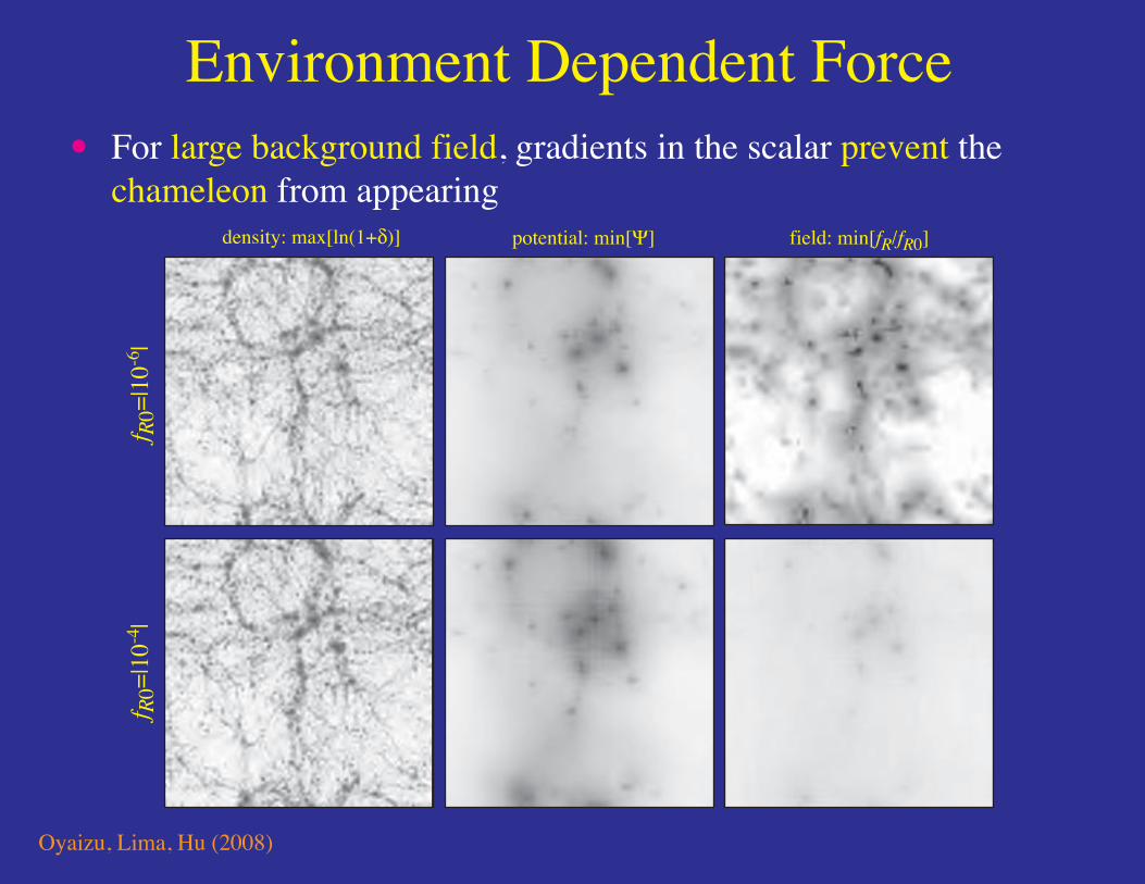
Environment Dependent ForceFor large background field, gradients in the scalar prevent the
chameleon from appearing
Oyaizu, Lima, Hu (2008)

Newtonian Potential Brane Bending Mode
DGP N-Body• DGP nonlinear derivative interaction solved by relaxation revealing the Vainshtein mechanism
Schmidt (2009); Chan & Scoccimarro (2009) (cf. Khoury & Wyman 2009)

Hu, L, Huterer & Smith (2006)
Mass FunctionEnhanced abundance of rare dark matter halos (clusters) with
extra force goes away as non-linearity increases
Schmidt, Lima, Oyaizu, Hu (2008)
Rel.
devi
atio
n dn/d
logM
M300 (h-1 M )

Phenomenological To Do List• How best to parameterize consistency tests or define theoretically
predicted observables?
• How to treat baryonic effects in the non-linear regime e.g.• Galaxy occupation of halos [BAO, velocity field tests]• Concentration of clusters for cosmic shear
Extensive simulations + modelling of gastrophysics including starformation (see Brant, Licia, Volker’s talks)
• Calibrate non-linear mean and covariance of dark energyobservables as function of cosmological parameters (Volker’s talk)
• Simulate alternate models• (Kill) inhomogeneous models• Interacting dark matter-energy models• Modified gravity models

Cooling/Star Formation in Clusters• Baryonic effects can lead to false falsfication of ΛCDM
Rudd, Zentner, Kravtsov (2007)
frac
tiona
l pow
er sp
ectru
m c
hang
e vs
Nbo
dy

Theoretical To Do List• Develop (discuss here) and explore known alternatives
• Dynamical Dark Energy
• Quintessence, k-essence, phantom, effective field theoreticquintessence, vanishing sound speed k-essence, extendedquintessence, coupled quintessence, electrostatic dark energy,elastically scattering dark energy, and other venial sins...
• Modified Gravity
• braneworld, f(R), f(G), cascading gravity, degravitation,galileon, massive gravity, kinetic gravity braiding, TeVeS andother heresies...
• Q: e.g. do massive gravity and galileon ideas forself-acceleration without ghosts make sense beyond thedecoupling limit

Theoretical To Do List• Develop alternatives that are more than just illustrative toy models
Floor is open to hear about them now!
• If observationally indistinguishable from Λ why does it have thevalue it does?
If we fail to find something to argue about in this session we canalways try landscape/anthropic

Andrew Liddle on Model Selection

ΛCDM: The current baseline cosmological model.
Parameterized dark energy models, eg CPL w = w0+(1-a) wa
The most common candidate alternative for dark energy studies.
Fundamental physics dark energy models, eg inverse power-laws, Albrecht-Skordis, etc
Many candidate models in the literature though many fail to fit current data. Not clear which are best motivated.
Modified gravity models
Determination of best candidate modified gravity models required.
Goal: to define the key model tests to be carried and, where possible, to optimize survey strategies to achieve them. First we need to figure out which are the interesting models.
What are we trying to achieve?

Parameter estimation testsWMAP 7-year Cosmological Interpretation 25
Fig. 13.— Joint two-dimensional marginalized constraint on thelinear evolution model of dark energy equation of state, w(a) =w0 + wa(1 ! a). The contours show the 68% and 95% CLfrom WMAP+H0+SN (red), WMAP+BAO+H0+SN (blue), andWMAP+BAO+H0+D!t+SN (black), for a flat universe.
When !k != 0, limits on w significantly weaken, witha tail extending to large negative values of w, unless su-pernova data are added.In Figure 12, we show that WMAP+BAO+H0
allows for w ! "2, which can be excludedby adding information on the time-delay distance.In both cases, the spatial curvature is well con-strained: we find !k = "0.0125+0.0064
!0.0067 from
WMAP+BAO+H0, and "0.0111+0.0060!0.0063 (68% CL) from
WMAP+BAO+H0+D!t, whose errors are comparableto that of the WMAP+BAO+H0 limit on !k with w ="1, !k = "0.0023+0.0054
!0.0056 (68% CL; see Section 4.3).However, w is poorly constrained: we find w =
"1.44 ± 0.27 from WMAP+BAO+H0, and "1.40 ±0.25 (68% CL) from WMAP+BAO+H0+D!t.Among the data combinations that do not use the in-
formation on the growth of structure, the most powerfulcombination for constraining !k and w simultaneouslyis a combination of the WMAP data, BAO (or D!t),and supernovae, as WMAP+BAO (or D!t) primarilyconstrains !k, and WMAP+SN primarily constrains w.With WMAP+BAO+SN, we find w = "0.999+0.057
!0.056 and!k = "0.0057+0.0066
!0.0068 (68% CL). Note that the errorin the curvature is essentially the same as that fromWMAP+BAO+H0, while the error in w is # 4 timessmaller.Vikhlinin et al. (2009b) combined their cluster abun-
dance data with the 5-year WMAP+BAO+SN to findw = "1.03 ± 0.06 (68% CL) for a curved universe.Reid et al. (2010a) combined their LRG power spectrumwith the 5-year WMAP data and the Union supernovadata to find w = "0.99 ± 0.11 and !k = "0.0109 ±0.0088 (68% CL). These results are in good agreementwith our 7-year WMAP+BAO+SN limit.
5.3. Time-dependent Equation of State
As for a time-dependent equation of state, we shall findconstraints on the present-day value of the equation of
state and its derivative using a linear form, w(a) = w0 +wa(1"a) (Chevallier & Polarski 2001; Linder 2003). Weassume a flat universe, !k = 0. (For recent limits on w(a)with !k != 0, see Wang 2009, and references therein.)While we have constrained this model using the WMAPdistance prior in the 5-year analysis (see Section 5.4.2of Komatsu et al. 2009a), in the 7-year analysis we shallpresent the full Markov Chain Monte Carlo explorationof this model.For a time-dependent equation of state, one must be
careful about the treatment of perturbations in dark en-ergy when w crosses"1. We use the “parametrized post-Friedmann” (PPF) approach, implemented in the CAMBcode following Fang et al. (2008).32
In Figure 13, we show the 7-year con-straints on w0 and wa from WMAP+H0+SN(red), WMAP+BAO+H0+SN (blue), andWMAP+BAO+H0+D!t+SN (black). The angulardiameter distances measured from BAO and D!t helpexclude models with large negative values of wa. We findthat the current data are consistent with a cosmologicalconstant, even when w is allowed to depend on time.However, a large range of values of (w0, wa) are stillallowed by the data: we find
w0 = "0.93± 0.13 and wa = "0.41+0.72!0.71 (68% CL),
from WMAP+BAO+H0+SN. When the time-delay dis-tance information is added, the limits improve to w0 ="0.93± 0.12 and wa = "0.38+0.66
!0.65 (68% CL).Vikhlinin et al. (2009b) combined their cluster abun-
dance data with the 5-year WMAP+BAO+SN to find alimit on a linear combination of the parameters, wa +3.64(1 + w0) = 0.05 ± 0.17 (68% CL). Our data combi-nation is sensitive to a di"erent linear combination: wefind wa + 5.14(1 +w0) = "0.05± 0.32 (68% CL) for the7-year WMAP+BAO+H0+SN combination.The current data are consistent with a flat universe
dominated by a cosmological constant.
5.4. WMAP Normalization Prior
The growth of cosmological density fluctuations isa powerful probe of dark energy, modified gravity,and massive neutrinos. The WMAP data provide auseful normalization of the cosmological perturbationat the decoupling epoch, z = 1090. By compar-ing this normalization with the amplitude of matterdensity fluctuations in a low redshift universe, onemay distinguish between dark energy and modi-fied gravity (Ishak et al. 2006; Koyama & Maartens2006; Amarzguioui et al. 2006; Dore et al. 2007;Linder & Cahn 2007; Upadhye 2007; Zhang et al.2007; Yamamoto et al. 2007; Chiba & Takahashi 2007;Bean et al. 2007; Hu & Sawicki 2007; Song et al. 2007;Starobinsky 2007; Daniel et al. 2008; Jain & Zhang2008; Bertschinger & Zukin 2008; Amin et al. 2008; Hu2008) and determine the mass of neutrinos (Hu et al.1998; Lesgourgues & Pastor 2006).In Section 5.5 of Komatsu et al. (2009a), we provided
a “WMAP normalization prior,” which is a constraint
32 Zhao et al. (2005) used a multi-scalar-field model to treat wcrossing !1. The constraints on w0 and wa have been obtainedusing this model and the previous years of WMAP data (Xia et al.2006, 2008a; Zhao et al. 2007).
WMAP7: Komatsu et al
This graph answers the following question:
If we assume that the w0-wa dark energy model is correct, how good will our constraints on those parameters be?

Model testsHowever that wasn’t the question we wanted to answer, which was:
Between the ΛCDM model and the dark energy model, which is the better description of the data? [I.e., can one of them be ruled out with respect to the other?]
This question can only be answered with a model-level analysis, e.g. Bayesian model selection.
Another way of expressing this: do you think that the prior probabilities of w0 = -1 and of w0 = -0.9 are equal?
I would argue that they are not just different in magnitude, but that the former is finite while the latter is infinitesimal.

(Almost) current dark energy dataLiddle, Mukherjee, Parkinson, and Wang, PRD, astro-ph/0610126
CMB shift+BAO(SDSS)+SN
3
TABLE I: The mean ! ln E relative to the "CDM model together with its uncertainty, the information content H , the minimum!2, and the parameter constraints, for each of the models considered and for each of two data combinations. Uncertaintieson H0 are statistical only, and do not include systematic uncertainties. The models di#er by virtue of the number of freeparameters, here in the dark energy sector, and/or the priors on those parameters. For reference, lnE for the "CDM modelwas found to be !20.1 ± 0.1 for the compilation with Riess04 and !52.3 ± 0.1 for that with Astier05.
data used Model
WMAP+SDSS+ ! ln E H !2min parameter constraints
Model I: "
Riess04 0.0 5.7 30.5 $m = 0.26 ± 0.03, H0 = 65.5 ± 1.0
Astier05 0.0 6.5 94.5 $m = 0.25 ± 0.03, H0 = 70.3 ± 1.0
Model II: constant w, flat prior !1 " w " !0.33
Riess04 !0.1 ± 0.1 6.4 28.6 $m = 0.27 ± 0.04, H0 = 64.0 ± 1.4, w < !0.81,!0.70a
Astier05 !1.3 ± 0.1 8.0 93.3 $m = 0.24 ± 0.03, H0 = 69.8 ± 1.0, w < !0.90,!0.83a
Model III: constant w, flat prior !2 " w " !0.33
Riess04 !1.0 ± 0.1 7.3 28.6 $m = 0.27 ± 0.04, H0 = 64.0 ± 1.5, w = !0.87 ± 0.1
Astier05 !1.8 ± 0.1 8.2 93.3 $m = 0.25 ± 0.03, H0 = 70.0 ± 1.0, w = !0.96 ± 0.08
Model IV: w0–wa, flat prior !2 " w0 " !0.33, !1.33 " wa " 1.33
Riess04 !1.1 ± 0.1 7.2 28.5 $m = 0.27 ± 0.04, H0 = 64.1 ± 1.5, w0 = !0.83 ± 0.20, wa = !!b
Astier05 !2.0 ± 0.1 8.2 93.3 $m = 0.25 ± 0.03, H0 = 70.0 ± 1.0, w0 = !0.97 ± 0.18, wa = !!b
Model V: w0–wa, !1 " w(a) " 1 for 0 " z " 2
Riess04 !2.4 ± 0.1 9.1 28.5 $m = 0.28 ± 0.04, H0 = 63.6 ± 1.3, w0 < !0.78,!0.60a, wa = !0.07 ± 0.34
Astier05 !4.1 ± 0.1 11.1 93.3 $m = 0.24 ± 0.03, H0 = 69.5 ± 1.0, w0 < !0.90,!0.80a, wa = 0.12 ± 0.22
bWhere constraints on w are shown as upper limits only, the valuesare 68% and 95% marginalized confidence limits.cwa is unconstrained in Model IV.
because the intrinsic dispersion in SN Ia peak brightnessshould be derived from the distribution of nearby SNeIa, or SNe Ia from the same small redshift interval if thedistribution in the peak brightness evolves with cosmictime. This distribution is not well known at present, butwill become better known as more SNe Ia are observed bythe nearby SN Ia factory [30]. By using the larger intrin-sic dispersion, we allow some reasonable margin for theuncertainties in the SN Ia peak brightness distribution.
IV. RESULTS
We calculate the Bayesian evidence as our primarymodel selection statistic. We also calculate the informa-tion content H of the datasets, the best-fit !2 values, andthe posterior parameter distributions within each model.Our main focus is on the evidence and the parameter dis-tributions. All of these quantities are by-products of run-ning CosmoNest to evaluate the evidence of a model [17].
A. Bayesian evidence E
The interpretational scale introduced by Je!reys [31]defines a di!erence in lnE of greater than 1 as significant,
greater than 2.5 as strong, and greater than 5 as decisive,evidence in favour of the model with greater evidence.
Our results are summarized in Table I. The priors onthe equation of state parameters were given earlier andare indicated in the table. Priors on the additional pa-rameters are 0.1 ! "m ! 0.5 and 40 ! H0 ! 90. For eachmodel and data compilation we tabulate # lnE, whichis the di!erence between the mean ln E of the $CDMmodel and the model concerned, plus the error on thatdi!erence, obtained from 8 estimates of the evidence ofeach model. Thus the $CDM entry is zero by definition.
We find that the WMAP+SDSS(BAO)+Astier05 datacombination distinguishes amongst the models morestrongly than does WMAP+SDSS(BAO)+Riess04 data,while showing the same general trends. Subsequently,our discussion uses Astier05 throughout.
Overall, the $CDM model (Model I) is a simple modelthat continues to give a good fit to the data. It is there-fore rewarded for its predictiveness with the largest evi-dence, and remains the favoured model as found with anearlier dataset (of SNe alone) by Saini et al. [9]. The othermodels all show smaller evidences, though none are yetdecisively ruled out. Nevertheless, there is distinct evi-dence against the two-parameter models, especially fromthe compilation including Astier05. Model V has a widerparameter range than Model IV and fares the worst, re-
LambdaCDM
w0-wa
Constant w{
{

(Almost) current dark energy dataLiddle, Mukherjee, Parkinson, and Wang, PRD, astro-ph/0610126
CMB shift+BAO(SDSS)+SN
3
TABLE I: The mean ! ln E relative to the "CDM model together with its uncertainty, the information content H , the minimum!2, and the parameter constraints, for each of the models considered and for each of two data combinations. Uncertaintieson H0 are statistical only, and do not include systematic uncertainties. The models di#er by virtue of the number of freeparameters, here in the dark energy sector, and/or the priors on those parameters. For reference, lnE for the "CDM modelwas found to be !20.1 ± 0.1 for the compilation with Riess04 and !52.3 ± 0.1 for that with Astier05.
data used Model
WMAP+SDSS+ ! ln E H !2min parameter constraints
Model I: "
Riess04 0.0 5.7 30.5 $m = 0.26 ± 0.03, H0 = 65.5 ± 1.0
Astier05 0.0 6.5 94.5 $m = 0.25 ± 0.03, H0 = 70.3 ± 1.0
Model II: constant w, flat prior !1 " w " !0.33
Riess04 !0.1 ± 0.1 6.4 28.6 $m = 0.27 ± 0.04, H0 = 64.0 ± 1.4, w < !0.81,!0.70a
Astier05 !1.3 ± 0.1 8.0 93.3 $m = 0.24 ± 0.03, H0 = 69.8 ± 1.0, w < !0.90,!0.83a
Model III: constant w, flat prior !2 " w " !0.33
Riess04 !1.0 ± 0.1 7.3 28.6 $m = 0.27 ± 0.04, H0 = 64.0 ± 1.5, w = !0.87 ± 0.1
Astier05 !1.8 ± 0.1 8.2 93.3 $m = 0.25 ± 0.03, H0 = 70.0 ± 1.0, w = !0.96 ± 0.08
Model IV: w0–wa, flat prior !2 " w0 " !0.33, !1.33 " wa " 1.33
Riess04 !1.1 ± 0.1 7.2 28.5 $m = 0.27 ± 0.04, H0 = 64.1 ± 1.5, w0 = !0.83 ± 0.20, wa = !!b
Astier05 !2.0 ± 0.1 8.2 93.3 $m = 0.25 ± 0.03, H0 = 70.0 ± 1.0, w0 = !0.97 ± 0.18, wa = !!b
Model V: w0–wa, !1 " w(a) " 1 for 0 " z " 2
Riess04 !2.4 ± 0.1 9.1 28.5 $m = 0.28 ± 0.04, H0 = 63.6 ± 1.3, w0 < !0.78,!0.60a, wa = !0.07 ± 0.34
Astier05 !4.1 ± 0.1 11.1 93.3 $m = 0.24 ± 0.03, H0 = 69.5 ± 1.0, w0 < !0.90,!0.80a, wa = 0.12 ± 0.22
bWhere constraints on w are shown as upper limits only, the valuesare 68% and 95% marginalized confidence limits.cwa is unconstrained in Model IV.
because the intrinsic dispersion in SN Ia peak brightnessshould be derived from the distribution of nearby SNeIa, or SNe Ia from the same small redshift interval if thedistribution in the peak brightness evolves with cosmictime. This distribution is not well known at present, butwill become better known as more SNe Ia are observed bythe nearby SN Ia factory [30]. By using the larger intrin-sic dispersion, we allow some reasonable margin for theuncertainties in the SN Ia peak brightness distribution.
IV. RESULTS
We calculate the Bayesian evidence as our primarymodel selection statistic. We also calculate the informa-tion content H of the datasets, the best-fit !2 values, andthe posterior parameter distributions within each model.Our main focus is on the evidence and the parameter dis-tributions. All of these quantities are by-products of run-ning CosmoNest to evaluate the evidence of a model [17].
A. Bayesian evidence E
The interpretational scale introduced by Je!reys [31]defines a di!erence in lnE of greater than 1 as significant,
greater than 2.5 as strong, and greater than 5 as decisive,evidence in favour of the model with greater evidence.
Our results are summarized in Table I. The priors onthe equation of state parameters were given earlier andare indicated in the table. Priors on the additional pa-rameters are 0.1 ! "m ! 0.5 and 40 ! H0 ! 90. For eachmodel and data compilation we tabulate # lnE, whichis the di!erence between the mean ln E of the $CDMmodel and the model concerned, plus the error on thatdi!erence, obtained from 8 estimates of the evidence ofeach model. Thus the $CDM entry is zero by definition.
We find that the WMAP+SDSS(BAO)+Astier05 datacombination distinguishes amongst the models morestrongly than does WMAP+SDSS(BAO)+Riess04 data,while showing the same general trends. Subsequently,our discussion uses Astier05 throughout.
Overall, the $CDM model (Model I) is a simple modelthat continues to give a good fit to the data. It is there-fore rewarded for its predictiveness with the largest evi-dence, and remains the favoured model as found with anearlier dataset (of SNe alone) by Saini et al. [9]. The othermodels all show smaller evidences, though none are yetdecisively ruled out. Nevertheless, there is distinct evi-dence against the two-parameter models, especially fromthe compilation including Astier05. Model V has a widerparameter range than Model IV and fares the worst, re-
LambdaCDM
w0-wa
Constant w{
{Conclusion: If the models were originally equally likely, the data now
indicates about a 75% chance that ΛCDM is correct.

-1 w0
Likelihood of w0 given all models

-1 w0
Likelihood of w0 given all models
Low IQ version

-1 w0
Likelihood of w0 given all models
Low IQ version
-1 w0
High IQ version

Model tests/inference
Model-level tests
Deploy Bayesian model selection tools to compare model classes.
Model selection forecasting
Evaluate the capability of proposed experiments to answer model selection questions, by defining model selection FoMs. Explore outcomes contingent on each model class (including ΛCDM) being correct.
Survey optimization
Vary survey configurations in order to optimize ability to carry out identified model test priorities.
Model-level inference can be used at several levels:
Top Related