


Languages
Pages
Legal

CSE 872 Dr. Charles B. OwenAdvanced Computer Graphics1
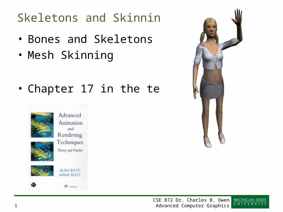
Skeletons and Skinning
• Bones and Skeletons• Mesh Skinning
• Chapter 17 in the textbook.
CSE 872 Dr. Charles B. OwenAdvanced Computer Graphics2
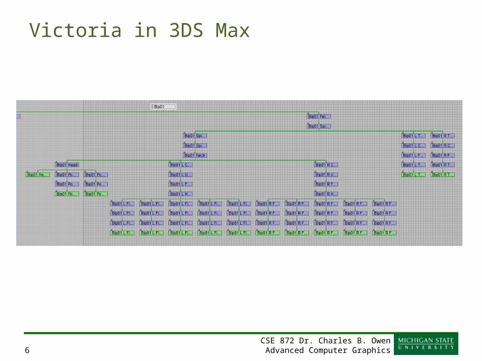
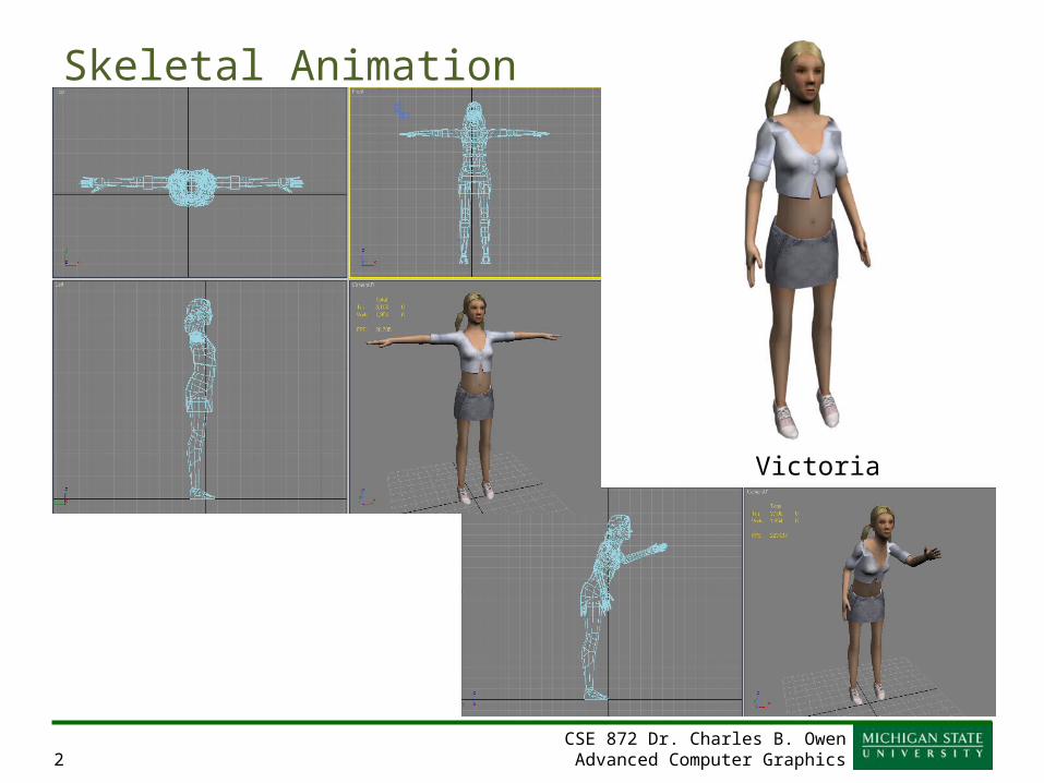
Skeletal Animation
Victoria
CSE 872 Dr. Charles B. OwenAdvanced Computer Graphics3
Skeletons
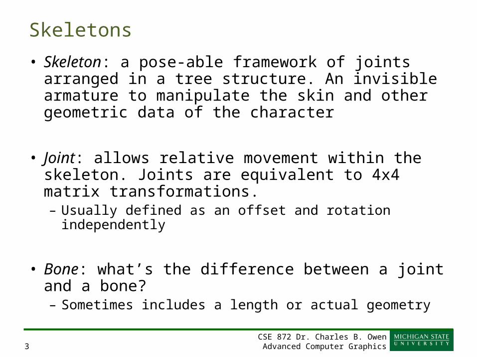
• Skeleton: a pose-able framework of joints arranged in a tree structure. An invisible armature to manipulate the skin and other geometric data of the character
• Joint: allows relative movement within the skeleton. Joints are equivalent to 4x4 matrix transformations. – Usually defined as an offset and rotation independently
• Bone: what’s the difference between a joint and a bone?– Sometimes includes a length or actual geometry
CSE 872 Dr. Charles B. OwenAdvanced Computer Graphics4
DOFs
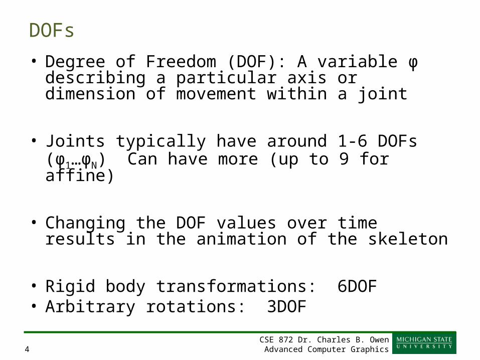
• Degree of Freedom (DOF): A variable φ describing a particular axis or dimension of movement within a joint
• Joints typically have around 1-6 DOFs (φ1…φN) Can have more (up to 9 for affine)
• Changing the DOF values over time results in the animation of the skeleton
• Rigid body transformations: 6DOF• Arbitrary rotations: 3DOF
CSE 872 Dr. Charles B. OwenAdvanced Computer Graphics5
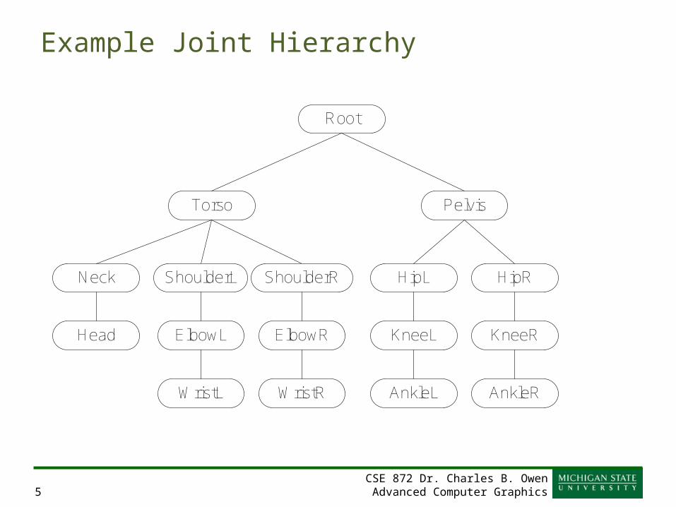
Example Joint Hierarchy
Root
Torso
Neck
Pelvis
HipL HipR
Head ElbowL
WristL
ElbowR
WristR
KneeL
AnkleL
KneeR
AnkleR
ShoulderL ShoulderR
CSE 872 Dr. Charles B. OwenAdvanced Computer Graphics7
Joints
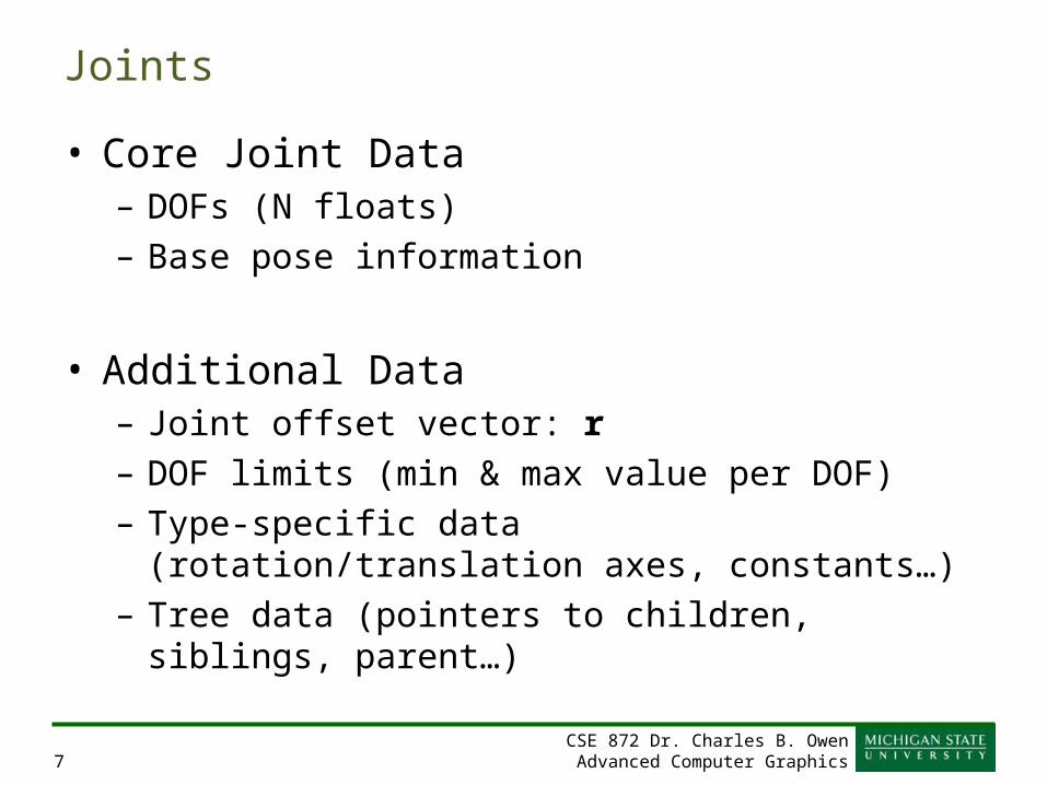
• Core Joint Data– DOFs (N floats)– Base pose information
• Additional Data– Joint offset vector: r– DOF limits (min & max value per DOF)– Type-specific data (rotation/translation axes, constants…)– Tree data (pointers to children, siblings, parent…)
CSE 872 Dr. Charles B. OwenAdvanced Computer Graphics8
Skeleton Posing Process
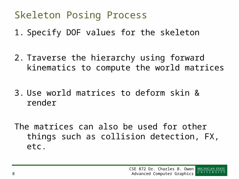
1. Specify DOF values for the skeleton
2. Traverse the hierarchy using forward kinematics to compute the world matrices
3. Use world matrices to deform skin & render
The matrices can also be used for other things such as collision detection, FX, etc.
CSE 872 Dr. Charles B. OwenAdvanced Computer Graphics9
Forward Kinematics
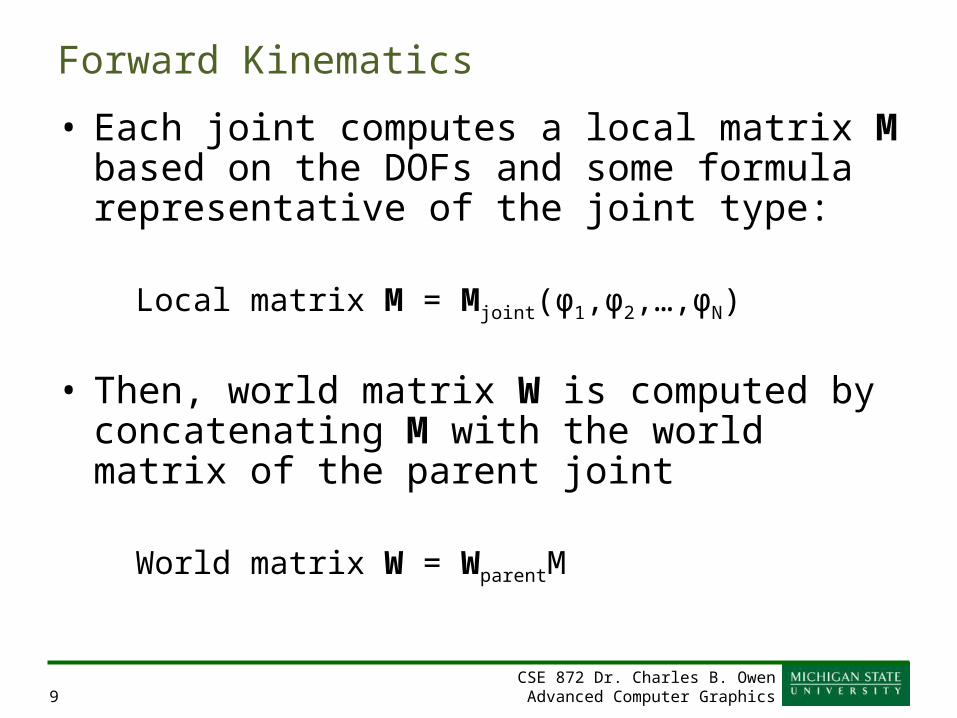
• Each joint computes a local matrix M based on the DOFs and some formula representative of the joint type:
Local matrix M = Mjoint(φ1,φ2,…,φN)
• Then, world matrix W is computed by concatenating M with the world matrix of the parent joint
World matrix W = WparentM
CSE 872 Dr. Charles B. OwenAdvanced Computer Graphics10
Offset Vectors for Joints
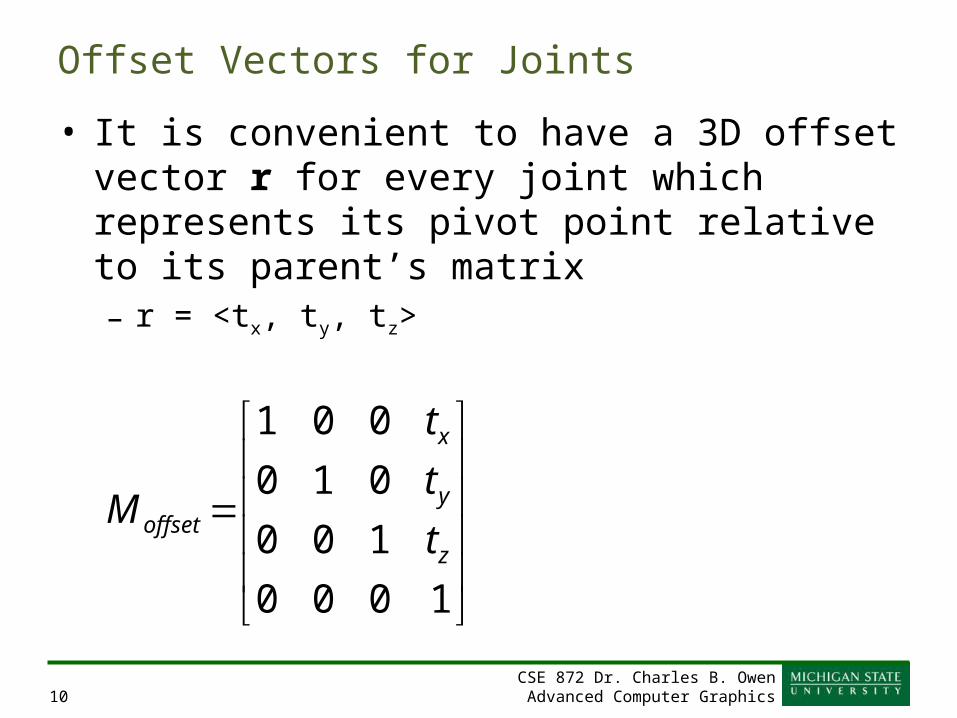
• It is convenient to have a 3D offset vector r for every joint which represents its pivot point relative to its parent’s matrix– r = <tx, ty, tz>
1000
100
010
001
z
y
x
offset t
t
t
M
CSE 872 Dr. Charles B. OwenAdvanced Computer Graphics11
Rotation
• Usually implemented as a Quaternions– Matricies can’t be interpolated easily, Quaternions can…
Ultimately it’s a matrix. We sometimes also have Euler angles. Sometime we have all three.
CSE 872 Dr. Charles B. OwenAdvanced Computer Graphics12
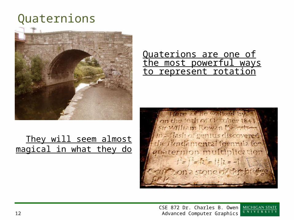
Quaternions
Quaterions are one of the most powerful ways to represent rotation
They will seem almost magical in what they do
CSE 872 Dr. Charles B. OwenAdvanced Computer Graphics13
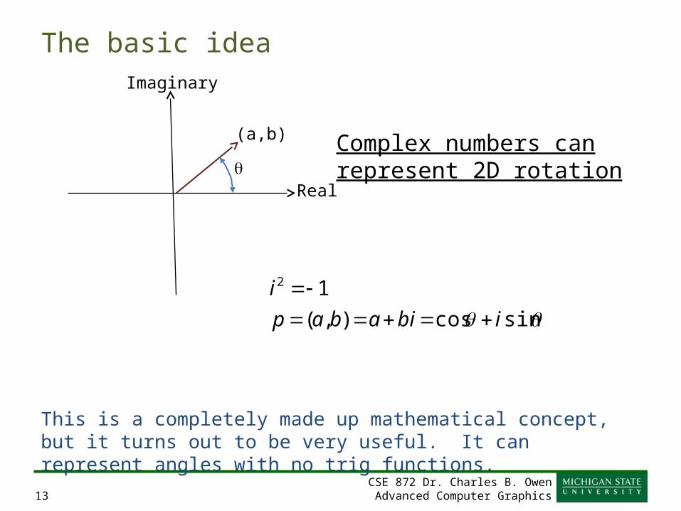
The basic idea
Complex numbers can represent 2D rotation
(a,b)
Real
Imaginary
sincos),(
12
ibiabap
i
This is a completely made up mathematical concept, but it turns out to be very useful. It can represent angles with no trig functions.
CSE 872 Dr. Charles B. OwenAdvanced Computer Graphics14
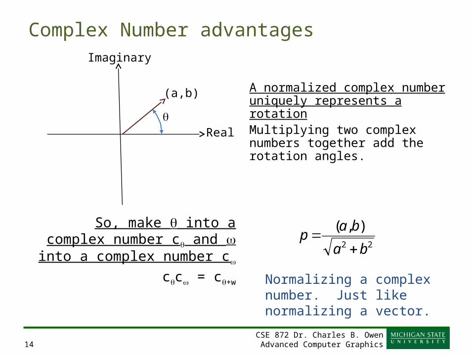
Complex Number advantages
A normalized complex number uniquely represents a rotationMultiplying two complex numbers together add the rotation angles.
So, make into a complex number c and into a complex
number c
cc = c+w
(a,b)
Real
Imaginary
22
),(
ba
bap
Normalizing a complex number. Just like normalizing a vector.
CSE 872 Dr. Charles B. OwenAdvanced Computer Graphics15
Can we extend this to 3D?
Why do we care? Complex numbers represent rotation in a form that can be easily multiplied together with simple multiplication and division operations. We’d love to be able to do that in 3D with something smaller than a matrix. You can compose a rotation and orientation with a single multiplication.
Well, we have real and imaginary. Could we have even more imaginary?
Yes, we can!
William Rowan Hamilton invented quaternions in 1843 which provide a tool for rotation that easily composes and interpolates. We’ll use them a lot.

CSE 872 Dr. Charles B. OwenAdvanced Computer Graphics16
Quaternion Plaque on Broom Bridge in Dublin, Ireland
Here as he walked by on the 16th of October 1843 Sir William Rowan Hamilton in a flash of genius discovered the
fundamental formula for quaternion multiplicationi2=j2=k2=ijk= -1
& cut it on a stone of this bridge
CSE 872 Dr. Charles B. OwenAdvanced Computer Graphics17
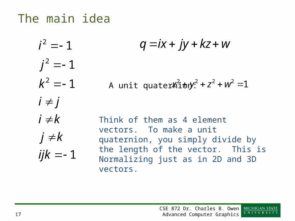
The main idea
1
1
1
1
2
2
2
ijk
kj
ki
ji
k
j
i wkzjyixq
A unit quaternion: 12222 wzyx
Think of them as 4 element vectors. To make a unit quaternion, you simply divide by the length of the vector. This is Normalizing just as in 2D and 3D vectors.
CSE 872 Dr. Charles B. OwenAdvanced Computer Graphics18
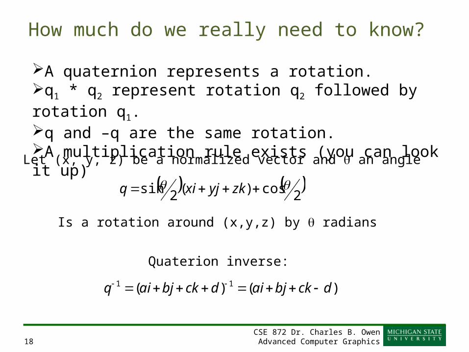
How much do we really need to know?
A quaternion represents a rotation.q1 * q2 represent rotation q2 followed by rotation q1.q and –q are the same rotation.A multiplication rule exists (you can look it up)
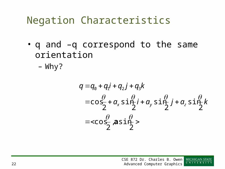
2cos)(2sin zkyjxiq
Let (x, y, z) be a normalized vector and an angle
Is a rotation around (x,y,z) by radians
)()( 11 dckbjaidckbjaiq
Quaterion inverse:
CSE 872 Dr. Charles B. OwenAdvanced Computer Graphics19
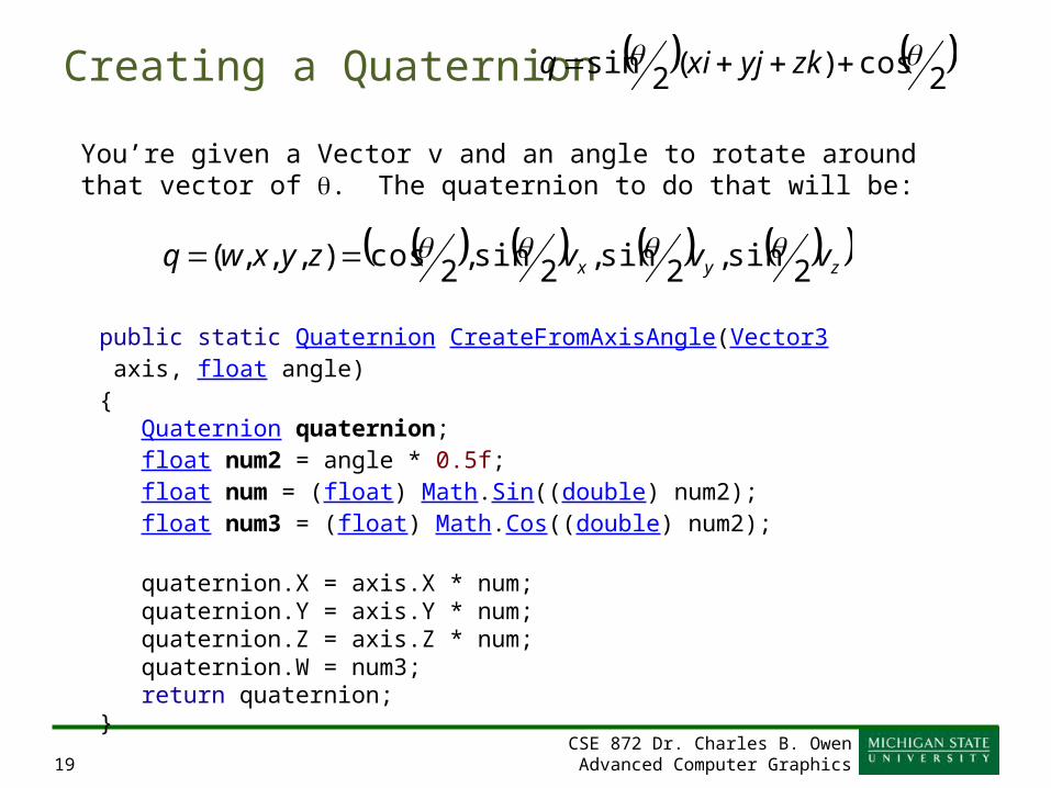
Creating a Quaternion 2cos)(2sin zkyjxiq
You’re given a Vector v and an angle to rotate around that vector of . The quaternion to do that will be:
zyx vvvzyxwq 2sin,2sin,2sin,2cos),,,(
public static Quaternion CreateFromAxisAngle(Vector3 axis, float angle) { Quaternion quaternion; float num2 = angle * 0.5f; float num = (float) Math.Sin((double) num2); float num3 = (float) Math.Cos((double) num2);
quaternion.X = axis.X * num; quaternion.Y = axis.Y * num; quaternion.Z = axis.Z * num; quaternion.W = num3; return quaternion; }
CSE 872 Dr. Charles B. OwenAdvanced Computer Graphics20
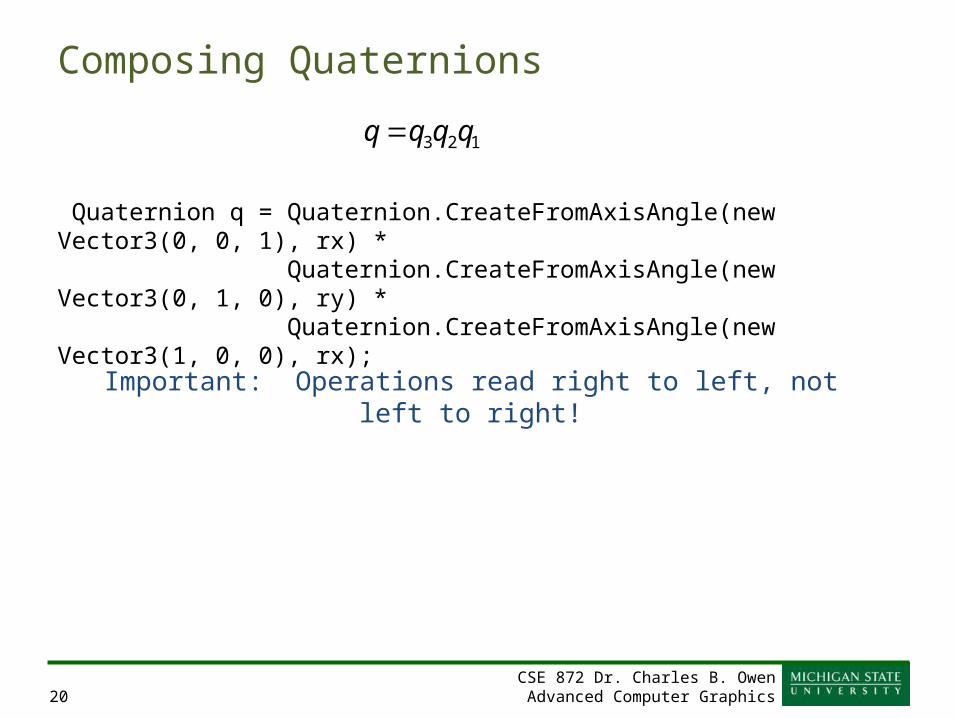
Composing Quaternions
Quaternion q = Quaternion.CreateFromAxisAngle(new Vector3(0, 0, 1), rx) * Quaternion.CreateFromAxisAngle(new Vector3(0, 1, 0), ry) * Quaternion.CreateFromAxisAngle(new Vector3(1, 0, 0), rx);
123 qqqq
Important: Operations read right to left, not left to right!
CSE 872 Dr. Charles B. OwenAdvanced Computer Graphics21
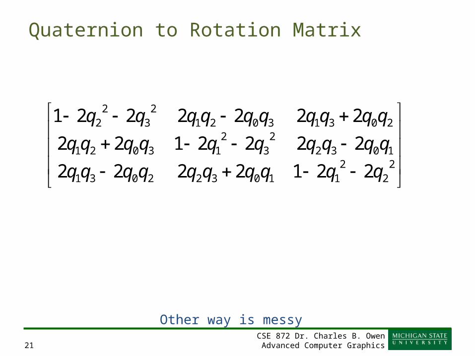
Quaternion to Rotation Matrix
22
2110322031
103223
213021
2031302123
22
2212222
2222122
2222221
qqqqqqqqqq
qqqqqqqqqq
qqqqqqqqqq
Other way is messy
CSE 872 Dr. Charles B. OwenAdvanced Computer Graphics22
Negation Characteristics
• q and –q correspond to the same orientation– Why?
2sin,
2cos
2sin
2sin
2sin
2cos
3210
a
kajaia
kqjqiqqq
zyx
CSE 872 Dr. Charles B. OwenAdvanced Computer Graphics23
Dot Product Characteristic
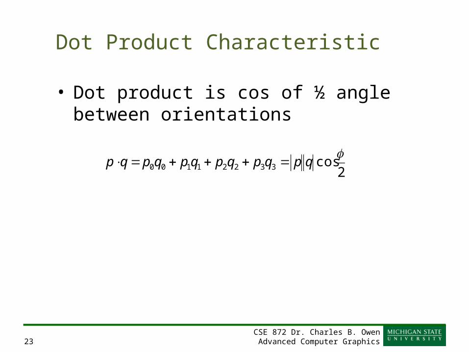
• Dot product is cos of ½ angle between orientations
2cos33221100
qpqpqpqpqpqp
CSE 872 Dr. Charles B. OwenAdvanced Computer Graphics24
Quaterion Interpolation
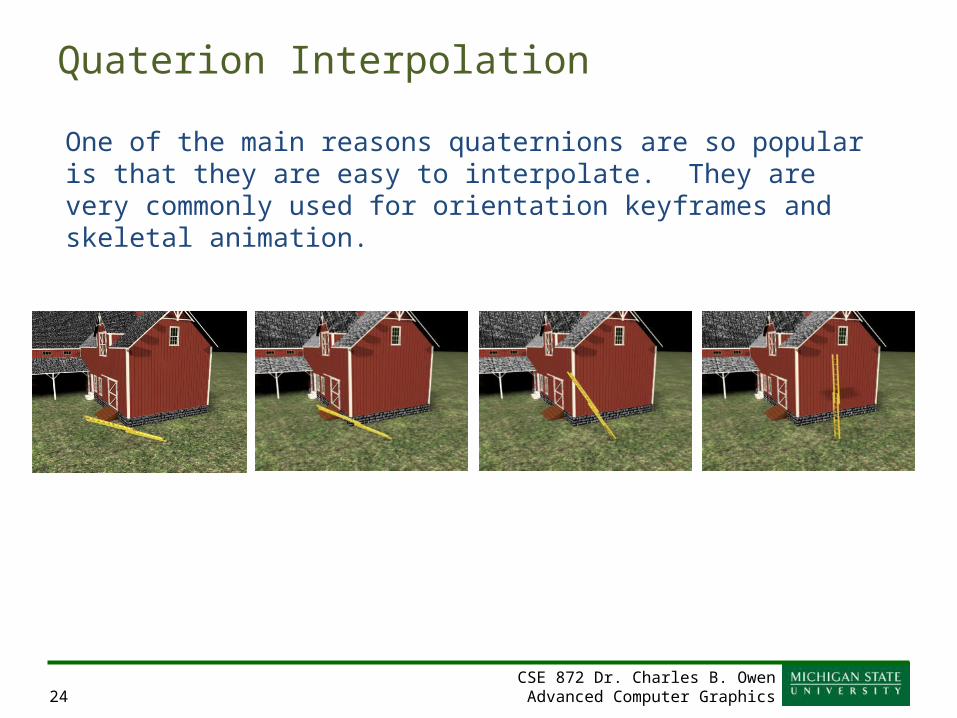
One of the main reasons quaternions are so popular is that they are easy to interpolate. They are very commonly used for orientation keyframes and skeletal animation.
CSE 872 Dr. Charles B. OwenAdvanced Computer Graphics25
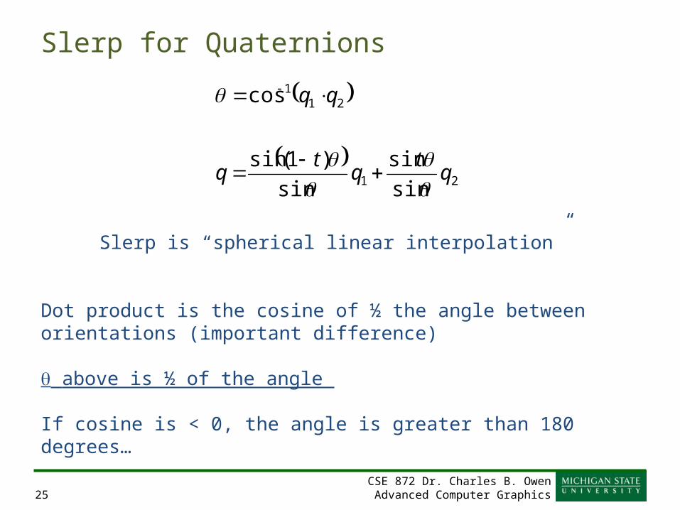
Slerp for Quaternions
21
211
sin
sin
sin
)1(sin
cos
qt
qt
q
Dot product is the cosine of ½ the angle between orientations (important difference)
above is ½ of the angle
If cosine is < 0, the angle is greater than 180 degrees…
Slerp is “spherical linear interpolation”
CSE 872 Dr. Charles B. OwenAdvanced Computer Graphics26
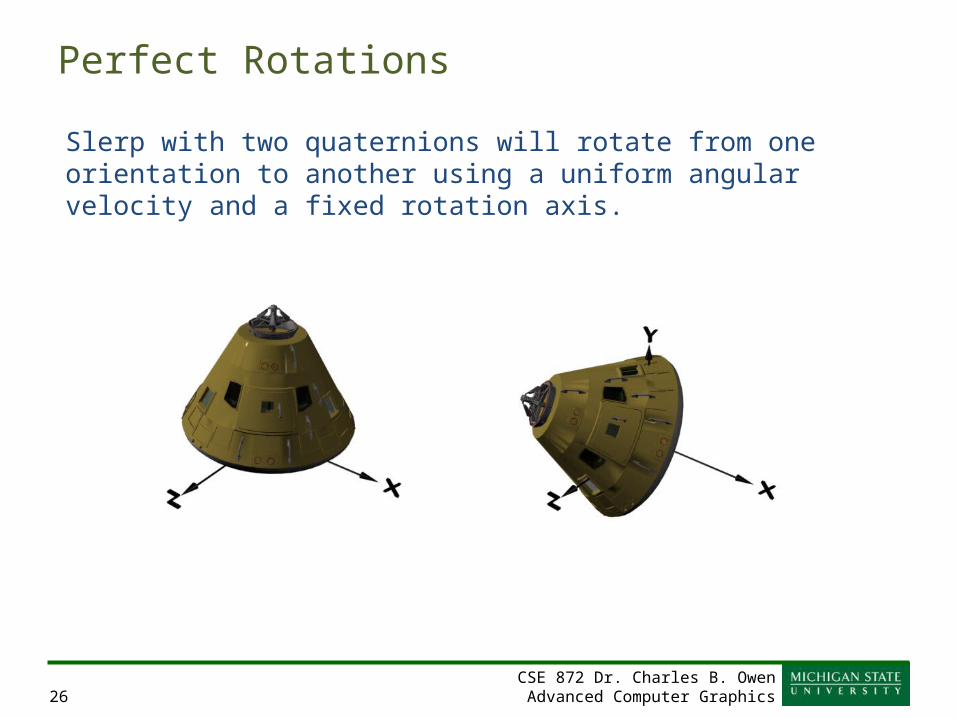
Perfect Rotations
Slerp with two quaternions will rotate from one orientation to another using a uniform angular velocity and a fixed rotation axis.
CSE 872 Dr. Charles B. OwenAdvanced Computer Graphics27
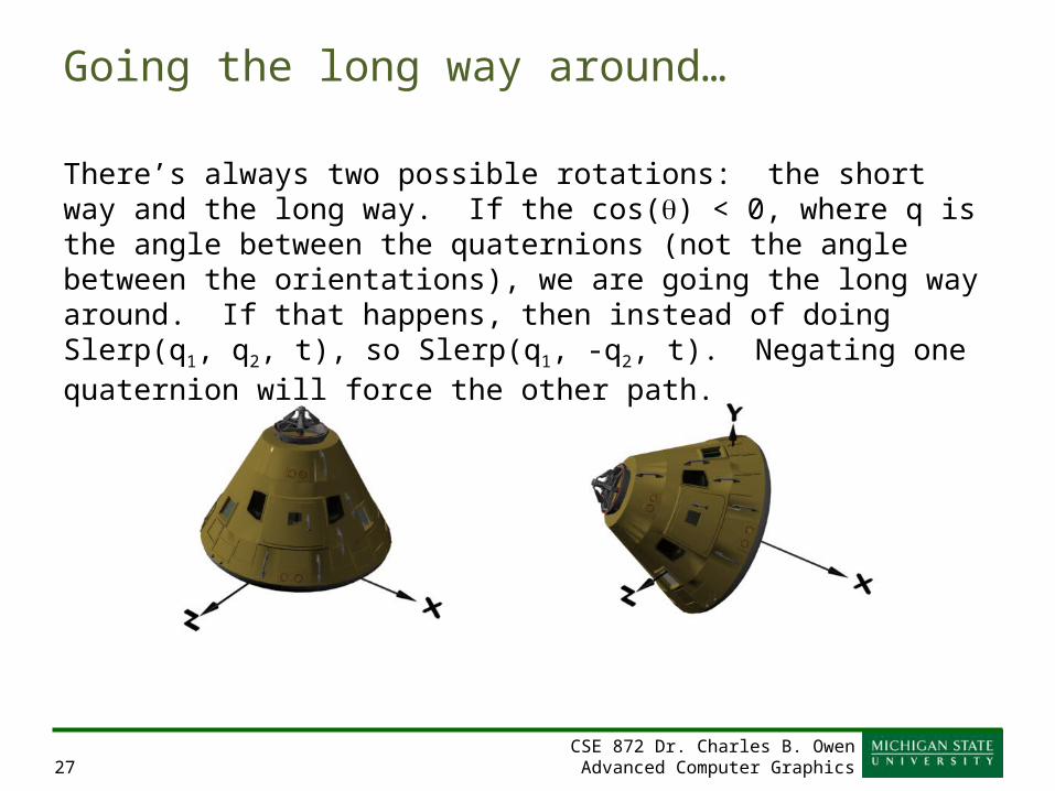
Going the long way around…
There’s always two possible rotations: the short way and the long way. If the cos() < 0, where q is the angle between the quaternions (not the angle between the orientations), we are going the long way around. If that happens, then instead of doing Slerp(q1, q2, t), so Slerp(q1, -q2, t). Negating one quaternion will force the other path.
CSE 872 Dr. Charles B. OwenAdvanced Computer Graphics28
Quaternion Advantages/Disadvantages
AdvantagesCompact notationComposes with simple multiplication
Very efficient and fastInterpolates perfectly with slerp!Perfect for keyframe animation
DisadvantagesNot unique: q and –q are the same rotation and there are other redundancies.4 values to represent 3 things – some redundancy.
CSE 872 Dr. Charles B. OwenAdvanced Computer Graphics29
DOF Limits
• DOF is often range limited– Elbow could be limited from 0º to 150º
CSE 872 Dr. Charles B. OwenAdvanced Computer Graphics30
Skeleton Rigging
• Skeleton Rigging – Setting up the skeleton for a figure– Bones– Joints– DOF’s– Limits
CSE 872 Dr. Charles B. OwenAdvanced Computer Graphics31
Poses
• Adjust DOFs to specify the pose of the skeleton• We can define a pose Φ more formally as a vector of
N numbers that maps to a set of DOFs in the skeleton
Φ = [φ1 φ2 … φN]
CSE 872 Dr. Charles B. OwenAdvanced Computer Graphics32
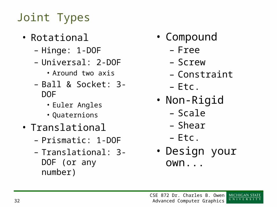
Joint Types
• Rotational– Hinge: 1-DOF– Universal: 2-DOF
• Around two axis
– Ball & Socket: 3-DOF• Euler Angles• Quaternions
• Translational– Prismatic: 1-DOF– Translational: 3-DOF (or
any number)
• Compound– Free– Screw– Constraint– Etc.
• Non-Rigid– Scale– Shear– Etc.
• Design your own...
CSE 872 Dr. Charles B. OwenAdvanced Computer Graphics34
Rigid Parts
• Robots and mechanical creatures – Rigid parts, no smooth skin– Each part is transformed by its joint matrix
• Every vertex of the character’s geometry is transformed by exactly one matrix
where v is defined in joint’s local space
vv M
CSE 872 Dr. Charles B. OwenAdvanced Computer Graphics35
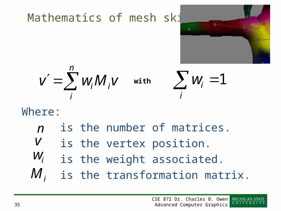
Mathematics of mesh skinning
Where:is the number of matrices.is the vertex position.is the weight associated.is the transformation matrix.
n
iii vMwv
viw
i
iw 1with
iM
n
CSE 872 Dr. Charles B. OwenAdvanced Computer Graphics36
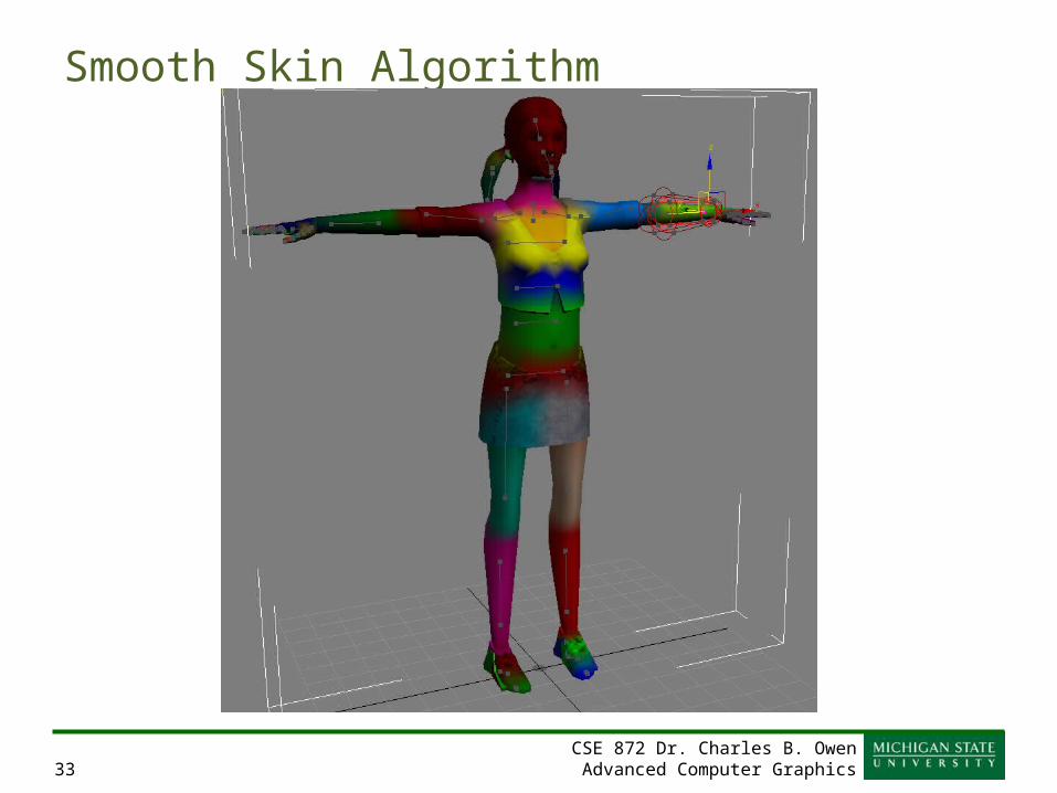
Smooth Skin
• A vertex can be attached to more than one joint/bone with adjustable weights that control how much each joint affects it– Rarely more than 4
• Result is a blending of the n transformations
• Algorithm names– blended skin, skeletal subspace deformation (SSD), multi-
matrix skin, matrix palette skinning…
CSE 872 Dr. Charles B. OwenAdvanced Computer Graphics37
Bone offset method/Vertex offset method• What space should be vertices be in?– If in world coordinates (usually the starting place), M for
each bone must be deformation from original structure– Vertex offset method
• What if vertices defined relative to bones– (which bone?) generally this is not used.– M is now joint manipulation relative to parent– Bone offset method
CSE 872 Dr. Charles B. OwenAdvanced Computer Graphics38
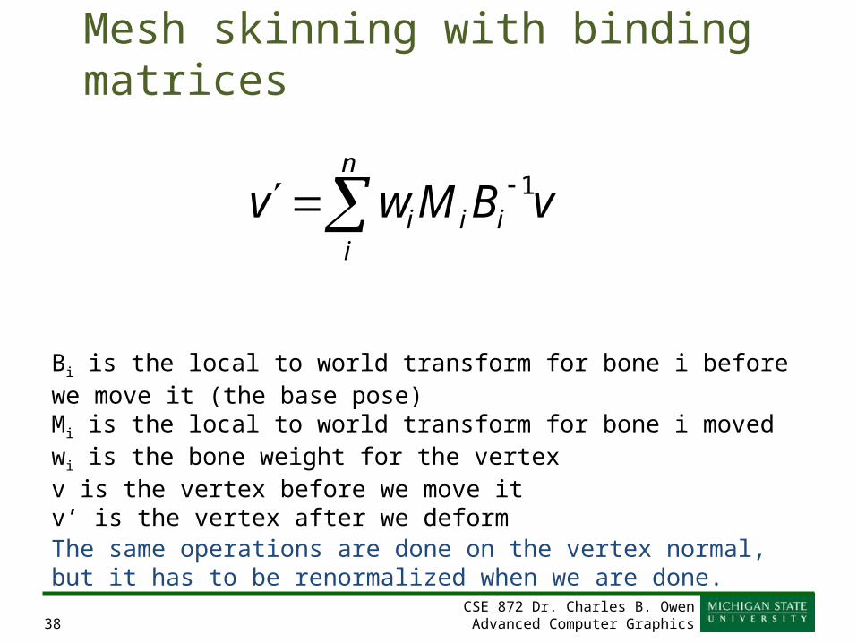
Mesh skinning with binding matrices
n
iiii vBMwv 1
Bi is the local to world transform for bone i before we move it (the base pose)Mi is the local to world transform for bone i movedwi is the bone weight for the vertexv is the vertex before we move itv’ is the vertex after we deformThe same operations are done on the vertex normal, but it has to be renormalized when we are done.
CSE 872 Dr. Charles B. OwenAdvanced Computer Graphics39
Normals
• Normals must also be transformed
• Options– Recompute normals– Do only the rotation of existing normals
• Normals are also blended. But, we MUST renormalize!
CSE 872 Dr. Charles B. OwenAdvanced Computer Graphics40
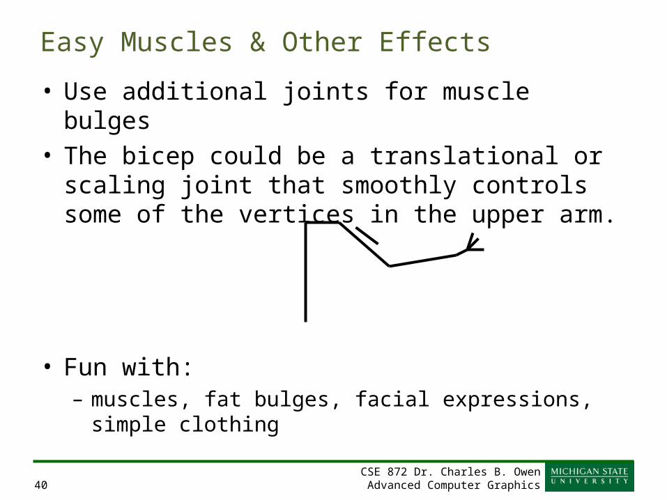
Easy Muscles & Other Effects
• Use additional joints for muscle bulges• The bicep could be a translational or scaling joint that
smoothly controls some of the vertices in the upper arm.
• Fun with:– muscles, fat bulges, facial expressions, simple clothing
CSE 872 Dr. Charles B. OwenAdvanced Computer Graphics41
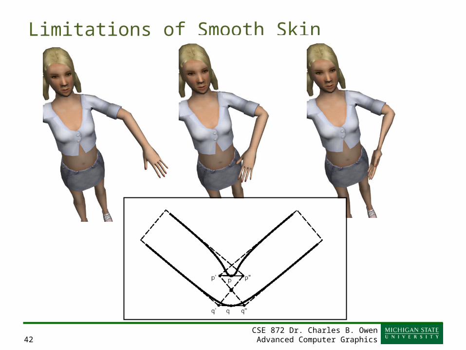
Limitations of Smooth Skin
• Smooth skin is very simple and quite fast, but its quality is limited– Joints tend to collapse as they bend more– Very difficult to get specific control– Unintuitive and difficult to edit
• Still, it is common in games and commercial animation!
• If nothing else, it is a good baseline upon which more complex schemes can be built
CSE 872 Dr. Charles B. OwenAdvanced Computer Graphics42
Limitations of Smooth Skin
CSE 872 Dr. Charles B. OwenAdvanced Computer Graphics43
Bone Links
• Bone links are extra joints inserted in the skeleton to assist with the skinning– Instead of one joint, an elbow may be 2-3 joints– Allows each joint to limit the bend angle!– Why does this help?
CSE 872 Dr. Charles B. OwenAdvanced Computer Graphics44
Shape Interpolation
• An option is to model vertex positions at points in the motion– Interpolate between the positions– More up-front design, but better appearance
• Model an elbow straight and fully bent• Use DOF to determine vertex position, then do the
skinning.
CSE 872 Dr. Charles B. OwenAdvanced Computer Graphics45
Skin Binding
• Skin binding consists of assigning the vertex weights• Binding algorithms typically involve heuristic
approaches
• Any ideas?
CSE 872 Dr. Charles B. OwenAdvanced Computer Graphics47
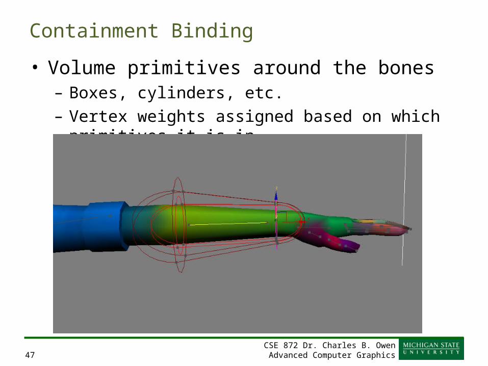
Containment Binding
• Volume primitives around the bones– Boxes, cylinders, etc.– Vertex weights assigned based on which primitives it is in
CSE 872 Dr. Charles B. OwenAdvanced Computer Graphics48
Point-to-Line Mapping
• Which bone is a vertex nearest?• How do we decide to attach to more than one
bone/joint?
CSE 872 Dr. Charles B. OwenAdvanced Computer Graphics49
Delaunay Tetrahedralization
• A tetrahedralization of the volume within the skin• The tetrahedra connect all of the skin verts and joint
pivot points in a ‘Delaunay’ fashion• Basically segments the vertices– How can we get weights?
CSE 872 Dr. Charles B. OwenAdvanced Computer Graphics50
Skin Adjustment
• Mesh Smoothing: Joints attached rigidly, then weights adjusted for smoothness.
• Weight Painting: Indicate weights as colors. • Direct Manipulation: Bend the joint, then drag
vertices where they should be. From this, automatically calculate the weight (least squares estimate).
CSE 872 Dr. Charles B. OwenAdvanced Computer Graphics52
Global Deformations
• A global deformation takes a point in 3D space and outputs a deformed point
v’=F(v)
• A global deformation is essentially a deformation of space• Smooth skinning is a form of global deformation
CSE 872 Dr. Charles B. OwenAdvanced Computer Graphics53
Free-Form Deformations
• Free-form deformations are a class of deformations where a low detail control mesh is used to deform a higher detail skin
CSE 872 Dr. Charles B. OwenAdvanced Computer Graphics54
Lattice FFDs
• The original type of FFD uses a simple regular lattice placed around a region of space
• The lattice is divided up into a regular grid (4x4x4 points for a cubic deformation)
• When the lattice points are then moved, they describe smooth deformation in their vicinity– We are describing moving control points of a curve!
CSE 872 Dr. Charles B. OwenAdvanced Computer Graphics55
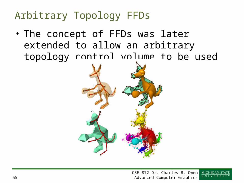
Arbitrary Topology FFDs
• The concept of FFDs was later extended to allow an arbitrary topology control volume to be used
CSE 872 Dr. Charles B. OwenAdvanced Computer Graphics56
Axial Deformations & WIRES
• Another type of deformation allows the user to place lines or curves within a skin– When the lines or curves are moved, they distort the space
around them– Multiple lines & curves can be placed near each other and
interact
• This is like skeletons with curved features– Closer to what muscles really do.
CSE 872 Dr. Charles B. OwenAdvanced Computer Graphics57
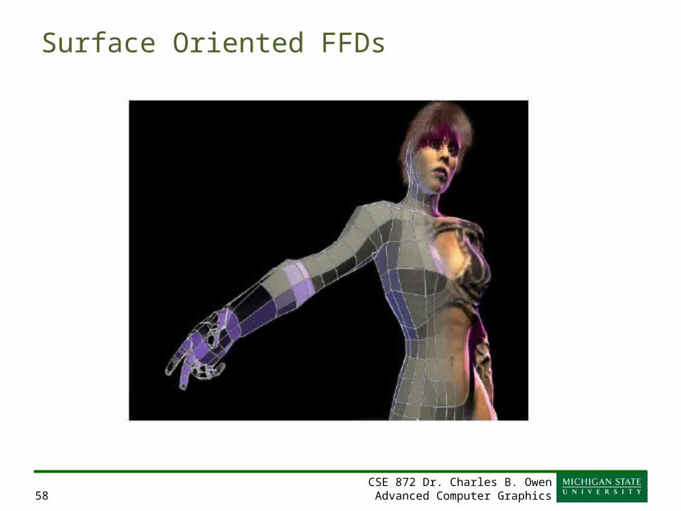
Surface Oriented FFDs
• This modern method allows a low detail polygonal mesh to be built near the high detail skin– Movement of the low detail mesh deforms space nearby
• How is this different from arbitrary topology FFDs?
CSE 872 Dr. Charles B. OwenAdvanced Computer Graphics59
The general idea
• Controlling a small number of low detail vertices is easier than a massive number of skin vertices
CSE 872 Dr. Charles B. OwenAdvanced Computer Graphics60
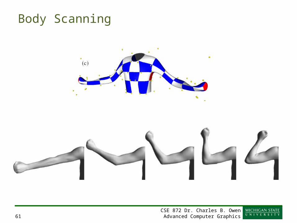
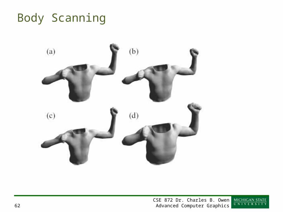
Body Scanning
• Data input for models, deformations• Hardware examples:– Geometry: Laser scanners– Motion: Optical motion capture– Materials: Gonioreflectometer– Faces: Computer vision
CSE 872 Dr. Charles B. OwenAdvanced Computer Graphics64
Anatomical Modeling
• A true anatomical simulation, the tissue beneath the skin must be accounted for
• One can model the bones, muscle, and skin tissue as deformable bodies and then then use physical simulation to compute their motion
• Various approaches exist ranging from simple approximations using basic primitives to detailed anatomical simulations
CSE 872 Dr. Charles B. OwenAdvanced Computer Graphics65
Skin & Muscle Simulation
• Bones are essentially rigid• Muscles occupy almost all of the space between
bone & skin• Although they can change shape, muscles have
essentially constant volume• The rest of the space between the bone & skin is
filled with fat & connective tissues• Skin is connected to fatty tissue and can usually slide
freely over muscle• Skin is anisotropic as wrinkles tend to have specific
orientations
CSE 872 Dr. Charles B. OwenAdvanced Computer Graphics66
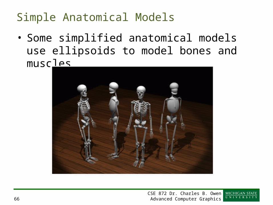
Simple Anatomical Models
• Some simplified anatomical models use ellipsoids to model bones and muscles
CSE 872 Dr. Charles B. OwenAdvanced Computer Graphics67
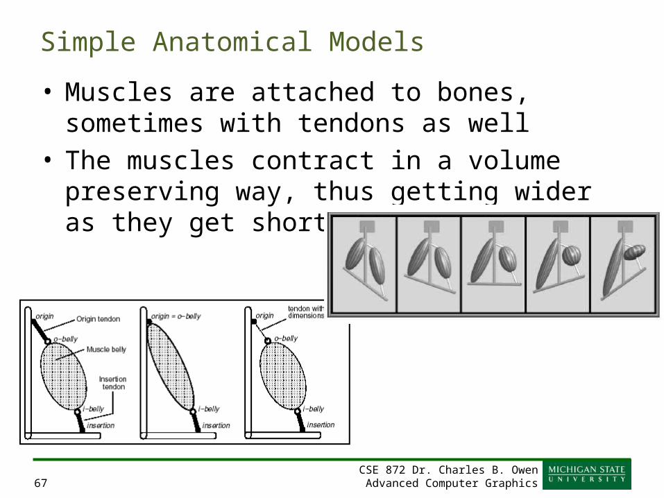
Simple Anatomical Models
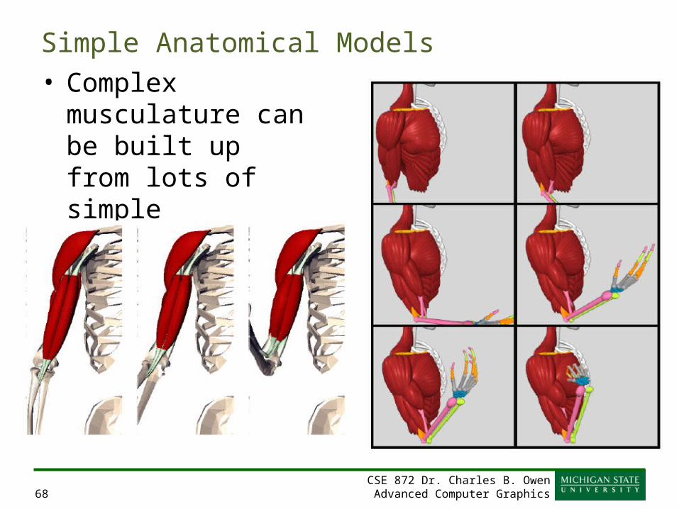
• Muscles are attached to bones, sometimes with tendons as well
• The muscles contract in a volume preserving way, thus getting wider as they get shorter
CSE 872 Dr. Charles B. OwenAdvanced Computer Graphics68
Simple Anatomical Models• Complex musculature
can be built up from lots of simple primitives
CSE 872 Dr. Charles B. OwenAdvanced Computer Graphics69
Simple Anatomical Models
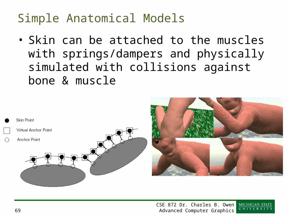
• Skin can be attached to the muscles with springs/dampers and physically simulated with collisions against bone & muscle
CSE 872 Dr. Charles B. OwenAdvanced Computer Graphics70
Detailed Anatomical Models
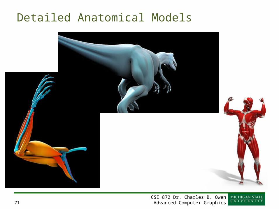
• One can also do detailed simulations that accurately model bone & muscle geometry, as well as physical properties
• This is becoming an increasing popular approach, but requires extensive set up
• Check out cgcharacter.com
CSE 872 Dr. Charles B. OwenAdvanced Computer Graphics71
Detailed Anatomical Models
Top Related