


Languages
Pages
Legal


DP2017-26
Roles of Agricultural Transformation in Achieving Sustainable
Development Goals on Poverty, Hunger, Productivity, and Inequality*
Katsushi S. IMAI
October 12, 2017
* The Discussion Papers are a series of research papers in their draft form, circulated to encourage discussion and comment. Citation and use of such a paper should take account of its provisional character. In some cases, a written consent of the author may be required.

1
Roles of Agricultural Transformation in Achieving Sustainable
Development Goals on Poverty, Hunger, Productivity, and Inequality
Katsushi S. Imai *
Department of Economics, The University of Manchester, UK & RIEB, Kobe University,
Japan
This Version: 11th
October 2017
Abstract
This paper examines the role of the transformation of the rural agricultural sector in achieving
Sustainable Development Goals (SDGs) 1, 2 and 10 drawing upon the cross-country panel data over
the past four decades for 105 developing countries. We define agricultural transformation by three
different indices, namely, (i) the agricultural openness index – the share of agricultural export in
agricultural value added of the country, (ii) the commercialization index - the share of processed
agricultural products, fruits, green vegetables, and meats in all primary and processed agricultural
products, and (iii) the product diversification index to capture the extent to which the country
diversify the agricultural production. Drawing upon the dynamic panel model, we have found that
transformation of the agricultural sector in terms of agricultural openness has dynamically increased
the overall agricultural productivity and its growth and has consequently reduced national, rural and
urban poverty significantly. We have also found that agricultural openness tends to significantly
alleviate child malnutrition, namely underweight and stunting, and improve food security in terms of
energy supply adequacy, protein supply, lack of food deficit and reduction of the prevalence of
anaemia among pregnant women. The agricultural openness is found to be negatively associated with
the Gini coefficient at both national and subnational levels (for both rural and urban areas). Except for
Latin America, product diversification reduces agricultural productivity, implying the efficiency gains
from economies of scale of fewer crops. On the other hand, we argue that the commercialisation does
not generally increase the agricultural productivity and this may be related to a positive effect of the
higher share of cereal production on productivity observed in Sub-Saharan Africa and Latin America.
It has been suggested that policies improving the efficiency of agricultural production, for example
through better rural infrastructure, or promoting agricultural exports, through regional economic
integrations or reducing transaction costs such as tariff and non-tariff barriers, would help to achieve
SDGs 1, 2 and 10 indirectly through the productivity improvement. However, a separate policy to
support the poorest below the US$1.90 a day poverty line is also necessary for achieving SDG 1.
Corresponding Author:
Department of Economics, University of Manchester,
Arthur Lewis Building, Oxford Road,
Manchester M13 9PL, UK
Email: [email protected]
Acknowledgements This study is funded by Strategy and Knowledge Department, IFAD (International Fund for
Agricultural Development). The author is grateful to Paul Winter, Rui Benfica, Fabrizio Bresciani,
Tisorn Songsermsa, Kashi Kafle, Pierre Marion, Neh Paliwal and participants in the research seminar
at Strategy and Knowledge Department (SKD), IFAD, on 5th September 2017, for valuable comments
The author acknowledges useful advice from Raghav Gaiha and Fabrizio Bresciani who contributed
to an earleir draft on Asia and the Pacific which this study builds on. SKD, IFAD, has kindly
provided the data on rural and urban poverty. The opinions expressed in this publication are those of
the author and do not represent those of IFAD.

2
Roles of Agricultural Transformation in Achieving Sustainable
Development Goals on Poverty, Hunger, Productivity, and Inequality
I. Introduction
While many of the middle and low-income countries across the world are still dependent on
the agricultural sector in raising income and producing employment, the nature of agriculture
has dramatically changed over the last four or five decades. In particular, the agricultural
sector has experienced structural transformation, which has been induced by globalisation,
industrialisation, and urbanisation. Despite economic growth, a large section of people in
rural areas still suffers from abject poverty and malnutrition, implying that overall economic
growth has bypassed many.
The growth-inequality relationship is intricately associated with the relationship between
structural transformation and inequality. If labour productivity in rural areas rises at a slower
rate than in urban areas, the disparity between rural and urban areas will widen. Rural-to-
urban migration, however, could have an offsetting effect if migration is temporary and
benefits more rural households than before during the urbanisation process. While many of
the rural regions have benefited from more integrated wholesale and retailing networks and
supply chains (e.g. expansion of supermarket chains to rural areas, horticulture or contract
farming with multinational firms, agricultural production and sales more integrated with
urban regions and developed world, and diversification of rural non-farm sector), whether it
decreases inequality or not is unclear and depends on geographical distributions of these
networks. If structural transformation increases overall productivity and outputs in rural
areas, the structural transformation could reduce income inequality at national levels.
However, if backward regions (e.g. mountainous areas) are left out of the structural
transformation, it is likely to increase inequality. It is thus important to understand better
whether inequality has increased as the country experienced structural transformation in rural
areas.

3
Of particular importance in this context are farm and non-farm linkages and whether
higher rural incomes are in part due to more diversified livelihoods and the emergence of
high-value chains and the extent to which these have reduced rural-urban disparities and
dampened migration. Apart from easier access to credit in order to strengthen farm/non-farm
linkages, and smallholder participation in high-value chains, other major policy concerns
relate to whether remittances could be allocated to more productive uses in rural areas,1
through higher risk-weighted returns-specifically, and whether returns could be enhanced in
agriculture and rural non-farm activities while risks are reduced (Imai, Malaeb, and
Bresciani, 2016).
While a large body of the literature has confirmed that agricultural growth or
development leads to poverty reduction (e.g. Christiaensen et al., 2011; Thirtle et al. 2003; de
Janvry and Sadoulet, 2009), to our knowledge, there have been no work that has
quantitatively analysed the effects of agricultural transformation on poverty. A main
objective of this study is to fill this gap in the literature and examine in detail the role of
transformation of rural agricultural sector in achieving Sustainable Development Goal (SDG)
1 (poverty eradication), 2 (reduction of hunger and malnutrition and doubling agricultural
productivity) and 10 (reduction of inequality) drawing upon the cross-country panel data
over the past four decades for 105 developing countries. Methodologically, using the
dynamic panel model, we will take account of the dynamic transmission of agricultural
transformation to agricultural productivity – defined as log agricultural value added per
worker and its growth as a broad measure of agricultural productivity as well as agricultural
TFP growth (Fuglie, 2012, 2015). In this model, the agricultural transformation is treated as
an endogenous variable by using the dynamic panel model to derive a useful insight into the
1 The literature suggests that access to remittances will improve productivity and reduce poverty only
if they reach the poor and it is used for productive purposes (acquisition of land or machinery) (e.g.
Chiodi et al. 2012; Baldé, 2011).

4
causal relationships among key variables. Finally, we will apply the FE-IV model to take
account of the effects of agricultural transformation on SDGs 1, 2 and 10 via improvement in
agricultural productivity.
To summarise the key findings, we have confirmed that transformation of the agricultural
sector in terms of agricultural openness has dynamically increased the overall agricultural
productivity and its growth and has consequently alleviated poverty, improved malnutrition
and food security, and reduced inequality. Except for Latin America, product diversification
is found to reduce agricultural productivity, implying the efficiency gains from economies of
scale of fewer crops. We have also found that the commercialisation does not generally
increase the agricultural productivity and have suggested that this may be related to a
positive effect of the higher share of cereal production on productivity observed in Sub-
Saharan Africa and Latin America.
Findings are deemed reasonable as we have applied a dynamic panel based on a system
GMM (Generalized Method of Moments) whereby a causal relationship between key
variables (e.g. the causality running from agricultural openness to agricultural productivity)
can be identified under some assumptions. Our findings will provide a number of policy
implications. For example, we will identify the statistically significant correlation between
agricultural openness and agricultural productivity, the latter of which is negatively
associated with some variables that proxy SDGs 1, 2 and 10. A policy implication can be
derived on the role of agricultural openness in achieving SDGs through the improvement in
agricultural productivity – that is, it is important for policymakers to help promote
agricultural exports through regional economic integrations or reducing transaction costs
such as tariff and non-tariff barriers.
The rest of this chapter is organised as follows. After reviewing the concepts of
agricultural transformation in Section II, we will provide three different measures of

5
agricultural transformation we will use in this study in Section III. Section III also discusses
our proxies for SDGs and summarises the data. Section IV then outlines empirical models to
capture the effects of agricultural transformation on SDGs 1, 2 and 10. Section V reports and
discusses the results of the models specified in Section IV. The final section provides
concluding observations with policy implications.
II. Concepts of rural or agricultural transformation
While ‘rural transformation’ (RT) is a broader concept than ‘agricultural transformation’ (AT)
as the former includes the transformation of non-agricultural sector, we will primarily focus
on the structural transformation of the agricultural sector (AT). Conceptually, we draw and
build upon Dawe (2015). While Dawe discusses in detail transformation of the agricultural
sector of middle-income Asian countries, he does not provide a clear definition of
‘agricultural transformation’. Citing Reardon and Timmer (2014), Dawe first discusses ‘the
structural transformation of economies’ and then argues that AT is one of the five key
transitions as a result of sustained income, that is, (i) urbanization, (ii) growth of the rural
non-farm economy, (iii) dietary diversification, (iv) a revolution in supply chains and
retailing; and (v) transformation of the agricultural sector. Consistent with the last transition,
he argues that ‘(t)here are at least three key changes that might be expected to occur during
the agricultural transition: mechanization, increases in farm size, and crop/product
diversification’ (Dawe, p.13, emphasis added). Dawe then reviews some statistical evidence
to show how mechanization took place, farm size increased, and crop diversification took
place in middle-income Asian countries, China, Indonesia, Malaysia, the Philippines,
Thailand, and Vietnam. However, as Dawe did not define AT clearly, it is not clear what sort
of transformation is envisaged. For instance, farm size did not increase uniquely in different
areas of these countries (Figures 14-15 on pp.20-21 in Dawe), but it is not evident whether

6
this heterogeneity implies that AT took place in some parts of the country and did not in other
parts. It is not clear either whether crop/product diversification took place consistently across
these countries (e.g. Malaysia became more specialised in oil crops).
As the term suggests, ‘Transformation’ should imply a fundamental change of the form of
agriculture, rather than a simple change in production or surrounding environment or
economy, which was not fully discussed by Dawe (2015). Barrett et al. (2017) focuses more
on the efficiency of the agricultural sector from a broader perspective. They view the
transformation essentially as the process whereby the agriculture becomes more efficient and
productive. On the other hand, , Ba et al. (1999, p.1) defined AT as a process in which (1)
agriculture becomes increasingly reliant on input and output markets, (2) it integrates more
fully with other sectors of the economy, and (3) local producers in the food system
increasingly incorporate modern scientific knowledge into their practices. The first and the
second aspects imply a greater exposure of the agricultural sector not only to the non-
agricultural sector of the country but also to the rest of the world.
In this paper, following the literature, we define AT as fundamental changes in
agricultural production leading to more efficient production which involves (i) changing
cropping patterns with declining shares of grains and rising shares of non-grains, in
particular, fruits, vegetables, dairy products, and meat, and (ii) a greater exposure to the
agricultural sector and smallholders to the rest of the world, in particular, export markets.
III. Data
Following the discussions on Agricultural Transformation (AT) in the last section, this
section will first provide our three measurements of AT. It will then discuss our measurement
of SDGs. Finally, we will describe the data and the other variables used in our empirical
analyses.

7
(1) Measurement of Agricultural Transformation
While AT encompasses various aspects and can be defined in different ways, given the data
constraints, we will use the following three measures, namely, the commercialization index
or the non-cereal share, agricultural openness and product diversification to capture salient
features of AT following our definition of AT we provided in the previous section.
Commercialization Index or Non-Cereal Share
We use the FAOSTAT data to construct our commercialization index. The index is defined
as the share of processed agricultural products, green vegetables, fruits and meat in the total
agricultural products, including processed and primary products. A precise definition is given
in Appendix 1. The main idea behind this index is that the crops or livestock that has been
processed are more likely to be commercialised than primary crops or livestock2 and that
fruits and green vegetables are likely to be commercialised irrespective of the degree of
processing. On the former, we assume, for instance, that farmers producing maize oil are
more commercialised than those producing maize. While this will be a reasonable
assumption, it is noted that our measure captures only a part of the processed agricultural
products. For instance, we do not have the data of processed cereals (e.g. corn flakes). The
index thus reflects the overall structure of agricultural production in terms of whether the
agricultural crops or livestock are sold as raw crops or processed crops. To overcome the
limitation, we include green vegetables, fruits and meat in the numerator given the fact these
products can be commercialised easily without undergoing on-site processing.
To check the performance of the commercialisation index, we have examined the
relationship between the commercialisation index and the index of mechanisation. Given that
only crude measures are available from FAOSTAT, we have used the number of tractors per
2 The definition of processed agricultural products follows FAO (2011, 2014). Lists of processed and
primary crops or livestock products are given in Appendix 1.

8
Land Area of 100km2. These variables are positively and significantly correlated with an
overall correlation coefficient 0.19 for all developing areas. We have found that a positive
association is the strongest for Asia where the coefficient of correlation is 0.42. A similar
positive relationship between the two variables is found in both Latin America and Sub-
Saharan Africa with the coefficient of correlation 0.30 and 0.18 respectively. As we will see
later, in our cross-country panel estimations for all developing areas, the commercialisation
does not have a statistically significant positive effect on agricultural productivity. To
supplement this, we will construct the variable called ‘Non Cereal share’ (or Cereal Share),
that is, the share of non-cereal product production in total agricultural value added. These
two measures reflect the first dimension of our definition of AT, ‘changing cropping patterns
with declining shares of grains and rising shares of non-grains’.
Agricultural Openness
Agricultural openness is defined as the share of the aggregate agricultural export in the
agricultural value added. Agricultural export is based on the trade file of FAOSTAT
(http://www.fao.org/faostat/en/#data/TP) (in the international US$ (PPP) in 2004-2006). The
agricultural exports include food and non-food agricultural product or exports. Here we do
not include agricultural import because the import of agricultural crops, while influenced by
globalisation and would influence agricultural production systems to some extent, would be
mainly demand-driven and does not reflect the transformation of the agricultural production
systems.3 On the contrary, the higher share of agricultural export tends to reflect more
integration of agricultural production into the rest of the world and is deemed a more suitable
proxy for the agricultural transformation. The agricultural value added is based on World
3 We could construct the share of the input import in the input consumption, but the data on the
fertilizer and pesticides import are available only after 2002 from FAOSTAT and unsuitable for the
present purpose.

9
Development Indicator (WDI) in 2017. As the agricultural sector of the country gets
structurally transformed (e.g. through mechanisation or contract farming), the relative
competitiveness of the agricultural product improves and the agricultural openness index
tends to be higher. We have examined the relationship between the agricultural openness
index and the commercialisation index for all developing areas and for sub-regions. These
two indices, as expected, are positively correlated with the coefficient of correlation 0.34 for
all developing areas. This measure directly captures the second dimension in our definition
of AT.
Product Diversification
We also use the diversity index at the country level drawing upon Remans et al. (2014) who
used an index called ‘Shannon Entropy diversity metric’ to capture the product
diversification at the country level using FAOSTAT. The index can be defined as:
𝐻′ = − ∑ 𝑝𝑖𝑅𝑖=1 ln 𝑝𝑖
where 𝑅 is the number of agricultural products and 𝑝𝑖 is the share of production for the item
𝑖, available from FAOSTAT. The production share, 𝑝𝑖, is defined in terms of the monetary
value at a local price for each product, 𝑖. If the country produces more agricultural products,
including processed and unprocessed crops and the monetary values of products are more
evenly divided among different items, the diversity index, 𝐻′, takes a larger value. On the
contrary, if the country produces a smaller number of agricultural products and the monetary
value of one or two specific products is large, 𝐻′ is smaller. The advantage of using this
index is to simultaneously capture both how equally the country spreads agricultural
production and how many products it produces. A limitation is that it does not take account
of similarities of products in defining the diversity.

10
We have checked whether the product diversification index is positively associated with
the commercialisation index. Contrary to our prediction, commercialisation is not
significantly correlated with product diversification (the correlation coefficient: -0.11). A
negative association is strong in Latin America than in Asia or Sub-Saharan Africa. This
implies that the commercialisation may take place with specialisation, rather than
diversification in some regions (e.g. Latin America). Given that our three measures of
agricultural transformation are not strongly correlated and capture its different dimensions
(see the correlation matrix in Appendix 4), they are inserted as explanatory variables at the
same time.4 We conjecture that the product diversification index partly captures the second
dimension in our definition of AT.
(2) Measurement of SDGs
SDG 1
Our interest lies in examining how agricultural transformation helps the country achieve
SDG 1 (ending poverty in all its forms everywhere), SDG2 (ending hunger, achieve food
security and improved nutrition and promote sustainable agriculture), and SDG 10 (reducing
inequality within and among countries).
On SDG 1, the specific target is set as ‘By 2030, eradicate extreme poverty for all people
everywhere, currently measured as people living on less than $1.25 a day’ (emphasis has
been added by the author) among other goals (e.g. reducing at least by half the proportion of
men, women and children of all ages living in poverty in all its dimensions according to
4 We have plotted product diversification index and the share of non-cereal production in
agricultural value added. As the country movers from the cereal production to non-cereal production,
it sees an improvement in the agricultural productivity. Hence a positive correlation is expected. As
expected, these variables are positively correlated with the coefficient of correlation 0.32, while the
relationship between the two indices is not necessarily clear-cut. We can nevertheless confirm that as
the country produces more non-cereal products the product diversification index tends to be higher. If
we disaggregate it, the correlation for Asia is much higher (0.41) than for Latin America (0.07) or
Sub-Saharan Africa (0.13).
11
national definitions).5 Because it is not possible to use the ‘all its dimensions’ and also
because the World Bank has replaced poverty data at $1.25 a day (2005 PPP) by those at
$1.90 a day (2011 PPP) after the launch of SDGs in 2015, we will use the poverty headcount
ratios at $1.90 and at $3.10 (2011 PPP), while supplementing them with the original
measures for SDG 1, that is, poverty headcount ratios at $1.25 and at $2.00 (2005 PPP). We
further use poverty headcount ratios at $1.25 and at $2.00 for rural and urban areas which
were provided by Strategy and Knowledge Department (SKD), IFAD. A major limitation
about international poverty measures (as well as hunger, food security and inequality
measures) is that the data are highly unbalanced to reflect the years when household surveys
(e.g. Living Standard Measurement Surveys) were conducted in each country. However,
taking the five-year average will mitigate the problem of unbalance in the panel data. It is
also noted that the cross-sectional coverage of poverty data (as well as the data on the Gini
coefficient and child malnutrition) is fairly good (with more than 110 countries).
SDG 2
SDG2 stipulates the goals on food security, malnutrition, and agricultural productivity. For
instance, they include the goals: ‘By 2030, ending hunger and ensure access by all people, in
particular the poor and people in vulnerable situations, including infants, to safe, nutritious
and sufficient food all year round’ (emphasis added by the author), ‘By 2030, ending all
forms of malnutrition, including achieving, by 2025, the internationally agreed targets on
stunting and wasting in children under 5 years of age, and addressing the nutritional needs
of adolescent girls, pregnant and lactating women and older persons’ (emphasis has been
added), and ‘By 2030, double the agricultural productivity and incomes of small-scale food
producers, in particular women, indigenous peoples, family farmers, pastoralists and fishers,
5 See http://www.fao.org/sustainable-development-goals/goals/goal-1/en/ for more details.

12
including through secure and equal access to land, other productive resources and inputs,
knowledge, financial services, markets and opportunities for value addition and non-farm
employment’ (emphasis has been added), among other sub-goals.6 As it is impossible to deal
with all the goals, we will focus on (i) agricultural TFP growth, (ii) malnutrition prevalence
in terms of ‘weight for age’ and ‘height for age’ (% of children under 5), (iii)
the prevalence of undernutrition (FAOSTAT), and (iv) food security indices, namely,
‘Average dietary energy supply adequacy (%)’7. ‘Average protein supply (g/capita/day)’,
‘Depth of the food deficit (kcal/capita/day)’ and ‘Prevalence of anaemia among pregnant
women (%)’. The idea here is that we cover more than one dimension of food security, such
as (i) food availability (dietary energy supply adequacy), (ii) food access (depth of food
deficit), and (iii) utilization (child malnutrition indicators and prevalence of anaemia).
SDG 10
SDG10 is even more diverse than SDGs 1 and 2 and it is not easy to choose the variables for
the empirical analysis. It stipulates the sub-goals as ‘By 2030, progressively achieve and
sustain income growth of the bottom 40 per cent of the population at a rate higher than the
national average’ (emphasis has been added by the author) following the World Bank
arguments in discussion SDGs while the target year, 2015, was approaching (e.g. Dollar et
al., 20168). However, the coverage of the data is not good enough to use it as a main
objective variable. Other sub-goals include: ‘By 2030, empowering and promoting the social,
economic and political inclusion of all, irrespective of age, sex, disability, race, ethnicity,
6 See http://www.fao.org/sustainable-development-goals/goals/goal-2/en/ for more details.
7 It is noted that FAO measures rely mainly on calorie availability, rather than calorie intakes. The
measures are based on the means and variances for a limited number of countries with detailed micro-
data available and a skew normal distribution to determine the proportion of undernourished.
However, for the cross-country analyses, this is the best dataset for food security in terms of coverage
of the countries and thus we have decided to use the FAO measures. See IFAD, WFP, and FAO
(2012) for details of FAO measures on food security. 8 Its discussion paper version was released in 2013.
13
origin, religion or economic or other status.’; ‘Ensuring equal opportunity and reduce
inequalities of outcome, including by eliminating discriminatory laws, policies and practices
and promoting appropriate legislation, policies and action in this regard’, ‘Adopting policies,
especially fiscal, wage and social protection policies, and progressively achieve greater
equality’ among other sub-goals. As these broad goals are rather qualitative or not easy to
quantify by using the historical cross-country data, we will use the Gini coefficient at the
national as well as sub-national levels (i.e. rural and urban areas), while supplementing the
analysis by using income growth of the bottom 40 per cent of the population in a highly
parsimonious specification.
(3) Data and Variables
Our empirical analysis is based mostly on FAOSTAT (http://faostat.fao.org/), World
Development Indicators (WDI) 2015 (http://data.worldbank.org/data-catalog/world-
development-indicators) and the World Bank poverty database (PovCalNet,
http://iresearch.worldbank.org/PovcalNet/). These datasets have been widely used in the
literature and their quality is deemed high, although there are some limitations for specific
variables as we will discuss later. The agricultural total factor productivity (TFP) estimates
are taken from Fuglie (2012 and 2015).9
Table 1 summarizes descriptive statistics of key variables in time-series and cross-
sectional dimensions and their number of observations at regional levels to provide an idea of
the data availability. Appendix 2 lists the names of countries, while further details of the data
and definitions are provided in Appendix 3. We have structured the data as five-year average
panel data to adjust the business cycle of the data following the empirical macro literature.
Most of our variables are based on WDI and FAOSTAT, both of which aggregate micro-
9 There is a limitation in the data of agricultural TFP (Alston and Pardey, 2014) to be discussed later.

14
level household, labour force or industry survey data. As such, it is difficult to quantify the
exact magnitude of measurement errors, it is conjectured that taking the five-year average
will address the errors which occur randomly, while non-random errors (e.g. under-
representativeness of the very poor in the informal sector, or under-reporting of income by
the rich) cannot be addressed. As such, our results on SDGs will have to be interpreted with
caution.
Table 1 Descriptive statistics of key variables in time-series and cross-sectional
dimensions and their number of observations at regional levels
Variable Source Mean
Std. Dev. Min Max Observations
overall Asia
Latin America
SSA
Agriculture value added per worker (first difference) WDI Overall 7.58 1.20 4.94 12.43 776 138 171 288
(constant 2010 US$) between (cross-
section)
1.19 5.38 11.40 113 20 22 41
within (time)
0.29 6.56 8.60 7 7 8 7
Available time periods
1980-2014
Agriculture value added per worker (first difference of log) (constant 2010 US$) WDI Overall 0.10 0.14 -0.44 0.52 663 118 149 247
Between
0.10 -0.11 0.51 112 19 22 41
Within
0.10 -0.41 0.65 6 6 7 6
Available time periods
1985-2014
Agricultural TFP Index growth Fuglie, 2012 Overall 0.01 0.02 -0.14 0.15 1229 228 242 484
Between
0.01 -0.01 0.03 113 21 22 44
Within
0.02 -0.14 0.15 11 11 11 11
Available time periods
1961-2014
Commercialisation Index FAOSTAT Overall 0.68 0.18 0.17 0.99 1265 231 242 462
Between
0.17 0.26 0.99 115 21 22 42
Within
0.04 0.33 0.93 11 11 11 11
Available time periods
1961-2014
Agricultural Openness FAOSTAT Overall 0.36 0.82 0.00 13.17 831 156 197 316
Between
0.69 0.03 5.39 108 19 21 40
Within
0.55 -3.27 8.15 8 8 9 8
1975-2014
Product Diversification FAOSTAT Overall 2.54 0.49 0.27 3.40 1265 231 242 462
Between
0.48 0.53 3.27 115 21 22 42
Within
0.09 2.08 2.83 11 11 11 11
1961-2014
Land Area WDI Overall 758.00 1923 0.46 16400 1410 246 276 516
Between
1927 0.46 16400 118 21 23 43
Within
4.70 702.40 803 11 11 11 11
1961-2014
Population Density WDI Overall 75.4
9 105.3
3 0.78 1245.1
1 1404 246 276 516

15
Between
97.51 1.77 816.21 118 21 23 43
Within
40.04
-342.6
2 504.39 11 11 11 11
1961-2014
Fragility Index WDI Overall 11.2
2 5.88 0.00 23.80 446 78 84 168
Between
5.73 0.25 23.25 113 20 21 42
Within
1.47 6.94 15.45 4 4 4 4
1961-2014
openness WDI overall 70.2
6 36.79 4.30 229.64 1109 193 255 438
between
32.18 19.42 147.10 117 21 23 42
within
18.97 -12.65 173.92 9 9 11 10
1975-2014
Labour force WDI overall 0.73 0.42 0.00 1.00 1428 252 276 528
with secondary between
0.38 0.07 1.00 119 21 23 44
education within
0.18 0.37 1.58 12 12 12 12
1980-2014
povertyhc $3.1 WDI overall 38.6
0 30.79 0.00 98.35 483 100 115 137
between
29.71 0.07 94.53 112 21 23 43
within
9.74 -6.56 75.18 4 5 5 3
1980-2014
povertyhc $1.9 WDI overall 23.0
9 24.30 0.00 94.05 483 100 115 137
between
23.95 0.03 85.57 112 21 23 43
within
8.96 -13.12 62.07 4 5 5 3
1980-2014
Weight for age WDI overall 17.5
6 13.00 0.50 67.30 484 94 117 193
between
11.98 0.60 51.98 111 20 23 44
within
4.78 -2.38 36.99 4 5 5 4
1980-2014
Gini WDI overall 40.8
2 9.18 19.40 74.33 646 125 144 196
between
7.83 25.69 56.31 119 21 23 44
within
4.21 25.24 59.65 5 6 6 4
1980-2014
As we will discuss in details, our main hypotheses are (i) whether agricultural
transformation affects agricultural productivity directly and (ii) whether agricultural
transformation indirectly reduces poverty, inequality or malnutrition indirectly through the
agricultural productivity improvement. As we detailed in the previous section, the
agricultural transformation is proxied by three measures, the commercialization index, the
agricultural openness index and the product diversification index. We will proxy agricultural
productivity by three variables, namely, (i) log of agricultural value added per worker, (ii) the

16
first difference in log of agricultural value added per worker (that is, the growth rate of
agricultural value added per worker) and (iii) the agricultural Total Factor Productivity
(TFP). These are considered broad proxies for agricultural productivity of the country and
deemed an appropriate proxy for one of the sub-goals SDG 2. Our main dependent variable,
log agricultural value added per capita based on WDI has a good coverage of both time-
series and cross-sectional dimensions, covering 7 five-year periods for 113 countries (Table
1). This is considered a broad measure of agricultural productivity in terms of monetary
values of agricultural products to be produced per an agricultural worker. A limitation is that
it is sensitive to sudden demographic changes in rural agricultural sectors, due to migrations.
Agricultural TFP Index growth and our three AT variables, and most of our variables have
few missing observations in both time-series and cross-sectional dimensions, covering at
least 7 five-year periods for more than 100 countries. However, the fragility index covers
only 4 five-year periods and thus we have tried the cases with and without the fragility index.
Appendix 4 reports the correlation among our explanatory variables. In case the fragility
index is included (is excluded) in the model, the maximum correlation coefficient in absolute
value is 0.50 (0.36), which will not cause any concerns for multicollinearity.10
Furthermore, we have compared the values of selected variables in the initial or early five
years (1980-1984 for agricultural transformation or 1990-1994 for SDG variables) and the
last five years to see the overall changes of these variables for both unbalanced and balanced
panel data. Here the early periods are selected so that we have a reasonably large sample to
make meaningful comparisons. The results are reported in Appendix 5. We have found that
(i) both agricultural value added per worker and agricultural TFP significantly increased on
average over the years (for both balanced and unbalanced panel), (ii) on AT variables
10
This is supported by the maximum variance inflation factor of 1.76 (less than 10, the threshold
commonly used in the literature) in the static case.

17
agricultural openness and non-serial share significantly increased on average, while the
commercialization index and the product diversification remain broadly unchanged, and (iii)
all the SDG variables – except poverty at US$1.9 a day (for the unbalanced panel), weight
for age (for the balanced panel) and the Gini coefficient (for both) - significantly improved
over time. This simple comparison is based on unconditional averages of the variables and
ignores their dynamic changes or conditional factors and thus detailed investigations based
on econometric estimations will be carried out in Section V.
Other Covariates
The degree of fragility is captured by ‘fragility index’ proxied by CPIA rating of
macroeconomic management and coping with fragility (1=low to 6=high). The high value
implies low fragility and the low-value high fragility. We have also tried conflict indices, but
prefer the ‘fragility index’ as the former does not cover many countries. We have used the
annual growth rates of agricultural value added per worker based on Imai, Cheng, and Gaiha,
(2017), drawing upon WDI.
We will use the unbalanced panel data for 105 developing countries (or its subset
depending on the choice of explanatory variables) covering East/South East Asia and the
Pacific, South Asia, East Europe and Central Asia, Middle East and North Africa, Sub-
Saharan Africa, and Latin America and Caribbean, with a few robustness checks based on
the balanced panel data. We use the data since 1980 till 2015, but some covariate (e.g.
fragility index) is available in 1990-2010 and so the number of years included in the
regression varies depending on the specification. If the fragility index is dropped, the data
cover nearly four decades. Although the data have some limitations arising from the fact that
many variables from WDI and FAOSTAT were constructed by aggregating the micro-level
data, they are deemed adequate for the objectives of our study.

18
VI. Empirical Models for Agricultural Transformation, Agricultural Growth and
Poverty
The main purpose of our empirical model is to assess the effect of agricultural transformation
(AT) on SDG 1 (poverty), SDG 2 (hunger, food security, and agricultural productivity) and
SDG 10 (inequality). To do so, we will first estimate the effect of AT on agricultural
productivity by treating the former as an endogenous variable. This is important because as
the agricultural productivity improves, the degree of agricultural transformation is also
influenced. We will then estimate the effect of the agricultural productivity on SDGs where
agricultural productivity is estimated by AT in the first stage. Details of estimation strategies
are provided below.
Estimation of Agricultural Productivity with Agricultural Transformation Indices
Given that the commercialisation index primarily influences agricultural productivity, we
will first estimate agricultural value added per worker based on (1) pooled OLS, (2) fixed-
effects (FE) and random-effects (RE) panel model, and (3) the dynamic panel model (or
Blundell-Bond’s (1998) linear dynamic panel model based on a system GMM). While
agricultural transformation, regardless of its definitions (commercialisation index,
agricultural openness, or agricultural product diversification), affects agricultural output or
productivity, the process of agricultural transformation is likely to be accelerated by
agricultural output or productivity. Given that agricultural transformation (AT) is likely to be
endogenous when we estimate agricultural productivity, we apply system GMM by treating
our proxies for AT as endogenous variables by using its own lagged variables in levels and
differences as instruments.11
Model 1: Pooled OLS, FE or RE model for Agricultural Productivity
11
We have also applied the Fixed-Effects IV model by instrumenting AT by external instruments,
namely, urban agglomerations (population in urban agglomerations of more than 1 million (% of
total population)), transport equipment machinery (% of value added in manufacturing), and tariff for
primary goods. The results are broadly consistent with those based on a system GMM.

19
𝑨𝑮𝑖𝑡 = 𝛽0 + 𝑨𝑻𝑖𝑡−1𝛽1 + 𝑿′𝑖𝑡−1𝛽2 + 𝜇𝑖 + 𝜀𝑖𝑡 (1)
For the five-year average panel, t stands for 1 (for 1976-1980), 2 (for 1981-1985), ... , 8 (for
2011-2015) covering the last four decades. i denotes countries (1, 2, ... , 105). 𝑨𝑮𝑖𝑡 is a
dependent variable, an indicator of agricultural productivity. We use either (i) log
agricultural value added per worker, (ii) the first difference of log agricultural value added
per worker or (iii) agricultural TFP growth as a proxy for 𝑨𝑮𝑖𝑡 . We will take the lag of
agricultural transformation indices given that the they are likely to be endogenous and using
its values will partly mitigate the problem of endogeneity, while we will use IV or system
GMM to address the issue more rigorously. Here 𝑨𝑻𝑖𝑡−1 indicates the first lag of a vector of
agricultural transformation, namely, the commercialisation index (or in a few specifications,
the share of cereal or non-cereal products in the total agricultural value added), the
agricultural openness index, and the product diversification index. 𝑿′𝑖𝑡−1 is a vector of
explanatory variables: land area, population density, the fragility index, trade openness, and
labour force with secondary education. 𝜇𝑖 is the country-specific unobservable term, such as,
the institutional capacity or the cultural factor, influencing 𝑨𝑮𝑖𝑡 . 𝜀𝑖𝑡 is an error term,
independent and identically distributed (i.i.d.). This equation is estimated by either pooled
OLS, FE or RE model. We will repeat the same regressions for a subset of the countries,
Asia, Latin America and Caribbean and Sub-Saharan separately to see how the effects of
𝑨𝑻𝑖𝑡−1 are different for different regions.
Model 2: Dynamic Panel Model for Agricultural Productivity
𝑨𝑮𝑖𝑡 = ∑ 𝛼𝑗𝑃𝑗=1 𝑨𝑮𝑖𝑡−𝑗 + ∑ 𝛽𝑘𝑨𝑻𝑖𝑡−𝑘
𝑄𝑘=0 + 𝑿′
𝑖𝑡𝛾 + 𝜂𝑖+𝜀𝑖𝑡 (2)
We will estimate this equation by system GMM (Arellano and Bover, 1995; Blundell and
Bond, 1998) because (i) previous values of 𝑨𝑮 are likely to influence the present value of 𝑨𝑮
due to its persistence and (ii) 𝑨𝑻 is likely to be endogenous. Hence 𝑨𝑻𝑖𝑡−𝑘 is treated as

20
endogenous in the dynamic panel estimation.12
The dynamic panel estimation based on the
system GMM estimator explicitly models the dynamic realisation of agricultural
transformation by having lagged dependent variables.13
As an alternative to the standard first
differencing approach14
, we can use the lagged differences of all explanatory variables as
instruments for the level equation and combine the difference equation and the level equation
in a system. Here the panel estimators use instrumental variables based on previous
realisations of the explanatory variables as the internal instruments, using the Arellano-
Bover and Blundell-Bond System GMM estimator with additional moment conditions. 15
Such a system gives a more consistent estimator under the assumptions that there is no
second order serial correlation and the instruments are uncorrelated with the error terms. As a
robustness check, in one case, we will add an external instrument, namely, a lagged value of
transport equipment machinery, to capture the overall effectiveness and transaction costs in
transporting or exporting goods from rural areas to cities or abroad.
We have repeated all the regressions at the regional levels (namely Asia, Latin America,
and Sub-Saharan Africa). Given a small n and a relatively small sample size in this case, a
finite sample correction has been made for the variance by using the robust estimator when
two-step estimations are feasible (Windmeijer, 2005).
12
Ideally, both directions of causality from 𝑨𝑻𝑖𝑡 to 𝑨𝑮𝒊𝒕 , and from 𝑨𝑮𝒊𝒕 to ∆𝑨𝑻𝑖𝑡 should be
explicitly considered in the model. However, we consider mainly the former (by treating 𝑨𝑻𝑖𝑡 and its
lags endogenous in a system GMM). 13
The inclusion the lags up to the second period is guided by statistical significance of the third lag as
well as specification tests, such as serial correlation tests, AR(1) and AR(2). An inclusion of the third
lag, however, does not change the results significantly, although the number of observations reduces. 14
Two issues have to be resolved in estimating the dynamic panel model. One is endogeneity of the
regressors and the second is the correlation between (𝐴𝐺𝑖𝑡−1 − 𝐴𝐺𝑖𝑡−2) and (𝜀𝑖𝑡−𝜀𝑖𝑡−1) (e.g. see
Baltagi, 2005, Chapter 8). Assuming that 𝜀𝑖𝑡 is not serially correlated and that the regressors in 𝑿𝑖𝑡 are
weakly exogenous, the generalized method-of-moments (GMM) first difference estimator (e.g.
Arellano and Bond, 1991) can be used. 15
See Roodman (2009) for more details of System GMM and practical guides.

21
Model 3: Fixed-Effects IV Model for SDGs (Poverty, Malnutrition, Food Security, and
Inequality)
First Stage:
𝑨𝑮𝑖𝑡 = 𝛽0 + 𝑨𝑻𝑖𝑡−1𝛽1 + 𝑿′𝑖𝑡−1𝛽2 + 𝜇𝑖 + 𝜀𝑖𝑡 (3)
Second Stage:
𝑺𝑫𝑮𝑖𝑡 = 𝛾0 + 𝑨�̂�𝑖𝑡𝛾1 + 𝑿′𝑖𝑡−1𝛾2 + 𝜗𝑖 + 𝜀𝑖𝑡 (4)
Here in order to make the estimation for SDG tractable16
, we will relax the assumption that
𝑨𝑻𝑖𝑡−1 is endogenous in the equation for 𝑨𝑮𝑖𝑡 in Model 2 (system GMM). We assume that,
by taking the lag of 𝑨𝑻, namely agricultural commercialisation index, agricultural openness,
and production diversity, 𝑨𝑻𝑖𝑡−1 is exogenous in Equation (3) and serve as instruments to
identify the first-stage equation. In other words, following Imai, Gaiha, and Bresciani (2016)
we will estimate the effect of 𝑨𝑻 on 𝑺𝑫𝑮 only through increase in production of the
agricultural sector per worker.
Whether 𝑨𝑻𝑖𝑡−1 serves as a valid instrument should be discussed for each goal in SDGs,
i.e., a dependant variable in the second stage. On poverty, while the literature suggests that a
higher agricultural productivity or output leads to poverty reduction, it is unlikely for the
increase in agricultural export, the increase in more processed crops or the increase in kinds
of agricultural crops (keeping the agricultural production constant) to influence national,
urban or rural poverty directly. This is because 𝑨𝑻 is the transformation of the agricultural
sector, leading to increase productivity, but poverty is reduced as a result of changes in
agricultural income/outputs, not as a result of the structural transformation itself. Of course,
even without any change in the agricultural production or productivity, increasing the share
of processed crops or livestock, shifting the domestic sale to export of crops, or introducing
the new types of crops may lead to increase rural non-farm sector jobs and reduce poverty in
16
It is noted that poverty or inequality panel data have more missing variables than the data on
agricultural productivity.

22
the long run. However, in the short run, it is reasonable to assume that 𝑨𝑻 primarily and
directly affects agricultural productivity (𝑨𝑮) and its effect on poverty is realised only
indirectly through the improvement in 𝑨𝑮. The validity of this assumption can be checked by
specification tests. The same reasoning would apply when we estimate other goals in SDGs,
such as rural or urban poverty, child malnutrition, food security indices and inequality. For
instance, the overall food security could increase as a result of an increase in rural non-
agricultural jobs due to the shift of domestic sales of crops to export, but this effect is indirect
and is realised only in the long run.
Alternatively, in a few specifications, we estimate Equations (2) and (4) simultaneously.
That is, in estimating Equation (4), we first derive the predicted value of 𝑨𝑮𝑖𝑡 (𝑨�̂�𝑖𝑡) and
those of the error term 𝜀�̂�𝑡 in Equation (2) and then put them in the fixed effects model where
a variable in SDGs is estimated by those prediction terms and control variables where the
standard errors are adjusted by bootstrapping. This is aimed to overcome the data limitations
where some of the variables on SDGs are available for a limited number of years, while 𝑨𝑮𝑖𝑡
has a better coverage. The prevalence of undernutrition (POU) is estimated by the variables
on agricultural transformation directly by the fixed effects model as 𝑨�̂�𝑖𝑡 is not statistically
significant in the first stage of the FE-IV estimation outlined above.
V. Results
In this section, we will summarise and discuss the results derived for Models 1-3 for the five-
year average panel data.17
(1) Results of Models 1-2: All Developing Areas
17
We have estimated the same models using the annual panel data and have obtained broadly similar
results.

23
Table 2 shows the results on the effect of agricultural transformation indices on the level of
agricultural value added per worker using the five-year average panel. Case 1 and Case 3 of
Table 2 (pooled OLS and RE model) indicate that there is an overall positive and significant
association between the commercialisation index and agricultural productivity (broadly
defined as log agricultural value added per worker). Given that the commercialisation index
is shown as the share (0 to 1) and that the left-hand-side variable is in the log, a 1% increase
in the commercialisation in the previous year/period is associated with the 0.4%-1.4%
increase in agricultural value added per worker. However, it is noted that the pooled OLS
does not take account of the country unobservable effect and the RE model is not favoured
over the FE model as the Hausman test is statistically significant. So we cannot make any
claim on the causality between the two variables.
Table 2 Effects of Agricultural Transformation on the Level of Agricultural Value
Added per capita (Five-Years Average Panel) Dep. Variable log agricultural value added
Regions All Developing Areas
Case 1 Case 2 Case 3 Case 4 Case 5 Case 6 Case 7 Case 8
EXP. VARIABLES Pooled
OLS FE RE SGMM SGMM
SGMM SGMM SGMM
With an
initial value With an
external IV Balanced
panel
log Agricultural Value Added per worker, an initial value
0.0104
[1.523]
Commercialization Index 1.386*** -0.127 0.443* -0.155
-0.364*** -0.263*** 0.124 -0.364*** (-1)
[4.503] [-0.423] [1.647] [-1.101] [-3.225] [-9.636] [1.239] [-3.225]
Agricultural Openness(-1) -0.0121 0.0430** 0.0464** 0.0422*** 0.0491*** 0.0432*** 0.0389*** 0.0491***
[-0.194] [2.185] [2.294] [6.105] [16.55] [5.426] [10.27] [16.55]
Product Diversity(-1) -
0.281*** -0.00207 -0.0998 -0.0181
-0.0627 0.0202* -0.00265 -0.0627
[-2.600] [-0.0141] [-0.821] [-0.283] [-1.222] [1.732] [-0.0402] [-1.222]
Control Variables Yes Yes Yes Yes Yes Yes Yes Yes
Number of lags of dependent variables in the right hand side
0 0 0 2 2 2 2 2
Observations 370 370 370 244 417 417 195 346
R-squared 0.522 0.259
Number of countries 102 102 92 96 96 64 70
AR(1) in first difference (Pr > z )
0.038** 0.001*** 0.038 0.001 0.001
AR(2) in first difference (Pr>z)
0.148 0.08* 0.148 0.08 0.08
Sargan statistic
Over identification tests
Sargan Test (Chi2)
6.03 6.03 28.7 28.7 21.74
Prob > chi2
0.813 0.052 0.052 0.244 0

24
Hansen Test (Chi2)
6.48 6.48 28.78 28.78 19.83
Prob > chi2 0.774 0.051 0.051 0.343 0.078
Breusch and Pagan Lagrangian multiplier test for random effects
chibar2(01) =
435.57***
Prob > chibar2 =
0
Hausman Test (chi2(7)) 29.27
Prob>chi2 = 0.0001
Notes: t-statistics in brackets (*** p<0.01, ** p<0.05, * p<0.1). System GMM is based on the two-step robust estimators. Control variables are Land area, Population Density, Fragility Index, Trade Openness, and Labour Force with Secondary Education. Same control variables will be used in Tables 3-8.
The main conclusion that can be safely derived from Table 2 is that agricultural openness
causes higher agricultural production per worker, a broad measure of agricultural
productivity after taking into account the endogeneity of agricultural openness in Cases 4-8
of Table 2. This is suggested by statistically highly significant coefficient estimates of
agricultural openness in these cases. In case of System GMM (Cases 4-8), a 1% increase in
the agricultural openness leads to an increase in agricultural value added per capita by 0.04-
0.06%.18
The difference is due to the fact that the effect of lagged agricultural production is
included in the latter. We have dropped the fragility index in Cases 6 and 7 of Table 2 and
thus cover nearly four decades, while other cases cover only two decades. However, the sign
and statistical significance of coefficient estimates for 𝑨𝑻 are similar in these cases. We can
conclude that among three proxies for 𝑨𝑻, the agricultural openness is key to promoting
agricultural productivity. On the results of control variables, we observe that, if the country is
more fragile (or vulnerable), the agricultural value added per worker tends to be negatively
affected.
Sensitivity tests are carried out in Cases 6-8 of Table 2. First, to see whether the initial
differences in the agricultural development matters, we have carried a robustness check in
Case 6 where the initial level of agricultural value added per worker (defined as the value in
18 On the results of System GMM in Cases 5-8 in Table 2 are broadly justified by the specification
tests as AR(1) is significant and AR(2) is not at the 5% level, while both Sargan and Hansen tests are
not statistically significant at the 5% level. The case with the initial level of log agricultural value
added per worker (Case 6) is weak as the test statistics are significant at the 10% level for both
Sargan and Hansen tests. As the Hansen test is deemed more robust than the Sargan test, we will
mainly adopt the former in evaluating the performance of the dynamic model.

25
the earliest period during the first three periods in the case where the five-year average panel
is used, or the value in the earliest year during the first 15 years for the annual panel). The
initial level of agricultural development is positive and not statistically significant. This
implies that the country which had already developed in agricultural productivity in early
years tends to keep the high levels of agricultural productivity in later years. It is noted that
an overall pattern of the results remains same, though the commercialisation index turns
negative. In Case 7 we have used not only internal instruments but also an external
instrument, that is, a lagged value of transport machinery. In Case 8 we have dropped the 26
countries with missing observations (71 observations) in Case 5 to make the panel balanced.
The result does not change substantially.19
In Cases 5, 6, and 8 of Table 2, the commercialisation index has turned out to be negative
and significant, which is somewhat puzzling given that we have hypothesised that
commercialisation is one of the key features of agricultural transformation. One of the
reasons is that, by the construction of the index with a focus on processed crops, fruits and
green vegetables, the commercialisation index is negatively correlated with the share of
cereal crops, which is sometimes important for the higher agricultural production. The
coefficient of correlation based on our five-year panel data is 0.06. Barrett et al. (2017) have
suggested that in Zambia maize and cereal output have doubled (with more than 50%
increase in cereal yield) and poverty remained unchanged during the period between 2006
and 2011, while in Rwanda cereal output tripled and poverty reduced by 12% (45% of which
due to an increase in agricultural productivity and marketing) from 2006 to 2011. So in some
countries, the intensifications of cereal production appear to be key to productivity increase.
19
It is not straightforward to choose whether unbalanced or balanced data are used and this should be
judged with respect to the study objective and the pattern for missing observations (Baltagi and Song,
2006) as making the data balanced may worsen the performance of the estimators when compared to
those from the entire unbalanced data (Baltagi and Chang, 1994). We have decided to use unbalanced
data as covering more countries is crucial for the main objective of our study.

26
In Table 3 we have replaced the commercialisation index by the share of cereal
production based on the five-year average panel and a system GMM (without the fragility
index) for all developing areas, Asia, Latin America, and Sub-Saharan Africa. In Case 1 of
Table 3 for all developing areas, while agricultural openness remains positive and significant,
cereal share is also positive and significant, implying that the higher serial production will
improve the broad measure of agricultural productivity in terms of log agricultural value
added per worker. This is due to the positive effect of crop share in Sub-Saharan Africa and
Latin America (Cases 3 and 4), while it is negative and significant for Asia (Case 2) where
cereal production has become mature and shift to non-cereal production is more important.
In disaggregated cases, agricultural openness is positive and significant only for Latin
America. In all the regional regressions where System GMM is applied, standard errors are
based on the robust estimator for the small sample in regional regressions (Windmeijer,
2005).
Table 3 Effects of Cereal Share on the Level of Agricultural value added per worker
Dep. Variable log agricultural value added
Regions All developing areas
Asia Lain America
SSA All developing areas
Data Five-Years Average Panel
Case 1 Case 2 Case 3 Case 4 Case 5
EXP. VARIABLES SGMM SGMM SGMM SGMM SGMM
Cereal Share (-1) 0.195* -0.225** 0.371** 0.702*** 0.155
[1.684] [-2.650] [2.161] [2.994] [1.272]
Cereal Share (-1)*Land
2.12e-08***
[2.826]
Agricultural Openness (-1) 0.0535*** 0.170 0.0619*** 0.115 0.0539***
[8.506] [1.463] [6.529] [1.348] [8.685]
Production Diversity -0.121 0.0709 -0.663*** 0.138 -0.127*
[-1.629] [1.003] [-7.004] [1.527] [-1.688]
Control Variables Yes Yes Yes Yes Yes Number of lags of dependent variables in the right hand side 2 2 2 2 2
Observations 325 61 80 124 325
Number of country 95 17 21 32 95
AR(1) in first difference (Pr > z ) 0 0.994 0.03 0 0
AR(2) in first difference (Pr>z) 0.118 0.723 0.538 0.087 0.134
Over identification tests

27
Sargan Test (Chi2) 10.04 21.55 7.7 20.33 10.09
Prob > chi2 0.612 0.723 0.808 0.061 0.608
Hansen Test (Chi2) 10.79 10.75 9.05 14.14 10.69
Prob > chi2 0.574 0.55 0.698 0.528 0.556
Notes: t-statistics in brackets (*** p<0.01, ** p<0.05, * p<0.1). Standard errors are based on the robust estimator for the small sample in regional regressions (Windmeijer, 2005).
One of the reasons why the share of cereals is positive for Latin America and Sub-
Saharan Africa, while it is negative for Asia, is that the land abundance determines the extent
to which cereal production contributes to the overall agricultural productivity in the long run,
that is, the country with the relatively small arable land area cannot raise the productivity
without relying on large land. To test this, we have inserted an interaction term of the land
area and the share of lagged cereal production (as well as the cereal share and the land area)
in Case 5. The result shows that the interaction is positive and statistically significant at the
1% level, while the coefficient estimate of the cereal share is positive and non-significant.
This implies that the initial endowment of the country explains the role of cereal (or non-
cereal share) as well as of the commercialisation index in determining the agricultural
productivity.
As an extension we have tried a case where the dependent variable is the growth (rather
than the level) of agricultural value added per worker, that is, the first difference of log of
agricultural value added per worker for the five-year average panel based on the system
GMM. The results are reported in Appendix 6. Consistent with the results in Table 2, if the
share of agricultural export in agricultural value added of the country increases, the
agricultural productivity increases. We can conclude that a 1% (or 10%) increase in the
agricultural export share leads to the productivity growth by 0.04%-0.05% (or 0.4%-0.5%).
On the contrary, the commercialisation index is negatively and significantly associated with
the productivity growth. This implies that only a shift from primary crops to processed crops
or green vegetables/fruits may not lead to the productivity growth because there is a time lag

28
for the new crop productions to get more productive (e.g. due to the initial fixed investment)
or because cereal productions are sometimes more productive than non-serial productions.
We have also tested our earlier hypothesis by inserting the cereal share and the initial level of
log agricultural value added per worker. First, the share of cereal products positively
influences the growth of agricultural productivity. The initial level of log agricultural value
added per worker, on the contrary, is positive and statistically insignificant. Inserting this
term will not change the overall pattern of the coefficient estimates of other variables.20
(2) Results of Model 2: Asia, Latin America, and Sub-Saharan Africa
Given the possible heterogeneity of the effect of agricultural transformation on agricultural
development, we applied the same model for Asia, Latin America and Caribbean, and Sub-
Saharan Africa as presented in Table 6. Given the results in Table 3, we use the non-cereal
share as an alternative to the commercialisation index. We find that in Asia agricultural
openness decreases agricultural TFP growth in Case 3.21
More importantly, the results Cases
1 and 3 confirm that the non-cereal share increases not only log agricultural value added per
capita but also the growth in agricultural TFP index defined by Fuglie (2012, 2015).
20
We have also examined the effects of agricultural transformation on agricultural TFP growth based
on Fuglie (2012, 2015). Contrary to the expectation, agricultural transformation indices do not have
any positive effect on agricultural TFP growth. Given that Fuglie compared the changes in output and
unit costs in constructing the agricultural TFP growth, they are supposed to be more accurate proxies
of agricultural productivity. However, the question is how Fuglie’s TFP measure reflects the actual
productivity. When we plot log agricultural value added per worker and the agricultural TFP growth,
there is a positive association in the positive range of TFP growth, while there is a negative relation in
its negative range. A similar relationship is found in the relationship between log agricultural value
added per worker and the agricultural TFP index. It is implied that there might have been an
overvaluation in some (imputed) input values (e.g. machinery) in the agricultural TFP index. Alston
and Pardey (2014) have questioned the validity of the Fuglie’s (2012) measure of agricultural TFP. If
we drop negative values in the agricultural TFP growth, for instance, the results are similar to those
for log agricultural value added per worker and its growth where the agricultural openness has a
positive and significant coefficient estimate. Details will be provided on request. Given the potential
problem in agricultural TFP growth measures, this paper focuses on agricultural value added per
worker as a broad measure of productivity. 21
While AR(2) is not significant in Cases 1-3, AR(1) is not significant either and so the results should
be interpreted with caution.

29
The results on Latin America and the Caribbean are shown in the second panel of Table 4.
For instance, if we focus on Case 4 in which the system GMM model is validated by AR
tests and Sargan and Hansen tests, we find that both agricultural openness and product
diversification increases our broad measure of agricultural productivity. That is, in addition
to the role of openness, diversification of the agricultural product has a central role in
increasing agricultural productivity in Latin America. However, the agricultural openness is
negative and significant in Cases 6 and 7.
The third panel of Table 4 reports the results for Sub-Saharan African countries.
Consistent with previous results, agricultural openness is positively associated with both
level and growth of the overall agricultural productivity. In Case 11, however, we find that
agricultural openness promotes the growth of agricultural TFP. The non-cereal share and the
product diversification index are mostly negative and significant for Sub-Saharan African
countries.
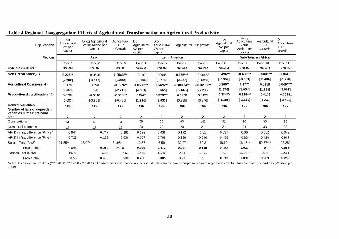
30
Table 4 Regional Disaggregation: Effects of Agricultural Transformation on Agricultural Productivity
Dep. Variable
log Agricultural
VA per capita
D.log Agricultural Value Added per
worker
Agricultural TFP
Growth
log Agricultural VA per capita
Dlog Agricultural VA per capita
Agricultural TFP growth
log Agricultural
VA per capita
D.log Agricultural
Value Added per
worker
Agricultural TFP
Growth
D Agricultural TFP growth
Regions Asia Latin America Sub-Saharan Africa
Case 1 Case 2 Case 3 Case 4 Case 5 Case 6 Case 7 Case 8 Case 9 Case 10 Case 11
EXP. VARIABLES SGMM SGMM SGMM SGMM SGMM SGMM SGMM SGMM SGMM SGMM SGMM
Non Cereal Share(-1) 0.225** -0.0546 0.0583*** -0.197 0.0996 0.165*** -0.00453 -0.494*** -0.498*** -0.0805*** -0.0610*
[2.650] [-0.516] [2.890] [-0.696] [0.274] [2.937] [-0.0981] [-2.957] [-3.569] [-3.484] [-1.756]
Agricultural Openness(-1) 0.170 0.0244 -0.0276** 0.0500*** 0.0426*** -0.00184** -0.00208*** 0.166** 0.177* 0.0188 0.0494***
[1.463] [0.345] [-2.213] [4.561] [5.665] [-2.665] [-7.205] [2.378] [1.854] [1.298] [3.002]
Production diversification (-1) 0.0709 -0.0316 -0.00607 0.247* 0.328*** 0.0278 0.0135 -0.384*** -0.385*** -0.0135 -0.00541
[1.003] [-0.808] [-0.465] [1.916] [3.033] [0.995] [0.876] [-3.365] [-2.921] [-1.232] [-0.301]
Control Variables Yes Yes Yes Yes Yes Yes Yes Yes Yes Yes Yes Number of lags of dependent variables in the right hand side 2 2 2 2 2 2 2 2 2 2 2
Observations 61 43 51 58 56 60 148 91 90 93 93
Number of countries 17 17 18 20 20 20 21 31 31 33 33
AR(1) in first difference (Pr > z ) 0.944 0.747 0.182 0.199 0.036 0.172 0.01 0.037 0.06 0.052 0.042
AR(2) in first difference (Pr>z) 0.723 0.189 0.636 0.067 0.768 0.239 0.596 0.458 0.83 0.426 0.967
Sargan Test (Chi2) 21.55** 18.07** 31.95* 12.57 6.59 30.97 52.2 18.10* 16.45** 50.87*** 28.88*
Prob > chi2 0.043 0.012 0.078 0.199 0.472 0.097 0.135 0.053 0.021 0 0.068
Hansen Test (Chi2) 10.75 6.66 7.61 12.75 12.49 9.53 13.51 9.2 15.00** 25.6 22.51
Prob > chi2 0.55 0.465 0.998 0.238 0.085 0.99 1 0.513 0.036 0.269 0.259
Notes: t-statistics in brackets (*** p<0.01, ** p<0.05, * p<0.1). Standard errors are based on the robust estimator for small sample in regional regressions for the dynamic panel estimations (Windmeijer, 2005)

31
That is, for Sub-Saharan Africa, it would be crucial for policymakers to specialise certain
crop productions, such as cereals, to improve the efficiency through the economies of scale,
and focus on increasing the share of agricultural export in the total agricultural production. 22
(3) Results of Model 3: SDG 1
We now apply the FE-IV model for both five-year average panel in Table 5.23
The model
consists of the two stages: the first stage where log agricultural value added per worker is
estimated by our three measures of agricultural transformation, namely, the
commercialisation index, the agricultural openness index, and the product diversification
index (instruments) with control variables and the second stage where the poverty headcount
ratio is estimated by log of agricultural value added per worker that was estimated in the first
stage. The objective variables are poverty headcount ratios at US$1.9 or US$3.1 a day (2011
PPP) at national levels (Cases 1-2 of Table 5) or US$1.25 or US$2 a day (2005 PPP) at the
national level, or at rural or urban areas (Cases 3-8 of Table 4). In the first stage agricultural
openness is positive and significant in all the cases in Table 4, while the commercialisation is
significant in Cases 1-4 and the product diversification index is significant in Cases 5-8.
Sagan test together with Stock-Yogo test implies that the instruments are valid in all the
cases except Case 8.
Table 5 SDG 1: Effects of Agricultural Transformation on Poverty
Dep. Variable
Poverty HC
USD3.10
Poverty HC
USD1.90
Poverty HC
USD2.00
Poverty HC
USD1.25
Rural Poverty HC USD2.00
Rural Poverty HC USD1.25
Urban Poverty HC USD2.00
Urban Poverty HC USD1.25
Regions All Developing Areas
Data Five Year Average Panel
Case 1 Case 2 Case 3 Case 4 Case 5 Case 6 Case 7 Case 8
EXP. VARIABLES IV IV IV IV IV IV IV IV
FIRST STAGE Dep. Variable log Agricultural value added per worker log Agricultural value added per worker
Commercialization Index
22 We have carried out the same regressions for the balanced panel for the cases where a dependent
variable is log agricultural value added per capita. The results are broadly similar to those in Table 5. 23
The results based on annual panel data are very similar and consistent. Regressions based on the
balanced panel will produce similar results for selective indicators, such as poverty, child
malnutrition and the Gini coefficient. These will be provided on request.

32
L1. -0.682** -0.682** -0.697** -0.697** -0.424 -0.424 -0.424 -0.424
[-2.00] [-2.00] [-2.01] [-2.01] [-1.05] [-1.05] [-1.05] [-1.05]
Agricultural Openness L1. 0.386*** 0.386*** 0.787*** 0.787*** 0.460*** 0.460*** 0.460*** 0.460***
[7.40] [7.40] [7.29] [7.29] [8.59] [8.59] [8.59] [8.59]
Product diversification L1. -0.027 -0.027 -0.121 -0.121 -0.452*** -0.452*** -0.452*** -0.452***
[-0.19] [-0.19] [-0.82] [-0.82] [-2.68] [-2.68] [-2.68] [-2.68]
Control Variables Yes Yes Yes Yes Yes Yes Yes Yes
Poverty HC
USD310
Poverty HC
USD190
Poverty HC
USD200
Poverty HC
USD125
Rural Poverty HC
USD200
Rural Poverty HC
USD200
Urban Poverty HC
USD200
Urban Poverty HC
USD200
VARIABLES
Poverty HC
USD3.10
Poverty HC
USD1.90
Poverty HC
USD2.00
Poverty HC
USD1.25
Rural Poverty HC USD2.00
Rural Poverty HC USD1.25
Urban Poverty HC USD2.00
Urban Poverty HC USD1.25
log Agricultural Value Added per worker -0.162*** -0.079 -0.239*** -0.079 -0.2398*** -0.151*** -0.1471*** -0.0832**
[-2.875] [-1.386] [-3.922] [-1.247] [-4.265] [-2.736] [-3.050] [-1.996]
Control Variables Yes Yes Yes Yes Yes Yes Yes Yes
Observations 371 371 326 326 224 224 224 224
R-squared 0.373 0.265 0.286 0.123 0.351 0.333 0.305 0.193
Number of country 85 85 83 83 74 74 74 74
F test of excluded instruments
F( 3, 279) =
F( 3, 279) =
F( 3, 236) =
F( 3, 236) = F( 3, 143) = F( 3, 143) = F( 3, 143) = F( 3, 143) =
19.79*** 19.79*** 19.09*** 19.09*** 26.40*** 26.40*** 26.40*** 26.40***
Prob > F = 0 0 0 0 0 0 0 0
Sargan statistic
(over identification
test of all instruments) 1.459 3.743 0.722 3.389 3.879 4.263 3.864 6.664**
Chi-sq(2) Pvalue 0.482 0.154 0.697 0.184 0.144 0.119 0.145 0.036
Elasticity Estimates
VARIABLES
Poverty HC
USD3.10
Poverty HC
USD1.90
Poverty HC
USD2.00
Poverty HC
USD1.25
Rural Poverty HC USD2.00
Rural Poverty HC USD1.25
Urban Poverty HC USD2.00
Urban Poverty HC USD1.25
∂Poverty HC /∂ log agrivapw -0.16*** -0.0785 -0.239*** -0.079 -0.2398*** -0.151*** -0.147*** -0.8323** ∂log agrivapw
/∂ Ag Openness 0.386*** 0.386*** 0.787*** 0.787*** 0.460*** 0.460*** 0.460*** 0.460***
∂ Poverty HC /∂Ag openness -0.062*** -0.030 -0.188*** -0.062 -0.110*** -0.069*** -0.068*** -0.038***
z-statistics in brackets. *** p<0.01, ** p<0.05, * p<0.1
The estimates of the elasticity of poverty with respect to agricultural openness (evaluated
at the mean of the poverty headcount ratio) are shown at the bottom of Table 5. The first
conclusion is that agricultural openness tends to reduce poverty more strongly at the higher
poverty thresholds. In other words, the poverty reducing effects at the lower poverty
thresholds are limited. Second, based on the five-year average panel data, a 1% increase in
the agricultural openness tends to reduce poverty ay by 0.062% to 0.188% at higher poverty
thresholds and by 0.03% to 0.06% at the lower thresholds, though the latter are not
statistically significant. These are not high at first sight, but poverty-reducing effects are
likely to be substantial as the effects will be accumulated over the years. Thirdly, agricultural

33
openness is likely to reduce both rural and urban poverty, with the absolute magnitude of
reduction larger for rural poverty. We conclude that the agricultural transformation, proxied
by the agricultural openness, has a significant poverty-reducing effect. We have used the
poverty headcount ratios, but similar conclusions have been obtained for poverty gap
measures. In terms of policy implications, it is important for policymakers to facilitate
agricultural export directly by removing tariff and non-tariff barriers, or indirectly by
investing rural or transport infrastructure to reducing transaction costs, in order to improve
the overall agricultural productivity and eradicate extreme poverty.
(4) Results of Model 3: SDG 2
As we have already examined the effects of agricultural transformation indices on
agricultural productivity in details, we will estimate the effects of agricultural transformation
indices on child malnutrition, undernutrition and food security. The same model, namely, the
FE-IV model is used except the case where the prevalence of undernutrition is estimated as
the predicted value of the log of agricultural value added is not statistically significant in the
second stage. The results are reported in Table 6.
Stock-Yogo test and Sargan test validate our instruments in terms of the relevance and the
exclusion restriction except for Cases 4-6 where the F-statistics are lower than the Stock-
Yogo threshold. In Table 6, the agricultural openness is positive and significant in the first
stage and log agricultural value added per worker is negative and significant in all the cases.
As before, the elasticity estimates are reported at the bottom of Table 6. It is found that an
increase in agricultural openness significantly reduces the prevalence of underweight. A 1%
increase in the agricultural openness leads to 0.038% reduction in the rate of prevalence of
child underweight evaluated at its mean, other factors being equal. Likewise, a 1% increase
in the commercialisation index leads to 0.013% reduction in the rate of prevalence of child
underweight.

34
Table 6 SDG 2: Effects of Agricultural Transformation on Hunger and Food Security (based on Five Year Average Panel) Dep. Variable
Regions
Weight-for-Age
Height-for-Age
Energy_Supply_Adequacy Protein_Supply Depth_Food_Deficit Anaemia_during_Pregnancy Prevalence of under nutrition
Data Five Year Average Panel
Case 1 Case 2 Case 3 Case 4 Case 5 Case 6 Case 7
EXP. VARIABLES IV FE
FIRST STAGE
Dep. Variable log Agricultural value added per worker
Commercialization Index
L1. -0.066 -0.359 -0.369 -0.389 0.239 -0.262 -
[-0.18] [-0.95] [-1.14] [-1.15] [0.67] [-0.83] -
Agricultural Openness
L1. 0.525*** 0.504*** 0.075*** 0.046*** 0.022*** 0.047*** -
[6.95] [6.56] [4.52] [2.23] [1.34] [2.25] -
Product Diversification
L1. -0.092 -0.129 -0.224 -0.103 -0.323 -0.007 -
[-0.67] [-0.91] [-1.65] [-0.73] [-2.45] [-0.05] -
SECOND STAGE
Dep. Variable
Weight-for-Age
Height-for-Age
Energy_Supply_Adequacy Protein_Supply Depth_Food_Deficit Anaemia_during_Pregnancy Prevalence of under nutrition
Commercialization Index -9.314
L1. [-0.990]
Agricultural Openness -0.0061
L1. [-1.527]
Product Diversification 4.503
[1.379]
log Agricultural Value Added per worker
-0.073*** -0.195*** 0.171*** 0.2671*** -1.307** -0.205** -
[-3.057] [-4.695] [4.249] [3.068] [-2.191] [-2.422]
Control Variables Yes Yes Yes Yes Yes Yes Yes
Observations 373 367 515 414 447 439 389
R-squared 0.51 0.306 0.363 0.029 0.332 -0.225 0.330
Number of country 87 87 98 91 82 96 80

35
F test of excluded instruments
F( 3, 279) = F( 3, 273) =
F( 3, 410) = F( 3, 316) = F( 3, 358) = F( 3, 336) = -
16.24*** 15.25*** 8.18*** 2.26* 2.73 1.93
Prob > F = 0 0 0 0.0814 0.0438 0.1252
Sargan statistic
(over identification
test of all instruments) 1.618 2.201 1.216 1.38 0.587 0.669
Chi-sq(2) Pvalue 0.4454 0.3328 0.5445 0.5016 0.7456 0.7156
Elasticity estimates Weight-for-
Age Height-for-Age
Energy_Supply_Adequacy Protein_Supply Depth_Food_Deficit Anaemia_during_Pregnancy Prevalence of
under nutrition
∂SDG2/∂log agrivapw -0.073*** -0.195*** 0.171*** 0.267*** -1.307*** -0.205*** -
∂log agrivapw 0.525*** 0.504*** 0.075*** 0.046*** 0.022*** 0.047***
-
/Ag Openness
∂SDG2 /∂ Ag openness
-0.038*** -0.098*** 0.013*** 0.012*** -0.029*** -0.010*** -0.006
z-statistics in brackets. *** p<0.01, ** p<0.05, * p<0.1.

36
We also found that a 1% increase in the agricultural openness on average leads to 0.098%
reduction in the rate of prevalence of stunting evaluated at its mean, other factors being
equal. We have also confirmed that if agricultural sector is more open to the rest of the
economy, food security is likely to improve in a number of dimensions, such as energy
supply adequacy, protein supply and (lack of) food deficit and the rate of pregnant women
who suffer from anaemia. In the final column, the result is presented on the prevalence of
undernutrtion (POU). It is found that if agricultural openness increases by 1%, the POU tends
to decrease by 0.006. However, the result should be interpreted with caution as it is not
statistically significant.
(5) Results of Model 3: SDG 10
Next, we have estimated the effects of agricultural transformation on inequality (SDG 10)
using the Gini coefficient at national, rural and urban levels as well as welfare growth rate of
the bottom 40% in Table 7. While the FE-IV model is applied to the Gini, a simple single
univariate model is used for the growth of the bottom 40% of the population. Instruments
have been validated in all the cases in terms of the instrument relevance test (Stock-Yogo
test) and the test for exclusion restrictions (Sargan Test).
Table 7 SDG 10: Effects of Agricultural Transformation on Inequality
Dep. Variable Gini Rural Gini
Urban Gini
Growth Rate of Bottom
40%
Regions All developing areas
Data Five-year average panel
Case 1 Case 2 Case 3 Case 4
EXP. VARIABLES IV OLS
FIRST STAGE Dep. Variable
Commercialization Index
L1. -0.243 -0.272 -0.270 -
[-0.79] [-0.57] [-0.56]
Agricultural Openness
L1. 0.419*** 0.438*** 0.439***
[9.51] [5.25] [5.21]
Product Diversification L1. -0.051 0.152 0.152

37
[0.36] [0.69] [0.68]
Control Variables Yes Yes Yes -
SECOND STAGE
Dep. Variable Gini Rural Gini Urban Gini
Growth Rate of Bottom
40%
log Agricultural Value Added per worker -0.066*** -0.069* -0.061 -0.784**
[-2.835] [-1.680] [-1.507] [-2.327]
Control Variables Yes Yes Yes -
Observations 303 72 71 R-squared 0.056 0.166 0.144 Number of countries 91 22 22
F test of excluded instruments
F( 3, 204) =
F( 3, 43) =
F( 3, 42) = -
30.52*** 9.67*** 9.51***
Prob > F = 0 1E-04 1E-04 Sargan statistic
(over identification test of all
instruments) 2.841 3.275 1.652 Chi-sq(2) Pvalue 0.242 0.194 0.438
Elasticity Estimates Gini Rural Gini Urban Gini
Growth Rate of Bottom
40%
∂Gini/∂log agrivapw -0.066*** -0.069*** -0.061*** ∂log agrivapw
/∂Ag Openness 0.419*** 0.438*** 0.439***
∂Gini /∂Ag openness -0.028*** -0.030*** -0.027***
Table 7 shows that one of the instruments, agricultural openness is positive and significant
in the first stage in all the cases where FE-IV model is applied, while log agricultural value
added per worker is negative and significant in the second stage regression for the Gini
coefficient. The combined elasticity estimates are shown at the bottom of Table 7. A 1%
increase in the agricultural openness corresponds to 0.028% decline in the national Gini,
0.03% decline in the rural Gini and 0.027% decline in the urban Gini. This appears not to be
large at first sight, but cumulative effects could be substantial. That is, the agricultural
transformation is found to have a substantial inequality-reducing effect.
However, we have found a negative and significant relationship between log agricultural
value added per worker and the welfare growth rate of bottom 40%. That is, agricultural
growth tends to deter the welfare growth of bottom 40%. Given that the main determinant of
agricultural value added per worker is agricultural openness, we can infer that agricultural
transformation in terms of increased openness of the agricultural sector to the rest of the

38
world would increase inequality once we focus on the growth rate of bottom 40%. However,
because this is a crude measure of inequality that ignores the distribution among the bottom
40%, we would place more importance on the results which confirm inequality-reducing
effects of agricultural transformation when the Gini coefficient is applied.
We have confirmed that the agricultural openness is significantly associated with
improvement in a number of measures in SDGs 1, 2 and 10. However, a caveat is that not all
the countries have been successful in increasing the agricultural openness. In most of the
countries in Latin America and Sub-Saharan Africa, the index increased only gradually as
indicated by graphs in Appendix 7. Overall, the agricultural openness index increased by
1.7% annually (by 1.0% for Asia, 3.1% for Latin America and by 1.1% for Sub-Saharan
Africa). But this average masks the heterogeneity across different countries as while some
countries have managed to increase the agricultural openness greatly, agricultural openness
remained unchanged in some countries. For instance, Botswana (South Africa) increased the
agricultural openness by 5.8% (2.9%) annually, while it was stagnant in other SSA countries.
In Asia, Malaysia or Vietnam has had a high growth rate in the agricultural openness (3.3%
and 2.9% respectively), but the increase is slow in South Asian countries. Hence how the
country changes the export structure strategically is key to embodying a positive effect of the
agricultural openness on SDGs.
(5) Results of Model 3: SDG 1 and 2 at regional levels
To see how other indices affect SDGs, we have estimated the Model 3 where in the first
stage the dynamic model is used and in the second the fixed effects model is applied by using
the predicted values of log agricultural value added and the error term with standard errors
bootstrapped. This is carried out for selective cases of regional regressions for Asia, Latin

39
America, and Sub-Saharan Africa where insightful results are obtained in the first stage. The
results are reported in Table 8.
We have found that for Asia the lagged share of non-cereal production significantly
reduces poverty headcounts at US$3.10 and US$1.90 as well as the prevalence of stunting
and underweight. For instance, a 1% increase in the lagged share of non-cereal production
reduces poverty at US$3.10 by 0.12%. In Latin America, on the other hand, the product
diversification index significantly reduces the poverty headcount at US$3.10. A 1% increase
in the diversity index leads to, on average, 0.085% decline in the poverty headcount at
US$3.10. While this is larger than the effect of the agricultural openness (0.0074%), we
avoid comparing the estimates across different measures of agricultural transformation as a
1% change has a different meaning according to which index we focus on. In Sub-Saharan
Africa, though the estimates are statistically insignificant, an increase in the cereal share is
likely to decrease poverty, the results which are in sharp contrast with those for Asia.
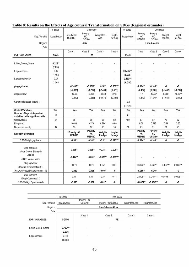
40
Table 8: Results on the Effects of Agricultural Transformation on SDGs (Regional estimates)
1st Stage 2nd stage 1st Stage 2nd stage
Dep. Variable logagrivapw Poverty HC
USD310
Poverty HC
USD190
Weight-for-Age
Height-for-Age
logagrivapw Poverty
HC USD310
Poverty HC
USD190
Weight-for-Age
Height-for-Age
Regions Asia Latin America
Data
Case 1 Case 2 Case 3 Case 4 Case 1 Case 2 Case 3 Case 4
EXP. VARIABLES SGMM FE SGMM FE
L.Non_Cereal_Share 0.225** - - - - - - - - -
[2.650]
L.agopenness 0.17 - - - - 0.0405*** - - - -
[1.463]
[6.078]
L.productdiversity 0.07 - - - - 0.463*** - - - -
[1.003]
[6.019]
plogagrivapw -0.5497** -0.3619* -0.10** -0.230*** -0.184** -0.105** -0 -0
[-2.375] [-1.722] [-2.489] [-3.211] [-2.457] [-2.063] [-1.432] [-1.292]
elogagrivapw -16.68 -8.155 -4.848 2.18 -17 -13.28* -5.385* -10.70**
[-0.440] [-0.238] [-0.676] [0.147] [-1.549] [-1.749] [-1.654] [-2.010]
Commercialisation Index(-1)
-0.2
[-1.121]
Control Variables Yes Yes Yes Yes Yes Yes Yes Yes Yes Yes
Number of lags of dependent variables in the right hand side
2 - - - - 2 - - - -
Observations 61 69 69 65 62 100 87 87 76 72
R-squared 0.463 0.378 0.794 0.69 0.56 0.513 0.53 0.65
Number of country 17 17 17 18 18 21 21 21 21 21
Elasticity Estimates Poverty HC
USD310
Poverty HC
USD190
Weight-for-Age
Height-for-Age
Poverty
HC USD310
Poverty HC
USD190
Weight-for-Age
Height-for-Age
∂ SDG/ ∂ plogagrivapw - -0.55** -0.362* -0.1** -0.023*** - -0.184** -0.105** -0 -0
∂log agrivapw 0.225** 0.225** 0.225** 0.225** - - - -
/∂Non Cereal Share(-1)
∂ SDG -0.124** -0.081* -0.023** -0.005*** - - - -
/∂Non_cereal share
∂log sgrivapw/ 0.071 0.071 0.071 0.07 0.463*** 0.463*** 0.463*** 0.463***
∂Product diversification (-1)
∂ SDG/dProduct diversification (-1) -0.039 -0.026 -0.007 -0 -0.085** -0.049 -0 -0
∂log agrivapw 0.17 0.17 0.17 0.17 0.0405*** 0.0405*** 0.0405*** 0.0405***
/∂Agri Openness(-1)
∂ SDG/ ∂Agri Openness(-1) -0.093 -0.062 -0.017 -0 -0.0074** -0.0043** -0 -0
1st Stage 2nd stage
Dep. Variable logagrivapw Poverty HC
USD310 Poverty HC USD190 Weight-for-Age Height-for-Age
Regions Sub-Saharan Africa
Data
Case 1 Case 2 Case 3 Case 4
EXP. VARIABLES SGMM FE
L.Non_Cereal_Share -0.702*** - - - -
[-2.994]
L.agopenness 0.115 - - - -
[1.348]

41
L.productdiversity 0.138 - - - -
[1.527]
plogagrivapw -0.1364 -0.2246* -2.809 -0.526
[-1.580] [-1.785] [-1.300] [-0.173]
elogagrivapw -10.27 -23.09 0.265 7.175*
[-0.792] [-1.280] [0.123] [1.804]
Commercialisation Index(-1) -13.64 -22.46* -2.809 -0.526
[-1.580] [-1.785] [-1.300] [-0.173]
Control Variables Yes Yes Yes Yes Yes Number of lags of dependent variables in the right hand side 2
Observations 124 96 96 124 125
R-squared 0.255 0.317 0.348 0.289
Number of country 32 33 33 34 34
Elasticity Estimates Poverty HC USD310 Poverty HC
USD190 Weight-for-
Age Height-for-Age
∂ SDG/ ∂ plogagrivapw - -0.1364 -0.2246* -0.028 -0.0053
∂log agrivapw
/∂Non Cereal Share(-1) -0.702*** -0.702*** -0.702*** -0.702*** ∂ SDG
/∂Non_cereal share 0.096 0.158* 0.020 0.004
∂log sgrivapw/ ∂Product diversification (-1) 0.138 0.138 0.138 0.138
∂ SDG/dProduct diversification (-1) -0.019 -0.031 -0.004 -0.001
∂log agrivapw /∂Agri Openness(-1) 0.115 0.115 0.115 0.115
∂ SDG/ ∂Agri Openness(-1) -0.0157 -0.0258 -0.0032 -0.0006
z-statistics in brackets. *** p<0.01, ** p<0.05, * p<0.1.
VI. Concluding Remarks and Policy Implications
This paper has analysed the role of the transformation of the rural agricultural sector (or
‘agricultural transformation’ in short) in achieving Sustainable Development Goals (SDGs)
1, 2 and 10 drawing upon the cross-country panel data over the past four decades for 105
developing countries. Agricultural transformation has been featured in recent years as an
important change in the agricultural sector and in the rural economies of developing
countries as the rural agriculture sector has become closely linked to not only the non-
agricultural or industrial sector of the country and the rapidly-growing urban sector of the
country but also the agricultural and non-agricultural sectors of both developed and
developing countries.
The process of agricultural transformation is diverse and it is not straightforward to
quantify it in a meaningful way. So we define agricultural transformation by three different
42
indices, namely, (i) the agricultural openness index - the share of agricultural export in
agricultural value added of the country, (ii) the commercialization index - the share of
processed agricultural products, fruits, green vegetables, and meats in all primary and
processed agricultural products, and (iii) the product diversification index to capture the
extent to which the country diversify the agricultural production.
Agricultural development has been considered to be important for poverty reduction, but
it remains unclear whether agricultural transformation influences agricultural development
and poverty, SDG 1. Also important yet unclear is whether and the extent to which
agricultural transformation would reduce hunger, malnutrition and food security (SDG 2) and
inequality (SDG 10). Our study is important because, as far as we know, this is the first study
to quantify the agricultural transformation - even in a limited manner - and evaluate its effect
on agricultural productivity and SDGs. Methodologically, not only the dynamic nature of
agricultural production but also the endogeneity of agricultural transformation is taken into
account by the model of system Generalized Method of Moments (system GMM).
First, we have found that transformation of the agricultural sector in terms of agricultural
openness has dynamically increased the broad measure of agricultural productivity (in terms
of agricultural value added per worker) and its growth and has consequently reduced
national, rural and urban poverty significantly. However, the poverty-reducing effects of the
agricultural transformation are relatively larger at the higher poverty thresholds (US$3.1 per
day (2011PPP) and US$2 per day (2005PPP)) than at the lower poverty thresholds (US$1.9
per day (2011PPP) and US$1.25 per day (2005PPP)) for both poverty headcount and poverty
gap measures. So there is a possibility that the moderately poor benefit more than the
extremely poor from the process of agricultural transformation. Our results may be driven by
a cluster of countries with relatively high growth in both agricultural openness and

43
agricultural productivity and so the results will have to be interpreted with caution given that
it may not be straightforward to the country increases agricultural openness in a short period.
Second, agricultural openness is negatively associated with child malnutrition in terms of
underweight and stunting, improves food security measures, such as the indices of energy
supply adequacy, protein supply, depth of food deficit and the prevalence of anaemia among
pregnant women.
Third, the agricultural openness tends to reduce the Gini coefficient at both national and
subnational levels (for both rural and urban areas), while it is likely to deter the welfare
growth of the bottom 40%. So we have good evidence to support the claim that agricultural
transformation in terms of agricultural openness helps achieve SDG 1 (poverty reduction),
SDG 2 (reducing hunger and malnutrition, improving food security, and doubling
agricultural productivity) and SDG 10 (reducing inequality).
Fourth, whether more commercialisation in terms of the higher share of processed crops,
fruits and green vegetables improves agricultural production depending on the specifications
and geographical regions. For instance, if we use pooled OLS or random effects model, the
higher commercialisation index is associated with higher agricultural value added per
worker. Also, in Latin America where the agricultural sector is more mature than other
regions, commercialisation tends to improve agricultural TFP. In a few cases the
commercialisation index is negative and significant. This could be due to the fact that fact
that the higher commercialisation captures the lower share of cereal production. In one case,
the higher share of cereal crops – together with agricultural openness – was found to
increases log agricultural value added per worker (particularly in Sub-Saharan Africa and
Latin America).
Fifth, product diversification, contrary to our expectation, reduces agricultural
productivity in a number of cases. This is likely to be due to the fact that the economies of

44
scale of agricultural production are often important in raising the country’s agricultural
productivity. Also, if similar crops are produced in a large area of the country, positive effect
on productivity due to learning from one region to another, or competition across different
regions is greater. For instance, among Asian countries, Malaysia has achieved a higher
agricultural productivity with the low product diversification (Imai, Gaiha, and Bresciani,
2016). However, among Latin American countries, product diversification was found to
increase agricultural productivity.
Our study has a number of policy implications. First, agricultural productivity growth,
for instance, through higher agricultural openness will help developing countries achieve
SDG 1 (poverty reduction), SDG 2 (alleviation of malnutrition and hunger; securing food
security), and SDG 10 (reduction of inequality). Because SDG 2 includes doubling
agricultural productivity, our analysis suggests a win-win solution where the facilitation of
agricultural trades, for instance, through promoting regional economic integrations, reducing
transaction costs such as tariff and non-tariff barriers, would improve agricultural
productivity and address other SDG goals of poverty, hunger and inequality. However, if the
country’s agricultural openness has become already high (e.g. Thailand, Vietnam), there is
no scope for increasing the agricultural openness and a policy is crucial to further increase
the agricultural productivity or directly support the poor. If the country’s agricultural
openness is low, it can increase the agricultural productivity by promoting the agricultural
export, which could indirectly improve SDG measures. However, it should be noted that the
effects of agricultural openness on SDGs are indirect. What is crucial is for the country to
choose a set of policies to maximise agricultural productivity (where increasing the openness
is only one of the potential choices) in order to achieve SDGs.
Second, our paper shows that agricultural transformation is likely to improve agricultural
productivity, which would reduce both moderate poverty and extreme poverty. However, the

45
poverty-reducing effect is higher for the former. It is noted here that agricultural
transformation itself does not have any distributional effect. Agricultural productivity
improvement will bring about benefits for the moderate poor, rather than the extreme poor,
because the latter may be left out of the process of accessing the new technologies,
infrastructure, or other opportunities for agricultural transformations. Under these
circumstances, a policy is still important to support the poorest while the rural agricultural
sector undergoes a transformation. Also, given that there is a negative correlation between
the agricultural value added per worker and the welfare growth of the bottom 40%, the
eventual/indirect distributional impact of policies promoting the process of agricultural
transformation should be carefully monitored.
Third, our results suggest that product specialisation is important for improving
agricultural productivity, except for Latin America.24
This could be related to other findings
of the current study, such as an important role of agricultural openness - where the neo-
classical trade theory implies higher efficiency through specialisations - as well as the
importance of cereal production in improving overall productivity. Depending on the stage of
agricultural development, facilitating the production and exporting of cereal crops will
increase the agricultural productivity, while at the higher level of development (e.g. Latin
America), product diversification would increase agricultural productivity.
Finally, if efficiency though the economies of scale is important - suggested by the roles
of product specification (which are implied by negative coefficient estimates of product
diversifications in several cases e.g. in Tables 3 and 4) - there is a case for promoting synergy
between public and private investment in rural areas and for improving the quality of rural
infrastructure. A priority is to strengthen rural infrastructure. Our results suggest that the
transformation process incorporating poor smallhoders through easier access to credit, land
24
It is noted that regional regressions in Table 4 show negative coefficient estimates of product
diversification for Asia and Sub-Saharan Africa.
46
and output markets leads to poverty and inequality reduction. As prospects of absorption of
growing rural labour force in manufacturing and services and other activities are limited, job
expansion in rural areas is imperative. Some of the preceding proposals would help create
more employment in rural areas, raise wage rates and dampen rural-urban migration. Land
rental markets would facilitate the redistribution of land in favour of more efficient small
farmers and help consolidation of small farms into more viable units.
There are broadly three directions in the future research. First, the future research needs
to utilise the micro-level household dataset to construct the indices on agricultural
transformation (e.g. product diversification index at farm levels) and examine the effects of
transformation on SDGs. Second, given the complexity of agricultural transformation, it will
be useful to refine the variables on agricultural transformation by focusing on different
aspects (e.g. FDI in food sectors). Third, our study has clearly shown that agricultural
transformation improves SDGs, but the transformation alone will not be sufficient for
achieving goals (e.g. eradicating extreme poverty or doubling agricultural productivity). We
then need to examine more carefully the success cases (e.g., China, Viet Nam, Malaysia,
Thailand) which managed to more than double the agricultural TFP in 1961-2012. Given the
regional heterogeneity, in depth cross-country on the effects of agricultural transformation on
agricultural productivity will be helpful in order to further disentangle the complex
causalities between agricultural transformation and SDGs.
References
Alston, J.M. and Pardey, P.G, (2014). Agriculture in the global economy. The Journal of
Economic Perspectives, 28(1), pp.121-146.
Arellano, M., and Bond, S, (1991)Some tests of specification for panel data: Monte Carlo
evidence and an application to employment equations. Review of Economic Studies 58:
277-297.

47
Arellano, M. and O. Bover. (1995). Another look at the instrumental variable estimation of
error-components models. Journal of Econometrics 68: 29-51.
Baltagi, B.H. and Chang, Y.J. (1994). Incomplete panels: A comparative study of alternative
estimators for the unbalanced one-way error component regression model. Journal of
Econometrics, 62(2), pp.67-89.
Baltagi, B.H. and Song, S.H., (2006). Unbalanced panel data: A survey. Statistical Papers,
47(4), pp.493-523.
Baldé, Y., (2011). The impact of remittances and foreign aid on savings/investment in Sub‐
Saharan Africa. African Development Review, 23(2), pp.247-262.
Blundell, R., and S. Bond. (1998). Initial conditions and moment restrictions in dynamic
panel data models. Journal of Econometrics 87: 115-43.
Ba, M.B., Staatz, J. M., Farrelly, L. L., Camara, Y., Dimithe, G. (1999) ‘Workshop on
Agricultural Transformation in Africa: Abidjan, Côte D'Ivoire, September 26-29,
1995’, Food Security International Development Working Papers 54668, Michigan
State University, Department of Agricultural, Food, and Resource Economics.
Barrett, C. B., M. E. Bachke, M. F. Bellemare, H. C. Michelson and S. Narayanan (2012)
‘Smallholder Participation in Contract Farming: Comparative Evidence from Five
Countries’ World Development, 40(4), pp.715-730.
Barrett, C.B., Christiaensen, L., Sheahan, M. and Shimeles, A., (2017) On the structural
transformation of rural Africa. Journal of African Economies, 26(suppl_1), pp.i11-i35.
Bloom, D. E., Canning, D., Fink, G., Finlay, J. (2007). ‘Realizing the Demographic
Dividend: Is Africa any different?’ PGDA Working Paper No. 23, Harvard University.
Blundell, R., and S. Bond (1998). Initial conditions and moment restrictions in dynamic
panel data models.Journal of Econometrics 87: 115-143.

48
Chiodi, V., Jaimovich, E. and Montes-Rojas, G. (2012). Migration, remittances and capital
accumulation: Evidence from rural Mexico. Journal of Development Studies, 48(8),
pp.1139-1155.
Christiaensen, L., Demery, L., and Kuhl, J. (2011). 'The (Evolving) Role of Agriculture in
Poverty Reduction—An Empirical Perspective', Journal of Development Economics,
96 (2), 239-54.
Dawe, D. (2015) ‘Agricultural transformation of middle-income Asian economies:
diversification, farm size and mechanization’, ESA Working Paper 15-04, Rome, FAO.
de Janvry, A. and Sadoulet, E. (2009). Agricultural growth and poverty reduction: Additional
evidence. The World Bank Research Observer, 25(1), pp.1-20.
Dollar, D., Kleineberg, T. and Kraay, A., 2016. Growth still is good for the poor. European
Economic Review, 81, pp.68-85.
FAO (2011) ‘Crops statistics: Concepts, definitions and classifications’, mimeo, Rome, FAO.
FAO (2014) FAO Statistical Programme of Work 2014-15, Rome, FAO,
Fuglie, K. O. (2012). ‘Productivity Growth and Technology Capital in the Global
Agricultural Economy.’ In: Fuglie K., Wang, S.L. and Ball, V.E. (eds.) Productivity
Growth in Agriculture: An International Perspective. CAB International, Wallingford,
UK, pp. 335-368.
Fuglie, K. O. (2015). ‘Accounting for Growth in Global Agriculture,’ Bio-based and Applied
Economics, vol. 4 (December).
Headey, D., Bezemer, D., and Hazell, P. B. (2010). ‘Agricultural Employment Trends in
Asia and Africa: Too Fast or Too Slow?’, World Bank Research Observer, 25:57–89.
IFAD, WFP, and FAO (2012) The State of Food Insecurity in the World Economic growth is
necessary but not sufficient to accelerate reduction of hunger and malnutrition, FAO,
Rome (http://www.fao.org/docrep/016/i3027e/i3027e.pdf).

49
Imai, K. S., Gaiha, R., and Bresciani, F. (2016) ‘Dynamics of Rural Transformation and
Poverty in Rural Asia and the Pacific’, RIEB Discussion Paper, DP2016-30.
Imai, K. S., Cheng, W. and Gaiha, R. (2017). ‘Dynamic and Long-term Linkages among
Agricultural and Non-Agricultural Growth, Inequality and Poverty in Developing
Countries’, International Review of Applied Economics, 31(3), 318-338.
Imai, K.S., Malaeb, B., and Bresciani, F. (2016). ‘Remittances, Growth and Poverty
Reduction in Asia - A Critical Review of the Literature and the New Evidence from
Cross-country Panel Data’, Draft, IFAD.
Kim, K., Chavas, J. P., Barham, B., & Foltz, J. (2012). Specialization, diversification, and
productivity: a panel data analysis of rice farms in Korea. Agricultural Economics,
43(6), 687-700.
Thirtle, C., Lin, L. and Piesse, J. (2003). The impact of research-led agricultural productivity
growth on poverty reduction in Africa, Asia and Latin America. World Development,
31(12), pp.1959-1975.
Ravallion, M., Chen, S., and Sangraula, P. (2009). “Dollar a Day Revisited,” World Bank
Economic Review, 23(2), pp.163-184.
Remans, R., Wood, S. A., Saha, N., Anderman, T. L,, DeFries, R. S., (2014). ‘Measuring
nutritional diversity of national food supplies’, Global Food Security, 3(3-4), pp.174–
182.
Reardon T and Timmer CP. 2014. “Five Inter-Linked Transformations in the Asian Agrifood
Economy: Food Security Implications.” Global Food Security 3(2): 108-117.
Roodman, D. (2009). How to Do xtabond2: An Introduction to "Difference" and "System"
GMM in Stata. Stata Journal 9(1): 86-136.
Stock, J.H. and Yogo, M. (2005). Testing for Weak Instruments in Linear IV Regression. In
D.W.K. Andrews and J.H. Stock, eds. Identification and Inference for Econometric

50
Models: Essays in Honor of Thomas Rothenberg. Cambridge: Cambridge U y Press,
2005, pp. 80-108. Working paper version: NBER Technical Working Paper 284.
http://www.nber.org/papers/T0284.
Asia: A Synthesis of Issues, Lessons and Policy Implications’, APR, IFAD.
Windmeijer, F. (2005). ‘A finite sample correction for the variance of linear efficient two-
step GMM estimators’. Journal of Econometrics, 126: 25-51.
World Bank (2015). Staying the Course: World Bank East Asia and Pacific Economic
Update October 2015, Washington DC., The World Bank.

51
Appendix 1: Details of Commercialisation Index
The commercialisation index is defined as:
[{Monetary value of production for aggregate crops processed (i.e. beer, cotton lint, cotton
seed, margarine, molasses, oil (such as coconut oil, cottonseed oil, ground nut oil, linseed
oil), palm kernels, sugar raw centrifugal, wine)} + {Monetary value of Production for
Aggregate livestock processed (butter, cheese, milk, lard, yogurt)} + {Monetary value of
production of green vegetables, fruits and derived products, and meat}]
/ [Monetary value of all the primary and processed crops and livestock]
The monetary value of production for aggregate crops processed is calculated by combining
the data on production quantity on ‘Crops processed’
(http://www.fao.org/faostat/en/#data/QD) and ‘Producer prices’
(http://www.fao.org/faostat/en/#data/PP and (http://www.fao.org/faostat/en/#data/PA).25
We
also use the data on the value of agricultural production
(http://www.fao.org/faostat/en/#data/QV) where the monetary values have been already
derived from the price and quantity data files. The values are adjusted based on producer
prices in the international US$ (PPP - Purchasing Power Parity) in 2004-2006.
This measure is based on the assumption that processed agricultural products are more likely
to be commercialized. Below we provide the lists of processed/unprocessed crops and
livestock.
Processed crops:
Margarine, short Sugar Raw Centrifugal Molasses Oil, soybean Oil,
groundnut Oil, coconut (copra) Palm kernels Oil, palm Oil, palm kernel Oil,
olive, virgin Oil, sunflower Oil, rapeseed Oil, safflower Oil, sesame Green vegetable
tallow Oil, stillingia Cottonseed Oil, cottonseed Oil, linseed Beer of barley
Wine Oil, maize Cotton lint
Primary crops:
Fruits and Green vegetables: Total Green vegetables Primary, dry Green vegetables
& Melons, Total Fruit excl Melons, Cabbages and other brassicas Tomatoes
Cauliflowers and broccoli Cucumbers and gherkins Onions, dry Garlic
Peas, green Carrots and turnips Barley Green vegetables, fresh nes Apples
Pears Quinces Apricots Cherries, sour Cherries Peaches and
nectarines Plums and sloes Fruit, stone nes Berries nes, Fruit, tropical fresh
nes Fruit, fresh nes
Non Fruits or Green vegetables: Cereals, nes Potatoes Wheat Sugar beet
Cereals,Total Roots and Tubers,Total Pulses,Total Treenuts, Beans,
Total Coarse Grain, Total Cereals (Rice Milled Eqv) Peas, dry Lentils Pulses, nes
Walnuts, with shell Hazelnuts, with shell Maize Grapes Watermelons
Figs Forage and silage, maize Forage products Green vegetables
and roots fodder Rye Oats
25
However, a limitation of the index is that prices have missing observations and thus cannot be fully
matched with the crop quantity data.
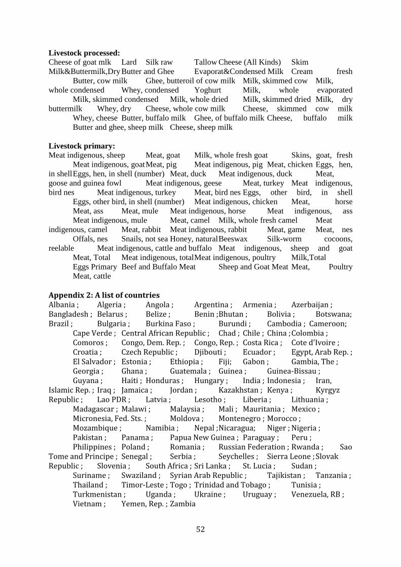
52
Livestock processed:
Cheese of goat mlk Lard Silk raw Tallow Cheese (All Kinds) Skim
Milk&Buttermilk,Dry Butter and Ghee Evaporat&Condensed Milk Cream fresh
Butter, cow milk Ghee, butteroil of cow milk Milk, skimmed cow Milk,
whole condensed Whey, condensed Yoghurt Milk, whole evaporated
Milk, skimmed condensed Milk, whole dried Milk, skimmed dried Milk, dry
buttermilk Whey, dry Cheese, whole cow milk Cheese, skimmed cow milk
Whey, cheese Butter, buffalo milk Ghee, of buffalo milk Cheese, buffalo milk
Butter and ghee, sheep milk Cheese, sheep milk
Livestock primary:
Meat indigenous, sheep Meat, goat Milk, whole fresh goat Skins, goat, fresh
Meat indigenous, goat Meat, pig Meat indigenous, pig Meat, chicken Eggs, hen,
in shell Eggs, hen, in shell (number) Meat, duck Meat indigenous, duck Meat,
goose and guinea fowl Meat indigenous, geese Meat, turkey Meat indigenous,
bird nes Meat indigenous, turkey Meat, bird nes Eggs, other bird, in shell
Eggs, other bird, in shell (number) Meat indigenous, chicken Meat, horse
Meat, ass Meat, mule Meat indigenous, horse Meat indigenous, ass
Meat indigenous, mule Meat, camel Milk, whole fresh camel Meat
indigenous, camel Meat, rabbit Meat indigenous, rabbit Meat, game Meat, nes
Offals, nes Snails, not sea Honey, natural Beeswax Silk-worm cocoons,
reelable Meat indigenous, cattle and buffalo Meat indigenous, sheep and goat
Meat, Total Meat indigenous, total Meat indigenous, poultry Milk,Total
Eggs Primary Beef and Buffalo Meat Sheep and Goat Meat Meat, Poultry
Meat, cattle
Appendix 2: A list of countries Albania ; Algeria ; Angola ; Argentina ; Armenia ; Azerbaijan ; Bangladesh ; Belarus ; Belize ; Benin ; Bhutan ; Bolivia ; Botswana; Brazil ; Bulgaria ; Burkina Faso ; Burundi ; Cambodia ; Cameroon; Cape Verde ; Central African Republic ; Chad ; Chile ; China ; Colombia ; Comoros ; Congo, Dem. Rep. ; Congo, Rep. ; Costa Rica ; Cote d'Ivoire ; Croatia ; Czech Republic ; Djibouti ; Ecuador ; Egypt, Arab Rep. ; El Salvador ; Estonia ; Ethiopia ; Fiji; Gabon ; Gambia, The ; Georgia ; Ghana ; Guatemala ; Guinea ; Guinea-Bissau ; Guyana ; Haiti ; Honduras ; Hungary ; India ; Indonesia ; Iran, Islamic Rep. ; Iraq ; Jamaica ; Jordan ; Kazakhstan ; Kenya ; Kyrgyz Republic ; Lao PDR ; Latvia ; Lesotho ; Liberia ; Lithuania ; Madagascar ; Malawi ; Malaysia ; Mali ; Mauritania ; Mexico ; Micronesia, Fed. Sts. ; Moldova ; Montenegro ; Morocco ; Mozambique ; Namibia ; Nepal ; Nicaragua; Niger ; Nigeria ; Pakistan ; Panama ; Papua New Guinea ; Paraguay ; Peru ; Philippines ; Poland ; Romania ; Russian Federation ; Rwanda ; Sao Tome and Principe ; Senegal ; Serbia ; Seychelles ; Sierra Leone ; Slovak Republic ; Slovenia ; South Africa ; Sri Lanka ; St. Lucia ; Sudan ; Suriname ; Swaziland ; Syrian Arab Republic ; Tajikistan ; Tanzania ; Thailand ; Timor-Leste ; Togo ; Trinidad and Tobago ; Tunisia ; Turkmenistan ; Uganda ; Ukraine ; Uruguay ; Venezuela, RB ; Vietnam ; Yemen, Rep. ; Zambia

53
Appendix 3. Definitions and Descriptive Statistics of Variables
Five-year average data
Variable Definition N Mean SD Min Max
log Agricultural Value Added per worker Agriculture value added per worker
776 7.58 1.2 4.94 12.43
(constant 2010 US$)
Agricultural Value Added per worker log of Agricultural Value Added per worker
776 4389.08 11875.94 140.17 2.50E+05
Commercialisation Index Commercialization Index*1 (FAOSTAT) 1265 0.68 0.18 0.17 0.99
Agricultural Openness [aggregate agricultural export] 831 0.36 0.82 0 13.17
/ [agricultural value added] (FAOSTAT)
Production diversity Product diversification Index *2 (FAOSTAT) 1265 2.54 0.49 0.27 3.4
Non-Cereal_Share The share of non-cereal product production in total agricultural value added 1440 0.42 0.44 0 1
Agricultural TFP Growth Agricultural TFP Index (log) based on FAOSTAT (Fuglie, 2012 and 2015). 1229 0.01 0.02 -0.14 0.15
Land Area Land area (sq. km) 1410 7.58E+05 1.92E+06 460 1.64E+07
Population Density Population density (people per sq. km of Land Area area)
1404 75.49 105.33 0.78 1245.11
Fragility Index State fragility index (= cspf_sfi) 446 11.22 5.88 0 23.8
CPIA rating of macroeconomic management
and coping with fragility (1=low to 6=high)
Trade Openness The share of exports and imports of goods in GDP. 1109 70.26 36.79 4.3 229.64
The percentage of the working age population with 1428 0.73 0.42 0 1
an intermediate level of education
Labour Force with Secondary Education The percentage of the working age population with
1428 0.73 0.42 0.00 1.00
an intermediate level of education
Urban Agglomerations Population in urban agglomerations of more than 894 17.1 11.08 1.19 49.97
1 million (% of total population
Transport Equipment Machinery and Transport Equipment 575 7.59 7.71 0 41.88
(% of value added in manufacturing)
Tariff for primary goods Tariff rate, applied, weighted mean, primary products (%) 556 8.75 8.01 0 55.48
Poverty headcount ($3.1 a day) Poverty headcount ratio at $3.10 a day (2011 PPP)
483 38.6 31 0 98.35
Poverty headcount ($1.9 a day) Poverty headcount ratio at $1.90 a day (2011 PPP)
483 23.09 24 0 94.05
Poverty headcount ($2 a day) Poverty headcount ratio at $2.00 a day (2005 PPP) 433 38.94 31.34 0.01 98.1 Poverty headcount ($1.25 a day) Poverty headcount ratio at $1.25 a day (2005 PPP) 433 22.05 24.44 0.01 90.3 Rural Poverty headcount ($2 a day)
Rural poverty headcount ratio at $2.00 a day (2005 PPP) 255 42.25 32.76 0 99.29
Rural Poverty headcount ($1.25 a day)
Rural poverty headcount ratio at $1.25 a day (2005 PPP) 255 25.33 26.01 0 97.53
Urban Poverty headcount ($2 a day)
Urban poverty headcount ratio at $2.00 a day (2005 PPP) 255 26.83 24.88 0 89.49
Urban Poverty headcount ($1.25 a day)
urban poverty headcount ratio at $1.25 a day (2005 PPP) 255 13.44 16.28 0 74.83
Child Malnutrition
Weight-for-Age malnutrition prevalence, weight for age, (% of children under 5)
484 17.56 13 0.5 67.3
Height-for-Age Prevalence of stunting, height for age (% of children under 5) 470 32.45 15.55 1.3 75.1
Energy_Supply_Adequacy Average dietary energy supply adequacy (%) (3-year average) 624 113.01 14.05 70.75 151
Protein_Supply Average protein supply (g/capita/day) (3-year average) 519 67.4 16.8 31 124
Depth_Food_Deficit Depth of the food deficit (kcal/capita/day) (3-year average) 534 144.49 117.38 2 678.75
Anaemia_during_Pregnancy Prevalence of anaemia among pregnant women (%) 570 40.17 12.12 19.7 68.78

54
The Gini coefficient Gini coefficient for the national population (in raw value)
646 40.82 9.18 19.4 74.33
Gini in rural areas Gini coefficient for rural areas (in raw value) 91 32.64 5 23.85 48.47
Gini in uran areas Gini coefficient for urban areas (in raw value) 88 35.78 5.46 24.6 51.38
Growth Rate of Bottom 40% The growth rate in the welfare aggregate of the bottom 40%
58 2.83 3 -5.4 9.58
Asia 1 if in Asia 0 otherwise 480 0.53 1 0 1
LA 1 if in Latin America/ Caribbean or 0 otherwise 1428 0.19 0.4 0 1
SSA 1 if in Sub-Saharan Africa 0 otherwise 1428 0.37 0.48 0 1
Notes: *1. This is defined as: [{monetary value of production for aggregate crops processed (i.e. beer, cotton lint, cotton seed, margarine, molasses, oil (such as coconut oil, cottonseed oil, ground nut oil, linseed oil), palm kernels, sugar raw centrifugal, wine)} + {Monetary value of Production for Aggregate livestock processed (butter, cheese, milk, lard, yogurt)} + {Monetary value of production of green vegetables, fruits and derived products}] / [Monetary value of all the primary and processed crops and livestock]
*2. The index can be defined as 𝐻′ = − ∑ 𝑝𝑖𝑅𝑖=1 ln 𝑝𝑖 where 𝑅 is the number of items of agricultural products and 𝑝𝑖 is the share
of production for item 𝑖, available from FAOSTAT. *3. This is the growth in agricultural TFP indexes (based year 1992=100) over 1961-2012 using primarily FAO data, supplemented in some cases by national statistics. The output is FAO gross agricultural output (GAO) smoothed using the Hodrick-Prescott Filter (Lambda = 6.25). Input growth is the weighted-average growth in the quality-adjusted Land Area, labour, machinery power, livestock capital, synthetic NPK fertilizers, and animal feed, where weights are input (factor) cost shares. Agricultural TFP indexes are estimates by country and for groups of countries aggregated by geographic region and income class (Fuglie, 2012 and 2015).
Appendix 4 Correlation Matrix of Key Variables
log Agrivapw D.logagrivapw
Agricultural TFP
growth Commercialization
Index
Agri- cultural
Openness
Product Diversi-fication
Land Area
Population Density
Fragility Index
Trade Openness
Labour force with secondary education
log Agrivapw 1.00
D.logagrivapw 0.46* 1.00
Agricultural TFP growth 0.14* 0.28* 1.00
Commercialization
Index 0.51* 0.13* 0.13* 1.00*
Agricultural Openness 0.31* 0.08 0.00 0.22* 1.00
Product Diversification -0.17* -0.05 0.04 -0.11* -0.17* 1.00
Land Area 0.07* 0.08* 0.06* 0.02 -0.07* 0.06* 1.00
Population Density -0.19* -0.03 0.01 -0.15* 0.04 0.05 -0.11* 1.00
Fragility Index -0.68* -0.34* -0.02 -0.50* -0.43* 0.18* 0.00 0.04 1.00
Trade Openness 0.29* 0.12* 0.06 0.16* 0.35* -0.35* -0.28* -0.09* -0.36* 1.00 Labour force with
secondary education 0.01 -0.09* -0.01 0.00 0.03 0.27* -0.08* -0.18* 0.218 -0.02 1.00
Note: * indicates that the correlation is statistically significant at 1% level.
Appendix 5 Changes of Key Variables
Initial/Early 5 year Period Last 5 year period
1980-1984 2010-2014 two-
sample
Variable Obs Mean Std. Dev. Min Max Obs Mean Std. Dev. Min Max Difference t test
For Unbalanced Panel A
B
B-A Agriculture value added per worker 73 7.19 0.99 4.94 9.63 113 7.84 1.30 5.35 11.91 0.65 3.62***
Agricultural TFP Index Growth 113 0.00 0.02 -0.07 0.15 113 0.01 0.02 -0.05 0.10 0.01 1.86*
Commercialization Index 115 0.69 0.17 0.30 0.98 115 0.68 0.18 0.20 0.98 -0.01 -0.48
Non cereal share 120 0.45 0.42 0.00 1.00 120 0.71 0.34 0.00 1.00 0.26 5.32***
Agricultural Openness 73 0.23 0.33 0.01 2.52 107 0.91 1.53 0.03 13.17 0.67 3.70***
Product Diversification 115 2.53 0.49 0.50 3.29 115 2.54 0.48 0.55 3.40 0.01 0.16
For Balanced Panel
Agriculture value added per worker 72 7.18 0.99 4.94 9.63 72 7.67 1.24 5.35 10.31 0.49 2.64***

55
Agricultural TFP Index Growth 72 0.00 0.02 -0.04 0.05 72 0.01 0.02 -0.05 0.10 0.01 2.23**
Commercialization Index 72 0.69 0.17 0.30 0.95 72 0.68 0.18 0.31 0.94 -0.01 -0.34
Non cereal share 72 0.75 0.25 0.00 1.00 72 0.89 0.16 0.00 1.00 0.14 3.99***
Agricultural Openness 72 0.24 0.33 0.01 2.52 72 0.78 1.60 0.03 13.17 0.55 2.85***
Product Diversification 72 2.67 0.41 0.50 3.29 72 2.68 0.41 0.55 3.40 0.01 0.18
Initial/Early 5 year Period Last 5 year period
1995-1999 2010-2014 two-
sample
Variable Obs Mean Std. Dev. Min Max Obs Mean Std. Dev. Min Max Difference t test
For Unbalanced Panel
B-A
povertyhc $3.1 77 39.4 28.9 0.1 95.0 81 31.6 30.3 0.0 91.7 -7.85 1.66*
povertyhc $1.9 77 23.1 23.2 0.0 85.4 81 17.6 22.2 0.0 79.8 -5.50 1.52
weight for age 77 18.3 12.5 0.5 54.5 82 14.5 10.5 0.5 41.5 -3.82 2.01*
stunting 75 33.3 15.1 1.5 63.8 82 26.6 13.2 1.8 57.5 -6.68 2.96***
energy supply 103 108.2 13.3 78.2 141.6 105 117.6 12.9 89.0 145.6 9.41 5.18***
protain supply 103 64.3 16.2 36.8 101.6 105 72.2 16.8 37.0 124.0 7.93 3.47***
food deficit 89 175.5 125.6 5.4 565.8 89 112.6 95.2 4.8 504.4 -62.88 3.76***
anemia prevalence 114 42.6 11.7 23.5 68.6 114 35.8 12.1 19.7 63.9 -6.81 4.32***
Gini 81 41.7 9.4 25.8 60.7 119 39.9 7.0 28.4 50.4 -1.79 1.54
For Balanced Panel
povertyhc $3.1 17 47.6 24.7 2.5 91.0 17 30.1 25.2 1.6 78.9 -17.53 2.05**
povertyhc $1.9 17 27.3 21.3 0.8 81.6 17 14.6 18.0 0.3 64.4 -12.63 1.86*
weight for age 17 18.5 14.4 0.7 54.5 17 12.7 10.0 0.5 33.9 -5.78 1.36
stunting 17 33.8 16.7 3.5 63.8 17 22.9 11.3 1.8 40.0 -10.90 2.23**
energy supply 17 109.0 12.3 94.4 141.6 17 117.3 10.8 91.0 143.4 8.29 2.09**
protain supply 17 62.2 13.5 45.6 89.0 17 70.6 13.6 51.0 97.0 8.46 1.83*
food deficit 17 148.3 85.3 5.4 261.2 17 107.6 98.9 4.8 423.6 -40.69 1.28
anemia prevalence 17 41.6 10.4 23.5 60.8 17 33.5 10.6 21.8 58.0 -8.19 2.27**
Gini 17 44.8 7.7 33.5 57.8 17 42.5 6.2 32.2 49.9 -2.29 0.95
Appendix 6 Effects of Agricultural Transformation on the Growth of Agricultural
Value Added per worker
Dep. Variable D log of Agricultural Value Added
Regions All Developing Areas All Developing Areas
With fragility Balanced panel
Balanced panel
Case 1 Case 4 Case 3 Case 4 Case 4
EXP. VARIABLES SGMM SGMM SGMM SGMM SGMM
Commercialization Index(-1) -0.302*
-0.386***
[-1.819]
[-2.799]
Cereal Share (-1)
0.177*
0.118* 0.269***
[1.844]
[1.783] [2.629]
Agricultural Openness(-1) 0.0522*** 0.0373*** 0.0452*** 0.0431*** 0.0370***
[10.05] [7.091] [5.550] [5.378] [5.006]
Production diversification (-1) -0.0164 0.0120 0.00747 -0.0181 -0.0101
[-0.216] [0.175] [0.120] [-0.271] [-0.132]
log Agricultural Value Added per worker
0.0383 0.0209 0.0204 0.0327
Initial Value
[1.341] [0.787] [0.757] [1.098]
Control Variables Yes Yes Yes Yes Yes Number of lags of dependent variables in the right hand side 2 2 2 2 2

56
Observations 221 160 322 322 231
R-squared 84 87 95 95 87
AR(1) in first difference (Pr > z ) 0.002 0.004 0 0 0.004
AR(2) in first difference (Pr>z) 0.354 - 0.606 0.856 0.69
Sargan statistic
Over identification tests
Sargan Test (Chi2) 8.47 6.86 38.05*** 2732.32 28.69
Prob > chi2 0.293 0.143 0 0.138 0
Hansen Test (Chi2) 9.41 7.11 26.88*** 97.32 15.69
Prob > chi2 0.225 0.13 0.008 1 0.026
Notes: t-statistics in brackets (*** p<0.01, ** p<0.05, * p<0.1).

57
0
1
2
3
0
1
2
3
0
1
2
3
0
1
2
3
0
1
2
3
0
1
2
3
1960 1980 2000 2020 1960 1980 2000 2020 1960 1980 2000 2020
1960 1980 2000 2020 1960 1980 2000 2020 1960 1980 2000 2020 1960 1980 2000 2020
Benin Botswana Burkina Faso Burundi Cameroon Central African Republic Chad
Comoros Congo, Rep. Cote d'Ivoire Ethiopia Gabon Gambia, The Ghana
Guinea-Bissau Guinea Kenya Lesotho Liberia Madagascar Malawi
Mali8 Mauritania Mozambique Mozambique Nigeria Niger Rwanda
Sao Tome and Principe Senegal Seychelles Sierra Leone South Africa Sudan Suriname
Swaziland Togo Uganda Uganda
[Sum
of
agricultura
l export
(at
2005 p
rice)
(FA
O-S
tat)
]/A
gricultura
l V
alu
e A
dded
year Graphs by country, SSA
0.5
11
.5
1960 1980 2000 2020
98
[Sum
of a
gri
cultu
ral e
xpo
rt (
at 2
00
5 p
rice)
(FA
O-S
tat)
]/A
gricu
ltura
l V
alu
e A
dd
ed
yearGraphs by code1

58
0
. 5
1 1
.5
0
. 5
1 1
.5
0
. 5
1 1
.5
0
. 5
1 1
.5
0
. 5
1 1
.5
1960 1980 2000 2020 1960 1980 2000 2020 1960 1980 2000 2020 1960 1980 2000 2020
1960 1980 2000 2020
Bangladesh Bh Cambodia China Fiji
India Indonesia Kazakhstan Lao PDR Malaysia
Micronesia, Fed. Sts. Nepal Pakistan Papua New Guinea Philippines
Sri Lanka Tajikistan
Thailand Tajikistan Turkmenistan
Vietnam
[Sum
of agricultura
l export
(at
2005 p
rice)
(FA
O-S
tat)
]/A
gricultura
l V
alu
e A
dded
year
Graphs by country, Asia
Bhutan
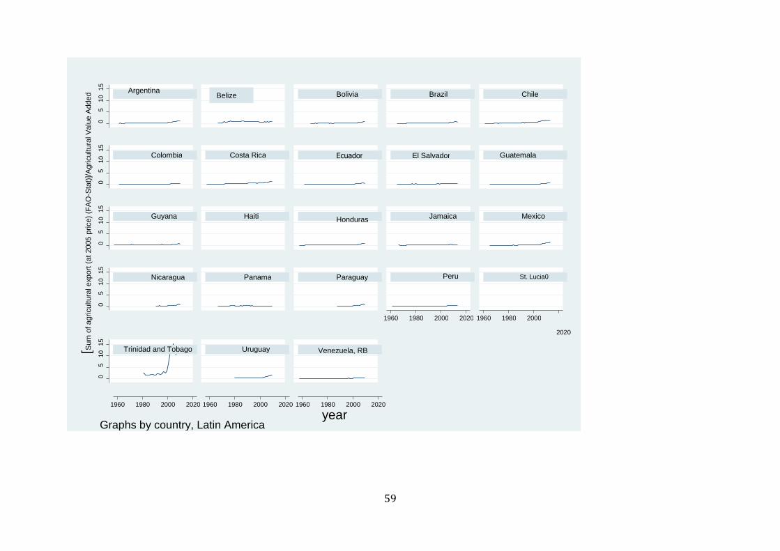
59
0
5
10 1
5
0
5
10 1
5
0
5
10 1
5
0
5
10 1
5
0
5
10 1
5
1960 1980 2000 2020 1960 1980 2000
2020
1960 1980 2000 2020 1960 1980 2000 2020 1960 1980 2000 2020
Argentina Belize Bolivia Brazil Chile
Colombia Costa Rica Ecuador El Salvador Guatemala
Guyana Haiti
Haiti Honduras Jamaica Mexico
Nicaragua Panama Paraguay Peru St. Lucia0
Trinidad and Tobago Uruguay Venezuela, RB [Sum
of agricultura
l export
(at
2005 p
rice)
(FA
O-S
tat)
]/A
gricultura
l V
alu
e A
dded
year Graphs by country, Latin America

60
Top Related