


Languages
Pages
Legal

Santiago de Chile November 14-18 2016
Proximal and remote sensing synergies for monitoring and modelling key vegetation biophysical variables in tree-grass ecosystems: a study case in central Spain
M. Pilar Martín Environmental remote sensing and spectroscopy laboratory (SpecLab)
Spanish National Research Council (CSIC)

Santiago de Chile November 14-18 2016
Monitoring Terrestrial Carbon fluxes
NEP quantification a key issue to improve our understanding of the feedbacks between the terrestrial biosphere and the atmosphere
Re = Ra + Rh NPP = GPP - Ra NEP = GPP – Re
NEP = -NEE
CO2 sinks
Photosynthesis GPP
CO2 sources
Respiration Ra
Respiration Rh
From El Niño and a record CO2 rise Richard A. Betts,Chris D. Jones,Jeff R. Knight,Ralph F. Keeling& John J. Kennedy Nature Climate Change 6, 806–810 (2016)
Observed and forecast CO2 concentrations at Mauna Loa

Santiago de Chile November 14-18 2016
Eddy covariance systems
Eddy covariance (EC) flux towers have been providing continuous measurement of ecosystem level water and carbon exchanges since the early 1990s
https://fluxnet.ornl.gov

Santiago de Chile November 14-18 2016
EC measurements need to be scaled up
The restricted spatial representativeness of EC fluxes measured at site level has limited the scope of the studies based on this data
Wang, H., Jia, G., Zhang, A., & Miao, C. (2016). Assessment of Spatial Representativeness of Eddy Covariance Flux Data from Flux Tower to Regional Grid. Remote Sensing, 8
• Small footprint (< 1 km) • Network of Towers is Discrete in Space

Santiago de Chile November 14-18 2016
Remote sensing: a tool to monitor land parameters
Remote Sensing is an important data source to quantify canopy structure and ecosystem function and phenology
Reflectance can be converted into biophysically meaningful descriptors of the ecosystem: LAI, fCover, fPAR, LST, CWC, biomass, albedo..
Some of these variables are being systematically monitored at coarse spatial resolution by global remote sensing programs
Spatial mismatch between EC measurements and coarser grid-cell of satellite information
Lack of accuracy in complex ecosystems
Santiago de Chile November 14-18 2016
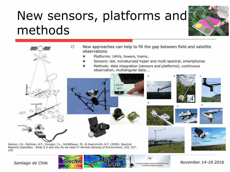
New sensors, platforms and methods
New approaches can help to fill the gap between field and satellite observations
Platforms: UAVs, towers, trams…
Sensors: led, miniaturized hyper and multi spectral, smartphones
Methods: data integration (sensors and platforms), continuous observation, multiangular data….
Gamon, J.A., Rahman, A.F., Dungan, J.L., Schildhauer, M., & Huemmrich, K.F. (2006). Spectral Network (SpecNet) - What is it and why do we need it? Remote Sensing of Environment, 103, 227-235

Santiago de Chile November 14-18 2016
Field (“real”) data
Characterize the site at different scales: from plot to ecosystem
Link the information with EC measurements and other field sensors
Link the information with spectral measurements: ground, airborne and satellite to… Calibrate/validate empirical models
Parameterize/validate radiative transfer models
Validate standard RS products
Spectral calibration of remotely sensed data acquired from UAV/airborne and satellite platforms.
Develop spectral library: spectral characterization of vegetation targets (spatial and temporal dimensions)
Link the information with EC measurements and other field sensors
Link the information with biophysical parameters
Calibrate/validate empirical models
Parametrize/validate radiative transfer models
Integration and upscaling
“Collecting real data gives you insights on what is important and provides necessary information to parameterize and validate models. You must get your boots dirty” (D. Baldocchi, UCB)
Biophysical parameters Spectral data

Santiago de Chile November 14-18 2016
BIOSPEC National funded
project: Ministry of Science and Innovation
2009-2012
FLUXPEC National funded project:
Ministry of Economy and competitiveness
2013-2016
Par
tner
s K
ey
coll
abo
rato
rs
SynerTGE National funded
project: Ministry of Economy and competitiveness
2016-2018

Santiago de Chile November 14-18 2016
BIOSPEC- FLUχPEC: Structure and objectives
WP 1 WP 2
WP 3
WP 4
WP 5
WP 6
Data acquisition
Modelling
Validation
Improvement of remote sensing products to estimate vegetation biophysical parameters and water and carbon fluxes in tree-grass ecosystem
Integration of multi-source proximal and remote sensing data: optical, thermal, LiDAR
To establish relationships between multi-scale spectral data, the estimation of relevant vegetation parameters and the Earth-atmosphere fluxes (EC towers) using empirical as well as physical based models (RTM)
To assess the capacity of proximal and remote sensing to track the dynamics of vegetation and EC fluxes at different temporal scales: daily, seasonally and inter-annually

Santiago de Chile November 14-18 2016
Site general description
Ecosystem: dehesa Mediterranean Holm Oak open woodland (Savanna)
Mediterranean Climate: annual T = 16.7 ºC, annual Prec = 700 mm LAI = 0.4 (trees) + 1-1.5 (grass)
Soil: Stagnic Alisols, depth > 2m. Texture: sandy loam. soil C is 8.5 g/kg and soil N is 0.82 g/kg (0-20cm layer).
Tree canopy: 98% Quercus Ilex; 25 tree/ha; mean DBH = 45cm; canopy height = 7-10 m; canopy fraction = 10-20%
Management: tree pruning every 25 years to optimize acorn production
Herbaceous layer: high biodiversity (easy to find > 20 species within 4 m2); different composition below tree / open;
Management: continuous grazing (cows)
Las Majadas del Tietar (39°56‘29'' N, 5°46'24'’ W), Extremadura, Spain
Santiago de Chile November 14-18 2016
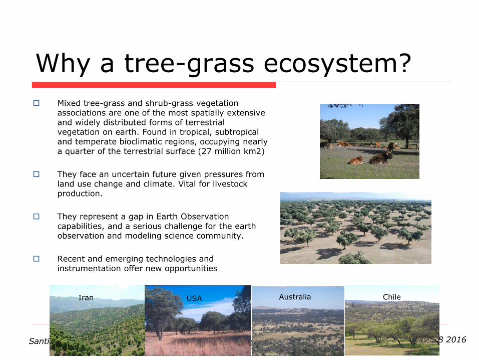
Why a tree-grass ecosystem?
Mixed tree-grass and shrub-grass vegetation associations are one of the most spatially extensive and widely distributed forms of terrestrial vegetation on earth. Found in tropical, subtropical and temperate bioclimatic regions, occupying nearly a quarter of the terrestrial surface (27 million km2)
They face an uncertain future given pressures from land use change and climate. Vital for livestock production.
They represent a gap in Earth Observation capabilities, and a serious challenge for the earth observation and modeling science community.
Recent and emerging technologies and instrumentation offer new opportunities
Iran USA Australia Chile

Santiago de Chile November 14-18 2016
a beautiful ecosystem…
…but also a well stablished experimental site
El-Madany, T., 2016
… and why Majadas?
Santiago de Chile November 14-18 2016
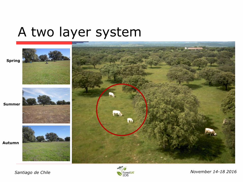
A two layer system
Ecosystem reacts to water availability and demand
Perez-Priego et al. 2016
Spring
Summer
Autumn
2010 2011 2012 2014 2015
Pacheco-Labrador, J. 2016

Santiago de Chile November 14-18 2016
A two dimensional analysis
Temporal: to capture main phenological periods in each stratum but also daily and intra-daily variations (CWC,LUE).
Spatial: different spatial scales need to be considered: sub-plot - plot – pixel - footprint - ecosystem
Sub-plot
plot
Footprint/ecosystem

Santiago de Chile November 14-18 2016
Field data: Temporal dimension
Seasonal and inter-anual
Veg-bio: Regular destructive sampling campaigns (50 from 2009 to 2016)
Field spectroscopy campaigns (ASD Fieldspec 3 VIS-NIR-SWIR)
EC data
Daily and intra-daily
Continuous multiangular hyperespectral system (AMSPEC-MED) 2013-2015
EC data

Santiago de Chile November 14-18 2016
Field data: Spatial dimension
Different spatial scales
Logistic limitations
Grass
25x25 m plots (established location since 2009)
Started with 40 (upper left image)
11 Biospec-Fluxpec plots (yellow boxes)
4 plots North T + 4 plots South T (red boxes).
Trees Started with 10 trees
5 Fluxpec trees (2 Biospec/Fluxpec + 3 Fluxpec) (red dots)
Santiago de Chile November 14-18 2016
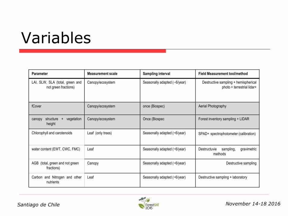
Variables
Parameter Measurement scale Sampling interval Field Measurement tool/method
LAI, SLW, SLA (total, green and
not green fractions) Canopy/ecosystem Seasonally adapted (~6/year) Destructive sampling + hemispherical
photo + terrestrial lidar+
fCover Canopy/ecosystem once (Biospec) Aerial Photography
canopy structure + vegetation
height Canopy/ecosystem Once (Biospec Forest inventory sampling + LIDAR
Chlorophyll and carotenoids Leaf (only trees) Seasonally adapted (~6/year) SPAD+ spectrophotometer (calibration)
water content (EWT, CWC, FMC) Leaf Seasonally adapted (~6/year) Destructuvie sampling, gravimetric
methods
AGB (total, green and not green
fractions)
Canopy Seasonally adapted (~6/year) Destructive sampling
Carbon and Nitrogen and other
nutrients Leaf Seasonally adapted (~6/year) Destructive sampling + laboratory

Santiago de Chile November 14-18 2016
Biophysical and spectral data allows to monitor seasonal dynamics
Green LAI grass
SLA trees current yr
AGB grass
EWT trees current yr

Santiago de Chile November 14-18 2016
Estimation of vegetation biophysical parameters using field spectroscopy (VIS-NIR-SWIR)
Water content grasslands: empirical vs RTMs, canopy
Nitrogen content trees: empirical, leaf

Santiago de Chile November 14-18 2016
Estimation of vegetation biophysical parameters using field spectroscopy (VIS-NIR-SWIR)
Non-parametric linear: Partial Least Squares Regression (PLSR)
Non-parametric non-linear: Random Forest Regression (RFR)
Vilar et al. 2016
Santiago de Chile November 14-18 2016
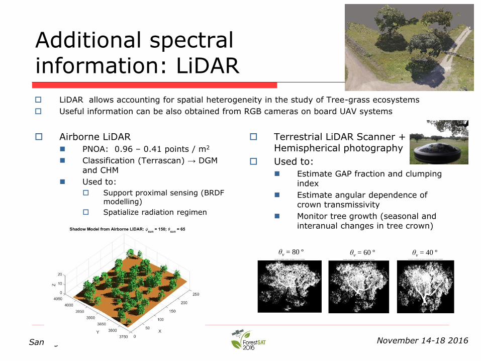
Additional spectral information: LiDAR
Airborne LiDAR
PNOA: 0.96 – 0.41 points / m2
Classification (Terrascan) → DGM and CHM
Used to:
Support proximal sensing (BRDF modelling)
Spatialize radiation regimen
Terrestrial LiDAR Scanner + Hemispherical photography
Used to:
Estimate GAP fraction and clumping index
Estimate angular dependence of crown transmissivity
Monitor tree growth (seasonal and interanual changes in tree crown)
LiDAR allows accounting for spatial heterogeneity in the study of Tree-grass ecosystems
Useful information can be also obtained from RGB cameras on board UAV systems
θv = 80 º θv = 60 º θv = 40 º

Santiago de Chile November 14-18 2016
Continuous multi-angular hyperspectral measurements: AMSPEC-MED
Based on AMSPEC II system Hilker et al., 2010
Unispec DC spectroradiometer (400-1500 nm) + PTU (Azimuth: 20º - 330º / Zenith: 40º – 69º)
Objectives Provide spectral information
Continuous
Directionally corrected
Spectrally unmixed
Relate with Veg. biophysical parameters
Light use efficiency
Other remote observations
Acquisition period August 2013 – March 2016
Santiago de Chile November 14-18 2016
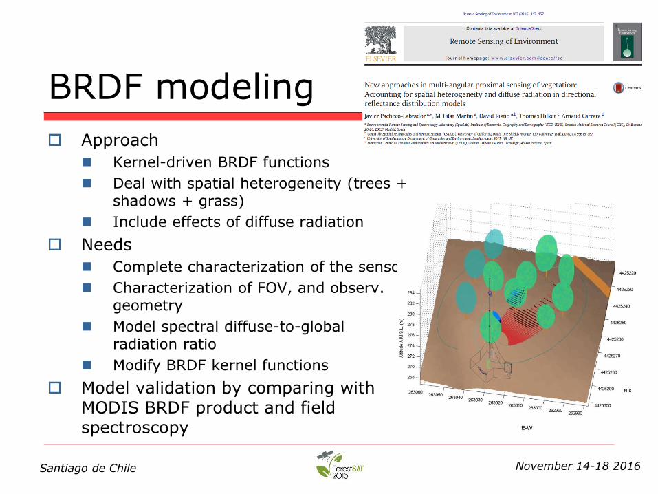
BRDF modeling
Approach
Kernel-driven BRDF functions
Deal with spatial heterogeneity (trees + shadows + grass)
Include effects of diffuse radiation
Needs
Complete characterization of the sensor
Characterization of FOV, and observ. geometry
Model spectral diffuse-to-global radiation ratio
Modify BRDF kernel functions
Model validation by comparing with MODIS BRDF product and field spectroscopy

Santiago de Chile November 14-18 2016
From plot to ecosystem: Airborne hyperspectral images
6 campaings from 2010 to 2016: spring-summer
max. of 8 overpasess/campaign
Different configurations
Spatial overlap (BRDF and LST)
AHS
CASI
CASI AHS
(VSWIR) AHS
(Thermal)
Bands 144 63 17
FWHM (nm)
5.0 18 - 90 300-450
SSI (nm) 4.75 ~ ~
Pixel Size (m)
1.1x1.7 4.8x4.8 4.8x4.8

Santiago de Chile November 14-18 2016
Mapping biofisical parameters (grass layer) Vegetation indices
Regression analysis
Modeling GPP Images -> geocorrected
HDRF (ATCOR + Empirical Line)
Classification
(Mahalanobis):Grass / Trees and Shadows+Water / Roads+Soil
NDVI ~ fPAR
PRI ~ ε (carefully)
From plot to ecosystem: Airborne hyperspectral images
Variable Model R2 RRMSE (%)
FMC -117,833+1027,038*SAVI 0,875 15,2
CWC -0,013+0,0306*MSR 0,843 25,1
LAI -1,218+4,675*NDVI 0,752 28,8
Cm 0,016+(-0,014)*NDVI 0,637 23,4
AGB -0,005+0,025*NDVI 0,702 28,8
Melendo, J.R. 2015

Santiago de Chile November 14-18 2016
Field data is a must!!! necessary information to understand the ecosystem and parameterize and validate models Difficulties to properly characterize the ecosystem at different spatial scales
Difficulties to get spectral data at the crow level: tower based systems and UAVs are a promising alternative
Field protocols adapted to tree-grass ecosystems are needed
Automated tower-based multiangular hyperspectral systems dedicated to detailed study of vegetation properties and status is feasible in heterogeneous ecosystems. However, a detailed characterization of the system optics and observation geometry is required – LiDAR key complementary data
Empirical models outperformed those using RTM in the estimation of biophysical parameters. RTM models need to be adapted (plant species and ecosystem variability!!!)
Left: Apparently homogenous grass cover (plot). Right: Very heterogeneous at sub-plot scale
Leassons learned

Santiago de Chile November 14-18 2016
The magic words
Integration
Data
Methods
Expertise
Networking
Sharing information
Metadata vs standarization

Santiago de Chile November 14-18 2016
Research collaborations at Majadas site
A large scale nutrition manipulation experiment in a tree grass ecosystem to understand ecosystem-physiological response to changing N/P stoichiometry and water availability
Dr. Rasmus Fensholt. Dept. of Geosciences and Natural Resource Management, University of Copenhagen. Denmark
Dr. John Gajardo. Centro de Geomatica, Universidad de Talca. Chile
Dr. Dennis Baldocchi. Biometeorology Lab. University of California Berkeley. USA
Dr. Marta Yebra. Fenner School of Environment and Society. Australian National University. Australia

Santiago de Chile November 14-18 2016
THANKS FOR YOUR ATTENTION!
http://www.lineas.cchs.csic.es/synertge/
http://www.lineas.cchs.csic.es/biospec/
http://www.lineas.cchs.csic.es/fluxpec/
Top Related