


Languages
Pages
Legal


MECH5500-01
MECHANICAL DESIGN PROJECT
Summer 2016
Mr. Anthony Duva
Associate Professor
Department of Mechanical Engineering and Technology
Wentworth Institute of Technology
550 Huntington Avenue
Boston, MA 02115
Professor Duva,
This report contains the entire structure of our team’s process and execution of tasks to conduct
“Performance Analysis and Testing on Wentworth Institute of Technology’s Mini Jet Turbine” in
the thermodynamics laboratory. The report focuses on first upgrading the current instrumentation
and data acquisition (DAQ) system. The new DAQ system directly outputs data recorded by the
mini turbine into a user-friendly LabVIEW interface. Steps were taken in order to accurately
measure the five stages of pressure and temperature of the system, RPM, thrust, and fuel pressure.
These values are paralleled by an EES turbine system analysis, which will be used to calculate the
compressor, turbine, and overall efficiencies, including the overall work of the system.
The existing laboratory experiment report was modified and a new draft was created for future
students to use in their thermodynamics laboratory period. This draft will be under review by
department faculty for finalization. This system gives students the ability to further understand the
first and second laws of thermodynamics in a practical and industry-like setting. A main focus of
this project was to create a friendly user interface for future students running this machine. When
the students are conducting the experiment, the LabVIEW program will acquire run data and
display real time temperature, pressure, RPM, and thrust outputs. These values will be inputted
into the EES program to calculate the actual efficiencies of the system on that given run day.
The tasks that have been completed are as follows: various preparations for DAQ replacement,
pressure transducer and thermocouple implementation and calibration, RPM and thrust calibration,
mounting of laptop arm, laptop and second monitor, mounting of DAQ bracket and DAQs to the
bracket, rewiring of system to new DAQs, a LabVIEW DAQ and technical display program, an
EES program with interactive display, a laboratory experiment, detailed engineering notebooks,
and this final report.
We look forward to your review of the final report,
Sincerely,
Matthew Dietter, Kyle Lavoie, Jonathan Sewell, and Kurtis Madden

Performance Analysis and Testing of
the Mini Gas Turbine
WENTWORTH INSTITUTE OF TECHNOLOGY
MECH5500
Mechanical Capstone Project
Submitted to:
Professor Anthony W. Duva
Date: 8/9/2016
By: Matt Dietter, Kyle Lavoie, Kurtis Madden, Jonathan Sewell
[email protected], [email protected], [email protected], [email protected]
550 Huntington Avenue, Boston, MA 02115

1. ABSTRACT
This report defines the Performance Analysis and Testing of the Mini Gas Turbine that our team
completed for our mechanical engineering capstone project. The main objective of this project was
to restore the capability of the Turbine Engine located in Wentworth Institute of Technology’s
Thermodynamics Laboratory in order to provide a laboratory experiment for future students. This
objective was met through updating the existing data acquisition system, writing a new data
acquisition program in LabVIEW, installing new pressure and temperature sensors, and
performing a first and second law of thermodynamics analysis on the engine in Engineering
Equation Solver. In order to update the existing data acquisition system, new NI SCB-68 connector
blocks were implemented along with NI USB-6251 terminals. The new hardware is operated
through a LabVIEW program running on a new laptop designated and mounted to the mini jet
turbine housing.
Tasks completed in order to finalize this project include formal proposal report, various
preparation for DAQ replacement, pressure transducer and thermocouple implementation and
calibration, mounting of laptop arm, laptop and second monitor, mounting of the DAQ bracket and
DAQs to the bracket, rewiring of system to new DAQs, a LabVIEW DAQ and technical display
program, an EES program with interactive display, a laboratory experiment, detailed engineering
notebooks from each group member, and this final report.
As a result, the mini jet turbine system is now capable of producing consistent run data in order to
be used as an experimental laboratory for future thermodynamic students. Each component of the
system is calibrated including all thermocouples and pressure transducers, RPM, and thrust.
Students will now utilize run data displayed on the LabVIEW front panel and input it into the EES
program to determine various efficiencies and work of the mini turbine system.

Contents
1. ABSTRACT ........................................................................................................................................................ 3
2. PROBLEM DEFINITION ................................................................................................................................ 6
3. INTRODUCTION .............................................................................................................................................. 6
4. PROJECT OBJECTIVE ................................................................................................................................. 10
4.1. DETAILED PERFORMANCE SPECIFICATION ................................................................................................ 10
5. PROJECT PLAN ............................................................................................................................................. 11
6. RESULTS ......................................................................................................................................................... 14
6.1. SYSTEM UPDATES ..................................................................................................................................... 14 6.1.1. Computer System ................................................................................................................................. 14 6.1.2. Hardware Mounting ............................................................................................................................ 16 6.1.3. New Instrumentation ............................................................................................................................ 17
6.2. DATA ACQUISITION ................................................................................................................................... 19 6.2.1. DAQ Hardware .................................................................................................................................... 19 6.2.2. Instrumentation Calibration ................................................................................................................ 22 6.2.3. LabVIEW Software .............................................................................................................................. 29
6.3. ENGINE TESTING ....................................................................................................................................... 35 6.4. ENGINEERING EQUATION SOLVER (EES) .................................................................................................. 41 6.5. THERMODYNAMICS LABORATORY EXPERIMENT ....................................................................................... 47
7. CONCLUSION................................................................................................................................................. 48
8. REFERENCES ................................................................................................................................................. 48
9. APPENDIX ....................................................................................................................................................... 49
9.1. APPENDIX A – TEAM CONTRACT .............................................................................................................. 49 9.2. APPENDIX B – TEAM MEMBER RESUMES .................................................................................................. 50 9.3. APPENDIX C – SAMPLE OF ENGINE TESTING DATA ................................................................................... 54 9.4. APPENDIX D – REVISED THERMODYNAMICS LABORATORY EXPERIMENT ................................................ 55
LIST OF FIGURES
Figure 1. Basic Brayton Cycle ................................................................................................... 7 Figure 2. Turbine Engine Layout (Brayton Cycle) .................................................................... 8 Figure 3. Engine Instrumentation Locations .............................................................................. 9
Figure 4. Project Gantt Chart ................................................................................................... 12 Figure 5. Computer Mount Design ......................................................................................... 14
Figure 6. Laptop and Monitor Installed ................................................................................... 15 Figure 7. Chassis Cover Panel ................................................................................................. 15 Figure 8. Old DAQ Setup ........................................................................................................ 16 Figure 9. New DAQ Design..................................................................................................... 16 Figure 10. DAQ Components Installed ................................................................................... 17
Figure 11. Inlet Pitot Tube Current Set-Up ............................................................................. 17 Figure 12: PX139 Pressure Transducer ................................................................................... 18 Figure 13. Thermocouple Types .............................................................................................. 18
Figure 14: NI USB-6251 (left) and NI SCB-68 (right)............................................................ 19

5
Figure 15: SCB-68 Printed Circuit Board Diagram ................................................................. 20
Figure 16. New Thrust Display ................................................................................................ 21 Figure 17. Initial RPM Calibration Curve ............................................................................... 23 Figure 18. Manual RPM Calibration ....................................................................................... 23
Figure 19. Thrust Calibration Curve ........................................................................................ 24 Figure 20. Thrust Calibration Method ..................................................................................... 24 Figure 21. Compressor Inlet Static Pressure Calibration ......................................................... 25 Figure 22. Pressure Sensor Calibration Method ...................................................................... 25 Figure 23. Compressor Inlet Pressure (P1) Calibration Curve ................................................ 26
Figure 24. Compressor Exit Pressure (P2) Calibration Curve ................................................. 26 Figure 25. Turbine Inlet Pressure (P3) Calibration Curve ....................................................... 27 Figure 26. Turbine Exit Pressure (P4) Calibration Curve ........................................................ 27 Figure 27. Exhaust Gas Pressure (P5) Calibration Curve ........................................................ 28
Figure 28. Compressor Inlet Static Pressure Calibration Curve .............................................. 28 Figure 29. Mass Flow Rate Calibration ................................................................................... 29
Figure 30. Fuel Flow Rate Calibration Curve .......................................................................... 29 Figure 31. LabVIEW Data Acquisition Front Panel User Interface (Main Tab) ..................... 31
Figure 32. LabVIEW Data Acquisition Front Panel User Interface (Plot Tab) ....................... 32 Figure 33. LabVIEW Block Diagram ...................................................................................... 33 Figure 34. Engine Testing Data Plot – Thrust vs RPM ........................................................... 37
Figure 35. Engine Testing Data Plot – Temperature vs RPM ................................................. 38 Figure 36. Engine Testing Data Plot – Inlet Mass Flow Rate vs RPM ................................... 39
Figure 37. Engine Testing Data Plot – Pressure vs RPM ....................................................... 40 Figure 38. EES Formatted Equations - Enthalpy and Entropy ................................................ 42 Figure 39. EES Formatted Equations - Efficiency................................................................... 43
Figure 40. EES Formatted Equations - Thrust ......................................................................... 44
Figure 41. EES Code................................................................................................................ 45 Figure 42. EES Diagram Window ........................................................................................... 46
LIST OF TABLES
Table 1. Engine Manufacturer Specifications .......................................................................... 10 Table 2. New System with Signal Conditioning Parameters ................................................... 19
Table 3. Instrumentation Parameters and Calibration.............................................................. 22 Table 4. Engine Testing Data Sample...................................................................................... 54

2. PROBLEM DEFINITION
The Turbine Technologies Mini Gas Turbine in the Wentworth Institute of Technology
thermodynamics lab is in great need of an instrumentation overhaul. Due to the high cost of
replacing the data acquisition system completely, our team will be replacing it ourselves. The
current DAQ system is outdated and incompatible with current software on the computer it is
paired to. A new set of DAQ hardware will be paired with a new computer running a LabVIEW
program to collect the data.
Our team’s goals also include calibration of pressure transducers and thermocouples for accurate
measurement. Our team will then run a 1st and 2nd law of thermodynamics on the system using
Engineering Equation Solver (EES).
The mini gas turbine in the thermodynamics lab is a fantastic resource that is going un-used. Many
students can benefit from the mini turbine’s technical sophistication. Benefits include but are not
limited to technical understanding, conceptual understanding, and practical application. With the
recent creation of the Aerospace Engineering Minor at Wentworth, this machine could open the
eyes to many young engineers and give them the ability to have a future in the aerospace industry.
Turbine propulsion is used on various aircraft, but dominates the commercial jet and military jet
industries.
The main problem of this project is to overhaul the instrumentation of the mini gas turbine and
have it ready to be run for students in the upcoming fall of 2016 semester. Instrumentation, testing,
and calibration are the three main milestones for this project. A technical lab will be produced for
thermodynamics students to run.
3. INTRODUCTION
The turbine engine discussed throughout this report is a self-contained turbojet engine that is used
as an educational tool for engineering students. This engine operates on a Brayton cycle. The
Brayton cycle depicts the air-standard model of a gas turbine power cycle. A simple gas turbine is
comprised of three main components: a compressor, a combustor, and a turbine. According to the
principle of the Brayton cycle, air is compressed in the compressor. The air is then mixed with
fuel, and burned under constant pressure conditions in the combustor. The resulting hot gas is
allowed to expand through a turbine to perform work. Most of the work produced in the turbine is
used to run the compressor and the rest is available to run auxiliary equipment and produce power.
The gas turbine is used in a wide range of applications. Common uses include stationary power
generation plants (electric utilities) and mobile power generation engines (ships and aircraft). In
power plant applications, the power output of the turbine is used to provide shaft power to drive a
generator, a helicopter rotor, etc. A jet engine powered aircraft is propelled by the reaction thrust
of the exiting gas stream. The turbine provides just enough power to drive the compressor and
produce the auxiliary power. The gas stream acquires more energy in the cycle than is needed to
drive the compressor. The remaining available energy is used to propel the aircraft forward.

7
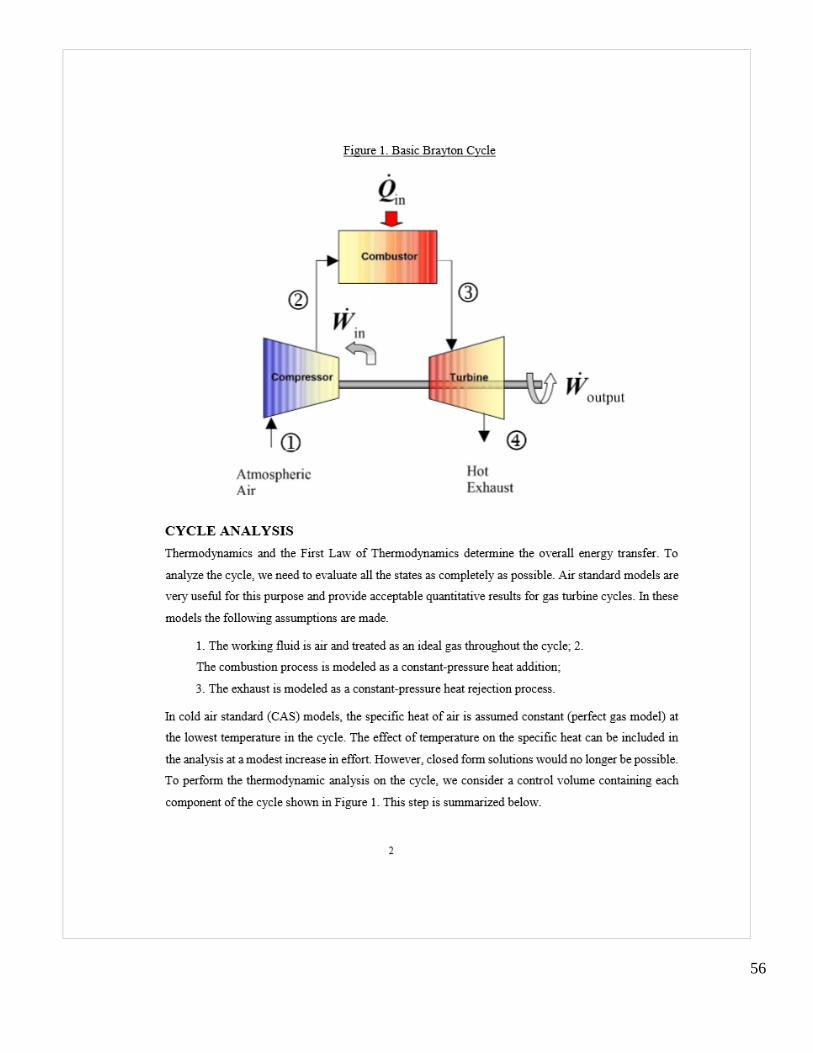
Shown below in Figure 1 is a schematic of the Brayton cycle. Low-pressure air is drawn into a
compressor (state 1) where it is compressed to a higher pressure (state 2). Fuel is added to the
compressed air and the mixture is burnt in a combustion chamber. The resulting hot gases enter
the turbine (state 3) and expand to state 4.
Figure 1. Basic Brayton Cycle
An analysis on this engine provides important performance characteristics such as thrust,
compressor performance, turbine performance (work and power, expansion ratio, turbine
efficiency), combustion/emission analysis, and overall isentropic efficiency. In order to perform
an analysis on this engine, several quantities at specific locations are needed. Sensors are
instrumented on this engine at the compressor inlet, compressor outlet, turbine inlet, turbine exit,
and exhaust to collect data on the temperature and pressure at each location. This data is then used
to perform a performance analysis on the engine. In addition, there are sensors on this engine to
monitor thrust, RPM, and fuel flow rate.

Shown below in Figure 2 is a cross section of the engine with main components labeled.
Figure 2. Turbine Engine Layout (Brayton Cycle)

9
Figure 3 below shows the location of each temperature and pressure being measured on the engine.
Figure 3. Engine Instrumentation Locations

Shown below in Table 1 are the specifications of the engine.
Table 1. Engine Manufacturer Specifications
Manufacturer Turbine Technologies, Ltd.
Model Number 2000DX
Max. RPM 90,000
Max. Exhaust Temperature 720 C
Pressure Ratio 3.4:1
Specific Fuel Consumption 1.18 lb./lb.-hr
4. PROJECT OBJECTIVE
The objectives of this capstone project are as follows:
1. Replace existing DAQ components with new NI DAQ
2. Rewire the DAQ components to generate temperature, pressure, RPM, and thrust outputs
3. Create mounting bracket for new DAQ components
4. Generate LabVIEW program to output data from new DAQ
5. Calculate first and second law of thermodynamics analysis on components and the
overall system to find overall efficiencies using Engineering Equation Solver
6. Develop a project to be conducted by future thermodynamics students
4.1. Detailed Performance Specification
By utilizing the previously attached instrumentation, the majority of the form, fit, and function of
the design has already been established. The main components that will be added are as follows:
New LabVIEW program with user friendly interface
New computer and computer mount
Shelving unit to hold the NI chassis
Measurement device to read inlet air velocity
Collectively these items will revamp and improve the preexisting DAQ system. The laptop and
stand will be placed on the right side of the unit in order for easy access to connect to the NI
chassis. Above the laptop there will be a second screen mounted for a user friendly display of the
EES program or LabVIEW front panel. The shelving unit will be mounted inside the unit to allow
the chassis to be mounted and for the instrumentation to be easily connects. A measurement device
for reading inlet air velocity will be added in for proper analysis.
In addition to the instrumentation and components for the DAQ system, an EES program using
first and second law analysis will be created. This will allow for comparison between calculated
and measured results.
The outcomes for this project will be a laboratory report for student use, our final report, and our
final poster presentation. Throughout the semester there will be formal and information
PowerPoint presentations, informing the other teams in our course section. This will improve our

11
presentation skills, our ability to convey technical information and to solve problem and innovate
through group discussion.
5. PROJECT PLAN
The responsible parties of this senior capstone project are Matthew Dietter, Kyle Lavoie, Jonathan
Sewell, and Kurtis Madden. Our mentors throughout the semester will be Professor Anthony Duva
and Professor Haifa El-Sadi of the Mechanical Engineering & Technology department at
Wentworth.
Our team’s qualifications are primarily from major/minor courses along with work experience. Each
of the group members is majoring in mechanical engineering and minoring in aerospace engineering
which has given a wide range of courses that apply directly to this project. Resumes of each team
member are attached in Appendix B.
Due to the location of the mini gas turbine in the thermodynamics lab, the vast majority of our
meetings and working sessions will and have occurred there.
This project will be graded on the ability for this system to be used by students as a laboratory
experiment. This goal entails that the DAQ system is fully functional and outputting data correctly,
the turbine system is calibrated and producing repeatable data, and there is a tangible laboratory
experiment ready for student use.
The work plan process we have used has been consistent from the start of this project. Our team
created a Microsoft Project file and have been revising it consistently with respect to our current
and projected timelines. Professor Duva has been mentored us on how a realistic timeline functions
and how to estimate lead times for various tasks.
The Gantt chart for this capstone project has been an ever-changing reference, updated at nearly
every meeting to correspond with the current timeline of our capstone project. Below in Figure 4 is
our final detailed Gantt chart.

Figure 4. Project Gantt Chart

The following is a description of the budget for this project. Purchased parts for revamping the
DAQ system will be the primary cost during this project. The LabVIEW and EES software is
provided so there will be no additional cost for software. The budget breakdown is as follows:
1 Lenovo T440p computer - $1595
1 computer stand - $55
2 National Instrument SB-68 - $341 each
2 National Instrument USB-6251 - $2,053 each
1 12” x 24” steel sheet metal - $30
Miscellaneous, i.e. wiring, adhesives… - $100
According to the items listed above, the total budget for this project is $6718. Labor will be
performed by all group members and Wentworth faculty, therefore there will not be any additional
cost for work done. Consultation with Professor Duva and Professor El-Sadi will also not incur
any additional cost. Altogether, the budget will be fully funded by the Mechanical Department of
Wentworth Institute of Technology.
The future of this project’s successful completion includes the use of the fully functional turbine
engine as a thermodynamics laboratory experiment for mechanical engineering students. Future
students will be able to run the engine and collect data in order to calculate the efficiency of the
engine. In addition, the EES program will provide students a secondary tool to perform an analysis
on the engine. A goal of this project is to be able to obtain consistent results.

6. RESULTS
This section outlines system updates including a new computer system, new hardware mounting
system, new instrumentation, data acquisition hardware, instrumentation calibration, LabVIEW
software, engine testing overview and experimental data, and Engineering Equation Solver (EES)
analysis.
6.1. System Updates
System updates include a new computer system, new hardware mounting system, select new
instrumentation.
6.1.1. Computer System
One of the first updates was mounting the new laptop and monitor securely to the system. It was
important that they were mounted rigidly and looked professional since this is a direct user to
system interface. A laptop mount was purchased which came with an adjustable arm and mounting
bracket. Since the sheet metal housing for the engine is not very rigid, a thicker mounting block
was made to strengthen the mount. Figure 5 below shows the design of the mount. Figure 6 below
shows the entire system mounted and installed.
Figure 5. Computer Mount Design

15
Figure 6 below shows the laptop system mounted and installed.
Figure 6. Laptop and Monitor Installed
Lastly, a panel was made to cover the opening where the access to the old DAQ was. This was
simply a piece of aluminum sheet metal cut to size and painted to match the rest of the sheet metal
housing. Figure 7 below shows the cover panel installed on the system.
Figure 7. Chassis Cover Panel

16
6.1.2. Hardware Mounting
Removing all of the old DAQ components and mounting the new DAQ was another major task in
the system update. Since the new DAQ has several additional components which are much larger
than the old system a much larger mounting bracket was necessary. After modeling all of the
current system components in SolidWorks, a sheet metal bracket was designed to fit all of the
DAQ components without interfering with any of the existing surrounding components. Figure 8
below shows the old DAQ setup.
Figure 8. Old DAQ Setup
Figure 9 below shows the design of the new DAQ setup.
Figure 9. New DAQ Design

17
Figure 10 below shows the final mounting of the new DAQ system.
Figure 10. DAQ Components Installed
6.1.3. New Instrumentation
During the course of this project, there were many sensors that needed to be changed or added.
The preexisting DAQ system was capable of collecting temperature and pressure readings from
the various mini-turbine engine stages; however, there was room for improvement. One of the
main additions made to the instrumentation was implementing a new pressure transducer to read
the static pressure at the inlet of the nozzle. The pitot-static mast style device can be seen below in
Figure 11:
Figure 11. Inlet Pitot Tube Current Set-Up
The preexisting set-up had both the dynamic and static pitot lines attaching to the P1 pressure
transducer. This allowed for the correct differential pressure to read; however, velocity could not
be calculated due to the unknown density. By being able to read the static pressure, correct velocity

18
can be calculated using the know density at the static pressure and Bernoulli’s equation. In order
to get the correct static pressure reading from the preexisting set-up, the static tube was to be teed
off and attached to a PX139 pressure transducer. The other port on the PX139 was be left open to
the atmospheric air within the housing. Below in Figure 12, the new transducer and set-up can be
seen:
Figure 12: PX139 Pressure Transducer
In addition to a new pressure transducer, three thermocouples had to be replaced. Part of the
process of implementing the new DAQ system was to test each instrumentation component
individually to ensure they were functioning properly. When testing thermocouples T3 (Turbine
Inlet), T4 (Turbine Exit), and T5 (Exhaust Gas) there was significant noise experienced. After
isolating each thermocouple from the engine and ruling out broken wires as the cause, it was
determined that the noise was a result of ground loops and crosstalk. To relegate this issue, various
grounding methods, including sheath grounding, were tested without success. It was ultimately
decided that the thermocouples experiencing the issue needed to be replaced completely with a
different type. The three main types of thermocouples can be seen below:
Figure 13. Thermocouple Types

19
The three thermocouples which had been experiencing the grounding issues were determine to be
of the grounded type. The grounded type has its wire touching the sheath which is what resulted
in the ground loops and electrical noise. To fix the noise issue, the turbine inlet (T3) thermocouple
and the turbine exit (T4) thermocouple were replaced with an ungrounded type of the same size.
The exhaust gas temperature thermocouple was also replaced. The thermocouple selected was an
exposed type which responds quickly (EGT is a critical temperature) and does not experience
electrical noise. The specifications for the new thermocouples are as follows:
Table 2. New System with Signal Conditioning Parameters
6.2. Data Acquisition
Data acquisition includes DAQ hardware description, instrumentation calibration, and LabVIEW
software description.
6.2.1. DAQ Hardware
The basis of this project is to transition from the outdated TBX-68T and old software which is no
longer supported, to the new hardware and supported LabVIEW software. The hardware chosen
for the task are the NI SCB-68 and NI USB-6251. Two of each have been implemented in the
DAQ system.
Figure 14: NI USB-6251 (left) and NI SCB-68 (right)
Thermocouple
LocationStyle Connector Calibration Sheath
Length
(in)
Diameter
(in)Junction Omega Model
T3 - Turbine Inlet
Temperature
Quick
DisconnectStandard K SS 12 0.125 Ungrounded KQSS-18U-12
T4 - Turbine Exit
Temperature
Quick
DisconnectMini K SS 12 0.125 Ungrounded KMQSS-125U-12
T5 - Exhaust Gas
Temperature
Quick
DisconnectMini K SS 6 0.125 Exposed KMQSS-125E-6

20
One NI SCB-68 and NI USB-6251 will be dedicated to thermocouple temperature readings, and
the other to pressure transducer readings and other voltage readings. The NI SCB-68 allows for
single-ended and differential temperature measurements to be made. For the temperature readings
to be made, the differential temperature mode will be used as it is more accurate than single-ended.
In order to perform this, the SCB-68 needs to be configured for temperature reference to be enabled
within LabVIEW. This will allow for the built-in Cold Junction Compensation of the SCB-68 to
be utilized. The built-in Cold Junction Compensation temperature sensor can be seen below in as
well as AI channels to be utilized can be seen in Figure 15 below.
Figure 15: SCB-68 Printed Circuit Board Diagram
For measurements using pressure transducers and other instrumentation, the SCB-68 will be in
the factory default setting for correct voltage readings. The PX139 pressure transducer will be
attached to the built-in +5V power supply within the SCB-68. The instrumentation that will also
be attached to this chasses consist of the RPM and thrust indicators. Each of the SCB-68 has 8
different AI channels that can be used for instrumentation; between the two a total of 16 devices
can be connected.
While attempting to calibrate the thrust strain gauge, significant noise to the NI chassis was
experienced. The pre-existing set-up had the wires from the strain gauge splitting between the
meter and the NI chassis. While the out-put signal from the strain gage was filtered through the
DP25-S, it was not filter through the NI chassis. To remedy the issue, the DP25-S was replaced

21
with a DP25-S-A which had the correct analog signal output. With the new signal analog signal
output, there was no noise experienced from the thrust strain gage and meter. Below the new meter
can be seen:
Figure 16. New Thrust Display

6.2.2. Instrumentation Calibration
The instrumentation on the turbine engine, including new sensors, are shown below in Table 3.
Also listed in Table 3 are the signal conditioning parameters and calibration curves for each sensor.
New sensors, or replaced sensors, from the existing instrumentation list contain a new sensor part
number in the Measurement Type column.
Table 3. Instrumentation Parameters and Calibration
AI Name Measurement Type Range Calibration m Calibration b
NI SCB-68 Module 2
0 Compressor
Inlet Press VDC 0-1 PSIG 67.183 0
1 Compressor
Exit Press VDC 0-6 PSIG 1016 -0.9964
2 Turbine Inlet
Press VDC 0-6 PSIG 1000 0
3 Turbine Exit
Press VDC 0-5 PSIG 101.4 -0.06873
4 Nozzle Exit
Pressure VDC 0-5 PSIG 101.4 -0.06894
5
Compressor
Inlet Static
Pressure
VDC (Omega
PX139-0.3D4V
2G18-21)
0-0.3 PSIG 0.1504 -0.3515
6 Fuel Flow VDC 0-5
GAL/Hr 83.33 0
NI SCB-68 Module 1
1 Compressor
Inlet Temp K type 0-2000 ˚C
2 Compressor
Outlet Temp K type 0-2000 ˚C
3 Turbine Inlet
Temp
K type (Omega
KQSS-18U-12) 0-1000 ˚C
4 Turbine Exit
Temp
K type (Omega
KMQSS-125U-12) 0-1000 ˚C
5 Exhaust Gas
Temp
K type (Omega
KMQSS-125E-6) 0-1000 ˚C
6 Thrust VDC 0-25 Lbs 12.135 -24
7 RPM* VDC 9.484E4-
2.720E-1 258226 38687
* Further scaling performed – see RPM calibration below
Thermocouples
Thermocouples do not have custom scaling curves; they are configured within the data acquisition
board (NI SCB-68) as well as within the LabVIEW DAQ Assistant. For correct temperature
readings, “Temperature Sensor Enabled” has to be set on the SCB-68 and the Cold Junction

23
Compensation has to be set to “Built-In” in LabVIEW. In addition, within LabVIEW, the
thermocouple setup is set to type K.
RPM
Shown below in Figure 17 is the initial RPM calibration curve. This calibration curve is not
necessary, but it was set when further calibration was performed – it does not affect the accuracy
in any way, but it must be included in the DAQ Assistant prior to further calibration.
Figure 17. Initial RPM Calibration Curve
The RPM module outputs the RPM on a frequency domain rather than a voltage signal. The
frequency of the signal is measured in LabVIEW and is manually scaled to correspond with the
actual RPM. This calibration curve consists of a slope (m) of 62.65 and a Y-intercept (b) of
negative 671.25.
Figure 18. Manual RPM Calibration

24
Thrust
The calibration curve for the thrust measurement is shown below in Figure 19. This calibration
curve was obtained through pull-testing the engine with a scale and determining the corresponding
voltage output. The thrust display was calibrated using the device manual which will be contained
within a package of this report.
Figure 19. Thrust Calibration Curve
Figure 20. Thrust Calibration Method
Pressure Sensors
All pressure calibration curves remained the same from the existing DAQ system except for the
Compressor Inlet Static Pressure and Compressor Inlet Dynamic Pressure sensors. The
Compressor Inlet Static Pressure needed calibration because it was a completely new sensor to the

25
system. In addition, the Compressor Inlet Dynamic Pressure transducer needed calibration because
the static pressure was connected into the same hose coming out of the pitot static tube as the
Dynamic pressure sensor.
The pressure sensors that were calibrated, were done so using a Pasco Heat Engine. The calibration
method includes applying a force on the top of the piston (known weights), calculating the
theoretical pressure, and reading the voltage output from the pressure transducer. The relationship
between pressure and voltage can then be obtained through a linear trend line. This calibration was
verified using a manometer at atmospheric pressure. An example of the Compressor Inlet Static
Pressure calibration curve plot is shown below in Figure 21.
Figure 21. Compressor Inlet Static Pressure Calibration
The Pasco Heat Engine is shown below in Figure 22.
Figure 22. Pressure Sensor Calibration Method
y = 0.1504x - 0.3515
R² = 0.9995
0.000
0.050
0.100
0.150
0.200
0.250
0.300
0.350
2.7 2.9 3.1 3.3 3.5 3.7 3.9 4.1 4.3 4.5
Pre
ssure
(p
si)
Voltage
Compressor Inlet Static Pressure Calibration - Pressure
vs Voltage

26
Shown below in Figure 23 through Figure 28 are calibration curves for all main pressure sensors.
Figure 23. Compressor Inlet Pressure (P1) Calibration Curve
Figure 24. Compressor Exit Pressure (P2) Calibration Curve

27
Figure 25. Turbine Inlet Pressure (P3) Calibration Curve
Figure 26. Turbine Exit Pressure (P4) Calibration Curve

28
Figure 27. Exhaust Gas Pressure (P5) Calibration Curve
Inlet Mass Flow Rate
Figure 28. Compressor Inlet Static Pressure Calibration Curve
In order to calculate the Inlet Mass Flow Rate to the turbine engine, the static pressure is needed.
The static pressure is obtained by connecting a pressure transducer directly to the static pressure
port on the inlet pitot tube. Next, the density of the air is calculated using this static pressure. The

29
air velocity is calculated next using the Dynamic Pressure which is the difference between the total
pressure and the static pressure. The Mass Flow Rate is finally obtained knowing the density,
velocity and cross sectional area of the inlet nozzle at the location of the pitot tube. This calculation
is performed in the LabVIEW program (Figure 29). See following report section for mass flow
rate governing equations.
Figure 29. Mass Flow Rate Calibration
The fuel flow rate is determined from measuring the fuel pressure. If the fuel pressure as well as
the fuel properties are known, the flow rate can be determined. The fuel flow rate calibration curve
is shown below in Figure 30.
Figure 30. Fuel Flow Rate Calibration Curve
6.2.3. LabVIEW Software
Acquiring data from the new instrumentation system on the turbine engine is performed through a
LabVIEW program. LabVIEW is installed on the new computer that has been installed onto the
engine system. Users of this program will easily be able to acquire all necessary data in order to
perform a thermodynamic analysis on the engine.

30
The user interface of the LabVIEW program includes a front panel that contains two main
interfaces – the “Main” tab which includes numerical values for each sensor on the engine as well
as a diagram indicating the location of each sensor, and a “Plot” tab which includes a graph in
which the user can determine what quantities are plotted.
This program is installed onto the lab computer as an executable application. The result of this is
such that the code controlling the program cannot be modified directly. If changes are needed in
the program, the original source code will need to be modified and a new application will need to
be created. This is done through the VI – “Tools” > “Build Application (EXE) From VI”.
When the program is opened, live data values will begin displaying on all indicators and graphs.
It is important to note, that due to the nature of the RPM sensor it will not read an accurate value
until the engine beings spinning at several hundred RPM. This can be tested through the air start
on the engine chassis.
An option is available to toggle data collection on and off. The default value is off. First, a filename
and save location need to be inputted. Next, the “Collect Data” option will need to be pressed to
begin data collection and data collection will end once it is disabled. The next time the “Collect
Data” toggle is enabled, if the user does not update the filename, a new filename will be created
with a sequential number added to the end. This will help avoid overwriting existing data files
created by the user.

Figure 31 below shows the LabView main tab layout of the DAQ display.
Figure 31. LabVIEW Data Acquisition Front Panel User Interface (Main Tab)

32
Figure 32 belows shows the LabView plot tab layout of the DAQ display.
Figure 32. LabVIEW Data Acquisition Front Panel User Interface (Plot Tab)

33
Figure 33. LabVIEW Block Diagram

Shown above in Figure 33 is the LabVIEW program block diagram. The structure of the program
is such that the code is all contained within a while loop. The while loop will run the code until a
condition is met. The condition is true until the “Stop” button on the front panel is pressed, sending
a false Boolean signal to the case structure. The following sections describe the corresponding red
labels on the above figure.
1. The data is acquired through the LabVIEW Express functions, DAQ Assistant. There are
two DAQ Assistant functions, each corresponding to the two NI SCB-68’s. Within the
DAQ Assistant, signal parameters are set such as Number of Samples, Sampling Rate,
Terminal Configuration, Scaling, and Acquisition Mode. In order to simplify further signal
processing, both DAQ Assistants are set to 1000 Samples to Read at a rate of 10,000 Hz
with an Acquisition Mode set to “N Samples”. All temperature channels are set to degrees
Fahrenheit, Thermocouple Type K, with a Built-In CJC Source. All remaining channels
are set to Differential Terminal Configuration with the correct Custom Scaling option
selected.
2. After the signal leaves the DAQ Assistant, they are averaged using the Express Statistics
function. The number of samples that are averaged together correspond to the number of
Samples to Read which is set in the DAQ Assistant to be 1000 samples. The arithmetic
mean is outputted from the function. Averaging a large sample set helps to remove noise
from the signal.
3. The signal leaving the Express Statistics function is a 1D array of Dynamic Data Type
Signals. A “Split Signals” function is used to separate the Dynamic signals from the 1D
array. The corresponding signals are then brought to their numeric indicators for display
on the front panel.
4. All signals, except for RPM, are voltage signals that are scaled to the correct dimension.
The RPM signal is a frequency not a voltage. Because of this, further processing of the
signal is needed. An Express Select Signals function is used to index the RPM signal from
the 1D array of Dynamic signals. The RPM signal is then brought to an Express Tone
Measurements function where the frequency of the signal is determined. Through manual
calibration, a scale was determined. The frequency output from the Tone Measurements
function is then manually scaled to the correct value corresponding to the RPM of the
engine. The result is then connected to the RPM numeric indicator for display on the front
panel.
5. The Inlet Mass Flow Rate numeric indicator value is calculated, not measured. The
calculated value is dependent on the measured values of Compressor Inlet Temperature
(T1), Compressor Inlet Static Pressure (Ps), and Compressor Inlet Dynamic Pressure (Pt-
Ps). Using Express Formula functions, the density of the air is first calculated, then the
velocity of the air is calculated, and finally the Inlet Mass Flow Rate can be calculated. The
following equations are contained within these functions for Density (ρ), Velocity (v) and
Mass Flow Rate (ṁ).

35
𝜌 =(𝑃𝑠 + 14.7)144
𝑅(𝑇1 + 460) (𝑠𝑙𝑢𝑔/𝑓𝑡3)
𝑣 = √2𝑃1 ∗ 144
𝜌 (𝑓𝑡/𝑠)
�̇� = 𝜌𝐴𝑣 (𝑠𝑙𝑢𝑔/𝑠) Where,
A = Compressor Inlet Area
R = Ideal Gas Constant for Air
6. The data leaving the numeric indicators is put back into a 1D array using the Merge Signals
function. The merged signal is then brought to a Waveform Chart function to be displayed
on the front panel Plot Data tab. The plot on this tab contains an interactive legend in which
values can be toggled on or off to be displayed.
7. The same set of merged signals that is going to the Main Plot is also brought to the Express
Write to Measurement File function. A file extension is added to the filename string and
then concatenated with the Save Location string in order to be valid for the Filename input
on the Write to Measurement File function. The Collect Data toggle switch is wired to the
Enable input on the Write to Measurement File function.
8. The date and time displayed on the front panel are obtained through the Get Date/Get Time
function. A Time Delay function is implemented to control how fast the while loop iterates.
This controls how fast values are updated on the front panel. The Time Delay is set to 0.10
Seconds.
6.3. Engine Testing
In order to validate the new DAQ hardware, sensors, and software, the Turbine Engine has gone
through several test runs. The following steps illustrate the operating procedure for the Turbine
Engine.
1. Prior to engine start-up, ensure the following:
a. Air compressor is plugged in (located behind engine) and the air compressor
pressure gage reads 100 psi or greater.
b. There is a sufficient amount of fuel in the tank – use dipstick to get fuel level.
c. The air exhaust vent is running.
2. Rotate key to on position.
3. Turn electrical master toggle switch to on position.
4. Position throttle handle at approximately 50%.
5. Turn ignition toggle switch to on position.
6. Turn air toggle switch to on position and wait until RPM indicator displays
approximately 10,000 to 13,000 RPM.
7. Turn fuel toggle switch to on position.

36
a. If Exhaust Gas Temperature does not begin to increase after approximately 3
seconds, increase throttle position to approximately 60-75%. If Exhaust Gas
Temperature still does not begin to increase after approximately 1-2 seconds, turn
fuel toggle switch to off position along with the ignition and air toggle switches.
Wait for unburned fuel to dry from engine. Consult lab technician for further
instructions.
8. Once engine is running, turn air and ignition toggle switches to off position.
9. Back throttle positon off so that the engine idles at approximately 48,000 to 50,000 RPM.
NOTE: Try to keep idle rpm above 48,000 minimum. If hang flame appears behind the exhaust,
bring throttle down and then push back up in order to suck flame away.
To spin down and turn off:
1. Position throttle all the way down.
2. Turn the fuel toggle switch to off position.
3. As engine is spinning down, turn the air switch on momentarily to help cool.
A sample set of data collected from an engine test run is shown in Appendix C at the end of this
report. This same data is represented below in Figure 34 through Figure 37. These plots contain
important characteristics of the engine such as the relationship between engine RPM and Thrust,
Temperature, Inlet Mass Flow Rate, and Pressure.

Figure 34. Engine Testing Data Plot – Thrust vs RPM
0
5
10
15
20
25
30
35
45000 50000 55000 60000 65000 70000 75000 80000
Thru
st (
lbf)
RPM
Thrust vs RPM

38
Figure 35. Engine Testing Data Plot – Temperature vs RPM
0
200
400
600
800
1000
1200
1400
45000 50000 55000 60000 65000 70000 75000 80000
Tem
per
ature
(F
)
RPM
Temperature vs RPM
Compressor Inlet Temperature (T1) Compressor Exit Temperature (T2)
Turbine Inlet Temperature (T3) Turbine Exit Temperature (T4)
Exhaust Gas Temperature (T5)

39
Figure 36. Engine Testing Data Plot – Inlet Mass Flow Rate vs RPM
0
0.005
0.01
0.015
0.02
0.025
45000 50000 55000 60000 65000 70000 75000 80000
Mas
s F
low
Rat
e (S
lug/s
)
RPM
Inlet Mass Flow Rate vs RPM

40
Figure 37. Engine Testing Data Plot – Pressure vs RPM
0
5
10
15
20
25
30
45000 50000 55000 60000 65000 70000 75000 80000
Pre
ssure
(psi
g)
RPM
Pressure vs RPM
Compressor Inlet Pressure (P1) Compressor Exit Pressure (P2) Turbine Inlet Pressure (P3)
Turbine Exit Pressure (P4) Exhaust Gas Pressure (P5)

6.4. Engineering Equation Solver (EES)
One of the critical tasks was to create a program in EES which analyzes the engine using the first
and second laws of thermodynamics. Ideally this program would be displayed on the second
monitor so you can take the data directly from LabView and plug it into the EES program. After
plugging in the different temperatures and pressures as inputs in the EES program, it will calculate
the compressor efficiency, turbine efficiency, overall efficiency of the engine and the thrust of the
engine. These values can be calculated using each set of data output from LabView. Since the
engine has a large range in RPM, the ranges in efficiencies can be seen as the engine accelerates
and decelerates. A diagram window interface was created in EES to make it easy for the user to
run the program without understanding the entirety of the code. Figure 41 below shows the
equations window section of the EES program. Figure 42 below shows the diagram window
section of the EES program.

42
Shown below in the following set of EES formatted equations are fluid property calculations in
order to obtain enthalpy and entropy values at locations throughout the engine cycle. These values
are obtained through the built in EES thermo-physical property calculator.
Figure 38. EES Formatted Equations - Enthalpy and Entropy

43
Shown below in Figure 39 are EES formatted equations that calculate work and efficiency for the
turbine, compressor, and of the engine overall. These calculations utilize enthalpy and entropy
values obtained in the above set of formatted equations.
Figure 39. EES Formatted Equations - Efficiency

44
Shown below in Figure 40 are calculations involved in calculating the thrust of the engine. In order
to calculate the thrust, the inlet velocity and exit velocity of the air through the engine is calculated
through continuity equation as well as Bernoulli’s equation assuming incompressible flow.
Figure 40. EES Formatted Equations - Thrust

Figure 41. EES Code

Figure 42. EES Diagram Window

6.5. Thermodynamics Laboratory Experiment
Engineering Thermodynamics II Project Draft
While redeveloping the mini-turbine DAQ system, a new project for Engineering
Thermodynamics II students was created. The current document is still in its draft stage and under
review for implementation. The ultimate goal of the semester long project is for students to develop
an understanding of a standard Brayton Cycle. The initial objective of the project is for students to
successfully run and collect data from the mini-turbine. Upon retrieving data, the students are then
to analyze the results and calculate various properties of the mini-turbine. Through the use of EES,
students are expected to create their own program which will solve for efficiencies and work of
the different components and overall engine.
Revised Mini-Turbine Lab
After updating the pre-existing DAQ system and implementing a new LabVIEW program, the lab
instructions needed to be updated. Revisions to the old lab consisted mainly of updates to the
experimental procedure which went through the steps of starting the engine and recording data.
The new LabVIEW program required a new procedure in which a file name and location is set
before a data collection toggle switch is turned on. In addition to the new collection process, the
user can also view plots of the data on another tab. Aside from the implementation of the new
DAQ instructions, the overall lab remained the same. This revised lab is contained within
Appendix D.

7. CONCLUSION
The completion of our capstone project produced quality and timely task completion. The mini
turbine engine is now ready to be used in student experimental settings. Each data acquisition
component of the system is calibrated including all thermocouples and pressure transducers, RPM
measurement and thrust measurement. The LabVIEW program will be used for real time data
display and data acquisition of the complete run cycle of the system. Using this data exported to
Excel by the LabVIEW program, these values can be inputted into the first and second law of
thermodynamics EES program to determine the efficiencies of the compressor, turbine, and the
overall system as well as the work done by the system in BTU/hr.
Many tasks and sub-tasks have been completed leading us to our final goal. These tasks and sub-
tasks include but are not limited to preliminary research and component identification, mounting
of a new laptop arm and laptop, design and manufacturing of a mounting bracket for the DAQ
hardware, an up to date Microsoft project file, a completed formal proposal report, an EES
program, a DAQ and user-friendly display LabVIEW program, a thermodynamics laboratory
report, our engineering notebooks, and this final report.
8. REFERENCES
[1] Moran, Michael J., and Howard N. Shapiro. Fundamentals of Engineering
Thermodynamics.Seventh ed. New York: Wiley, 2011. Print
[2] Klein, S. A.. Engineering Equation Solver for Microsoft Windows Operating Systems. F-
ChartSoftware. 2014
[3] National Instruments. SCB-68 User Manual. National Instruments Corporation. Austin,
Texas.2009.
[4] National Instruments. USB-6251 User Manual. National Instruments Corporation. Austin,
TX.2008.
[5] Omega. Thermocouple Selection Guide. Omega Engineering Inc.. Stamford, CT. 2016
[6] Omega. PX139 Series Pressure Sensor User Guide. Omega Engineering Inc.. Stamford,
CT.2008

9. APPENDIX
9.1. Appendix A – Team Contract
Team Contract As a member of team number 1, I agree that coordinated teamwork is essential for successfully completing assigned
projects. I understand my individual performance will affect the success of the entire project. I also understand that
all members of successful teams need to exhibit the following behaviors during the execution of the project:
1. Fulfills duties of team role
a. Attend all team meetings
b. Actively participate in team meetings
c. Be prepared to present work assigned from previous meeting
2. Researches and gathers pertinent information
3. Listens to other teammates
4. Shares work evenly
5. Regularly scheduled meetings will meet:
a. Time/Day:10/Wed Place: Class
b. Time/Day:11/Wed Place: Meeting w/Professor
c. Time/Day: 12/Mon Place: 610 make shift library
Printed Team Member Name Team Member Signature
1. Matt Dietter
2. Jon Sewell
3. Kurt Madden
4. Kyle Lavoie

50
9.2. Appendix B – Team Member Resumes

51

52

53

9.3. Appendix C – Sample of Engine Testing Data
Table 4. Engine Testing Data Sample
Full engine testing data set contained within report package.

9.4. Appendix D – Revised Thermodynamics Laboratory Experiment
56

57

58

59

60

61

62

63

64

65

66
Top Related