


Languages
Pages
Legal


MACRO-FINANCIAL INTERACTIONS
IN A CHANGING WORLD2020
Eddie Gerba and Danilo Leiva-Leon
Documentos de Trabajo
N.º 2018

MACRO-FINANCIAL INTERACTIONS IN A CHANGING WORLD
Documentos de Trabajo. N.º 2018
2020
(*) We would like to thank the participants of the 2019 Bayesian Econometrics Workshop, 34th Annual Congress of the European Economic Association, 50th Annual Conference of the Money, Macro and Finance Research (LSE), and the Research Seminar Series of the Danmarks Nationalbank, and two referees from its working paper series, for helpful comments and suggestions. The views expressed in this paper are those of the authors. No responsibility for them should be attributed to the Banco de España, the Eurosystem or the Danmarks Nationalbank.(**) Danmarks Nationalbank, Havnegade 5, 1093 Kobenhavn, DK. E-mail: [email protected].(***) Banco de España, Alcalá 48, 28014 Madrid, SP. E-mail: [email protected].
Eddie Gerba (**)
DANMARKS NATIONALBANK
Danilo Leiva-Leon (***)
BANCO DE ESPAÑA
MACRO-FINANCIAL INTERACTIONS IN A CHANGING WORLD (*)

The Working Paper Series seeks to disseminate original research in economics and fi nance. All papers have been anonymously refereed. By publishing these papers, the Banco de España aims to contribute to economic analysis and, in particular, to knowledge of the Spanish economy and its international environment.
The opinions and analyses in the Working Paper Series are the responsibility of the authors and, therefore, do not necessarily coincide with those of the Banco de España or the Eurosystem.
The Banco de España disseminates its main reports and most of its publications via the Internet at the following website: http://www.bde.es.
Reproduction for educational and non-commercial purposes is permitted provided that the source is acknowledged.
© BANCO DE ESPAÑA, Madrid, 2020
ISSN: 1579-8666 (on line)

Abstract
We measure the time-varying strength of macro-fi nancial linkages within and across the
US and euro area economies by employing a large set of information for each region. In
doing so, we rely on factor models with drifting parameters where real and fi nancial cycles
are extracted, and shocks are identifi ed via sign and exclusion restrictions. The main
results show that the euro area is disproportionately more sensitive to shocks in the US
macroeconomy and fi nancial sector, resulting in an asymmetric cross-border spillover
pattern between the two economies. Moreover, while macro-fi nancial interactions have
steadily increased in the euro area since the late 1980s, they have oscillated in the US,
exhibiting very long cycles of macro-fi nancial interdependence.
Keywords: macro-fi nancial linkages, dynamic factor models, TVP-VAR.
JEL classifi cation: E44, C32, C55, F44, E32, F41.

Resumen
En este trabajo se estudia la evolución del grado de interconexiones macrofi nancieras,
tanto dentro de las economías de Estados Unidos y de la zona del euro como entre
ellas. Para esto, el estudio se basa en modelos de factores dinámicos con parámetros
cambiantes en el tiempo, los cuales se utilizan para extraer ciclos reales y fi nancieros de
un gran conjunto de información asociado a cada región. En estos modelos, las
perturbaciones reales y fi nancieras correspondientes son identifi cadas mediante
restricciones de signo y exclusión. Los principales resultados muestran que la zona
del euro es desproporcionadamente más sensible a las perturbaciones en el sector
fi nanciero y macroeconómico de Estados Unidos, lo que da como resultado un patrón
de contagio transfronterizo asimétrico entre las dos economías. Además, si bien las
interacciones macrofi nancieras han aumentado constantemente en la zona del euro
desde fi nales de los años ochenta, estas han oscilado en Estados Unidos, exhibiendo
ciclos muy amplios de interdependencia macrofi nanciera.
Palabras clave: interconexiones macrofi nancieras, modelo de factores dinámicos,
vectores autorregresivos.
Códigos JEL: E44, C32, C55, F44, E32, F41.

BANCO DE ESPAÑA 7 DOCUMENTO DE TRABAJO N.º 2018
1 Introduction
The eagerness to understand macro-financial linkages has been brisk and unprecedented
over the recent years. Much of this has been driven by the desire to comprehend the
forces that lead to the Great Recession, including the deep and long-lasting consequences
from the financial downturn that began in 2007. In particular, recent research on macro-
finance has focused on the role of the financial sector as a generator of shocks, which are
transferred to the overall economy via macro-financial linkages. Less (albeit some) effort
has been put in understanding how the macroeconomy can create and transmit shocks
to the financial sector. Moreover, very little effort has been invested in grasping the role
that linkages themselves may play as amplifier and feedback loop for shocks generated
inside the linkages as well as elsewhere. Yet, the prospect for a full recovery seems bleach
at present. Despite unprecedented monetary expansion and supportive fiscal policy, per-
capita income growth has stagnated in many jurisdictions, including the US and euro
area. Therefore, understanding how macro-financial interactions can condition a potential
recovery has become crucial for policy makers.
Figure 1 shows a diagram that illustrates the complexities embedded in macro-financial
interactions. Each economy in the figure has two sectors, macroeconomic and financial.
Domestic spillovers between the sectors in the US (euro area) are denoted by red (blue)
solid arrows. In parallel, cross-border interactions between the sectors are denoted with
dashed arrows. Moreover, all these relationships may be subject to potential fundamental
changes over time due to a number of reasons, opening an additional dimension to the
problem. One outcome from Figure 1 is that the study of international macro-financial
dynamic interactions, albeit crucial for policy makers, is challenging due to all the possible
ways in which shocks could be transmitted. The aim of this paper is to provide a robust
assessment of these interactions by taking into account all these underlying dimensions.
The first part of the problem involves defining what the macroeconomic and financial
cycles are. Yet, in the empirical literature there is still a wide debate on the exact defini-
tion of a real cycle and how different and more complete it is from the standard business
cycle. For the financial counterpart, there is even less consensus on what constitutes a
financial cycle, its statistical characterization, and how similar it is to the real cycle. The
existing definitions, usually, tend to be narrow (normally incorporating just a few variables
in order to capture the multi-faceted nature of the real or financial sectors), exogenously

BANCO DE ESPAÑA 8 DOCUMENTO DE TRABAJO N.º 2018
1Section 2 provides a detailed review of the literature on the study of macro-financial linkages.
Figure 1: International Macro-Financial Dynamic Interactions
United States Euro Area
Financial
Macro
Financial
Macro
Note: Solid red (blue) arrows denote the domestic macro-financial interactions forthe US (euro area). Dashed red arrows make reference to the spillovers from the USto the euro area. Dashed blue arrows denote the spillovers from the euro area to theUS
pre-determined (constructed such that they reproduce pre-determined statistical charac-
teristics), or based on short time series samples.1
Recognising the above short-comings, this paper attempts to provide a comprehensive
definition of real and financial cycles using dynamic factor models. Unlike previous studies,
our empirical framework allows for an endogenous and time-varying selection of variables in
the construction of each of the latent cycles, selecting from a large dataset of real activity
and financial indicators, for each economy. These variables include information about
output, employment, production, consumption, etc., on the real side, and information
regarding balance sheets, credit, foreign financial activity, etc., on the financial side of the
economy. The motivation for including this feature in our modelling strategy relies on the
need for robustness in the determination of the most relevant variables driving the financial
cycle over time, given the lack of consensus about its definition.
The second part of the problem consists of measuring the intensity of the evolving
macro-financial interactions. To quantify the degree of time variation and profundity in
linkages, the cycles are allowed to endogenously evolve according to a structural VAR model
with drifting coefficients. Also, in order to provide robust assessments, the identification of
real and financial shocks is based on a wide range of schemes that assume exclusion, sign
BANCO DE ESPAÑA 9 DOCUMENTO DE TRABAJO N.º 2018
2*=Transatlantic Trade nd Investment Partnership
and timing restrictions on the impulse response functions. To the best of our knowledge
this is the first study of macro-financial spillovers between the US and the euro area, each
as single economic units, that covers a period starting in the 1980s. In particular, the
sample starts in 1981:II for the case of the euro area, which is considerably longer than
the sample analyzed in any of the previous studies that focus on macro-financial linkages
in this region. Equally, due to good data availability, for the US we can go as far back as
1960:I.
Moreover, we measure the linkages between macroeconomic and financial conditions in
a number of ways in order to provide a comprehensive assessment. Besides the qualitative
comparison of the real and financial cycles, and the computation of their time-varying
correlation, we examine the mutual impact and propagation of structural shocks over time,
calculate the time-varying forecast error variance decomposition at different horizons to
assess the predictive power that one cycle has on another, and examine the time-varying
factor loadings for the real as well as financial cycle to measure the strength of common
patterns inside each sector.
Lastly, the third part of the problem focuses on quantifying the intensity of cross-border
spillovers in the macro-financial sphere. In doing so, we propose a joint (two-economy)
model which basically nests the two single-economy models. Considering that US and the
euro area top the list of global GDP figures, it is of global relevance to understand their
dynamics and cross-border propagation of shocks. Moreover, the topic is of high policy
relevance considering the recent attempts to bring the two economies closer by creating
special economic agreements (such as TTIP*), foster deeper financial cross-border flows
(global banks, EU passport in banking and market financing in euro area), and enforce
regulatory harmonization (transatlantic mutual recognition of regulation in securities and
derivatives, Basel III and FSB).2
With longer and smoother financial cycles compared to the macroeconomic, both in
the euro area and in the US, our results robustly uncover a number of highly policy-
relevant features about the evolution of international macro-financial interactions. First,
while the euro area has exhibited increasing commonalities in the financial sector since
the early 2000s, the strength of commonalities in the US financial sector has remained
relatively steady over time. In particular, euro area private sector liabilities have become
increasingly determinant for the shape and evolution of financial cycles. Second, while in

BANCO DE ESPAÑA 10 DOCUMENTO DE TRABAJO N.º 2018
the euro area, macro-financial interactions have steadily increased since late 1980’s, in the
US, they have oscillated, exhibiting very long cycles of macro-financial interdependence.
Moreover, the integration of the financial sector in the overall economy and the increase in
the interplay between the two sectors has been more intense in the US, while more solid
and gradual in the euro area. Third, we unveil significant differences in the transmission of
mutual shocks. In the euro area, the propagation of shocks has increased in both directions,
that is, from financial to real, and real to financial, but in the US, it has only increased
in the first direction, from financial to real. Likewise, the degree of responsiveness of the
financial sector to macroeconomic shocks is comparatively higher in the US, suggesting
a deeper integration between the two sectors. Fourth, the intensity in transmission of
macro-financial shocks across borders is highly asymmetric, mainly going from US to euro
area. In particular, there is a dimension of asymmetry whereby unexpected deteriorations
in the US economy are detrimental for euro area financial conditions, while, unexpected
deteriorations in the euro area economy could be beneficial for the financial conditions in
the US. These asymmetries increased over time, until the Great Recession.
The rest of the paper is organized as follows. Section 2 provides a brief review of
the literature that helps to identify our contributions. Section 3 describes the employed
empirical framework. Section 4 analyzes domestic macro-financial linkages. Section 5
studies international spillovers. Section 6 concludes.
2 Contacts with the literature
The financial turmoil of 2008 sparked an interest in studying the structural interplay
between financial cycles and the broader economy. While the questions raised in those
studies were not necessarily new, and build on the arguments laid out in the 1930’s and
1970’s (Fisher (1933) and Minsky (1977)), the scope of the pre-Great Recession studies were
much narrower, focusing either on a few cycles, particular aspect, or a particular segment
of the financial sector. For instance, there were studies that showed the procyclical nature
of the financial system (Borio et al. (2001) and Borio and Lowe (2002)). Others have tried
to find long-run regularities in financial crises and the factors leading up to them (Reinhart
and Rogoff (2009)).3
3In a recent work Jorda et al. (2017) document a set of historical features of macro-financial linkages,pointing to the prominent role that financial factors should have in macroeconomic models.

BANCO DE ESPAÑA 11 DOCUMENTO DE TRABAJO N.º 2018
4Moreover, these studies either assume that the frequency between the two types of series is similar, orthat financial is ex ante longer than the business cycle.
5These studies also find that financial cycles, in general, are longer than real cycles, but show evidencefor both short- and medium-term cycles in real credit growth
The recent empirical studies examining the interplay between macroeconomic and fi-
nancial cycles can generally be divided in two main strands. The first one focuses on the
measurement of both cycles, which presents challenges, especially, when defining a financial
cycle. Instead, the second strand focuses on assessing changes over time in the relationship
between macroeconomic and financial cycles. Next, we proceed to briefly review the two
strands of the literature to elucidate the contributions of this paper.
In first place, studies that have focused on the measurement of the cycles can be grouped
into four categories. The first category uses frequency-based filters to extract the cyclical
components of macroeconomic and financial variables, and to describe their similarities
and differences. Most of these studies find that financial cycles are longer in length and
larger in amplitude than business cycles, but with an increasing synchronization over time
(Drehmann et al. (2012), Aikman et al. (2015), Gerba (2015), Schueler et al. (2017) and
Gerba et al. (2017b)). However, since these measures are not based on a given theory or
model, the analysis of their interdependence can return spurious results, as it is shown in
Phillips and Jin (2015).4 This is also the case for the second category, which focuses on
extracting cycles in frequency domain (Strohsal et al. (2015) and Schueller et al. (2017)).5
An important short-coming of this method is that since it requires stationarity, it makes
it difficult to endogenously account for potential structural brakes, which may result in a
lengthening or shortening of the cycles. Third, a less restrictive way of depicting the two
cycles is by relying on turning points identification, by using the Bry-Boschan algorithm
(Harding and Pagan (2002), (2006)).6 The main drawback with this method is that it
is excessively agnostic, and therefore, also has very limited theory to explain the results.
Fourth, to overcome some of the drawbacks of non-parametric or agnostic filters, model-
based filters have been employed. This method is usually based on unobserved component
models used to extract cycles by relying on the Kalman filter (Galati et al. (2016) and
Ruenster and Vlekke (2016)).
In parallel, different empirical strategies have been employed to infer potential changes
in the relationship between macroeconomic and financial variables. The most employed tool
6As show in Claessens et al. (2011) and Drehmann et al. (2012) financial cycles are also found to belonger than business cycles, although Cagliarini and Price (2017) don’t find sufficient evidence. Moreover,they find that business cycles display a higher degree of synchronisation with credit and house price cyclesthan with equity prices.

BANCO DE ESPAÑA 12 DOCUMENTO DE TRABAJO N.º 2018
7Kaufmann and Valderrama (2010) apply a similar framework to also assess the case of the euro area.8In a recent work, Leiva-Leon et al. (2018) evaluate changes in the propagation of shocks between credit
sentiment and the macroeconomy by relying on a multivariate Markov-switching framework.
has been the vector autoregressions (VARs) subject to parameter instabilities. Blake (2000)
and Calza and Sousa (2006) use Threshold VAR models to measure the effect of credit
shocks on real activity, for the US and euro area, respectively. Both studies show evidence
of a stronger impact occurring under low credit growth regimes. For similar purposes,
Davig and Hakkio (2010), Hubrich and Tetlow (2015), and Nason and Tallman (2015) use
Markov-switching VAR models to study the relationship between financial stress and US
economic activity.7 All these studies agree in that the propagation of financial shocks to
the real economy is different during high financial stress regime in comparison to normal
times.8 Other studies allow for instabilities in the VAR models that are smoother than
sudden changes of regimes, that is, by allowing parameters to evolve according to random
walks. For example, Prieto et al. (2016) use a time-varying parameter (TVP) VAR model
to analyze the contribution of credit spread shocks to the US economy. Gambetti and Musso
(2017) follow a similar approach to investigate the effect of credit supply shocks. Ciccarelli
et al. (2016) investigate commonalities and spillovers in macro-financial linkages by using
a panel VAR model with drifting coefficients.9 An important drawback of these studies is
that the employed measure of financial cycles is based on one or a few financial variables,
which usually are related to credit activity only. This is because of the computational
problems arising in estimating such models using a large number of variables. However,
this limitation precludes the estimation of a broad measure of the financial cycle, which is
a crucial feature, given its complexity and lack of consensus about its definition.
The two strands of the literature described above have been somehow disconnected.
This paper intends to unify them by, first, extracting both macroeconomic and financial
cycles from a large set of information with Kalman filtering techniques, and second, casting
those extracted cycles into a structural VAR model with time-varying parameters to assess
changes in the propagation of their shocks. This modelling strategy, which consists of
a joint estimation procedure, described in Section 3 and Appendix A, allows us to infer
changes in macro-financial linkages from a robust and broader perspective than previous
studies. Additionally, we allow for a changing and flexible selection of variables driving
both the financial and real cycle, and identify real and financial shocks with a strategy that
is based on sign, exclusion and timing restrictions on the impulse response functions.
9 Also, Abbate et al. (2016) purse a similar goal, but from an international perspective.
BANCO DE ESPAÑA 13 DOCUMENTO DE TRABAJO N.º 2018
We also incorporate an international dimension to our analysis by looking at cross-
border spillovers between the US and the euro area, both within the sectors, and across.
In this regard, most of the studies have looked at the US outward spillover, finding that
US financial and real shocks matter significantly for the rest of the world. Using a struc-
tural VAR model for pre-2008 data, Bayami and Thahn Bui (2010) find that international
business cycles are largely driven by US financial shocks, with minor role for shocks from
other advanced economies. Miranda-Agrippino and Rey (2018) equally find that there are
large financial spillovers from the US to the rest of the world.
Our framework is more extensive than previous studies since it allows to identify outward
as well as inward spillovers in the US and the euro area, both within the sector as well as
across them. Moreover, we allow the degree of spillover effects between the two regions to
exhibit potential changes over time. Therefore, we provide a full spectrum of international
macro-financial interactions, that is, across regions (US and euro area), across sectors
3 Empirical framework
This section describes the econometric framework used to jointly (i) extract macroeco-
nomic and financial cycles from large datasets and (ii) assess the evolving interdependence
between these cycles. Let Ft be a vector that contains nf indicators of financial conditions
and Rt be a vector containing nr indicators of real activity for a given economy. Our aim
is to provide a framework that allows for a flexible selection of the variables driving both
cycles over time, and that also accounts for potential changes in the propagation of real
and financial shocks.
3.1 One-economy model
We rely on a dynamic factor model with drifting loadings and where the factors evolve
according to a VAR model with time-varying coefficients. Accordingly, consider the model
described in the following equations,
(Macroeconomic and Financial), and over time. The related literature is relatively limited,
and most of related works assess the degree of financial crises spill-overs across markets,
without considering the across sectors aspect (real economy), or the non-crises times.10
10For instance, Gravelle et al. (2006) find evidence of shift-contagion across currency markets, but notbond markets. Dungey et al. (2010) find that the degree of shift-contagion depends on the crisis, withhigher levels during subprime US 2007 crises or the 1998 Russian/LTCM crisis.

BANCO DE ESPAÑA 14 DOCUMENTO DE TRABAJO N.º 2018
11In the empirical applications, we assume k = 2.
⎡⎣ Ft
Rt
⎤⎦ =
⎡⎣ Λf,t 0
0 Λr,t
⎤⎦⎡⎣ ft
rt
⎤⎦+
⎡⎣ vf,t
vr,t
⎤⎦ , (1)
⎡⎣ ft
rt
⎤⎦ = Φ1,t
⎡⎣ ft−1
rt−1
⎤⎦+ · · ·+ Φk,t
⎡⎣ ft−k
rt−k
⎤⎦+
⎡⎣ uf,t
ur,t
⎤⎦ , (2)
where ft and rt denote the financial conditions and real activity factors, respectively.11
The idiosyncratic innovations, vt = (vf,t, vr,t)′, are assumed to be orthogonal between them
and normally distributed, vt ∼ N(0, diag(Ω)). The reduced form innovations from the
VAR, ut = (uf,t, ur,t)′, are also assumed to be normally distributed, ut ∼ N(0,Σ). To be
able to assess the propagation of real and financial shocks, we let ut = A−1εt, where the
vector εt = (εf,t, εr,t)′, denotes the underlying structural shocks, such that E(εtε
’t) = I,
and E(εtε’t−k) = 0, ∀k, and A denotes the impact multiplier matrix.
To allow for changes over time in the information contained in the cycles and in the
propagation of shocks between real and financial cycles, we let both the autoregressive
coefficients φt = vec(Φt), where Φt = [Φ1,t, ...,Φk,t], and the factor loadings λt = vec(Λt),
where Λt = [Λf,t,Λr,t]′, to be time-varying by following random walk dynamics,
φt = φt−1 +wt, (3)
λt = λt−1 + ωt. (4)
The innovations wt and ωt are white noise Gaussian processes with zero mean and constant
covariances, Ψw and Ψω, respectively.
To identify macroeconomic and financial shocks previous studies have mainly relied on
simple recursive, or Cholesky, identification strategy (Davig and Hakkio (2010), Hubrich
and Tetlow (2015), Nason and Tallman (2015), Abbate et al. (2016), Ciccarelli et al. (2016),
Prieto et al (2016)), which can be highly controversial. In a recent work, Gambetti and
Musso (2017) relied on the use of large set of sign restrictions to identify loan supply shocks.
In this paper, we rely on a recent work by Arias et al. (2018) and use a combination of a
few sign, exclusion and timing restrictions to identify macroeconomic and financial shocks.
Additionally, we use an alternative identification strategy as robustness exercise, proposed
by Bai and Wang (2015).

BANCO DE ESPAÑA 15 DOCUMENTO DE TRABAJO N.º 2018
Regarding the strategy based on the combination of restrictions, first, we assume that
real activity and financial conditions are persistent processes by assuming positive signs
in the off-diagonal entries of the impact multiplier matrix, A−1. Second, we assume that
positive real activity shocks have positive contemporaneous effect on financial conditions,
but that a shock in financial conditions does not have a contemporaneous effect on real
activity. As noticed in Prieto et al. (2016) (and many other studies), this assumption im-
plies that macroeconomic variables react with a delay to financial shocks, possibly because
of wealth effects and other effects which involve financial intermediaries that take time to
materialize. In contrast to financial variables, that may react instantaneously to macroe-
conomic shocks. Third, consequently, we assume that it would take at least one period
for real activity to react to a shock in financial conditions. Therefore, we postulate that
a positive unexpected change in the financial cycle positively affects the real cycle with a
one period lag. Although, in the two-economy model, described in the next section, the
restriction on the non-contemporaneous effect of financial on macroeconomic conditions is
relaxed and financial shocks are allowed to contemporaneously influence real activity. The
combination of these restrictions is summarized in Table 1.
Table 1: Sign, Exclusion and Timing Restrictions for the One-economy model
Financial Shock Real Shock
h=0Financial Cycle + +Real Cycle 0 +
h=1Financial Cycle ∗ ∗Real Cycle + ∗
Note: The symbol ∗ indicates that no restriction is imposed inthe corresponding relationship, and “h” denotes the horizon ofthe impulse response.
Bai and Wang (2015) proposed a way to perform structural analysis in a context of
dynamic factor models with factors that are governed by a vector autoregressive structure.
This identification strategy simply consists of directly restricting the variance-covariance
matrix of the reduced form innovations to be an identity matrix, that is, Σ = I. It is
important to notice that, unlike previous studies that measure macro-financial linkages
based on VAR models that contain observed data, our framework relies on a VAR system
that only includes latent variables. This particular feature facilitates the identification of

BANCO DE ESPAÑA 16 DOCUMENTO DE TRABAJO N.º 2018
the underlying macroeconomic and financial shocks. This is because the shocks are jointly
estimated with the rest of the parameters of the model, and by imposing this restriction,
the rest of elements in the model are adjusted in a way that the resulting innovations ut
have a structural interpretation by construction. As a robustness exercise, we alternatively
employ this approach to assess the propagation of shocks between macroeconomic and
financial cycles. This information corresponds to the solid arrows, red for US and blue for
⎡⎢⎢⎢⎢⎢⎢⎣
FUSt
RUSt
FEAt
REAt
⎤⎥⎥⎥⎥⎥⎥⎦
=
⎡⎢⎢⎢⎢⎢⎢⎣
ΛUSf,t 0 0 0
0 ΛUSr,t 0 0
0 0 ΛEAf,t 0
0 0 0 ΛEAr,t
⎤⎥⎥⎥⎥⎥⎥⎦
⎡⎢⎢⎢⎢⎢⎢⎣
fUSt
rUSt
fEAt
rEAt
⎤⎥⎥⎥⎥⎥⎥⎦+
⎡⎢⎢⎢⎢⎢⎢⎣
vUSf,t
vUSr,t
vEAf,t
vEAr,t
⎤⎥⎥⎥⎥⎥⎥⎦
(5)
euro area, in Figure 1. The use of all these alternative identification schemes would allow
us to provide robust assessments on the evolving nature of macro-financial interactions.
3.2 Two-economy model
The factor model described above is estimated for the two economies, US and euro area,
separately in order to provide a deep and accurate understanding of their corresponding
macro-financial linkages. However, we are also interested in identifying potential changes
in the cross-border spillovers between the two economies. In particular, we are interested
in estimating the time-varying effect of (i) financial shocks in the US to the financial cycle
in the euro area, (ii) real shocks in the US to the real cycle in the euro area, (iii) financial
shocks in the US to the real cycle in the euro area, (iv) real shocks in the US to the financial
cycle in the euro area, (v) financial shocks in the euro area to the financial cycle in the US,
(vi) real shocks in the euro area to the real cycle in the US, (vii) financial shocks in the
euro area to the real cycle in the US, and (viii) real shocks in the euro area to the financial
cycle in the US This information corresponds to the dashed arrows in Figure 1, red for
spillovers from US to the euro area, and blue for spillovers from euro area to US.
In order to address these issues, we propose an extended, or joint, model that nests each
of the two models for individual economies. Accordingly, consider the following US-euro
area dynamic factor model:

BANCO DE ESPAÑA 17 DOCUMENTO DE TRABAJO N.º 2018
⎡⎢⎢⎢⎢⎢⎢⎣
fUSt
rUSt
fEAt
rEAt
⎤⎥⎥⎥⎥⎥⎥⎦
= Ψ1,t
⎡⎢⎢⎢⎢⎢⎢⎣
fUSt−1
rUSt−1
fEAt−1
rEAt−1
⎤⎥⎥⎥⎥⎥⎥⎦+ · · ·+Ψk,t
⎡⎢⎢⎢⎢⎢⎢⎣
fUSt−k
rUSt−k
fEAt−k
rEAt−k
⎤⎥⎥⎥⎥⎥⎥⎦+
⎡⎢⎢⎢⎢⎢⎢⎣
uUSr,t
uUSf,t
uEAr,t
uEAf,t
⎤⎥⎥⎥⎥⎥⎥⎦
(6)
where FUSt and RUS
t denote the set of information on financial and real activity, respectively,
for the US economy. Similarly, FEAt and REA
t denote the same set of information but for
the euro area economy. Notice that, consequently, this joint model would extract four
latent factors associated to the financial and real cycles for the US (fUSt and rUS
t ) and for
the euro area (fEAt and rEA
t ). The main advantage of this joint model is that we allow
for the four latent factor to be endogenously interrelated in a VAR fashion. Moreover, we
also allow for time variation in the parameters of the VAR in order to identify changes
in the cross-border propagation of macroeconomic and financial shocks. The dynamics of
the evolving parameters are assumed to be of the same nature as the ones detailed in the
region-specific models, that is, following independent random walks.
The reduced form innovations, u∗t = (uUSr,t , u
USf,t , u
EAr,t , u
EAf,t )
′, and structural innovations,
ε∗t = (εUSr,t , ε
USf,t , ε
EAr,t , ε
EAf,t )
′, are linked through the impact multiplier matrix, that is, u∗t =
B−1ε∗t . The main challenge associated to the joint model arises when defining the restric-
tions to identify cross-border spillovers. As noticed in Prieto et al. (2016), structural
(DSGE) models are still not available in a form to derive meaningful and widely accepted
sign restrictions to disentangle real and financial shocks (see Eickmeier and Ng (2011) for
a discussion). However, we take advantage of the fact that the model incorporates two
economies instead of only one in order to define a set of restrictions that help us to identify
the underlying structural shocks. In particular, we assume that, within each region, there
is a positive and contemporaneous response of real activity and financial conditions to both
real and financial shocks. Next, we assume that euro area developments, in general, have
no contemporaneous impact on US developments, with only one exception. We allow for
the possibility that the financial conditions in the US and euro area contemporaneously
influence each other. Finally, we assume that positive US real shocks are favorable for
both real and financial conditions in the euro area. However, a positive financial shock in
the US would take at least one period to generate a positive influence on the euro area
macroeconomic conditions. This set of restrictions can be summarized in Table 2.

BANCO DE ESPAÑA 18 DOCUMENTO DE TRABAJO N.º 2018
For robustness purposes, we additionally estimate the model by assuming an alterna-
tive shock identification strategy, which consists of a Cholesky factorization in Table 5 of
Appendix A.2. In doing so, we assume the following order of the latent factors. We order
first the US real cycle, followed by the US financial cycle, and by the real cycle of the euro
area, leaving at the end the financial cycle of the euro area. Notice that this order implies
that (i) financial shocks take at least one period to affect macroeconomic conditions, and
(ii) US developments could affect contemporaneously euro area developments, but not vice
versa.
For further validation purposes, we re-estimate the model using a mixture of recursive
and sign-restrictions as outlined in Table 6 of Appendix A.2. It consists of three parts: (i)
recursive restrictions within each block; (ii) euro area shocks do not contemporaneously im-
pact the US; (iii) leave unrestricted the effects that US shocks have on euro area. This is an
alternative scheme that is sufficiently broad to incorporate the empirical results contained
in the current international macro-financial literature.
The overall output retrieved by the models described in this section provides a compre-
hensive analysis of macro-financial interactions along the following dimensions: (i) within
sectors of a given economy (ii) across sectors within a given economy, (iii) across sectors
and across economies, and (iv) over the time dimension. Moreover, we provide a series
of additional exercises for robustness purposes, altering the estimation method of the la-
tent cycles, the identification of structural shocks, and potential changes in the volatility
of macroeconomic and financial cycles. In sum, given the high complexity of measuring
macro-financial linkages at the international level, we adopt a series of alternative exercises
with the only aim of gathering main messages that describe, from a robust and meaningful
way, how macroeconomic and financial shocks propagate across borders.
Table 2: Sign and Exclusion Restrictions for the Two-economy model
Fin. Shock E.A. Real Shock E.A. Fin. Shock US Real Shock US
Financial Cycle E.A. + + ∗ +Real Cycle E.A. + + 0 +Financial Cycle US ∗ 0 + +Real Cycle US 0 0 + +
Note: The symbol ∗ indicates that no restriction is imposed in the corresponding relationship.

BANCO DE ESPAÑA 19 DOCUMENTO DE TRABAJO N.º 2018
4 Macro-financial linkages
This section provides a comprehensive overview of the time-varying interactions between
macroeconomic and financial sectors, for the US and euro area. In doing so, we provide
different pieces of information designed to study these interactions from various perspec-
tives, for each economy separately. First, we assess the evolving strength of commonalities
within each of the two sectors, that is, macroeconomic and financial. This is done by jointly
characterizing the underlying cycles and inferring the segments of the real and financial
sectors that are most important for driving those cycles over time. Second, we provide
a characterization of the joint propagation of macroeconomic and financial shocks. This
is performed by examining the time-varying correlation between the cycles, and analyzing
information contained in impulse responses and forecast error variance decompositions. We
aim to provide a discussion that is comparative in nature, consequently, the description
of the results is structured per type of features, and not per economy. Notice that in
the analysis, we use the terms linkages and interactions interchangeably, treating them as
synonyms for deep and dynamically evolving relations between the two sectors. This is
in contrast to the commonly used word nexus or link that we interpret as not profoundly
changing over time.
4.1 Data
The description of the variables for the US economy is reported in Table 3, and was
retrieved from St. Louis Fed database. The sample spans from 1960:I until 2017:IV,
covering four very distinct episodes in US contemporaneous economic history including the
Golden Age, stagflation and oil shocks, Great Moderation, and the Great Recession. The
list of variables used in the analysis of the euro area is reported in Table 4. The data spans
the period between 1980:I and 2014:IV, covering the pre-Single Market episode, as well as
the Single Market and the monetary union era. The data is gathered from the work of
Gerba et al. (2018a), in turn collected from a variety of international sources. One set of
variables comes from the ECB’s euro area Wide Model including variables F1-F3, F9-F11,
R1-R5 in Table 4. Variables F4-F7 come from Datastream, while F8 and R6-R7 come
from OECD World Economic outlook. The remaining variables are retrieved from two
BIS sources: F12-F19 and R8 from BIS Market data, and F20-F21 from BIS International
Financial Statistics database. For the pre-EMU period, the series have been backward

BANCO DE ESPAÑA 20 DOCUMENTO DE TRABAJO N.º 2018
extrapolated using weights from euro area-12, and then adjusted as the new members
joined the monetary union. Thus, the country weights for the pre-euro area period reflect
the relative economic strength of the member states in the union around the time of the
introduction of the physical euro coins in 2002.
All variables, except for ratios and spreads are expressed in growth rates in our model.
Financial ratios and spreads are expressed in levels. Our data sample is extensive and
wide-ranging enough to encompass many aspects of the financial and real sectors. On the
financial side, we have included price as well as quantity variables. Price variables include
corporate financing spreads, financial ratios of firms, and stock market indices. Quantities
include assets and liabilities of banks (including their subcomponents), assets and liabilities
of households and firms (along with their subcomponents), credit, monetary system net
foreign assets and liabilities, monetary aggregates, and velocity of money. On the real
side, our sample comprises of aggregate as well as disaggregate macroeconomic measures.
Included are GDP and its aggregate demand components, labour market indicators, and
variables capturing productivity and the supply side of the economy such as real output
per hour, unit labor costs, and compensation to employees.
Since the set of information used for each economic region is not exactly the same due
to their idiosyncrasies and availability, our intention here is to be empirically as broad and
comprehensive as possible in order to capture the multi-faceted nature of the contemporary
financial sector and the macroeconomy. In addition, because of frictions and imperfections,
fluctuations and alterations in quantities may not always show up in prices. Equally,
fluctuations and alterations in the banking system may not always result in corresponding
movements in the private sector, even if it is the counterparty. That is why we require a
sufficient and diverse set of indicators to capture these complexities. For that reason, on
the financial side we have expanded on the usual credit-and asset price variables to include
indicators of other entries in the balance sheets of private sector and banks (including
but not only securities, liabilities, net worth, profits after tax, savings), monetary system,
corporate financial ratios and different corporate (default) spreads. In a similar manner,
we expand our macroeconomic side to include information beyond the usual business cycle
(or GDP). That is why we include detailed information on consumption capacity, labor
market, firm inputs, productivity, and the supply side in general. As a result, we expect
to have a more comprehensive account of the multi-layered character of macro-financial
linkages across all segments of the contemporary advanced economies.
BANCO DE ESPAÑA 21 DOCUMENTO DE TRABAJO N.º 2018
12In line with the Great Moderation literature, documented by McConnell and Perez-Quiros (2000),there is a decline in the volatility of the real cycle since mid-1980s.
4.2 Strength of commonalities within sectors
The estimated real and financial cycles of the US are plotted in Figure 2. It shows that
the financial cycle lasts much longer than the macroeconomic one. While financial activity
underwent two larger contractions during our sample period (1992 and 2008), macroeco-
nomic activity experienced many more (albeit shorter) downturns. The first corresponds
to the global economic downturn in the Western world in the early 1990’s, including the
US savings & loan crisis and a restrictive monetary policy. The second date corresponds
to the onset of the Great Recession. Also, the dynamics of the financial cycle is smoother
than the real one, experiencing much less of the very short-run variation. Moreover, the
financial cycle experienced a profound change in frequency around 1990. While the average
length of a financial cycle was 5-7 years in the pre-1990 sample, it increased to 7-10 years
in the subsequent period. The macroeconomic cycle, on the other hand, has an average
length of 2-5 years throughout the entire sample period.12
These attributes also apply to the euro area cycles, as can be seen from Figure 3.
Although the frequency of the financial cycle is again lower, there are some differences with
respect to the US case. While in the first half of the sample (1980-1996), the financial cycle
is largely below the trend, the real cycle had completed a full phase by that time. Also,
while the first boom phase in the financial cycle lasted for around 7 years (1996-2003), that
of the macroeconomy was 2 years shorter. It is also important to notice that there is a
stronger co-movement between both cycles starting from mid-1990’s, with boom and bust
phases roughly coinciding, albeit the timing and magnitude is not entirely identical.
On the whole, there are significant differences in the nature of the two cycles. Financial
cycles are longer and smoother, in particular since 1990’s, while real cycles have lower am-
plitude and are more erratic. Also, it seems that higher and longer build-ups in the financial
sector have resulted in higher peaks, while more frequent reversals in the real economy have
resulted in deeper troughs for the macroeconomic cycle, relatively speaking. Additionally,
there seems to be a significant co-movement between the two cycles, in particular for the
euro area. The next section explores this feature in further detail. For robustness pur-
poses, we also compute the underlying cycles using principal components (PC) and plot
them in Figures 15 and 16 of the Appendix. Although PC provides consistent estimation of
the factors, this method is not able to endogenously assess potential instabilities in factor
BANCO DE ESPAÑA 22 DOCUMENTO DE TRABAJO N.º 2018
loadings. The results show that the factors estimated by PC follow a similar pattern to
the factors estimated with Bayesian methods, with the later exhibiting smoother and more
stable dynamics, confirming our inferences on the two cycles.
Compared to alternative composite measures of financial activity, such as the National
Financial Conditions Index (NFCI) of Brave and Butters (2012), or the non-financial and
credit-to-GDP cycles, we find similarity to the non-financial leverage cycle (see Figure 18
of Appendix A.4). The long cycles and the long build-ups in particular since the 1990s are
visible in both. However, the reversals are sharper in our financial cycle, and the flexibility
in our framework allows for long-term movement in the trend, in parallel. In addition,
like the leverage cycle, our financial cycle is a good lead indicator and could serve as an
early warning signal for financial stress. The swings in the cycle anticipate those of credit-
to-GDP and the business cycle (see Figure 17 of Appendix A.4). In comparison to the
adjusted NFCI, the information contained in our financial cycle is more informative on the
particular phase of the cycle and the probability and severity of a subsequent reversal. The
NFCI, on the other hand, is better suited for risk monitoring and analysis of risk build-up.
We proceed to assess the durability in commonalities within each sector, defined as the
contemporaneous relationship between real and financial indicators with its corresponding
cycle (or factor). This evolving relationship is measured by the time-varying factor loadings.
This information is useful to identify potential changes in the composition of both cycles,
and therefore, to interpret them in a more accurate manner.
For the US case, the dynamic correlation between the financial indicators and the fi-
nancial cycle is plotted in Figure 4, while Figure 5 plots the correlation between the real
indicators and the real cycle. A couple of features deserve to be mentioned. First, most of
the factor loadings associated to financial indicators are sizeable and statistically significant
over time, validating the underlying pattern of commonalities across different segments of
the financial sector. This is also the case for the loadings associated to real activity. Sec-
ond, with only a few exceptions, the degree of variability over time in the factor loadings
has remained relatively stable, both types of indicators. This result indicates that the
composition of US real and financial cycles has remained, in general, relatively unchanged.
The case of the euro area is somewhat different. Figure 6 plots the evolving relationship
between financial indicator and the financial factor, while Figure 7 plots the same for real
activity. The results indicate a clear change in the composition of the euro area financial
cycle. On the one hand, indicators containing information about credit and balance sheet

BANCO DE ESPAÑA 23 DOCUMENTO DE TRABAJO N.º 2018
variables have increased their correlation with the financial cycle over time. This includes
variables such as loans to non banks by deposit institutions, loans to non governmental
sector and monetary aggregates, but also others such as net foreign assets and net foreign
liabilities. Conversely, other set of financial indicators have exhibited a decreasing corre-
lation with the financial cycle over time. These variables contain information about the
financial position of firms, such as, price-earning ratios of non financial firms or price-book
ratio of financial firms. Regarding the real sector, commonalities have remained relatively
steady. It is important to notice that the increasing convergence of most of the variables to
financial cycle is significantly larger than the decoupling exhibited by a few other financial
variables, pointing to overall increasing commonalities in the financial sector.
These features point to our first main result, that patterns in macro-financial linkages
between the two economies are diverging. The euro area has exhibited increasing common-
alities in the financial sector since early 2000s. On the other hand, the strength of the US
financial sector has remained relatively steady over time. Despite those divergences, there
are also similarities between the two economies. Macroeconomic indicators have exhibited a
relatively stable importance in shaping the real cycle. Furthermore, balance sheet- (stocks)
and credit variables that have become more relevant in shaping the financial cycles can be
grouped into the liability side of the non-financial sector. In other words, private sector
liabilities have become increasingly determinant for the shape and evolution of financial
cycles.
4.3 Depth of linkages across sectors
This section focuses on measuring the evolving interaction between macroeconomic and
financial cycles from different perspectives to provide robust assessments. We start by
computing the time-varying correlation between the two cycles for each economy.13 For
the case of the US that correlation has varied significantly over time, as it is shown in
Figure 8. In particular, between 1963 and 1992, the correlation consistently declined and
attained a record low of 0.4. Yet, this lost ground over 30 years was quickly recovered
during the subsequent period, and by 2009 the correlation was at a historical peak of above
0.67.
13Since the cycles, proxied by the factors, evolve according to a vector autoregression, we computethe unconditional variance-covariance matrix of the elements in the VAR, i.e. ft and rt, and not of itsinnovations. Next, we compute the corresponding correlation coefficient. Since this measure is only afunction of the parameters of the VAR, the same procedure is applied for each period of time to obtainthe desired time-varying correlation.

BANCO DE ESPAÑA 24 DOCUMENTO DE TRABAJO N.º 2018
The growth rate in the correlation during 1990’s and 2000’s was more than twice as high
as the rate of decline in the previous episode. This particular period was characterized
by heavy deregulation in the US financial system, both across activities/segments and
geographically. Also during this time, an intense financial deepening involving many of the
known financial innovations occurred during this period. As a result, competition between
financial institutions intensified. The US financial system opened up heavily during this
period and attracted a lot of foreign capital. That capital fuelled two market bubbles:
first in the corporate financing market (dot-com boom), and then in the housing market
(subprime). On the real side, during this time inflation was significantly reduced and there
was seemingly stable and moderate growth. Apart from a very brief downturn in early 90’s
and early 2000’s, the rest of these two decades was characterized by a solid expansion. The
increased liquidity in the system also lead to increased consumption and investment, and
solid employment and productivity figures. These changes potentially explain the rapid
increase in correlation between the two cycles over this period.
Next, when one also takes into account that the Great Recession, characterized by a
reversal in financial sector activity, outflow of capital, inflation volatility, and weak growth,
interrupted this trend and lead to a decline in the correlation between the two types of
cycles (down to 0.5 at the end of 2017).
The corresponding time-varying correlation for the euro area has behaved somewhat
differently. Figure 9, indicates that macro-financial interactions have continuously risen,
with the exception of the pre-Maastricht Treaty period between 1984-1991. After the Single
European Act in 1987, the correlation started to steadily grow, surpassing a historical
record of 0.7 by 2011. Notice that the collapse of the European Stability Mechanism
in 1992 did not interrupt this long-term trend of macro-financial deepening. In general,
since the formal adoption of the Euro, the correlation has grown slower compared to the
previous growth phase. These results indicate that the establishment of the Economic and
Monetary Union (EMU) and the adoption of the currency is associated with long-lasting
stronger interactions between the financial sector and the real economy.
Altogether, the correlation between the macroeconomic and financial cycles is high
in both economies, albeit with different time patterns. Our second main result shows
that while in the euro area, macro-financial interactions have steadily increased since late
1980’s, in the US, they have oscillated around a mean of approximately 0.5, exhibiting
very long cycles of macro-financial interdependence. Additionally, over the past 25 years,

BANCO DE ESPAÑA 25 DOCUMENTO DE TRABAJO N.º 2018
the correlation coefficient has been higher in the euro area, while the rate of change of the
correlation has been much larger in the US This implies that the integration of the financial
sector in the overall economy and the increase in the interplay between the two has been
more intense in the US, while more solid and gradual in the euro area.
We perform two types of robustness exercises associated with the vector autoregression
that provides further basis for measurement of macro-financial interactions. First, instead
of identifying the structural shocks with the baseline scheme, that is, by imposing sign,
exclusion and timing restrictions in the impulse responses, we directly estimate orthogonal
innovations in the VAR, as in Bai and Wang (2015). The time-varying correlation between
macroeconomic and financial cycles based on orthogonal innovations is plotted in Figure
19, for the US, and in Figure 20, for the euro area, of the Appendix A.3. The results show
estimates that are qualitatively similar to the ones obtained with the baseline identification
scheme, providing robustness to our assessments. Second, for the case of the US, we also
account for the Great Moderation episode by imposing a break in the variance-covariance
matrix of the VAR innovations in 1985 in the baseline scheme. Figure 21 plots the time-
varying correlation, again showing qualitatively similar dynamics. However, notice that
the inclusion of the break in volatility is associated with an overall decline in the strength
of macro-financial linkages.
Next, we turn to potential changes over time in the propagation of real and financial
shocks for both economies. The top chart of Figure 10 plots the response of real activity to
a financial shock in a three-dimensional graph, while the bottom chart plots the response of
financial conditions to a real shock, for the US economy. The results show a couple of salient
asymmetric patterns. First, while the sensitivity of financial conditions to real shocks has
remained relatively unchanged over time, the sensitivity of real activity to financial shocks
started to increase in the early 2000s. This finding explains the substantial deterioration
of the macroeconomy as a result of the financial shocks of the Great Recession, between
2007 and 2009. Second, the effects of real shocks on financial conditions lasted significantly
longer than the effects of financial shocks on real activity. These patterns are more visible
in the two-dimensional graphs of dissected impulse responses, which are reported in the
Appendix A.3 to conserve space. Figure 22 plots the time-varying cumulated responses at
pre-determined horizons, showing that, in general, the effects of real shocks are not only
larger, but also, more variable over time compared to financial shocks.

BANCO DE ESPAÑA 26 DOCUMENTO DE TRABAJO N.º 2018
The transmission of shocks in the euro area, shown in Figure 11, presents a couple of
important differences when comparing it with the case of US First, the effect of financial
shocks to real activity has also increased over time. However, the increase started much
earlier than in the US, in particular, since the early 1990s. Also, notice that around
that time, financial conditions in the euro area also started to become more sensitive to
real shocks. These features are consistent with the sustained increase in synchronization
between macroeconomic and financial euro cycles shown in Figure 9. Second, the sensitivity
of real activity to financial shocks in the euro area is small on impact but long-lasting, while
in the US that sensitivity is large on impact but short-lasting, in relative terms. These
features can be seen in detail in the dissected impulse responses plotted in Figure 23 of the
Appendix A.3. Also, notice that the response that has exhibited the largest variation over
time is the one regarding the effects of real shocks on financial conditions.
Accordingly, our third main finding unveils asymmetric shock propagation patterns
in both economies. In the euro area, the interactions have increased in both directions,
from financial to real, and vice versa, but in the US, they have increased in only one
direction, from financial to real. Also, the financial sector of the US presents a sensitivity
to macroeconomic shocks that is of higher magnitude and of shorter duration than in the
euro area. These asymmetries in macro-financial linkages remain even when we change
the identification scheme of structural shocks, by directly assuming orthogonality in the
innovations of the VAR equation, see Figure 24, for the US, and Figure 25, for the euro
area, in Appendix A.3.
These results persist even when we assume a break in volatility of the US economy in
1985,. However, some features deserve to be commented. Figure 26 shows that the Great
Moderation period is associated with a slight increase in responsiveness of the macroe-
conomy to financial shocks, but also with a substantial reduction in the sensitivity of the
financial sector to real shocks. This implies that when the structural reduction in busi-
ness cycle fluctuations took place, real shocks not only became smaller but their ability to
influence financial conditions also diminished.
Next, we focus on measuring the predictive ability that developments in one sector,
that is, macroeconomic or financial, may have on the other. In doing so, we follow the
line of Diebold and Yilmaz (2009) and rely on the notion of the Forecast Error Variance

BANCO DE ESPAÑA 27 DOCUMENTO DE TRABAJO N.º 2018
14A recent literature (Cotter et al (2017) and Korobilis and Yilmaz (2018), among others) focuses onusing the network approach proposed in Diebold and Yilmaz (2009) to measure the degree of interconnect-edness between international financial market segments (equity, sovereign credit, financial firms). Althoughthese papers focus on other aspects of interest, such as, networks, market monitoring, index performanceevaluations, and non-structural volatility.
Decomposition (FEVD) obtained from the VAR equation of the model.14 We report the
corresponding results in Appendix A.3 for the sake of space. Figure 27 plot the FEVD
over time for the US economy showing that, in general, there have not been significant
changes in the contribution of shocks in one sector to future developments of the other,
with one important exception. Since the Great Recession, the information contained in
5 International spillovers
Once we have defined the time-varying macro-financial interactions within an economy,
we proceed to examine the intensity of cross-border spillovers between the two economies,
both across the sectors and in-between them. As described by the dashed arrows in Figure
1, there are eight possible ways to consider cross-border interactions in macro-finance.
These different dimensions of spillovers are measured with the “global” two-economy model,
described in Section 3.2. The estimated factors obtained with the two-economy model
follow similar patterns as the ones associated to the one-economy model, as can be seen in
Figure 29 of Appendix A.3. This provides additional robustness for our measurement of
both types of cycles.
First, we compute the cross-border and cross-sector time-varying correlations, and re-
port them in Figure 12. The figure shows clear patterns associated to gradual, but sus-
tained, increases in the correlation between (i) US and E.A. financial activity, (ii) US and
E.A. real activity, and (iii) US financial and E.A. real activity. Such an increasing inter-
dependence pattern persisted until the end of the Great Recession, and slightly declined
financial conditions increased its ability to predict future short-term developments of the
macroeconomy, as can be seen in the left plot of Chart (b) in Figure 27. For the case
of the euro area, the situation is rather different. Since the early 1990s, real activity
dynamics started to increase its ability to predict future long-term developments in the
financial conditions, as is shown in Chart (c) of Figure 28. Also around that time, euro
area financial conditions started to become less predictable based on its own past dynamics.
BANCO DE ESPAÑA 28 DOCUMENTO DE TRABAJO N.º 2018
afterwards. The only exception is the correlation between the US real and E.A. financial
activity, which has remained fairly stable over time.15
Although correlation measures are useful to address the overall strength of bilateral
cross-border macro-financial relationships, they remain silent about the asymmetric effects
between sectors and economies. Therefore, we proceed to evaluate the impulse response
15Notice that the two-economy model also delivers the time-varying correlations associated to sectorswithin a given economy. Such estimated correlations are qualitatively similar to the ones obtained withthe one-economy model, as can be seen in Figure 30 of Appendix A.3.
functions retrieved from the two-economy model. Figure 13 shows the effect that shocks
generated in the US economy have on the euro area, while Figure 14 shows how shocks
generated in the euro area could affect the US economy. The shocks are identified by
relying on the combination of sign and exclusion restrictions reported in Table 2. A clear
pattern emerges from the estimated joint model. The impact of US shocks is much larger
than the one associated to shocks coming from euro area. Real as well as financial shocks
originating from the US have statistically and economically significant impact on euro area
macroeconomic and financial cycles, as can be seen in the dissected impulse responses
shown in Figure 31 of Appendix A.3.16 Notice that the largest increase over time is the one
of US real activity on E.A. financial conditions. Instead, shocks from the euro area tend
to produce either small or short-lasting effects on the U.S economy (in line with Jensen
(2019)). In particular, real euro area shocks have an effect on US real activity that only
last one quarter. Also, the point estimates responses show that when the financial or real
conditions deteriorate (improve) in the euro area, the financial condition in the US improve
(deteriorate). However, as shown in Figure 32 of Appendix A.3, this negative impact is
estimated with substantial uncertainty.
It is important to notice that the intensity in the transmission of shocks increases over
time, at least until the Great Recession. This is consistent with the increasing correlation
pattern between the factor across sector and regions, shown in Figure 12. Also, there seems
to be no evidence about an intensification in transmission of E.A. shocks to the US since
the formal introduction of the Euro, at least not as a clearly visible change in pattern since
2000. These results suggest that the hegemony of the US in the international monetary and
financial system has been highly dominant (and increasing over time). The introduction
16This finding is in line with the findings of Berg and Vu (2019) and Kose et al. (2017), who find eco-nomically and statistically significant effects on the world economy from US financial volatility. Giorgiadis(2016) find similar results for US conventional and unconventional monetary policy.
BANCO DE ESPAÑA 29 DOCUMENTO DE TRABAJO N.º 2018
of the Euro did not manage to alter it (in line with the discussion in Gourinchas et al.
(2019)).
There is however a subtle but important change in the transmission to E.A. financial
conditions over 2000’s. In particular, after around 2002, transmission of shocks arriving
from the US seem to weaken somewhat, having persistently risen previously. Even if it is not
enough evidence to establish a causal relation, this coincides with the full introduction of
the euro on 1 January 2002. Hence, although the monetary union may not have resulted in
an increase in cross-border spillovers of real or financial activity, it seems to have somewhat
weakened the transmission of US shocks by creating a tighter net and core, at least in the
financial sphere.
Another relevant finding is that since the Great Recession, the transmission of US shocks
has weakened, meanwhile the negative transmission of E.A. shocks have also been reduced.
This can be interpreted as a small change in the US global role since the financial crisis
of 2007-08, whereby the weakening of its economy and the protectionism that followed
has reduced its’ international exposure and role as producer of cross-border (in)stability.
Cuaresma et al. (2019) also find that the transmission of US monetary policy shocks has
weakened in the aftermath of the global financial crisis in a Global VAR framework.
To assess the validity of the results obtained with our baseline specification, we re-
estimate the joint model using two alternative identification schemes described in tables 5
and 6 of Appendix A.2. Figures 33-34, and 35-36 of Appendix A.3 plot the impulse response
patterns associated to the (i) recursive and (ii) alternative sign restrictions identification
schemes, respectively. Notice that in both cases the impulse responses are qualitatively
similar to the ones obtained with the benchmark identification scheme. The only difference
in magnitude we find is that with these alternative identifications, transmission of US
financial and E.A. real shocks is more intense, while those of US real are of slightly smaller
magnitude. Moreover, the negative effects of E.A. shocks on US financial conditions are
also somewhat stronger in these alternative specifications. One could say that adverse
(favourable) shocks in euro area developments could be beneficial (damaging) for the US
financial conditions. An explanation for this pattern is that the US may act as a hub
that attracts investments and (financial) capital when conditions are adverse in Europe.
Since the financial deregulation in early 1980’s and geographical liberalisation in financial
services, the flow of capital to US has continuously increased. However, this positive trend
broke with the near financial meltdown in 2008 and the deep contraction in the US financial

BANCO DE ESPAÑA 30 DOCUMENTO DE TRABAJO N.º 2018
sector. That could explain why the negative transmission from E.A. to US financial system
has debilitated.
Our international analysis reveals a number of important facts regarding the relation
between the euro area and the US since the financial liberalization and trade integration in
1980’s. First and most firmly, we find that the transmission of macro and financial shocks
across borders is largely asymmetric, going from the US to the euro area. Previous literature
hints towards this asymmetry, but does not fully model the bidirectional spillovers, or does
it for only one policy or aspect. For instance, Jarocinski (2019) show using a SVAR that
Fed monetary policy has much stronger effects on ECB’s monetary policy , while euro
area’s has negligible impact on the US. Second, we find that the intensity of transmissions
across borders increased over time. However, since the Great Recession, this positive
trend has been reversed, and transmission of US shocks has been weakened. This could
be a result from the weakened dominance of the US economy globally, or because of the
protectionism that followed the financial crisis of 2007-08. Third, we find a negative relation
in transmission between EA shocks and US financial conditions. One could say that adverse
(favourable) shocks in euro area developments could be beneficial (damaging) for the US
financial conditions. However, this pattern has also been weakened following the near
financial meltdown in the US in 2008. Previous works (Berg and Vu (2019), Gourinchas et
al. (2019), Jarocinski (2019), Giorgiadis (2016)) have advocated for a dominant position of
the US in the international financial, monetary, or macroeconomic sphere. However, as far
as we are aware, this is the first study to formally establish it in a structural empirical model
with (i) full bidirectional spillovers between two of the largest global economies, (ii) along
macroeconomic and financial dimensions simultaneously, and (iii) covering a relatively large
time span that allows for long-term interpretations.
6 Conclusions
The relation between the financial sector and the rest of the economy has undergone
tremendous changes since the 1990’s. The impact of the financial crises that began in 2007,
and its aftermath has spurred an interest in the study of the degree of their linkages, and
the extent to which each poses a threat to the stability of the other. Our understanding has
significantly improved over the past decade, but there are still many unanswered questions,
in particular related to a possible feedback mechanism between the two, both domestically

BANCO DE ESPAÑA 31 DOCUMENTO DE TRABAJO N.º 2018
and across borders. This paper attempts to fill this gap by analysing the macro-financial
interactions within a structural time-varying framework using a large dataset for two of
the largest world economies. Our study includes three dimensions: US, euro area, and
cross-border spillovers.
Further investigation into the current macro-financial structure, in particular the feed-
back mechanism between the two is much needed. Currently, there are significantly more
studies who focus on the transmission of financial disturbances, or papers that only inves-
tigate one side of the macro-financial linkages. As our findings show, the transmissions go
in both directions, and are at times asymmetric or uneven. Subsequent studies should take
this into account, and examine in-depth the feedback mechanism between the two sectors,
preferably in structural models. Besides, it would be highly relevant to further explore the
relative differences in impact versus persistence in impulse responses between financial-and
real shocks. One level deeper, we have unveiled how correlations between variables and
cycles has changed over time. Correlation of private sector liabilities to financial cycles
has significantly increased. Their role in shaping the macro-financial cycles need to be
examined more systematically, including their drift.
We also show that the correlation between euro area macro-financial cycles has been
higher to that of the US economy. Structural factors underlying this difference should be
examined in further detail, as well as the impact and potential constraint on future economic
growth in both economies. Finally, much more effort will be required to understand the
cross-border spillovers of macro-financial linkages. We have established the dominance of
US financial developments on euro area. Yet, exactly how and via what channels these are
transmitted to euro area need to be explored further.

BANCO DE ESPAÑA 32 DOCUMENTO DE TRABAJO N.º 2018
References
[1] Abbate, A., Eickmeier, S., Lemke, W., and M. Marcellino. (2016), “The Changing In-
ternational Transmission of Financial Shocks: Evidence from a Classical Time-Varying
FAVAR” Journal of Money, Credit and Banking, 48(4): 573601.
[2] Aikman D, AG Haldane and BD Nelson (2015), “Curbing the Credit Cycle”, The
Economic Journal, 125(585): 10721109.
[3] Arias, J., Rubio-Ramiez, J., and Waggoner, D. (2018), “Inference Based on Struc-
tural Vector Autoregressions Identified with Sign and Zero Restrictions: Theory and
Applications” Econometrica, 86(2): 685720.
[4] Bai, J., and Wang, P. (2015), “Identification and Bayesian Estimation of Dynamic
Factor Models” Journal of Business & Economic Statistics, 33(2): 221240.
[5] Balke N. (2000), “Credit and Economic Activity: Credit Regimes and Nonlinear Prop-
agation of Shocks”, The Review of Economics and Statistics, 82(2): 344349.
[6] Bayoumi, T. and Thanh Bui, T. (2011), “Deconstructing the International Business
Cycle: Why Does a US Sneeze Give the Rest of the World a Cold?” IMF Working
Paper No. 10/239.
[7] Berg, K. A., and Vu, N. T. (2019). “International spillovers of US financial volatility”,
Journal of International Money and Finance, 97: 19-34.
[8] Borio, C. (2014), “The Financial Cycle and Macroeconomics: What Have we Learnt?”
Journal of Banking and Finance 45: 182-198.
[9] Borio, C., Disyatat, P., and Juselius, M. (2017), “Rethinking Potential Output: Em-
bedding Information About the Financial Cycle”, Oxford Economic Papers 69(3):
655-677
[10] Borio C and P Lowe (2002), “Asset Prices, Financial and Monetary Stability: Explor-
ing the Nexus”, BIS Working Papers No 114.
[11] Borio C, C Furfine and P Lowe (2001), “Procyclicality of the Financial System and
Financial Stability: Issues and Policy Options”, in Marrying the Macro- and Micro-
prudential Dimensions of Financial Stability, BIS Papers No 1, BIS, Basel, pp 157.

BANCO DE ESPAÑA 33 DOCUMENTO DE TRABAJO N.º 2018
[12] Cagliarini, A. and Price, F. (2017), “Explaining the Link Between the Macroeconomic
and Financial Cycles”. Royal Bank of Australia Conference Volume 2017
[13] Calza A., and J. Sousa (2006), “Output and Inflation Responses to Credit Shocks:
Are There Threshold Effects in the euro area?”, Studies in Nonlinear Dynamics &
Econometrics, 10(2): 3.
[14] Ciccarelli M., Ortega E. and T. Valderrama (2016), “Commonalities and cross-country
spillovers in macroeconomic-financial linkages”, BE Journal of Macroeconomics, 16(1):
231-275.
[15] Claessens S, MA Kose and ME Terrones (2011), “Financial Cycles: What? How?
When?”, IMF Working Paper No WP/11/76.
[16] Comunale, M. and Hessel, J. (2012), “Current Account Imbalances in the euro area:
Competitiveness or Financial Cycle?” De Nederlandsche Bank Working Paper No.
443
[17] Cotter, J., Hallam, M., and Yilmaz, K. (2017), “Mixed-frequency macro-financial
spillovers”, Koc University mimeo.
[18] Crowley, P.M. and Hughes Hallett,m A. (2016), “Correlations Between Macroeconomic
Cycles in the US and UK: What Can a Frequency Domain Analysis Tell Us?” Italian
Economic Journa; 2(1): 5-29
[19] Crespo Cuaresma, J., Doppelhofer, G., Feldkircher, M., and Huber, F., (2019),
“Spillovers from US monetary policy: evidence from a time varying parameter global
vector autoregressive model”. Journal of the Royal Statistical Society: Series A (Statis-
tics in Society).
[20] Davig T., and C. Haikko (2010), “What is the effect of financial stress on economic
activity?”, Federal Reserve Bank of Kansas City Economic Review, 95: 35-62.
[21] Diebold, F. X., and K. Ylmaz. (2015), “Financial and macroeconomic connectedness:
A network approach to measurement and monitoring”, Oxford University Press, USA.
[22] Drehmann, M., Borio, C.E.V., and K. Tsatsaronis. (2012), “Characterizing the Finan-
cial Cycle: Don’t Lose Sight of the Medium Term, BIS Working Paper No. 380

BANCO DE ESPAÑA 34 DOCUMENTO DE TRABAJO N.º 2018
[23] Dungey, M., Fry, R., Martin, V., Tang, C. and Gonzalez-Hermosillo, B. (2010), “Are
financial crises alike?” IMF Working Paper 10/14.
[24] Eickmeier, S. and T. Ng. (2011), “How do credit supply shocks propagate internation-
ally? A GVAR approach”, European Economic Review, 74: 128145.
[25] Fisher I (1933), “The Debt-Deflation Theory of Great Depressions”, Econometrica,
1(4): 337357.
[26] Galati G., Hindrayanto I., Koopman S.J., and M. Vlekke (2016), “Measuring Financial
Cycles with a Model-Based Filter: Empirical Evidence for the United States and the
euro area”, De Nederlandsche Bank Working Paper No 495.
[27] Gambetti L., and A. Musso (2017), “Loan supply shocks and the business cycle”,
Journal of Applied Econometrics, 32: 764-782.
[28] Gerba E. (2015), “Financial Cycles and Macroeconomic Stability: How Secular is
the Great Recession?” LAP Lambert Academic Publishing, Saarbruecken, Germany.
ISBN 978-3-659-68911-6
[29] Gerba, E., Jerome, H., and Zochowski, D. (2018a), “Structural Changes in the euro
area: Evidence from a New Dataset”, Forthcoming in ECB Working Paper Series.
[30] Gerba, E., Jerome, H., and Zochowski, D. (2018b), “How Profound are euro area
Macro-Financial Linkages? Stylized Facts from a Novel Dataset”, Forthcoming in
ECB Working Paper Series.
[31] Georgiadis, G. (2016), “Determinants of global spillovers from US monetary policy”,
Journal of International Money and Finance, 67: 41-61.
[32] Gravelle, T., Kichian, M. and Morley, J. (2006), “Detecting shift-contagion in currency
and bond markets”, Journal of International Economics 68 pp: 409423.
[33] Gourinchas, P.O., Rey, H. and Sauzet, M. (2019),”The international Monetary and
Financial System”, NBER Working Paper No. 25782
[34] Harding D and A Pagan (2002), “Dissecting the Cycle: A Methodological Investiga-
tion”, Journal of Monetary Economics, 49(2): 365381.

BANCO DE ESPAÑA 35 DOCUMENTO DE TRABAJO N.º 2018
[35] Harding. D., and A. Pagan (2006), “Synchronization of Cycles”, Journal of Econo-
metrics, 132(1): 5979.
[36] Hellbling, T., Berezin, P, Kose, A., Kumhof, M., Laxton, D., and Spatafora, N. (),
“Decoupling the Train? Spillovers and Cycles in the Global Economy”.
[37] Hubrich K., and R. Tetlow (2015), “Financial stress and economic dynamics: the
transmission of crises”, Journal of Monetary Economics, 70: 100-115.
[38] Jansen, D. J. (2019), “Did Spillovers From Europe Indeed Contribute to the 2010 US
Flash Crash?”, DNB Working Paper 622.
[39] Jarocisnki, M (2019), “International spillovers of the Fed and ECB monetary policy
surprises”, Unpublished memo.
[40] Jorda O, M Schularick and AM Taylor (2017), “Macrofinancial History and the New
Business Cycle Facts”, in M Eichenbaum and JA Parker (eds), NBER Macroeconomics
Annual 2016, Vol 31, University of Chicago Press, Chicago, pp 213263.
[41] Kaufmann S., and M. Valderrama (2010), “The role of credit aggregates and asset
prices in the transmission mechanism: a comparison between the euro area and the
US”, The Manchester School, 78(4): 345-377.
[42] Korobilis, D., and Yilmaz, K. (2018), “Measuring Dynamic Connectedness with Large
Bayesian VAR Models”, Koc University mimeo.
[43] Kose, A., Lakatos, C., Ohnsorge, F. L., and Stocker, M., (2017), “The global role of
the US economy: Linkages, policies and spillovers” The World Bank.
[44] Leiva-Leon D., Perez-Quiros G., Sapriza H. and E. Zakrajsek (2018), “Credit-market
Sentiment and the Macroeconomy: A Nonlinear Approach”, Mimeo.
[45] McConnell M., and G. Perez-Quiros (2000), “Output Fluctuations in the Unites States:
What Has Changed since the Early 1980s?”, American Economic Review, 90(5): 1464-
1476.
[46] Minsky HP (1977), “A Theory of Systemic Fragility”, in EI Altman and AW Sametz
(eds), Financial Crises: Institutions and Markets in A Fragile Environment, John
Wiley and Sons, New York, pp 138152.
BANCO DE ESPAÑA 36 DOCUMENTO DE TRABAJO N.º 2018
[47] Miranda-Agrippino, S., and Rey, H. (2018), “US Monetary Policy and the Global
Financial Cycle, NBER Working Paper No. 21722.
[48] Nasson J., and E. Tallman (2015), “Business cycles and financial crises: the roles of
credit supply and demand shocks”, Macroeconomic Dynamics, 19: 836-882.
[49] Prieto, E., Eickmeier, S., and Marcellino, M. (2016), “Time Variation in MacroFinan-
cial Linkages”, Journal of Applied Econometrics, 31(7)’: pp. 1215-1233.
[50] Phillips P.C.B. and S Jin (2015), “Business Cycles, Trend Elimination, and the HP
Filter”, Cowles Foundation Discussion Paper No 2005.
[51] Reinhart CM and KS Rogoff (2009), “This Time is Different: Eight Centuries of
Financial Folly”, Princeton University Press, Princeton.
[52] Runstler G and M Vlekke (2016), “Business, Housing and Credit Cycles”, European
Central Bank Working Paper Series No 1915.
[53] Schuler YS, PP Hiebert and TA Peltonen (2017), “Coherent Financial Cycles for G-7
Countries: Why Extending Credit Can Be an Asset”, European Systemic Risk Board
Working Paper Series No 43.
[54] Strohsal T, CR Proano and J Wolters (2015), “Characterizing the Financial Cycle:
Evidence from a Frequency Domain Analysis”, Bundesbank Discussion Paper No
22/2015, Deutsche Bundesbank, Frankfurt am Main.

BANCO DE ESPAÑA 37 DOCUMENTO DE TRABAJO N.º 2018
Table 3: List of variables for the US
ID Trans. DescriptionF1 2 Nonfinancial Corporate Business; Net Worth, Billions of DollarsF2 2 Nonfinancial Corporate Business: Profits After Tax (without IVA and CCAdj), Billions of DollarsF3 2 Private Residential Fixed Investment, Billions of DollarsF4 2 Households and Nonprofit Organizations; Net Worth, Billions of DollarsF5 2 Nonfinancial Corporate Business; Credit Market Instruments; Liability, Billions of DollarsF6 2 Households and Nonprofit Organizations; Credit Market Instruments; Liability, Billions of DollarsF7 2 Households and Nonprofit Organizations; Home Mortgages; Liability, Billions of DollarsF8 2 All Sectors; Commercial Mortgages; Asset, Billions of DollarsF9 2 Households and Nonprofit Organizations; Total Time and Savings Deposits; Asset, Level, Billions of DollarsF10 2 Households and nonprofit organizations; corporate equities; asset, Level, Billions of DollarsF11 2 Federal Government; Credit Market Instruments; Liability, Level, Billions of DollarsF12 2 S&P500F13 2 M1 Money Stock, Billions of DollarsF14 2 Velocity of M1 Money Stock, RatioF15 2 Velocity of M2 Money Stock, RatioF16 2 M2-M1 Money Stock, Billions of DollarsF17 2 Velocity of MZM Money Stock, RatioF18 1 AAA-spreadF19 1 BAA-spreadF20 1 Corporate risk spreadF21 1 10-Year Treasury Constant Maturity Rate, PercentF22 2 Total Consumer Credit Owned and Securitized, Outstanding, Billions of DollarsF23 2 Households and Nonprofit Organizations; Consumer Credit; Liability, Billions of DollarsR1 2 Real Gross Domestic Product, Billions of Chained 2009 DollarsR2 2 Real Personal Consumption Expenditures, Billions of Chained 2009 DollarsR3 2 Nonfarm Business Sector: Real Compensation Per Hour, Index 2009=100R4 2 Real Gross Private Domestic Investment, Billions of Chained 2009 DollarsR5 2 Real Disposable Personal Income, Billions of Chained 2009 DollarsR6 2 Average Weekly Hours of Production and Nonsupervisory Employees: Manufacturing, HoursR7 2 All Employees: Manufacturing, Thousands of PersonsR8 2 Nonfarm Business Sector: Real Output Per Hour of All Persons, Index 2009=100R9 2 Gross Fixed Capital Formation in United States, Billions of United States Dollars
Note. The column “Trans.” of the table indicates the transformation made to the corresponding variable prior to include it in the model.“Trans.=1” indicates that the variable is expressed in levels. “Trans.=2” indicates that the variable is expressed in growth rates.

BANCO DE ESPAÑA 38 DOCUMENTO DE TRABAJO N.º 2018
Table 4: List of variables for the euro area
ID Trans. DescriptionF1 1 Firm price-book ratioF2 2 Savings rate hshldsF3 1 Firm dividend yieldF4 1 Price-earning ratio of non-financial firms EMUF5 1 Price-earning ratio of financial firms EMUF6 1 Price-earning ratio of non-financial firms USF7 1 Price-earning ratio of financial firms USF8 1 Current account balanceF9 1 Price-book ratio financial firmsF10 1 Price-book ratio non-financialsF11 1 Firms price-cash flow ratioF12 2 Depository corp. excl. CB, assets, loans to non-banks, M-endF13 2 OMFI, assets, credit to non fin. corporations, total, M-endF14 2 Banks (MFI), loans to non-financial corporations (MU), M-end - outstanding amount at the end of periodF15 2 Claims of monetary syst. on non-govt. sect., loans (MU11-17), M-endF16 2 Depository corp. excl. CB, assets, loans to non-banks, M-endF17 1 Bank liabs, non-monetary, LT (MU11-17), total, M-endF18 2 Monetary system net foreign assets, assets (MU11-17), M-endF19 2 Monetary system net foreign assets, liabs. (MU11-17), M-endF20 2 Money stock m2 (MU11-17), M-endF21 2 Money stock m3 (MU11-17), M-endR1 2 Real GDPR2 2 Private consumptionR3 2 Government consumptionR4 2 Gross investmentR5 2 Labor forceR6 2 Total employmentR7 2 Unit labor costR8 2 Compensation to employees
Note. The column “Trans.” of the table indicates the transformation made to the corresponding variable prior to include it in the model.“Trans.=1” indicates that the variable is expressed in levels. “Trans.=2” indicates that the variable is expressed in growth rates.

BANCO DE ESPAÑA 39 DOCUMENTO DE TRABAJO N.º 2018
Figure 2: Estimated factors of the US
1965 1970 1975 1980 1985 1990 1995 2000 2005 2010 2015
-10
-5
0
5(a) Financial Cycle
1965 1970 1975 1980 1985 1990 1995 2000 2005 2010 2015
-10
-5
0
5(b) Real Cycle
Figure 3: Estimated factors of the euro area
1985 1990 1995 2000 2005 2010
-4
-2
0
2
4(a) Financial Cycle
1985 1990 1995 2000 2005 2010
-4
-2
0
2
4(b) Real Cycle
Note: The figures plot the estimated real and financial cycles. The solid blue lines make reference to the
median of the posterior distribution, while the dashed red lines indicate the percentile 16 and 84 of the
posterior distribution. The grey areas denote the NBER and CPER recession dates for the US and euro
area, respectively.
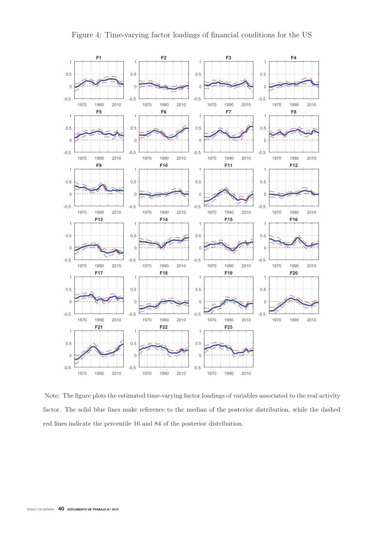
BANCO DE ESPAÑA 40 DOCUMENTO DE TRABAJO N.º 2018
Figure 4: Time-varying factor loadings of financial conditions for the US
1970 1990 2010-0.5
0
0.5
1F1
1970 1990 2010-0.5
0
0.5
1F2
1970 1990 2010-0.5
0
0.5
1F3
1970 1990 2010-0.5
0
0.5
1F4
1970 1990 2010-0.5
0
0.5
1F5
1970 1990 2010-0.5
0
0.5
1F6
1970 1990 2010-0.5
0
0.5
1F7
1970 1990 2010-0.5
0
0.5
1F8
1970 1990 2010-0.5
0
0.5
1F9
1970 1990 2010-0.5
0
0.5
1F10
1970 1990 2010-0.5
0
0.5
1F11
1970 1990 2010-0.5
0
0.5
1F12
1970 1990 2010-0.5
0
0.5
1F13
1970 1990 2010-0.5
0
0.5
1F14
1970 1990 2010-0.5
0
0.5
1F15
1970 1990 2010-0.5
0
0.5
1F16
1970 1990 2010-0.5
0
0.5
1F17
1970 1990 2010-0.5
0
0.5
1F18
1970 1990 2010-0.5
0
0.5
1F19
1970 1990 2010-0.5
0
0.5
1F20
1970 1990 2010-0.5
0
0.5
1F21
1970 1990 2010-0.5
0
0.5
1F22
1970 1990 2010-0.5
0
0.5
1F23
Note: The figure plots the estimated time-varying factor loadings of variables associated to the real activity
factor. The solid blue lines make reference to the median of the posterior distribution, while the dashed
red lines indicate the percentile 16 and 84 of the posterior distribution.

BANCO DE ESPAÑA 41 DOCUMENTO DE TRABAJO N.º 2018
Figure 5: Time-varying factor loadings of real activity for the US (cont.)
1970 1990 2010-0.5
0
0.5
1R1
1970 1990 2010-0.5
0
0.5
1R2
1970 1990 2010-0.5
0
0.5
1R3
1970 1990 2010-0.5
0
0.5
1R4
1970 1990 2010-0.5
0
0.5
1R5
1970 1990 2010-0.5
0
0.5
1R6
1970 1990 2010-0.5
0
0.5
1R7
1970 1990 2010-0.5
0
0.5
1R8
1970 1990 2010-0.5
0
0.5
1R9
Note: The figure plots the estimated time-varying factor loadings of variables associated to the financial
conditions factor. The solid blue lines make reference to the median of the posterior distribution, while
the dashed red lines indicate the percentile 16 and 84 of the posterior distribution.
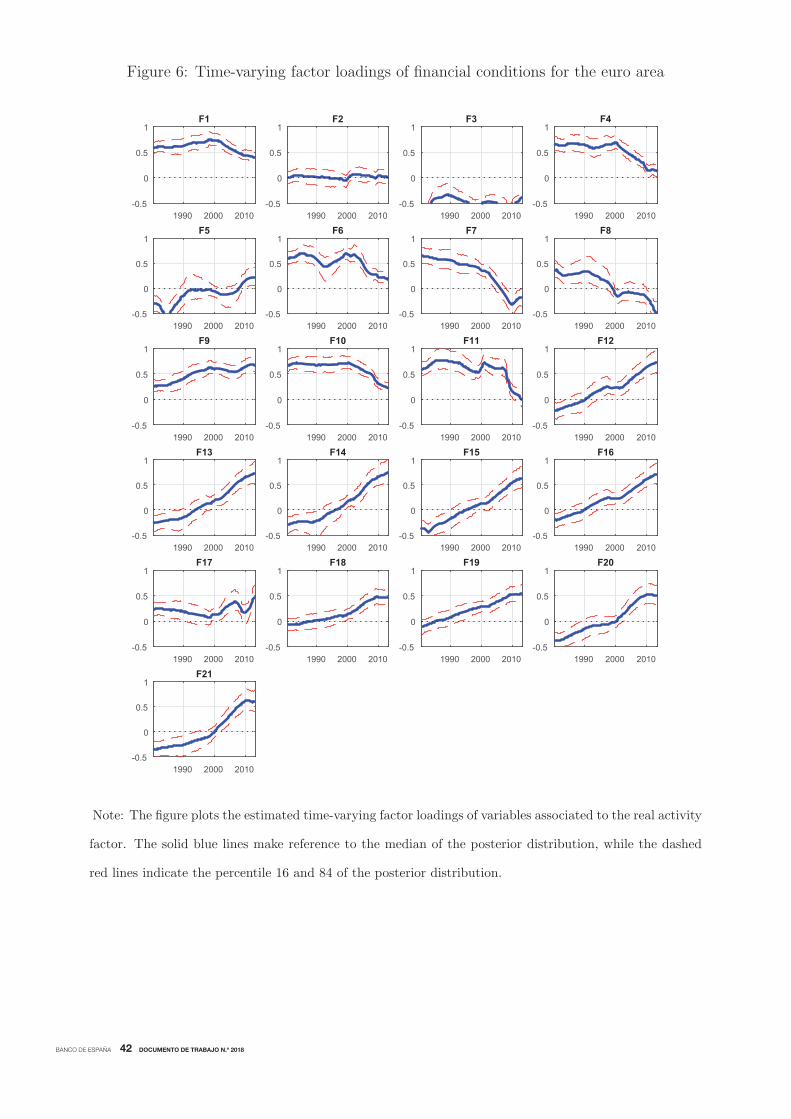
BANCO DE ESPAÑA 42 DOCUMENTO DE TRABAJO N.º 2018
Figure 6: Time-varying factor loadings of financial conditions for the euro area
1990 2000 2010-0.5
0
0.5
1F1
1990 2000 2010-0.5
0
0.5
1F2
1990 2000 2010-0.5
0
0.5
1F3
1990 2000 2010-0.5
0
0.5
1F4
1990 2000 2010-0.5
0
0.5
1F5
1990 2000 2010-0.5
0
0.5
1F6
1990 2000 2010-0.5
0
0.5
1F7
1990 2000 2010-0.5
0
0.5
1F8
1990 2000 2010-0.5
0
0.5
1F9
1990 2000 2010-0.5
0
0.5
1F10
1990 2000 2010-0.5
0
0.5
1F11
1990 2000 2010-0.5
0
0.5
1F12
1990 2000 2010-0.5
0
0.5
1F13
1990 2000 2010-0.5
0
0.5
1F14
1990 2000 2010-0.5
0
0.5
1F15
1990 2000 2010-0.5
0
0.5
1F16
1990 2000 2010-0.5
0
0.5
1F17
1990 2000 2010-0.5
0
0.5
1F18
1990 2000 2010-0.5
0
0.5
1F19
1990 2000 2010-0.5
0
0.5
1F20
1990 2000 2010-0.5
0
0.5
1F21
Note: The figure plots the estimated time-varying factor loadings of variables associated to the real activity
factor. The solid blue lines make reference to the median of the posterior distribution, while the dashed
red lines indicate the percentile 16 and 84 of the posterior distribution.
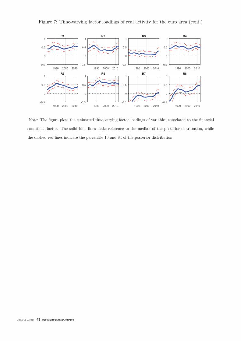
BANCO DE ESPAÑA 43 DOCUMENTO DE TRABAJO N.º 2018
Figure 7: Time-varying factor loadings of real activity for the euro area (cont.)
1990 2000 2010-0.5
0
0.5
1R1
1990 2000 2010-0.5
0
0.5
1R2
1990 2000 2010-0.5
0
0.5
1R3
1990 2000 2010-0.5
0
0.5
1R4
1990 2000 2010-0.5
0
0.5
1R5
1990 2000 2010-0.5
0
0.5
1R6
1990 2000 2010-0.5
0
0.5
1R7
1990 2000 2010-0.5
0
0.5
1R8
Note: The figure plots the estimated time-varying factor loadings of variables associated to the financial
conditions factor. The solid blue lines make reference to the median of the posterior distribution, while
the dashed red lines indicate the percentile 16 and 84 of the posterior distribution.

BANCO DE ESPAÑA 44 DOCUMENTO DE TRABAJO N.º 2018
Figure 8: Estimated correlation between factors of the US
1970 1980 1990 2000 20100.2
0.3
0.4
0.5
0.6
0.7
0.8
Figure 9: Estimated correlation between factors of the euro area
1985 1990 1995 2000 2005 20100.3
0.4
0.5
0.6
0.7
0.8
0.9
Note: The figures plot the estimated time-varying correlation between the real and financial cycle. The
solid blue line makes reference to the median of the posterior distribution, while the dashed red lines
indicate the percentile 16 and 84 of the posterior distribution.
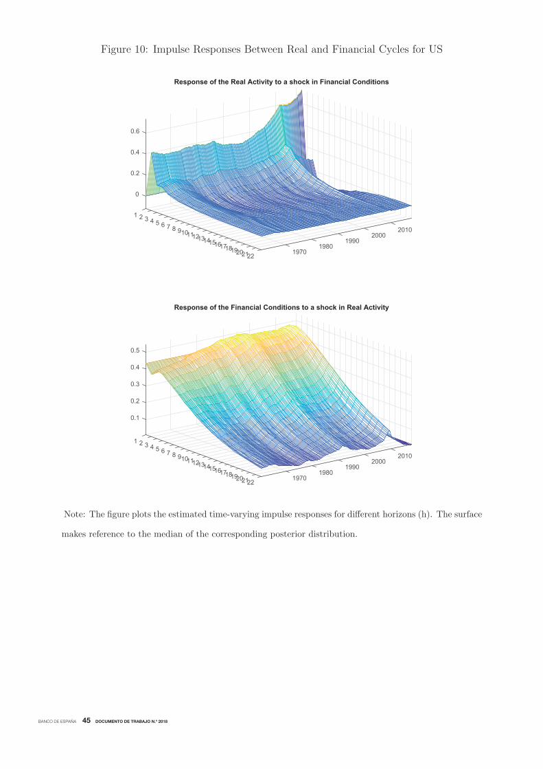
BANCO DE ESPAÑA 45 DOCUMENTO DE TRABAJO N.º 2018
Figure 10: Impulse Responses Between Real and Financial Cycles for US
1
0
2 3 4
0.2
5 6 7 8
0.4
2010910
Response of the Real Activity to a shock in Financial Conditions
11 200012
0.6
1314 1990151617 19801819 1970202122
1
0.1
2 3 4
0.2
5 6 7
0.3
8 2010910
0.4
Response of the Financial Conditions to a shock in Real Activity
11 20001213
0.5
14 1990151617 19801819 1970202122
Note: The figure plots the estimated time-varying impulse responses for different horizons (h). The surface
makes reference to the median of the corresponding posterior distribution.
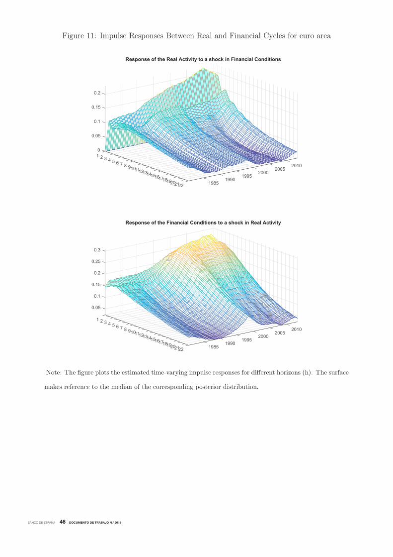
BANCO DE ESPAÑA 46 DOCUMENTO DE TRABAJO N.º 2018
Figure 11: Impulse Responses Between Real and Financial Cycles for euro area
01 2
0.05
3 4 5
0.1
6 7 20108 9
0.15
10
Response of the Real Activity to a shock in Financial Conditions
20051112
0.2
2000131415 19951617 1990181920 19852122
0.05
1 2 3
0.1
4 5
0.15
6 7 20108
0.2
910
Response of the Financial Conditions to a shock in Real Activity
200511
0.25
12 20001314
0.3
15 19951617 1990181920 19852122
Note: The figure plots the estimated time-varying impulse responses for different horizons (h). The surface
makes reference to the median of the corresponding posterior distribution.

BANCO DE ESPAÑA 47 DOCUMENTO DE TRABAJO N.º 2018
Figure 12: Estimated correlation between real and financial factors of US and E.A. (Two-economy model)
1985 1990 1995 2000 2005 2010-0.4
-0.2
0
0.2
0.4
0.6
Financial U.S. and Financial E.A.
1985 1990 1995 2000 2005 2010
0
0.1
0.2
0.3
0.4
0.5
0.6
0.7
Financial U.S. and Real E.A.
1985 1990 1995 2000 2005 2010
-0.1
0
0.1
0.2
0.3
0.4
0.5Real U.S. and Financial E.A.
1985 1990 1995 2000 2005 2010-0.2
-0.1
0
0.1
0.2
0.3
0.4
0.5
Real U.S. and Real E.A.
Note: The figures plot the estimated time-varying correlation between the real and financial cycle associated to the US and euro area. The solid blueline makes reference to the median of the posterior distribution, while the dashed red lines indicate the percentile 16 and 84 of the posterior distribution.

BANCO DE ESPAÑA 48 DOCUMENTO DE TRABAJO N.º 2018
Figure 13: Macro-financial spillovers from the US to the euro area over time (Two-economy model)
01 2
0.1
3 4 5 6
0.2
7 8 20109
0.3
10
Response of the E.A. Real Activity to a shock in U.S. Real Activity
20051112
0.4
2000131415 19951617 1990181920 19852122
-0.11 2 3 4
0
5 6 7 8 20109
0.1
10
Response of the E.A. Real Activity to a shock in U.S. Financial Conditions
20051112 2000131415 19951617 1990181920 19852122
1
0.05
2 3 4 5
0.1
6 7 8 2010
0.15
910
Response of the E.A. Financial Conditions to a shock in U.S. Real Activity
200511
0.2
12 2000131415 19951617 1990181920 19852122
1 2 3
0.05
4 5 6 7 8 2010
0.1
910
Response of the E.A. Financial Conditions to a shock in U.S. Financial Conditions
20051112 200013
0.15
1415 19951617 1990181920 19852122
Note: The figure plots the estimated time-varying impulse responses for different horizons (h). The surface makes reference to the median of thecorresponding posterior distribution. The estimates are obtained by using sign and exclusion restrictions in the impact multiplier matrix to identifythe structural shocks.

BANCO DE ESPAÑA 49 DOCUMENTO DE TRABAJO N.º 2018
Figure 14: Macro-financial spillovers from the euro area to the US over time (Two-economy model)
-0.05
1 2 3
0
4 5 6
0.05
7 8 20109
0.1
10
Response of the U.S. Real Activity to a shock in E.A. Real Activity
20051112
0.15
2000131415 19951617 1990181920 19852122
-0.051 2 3
0
4 5 6 7
0.05
8 2010910
Response of the U.S. Real Activity to a shock in E.A. Financial Conditions
200511
0.1
12 2000131415 19951617 1990181920 19852122
1
-0.06
2 3 4 5
-0.04
6 7 8 2010
-0.02
910
Response of the U.S. Financial Conditions to a shock in E.A. Real Activity
20051112
0
2000131415 19951617 1990181920 19852122
-0.081 2 3
-0.06
4 5 6 7
-0.04
8 2010910
Response of the U.S. Financial Conditions to a shock in E.A. Financial Conditions
2005
-0.02
1112 2000131415 19951617 1990181920 19852122
Note: The figure plots the estimated time-varying impulse responses for different horizons (h). The surface makes reference to the median of thecorresponding posterior distribution. The estimates are obtained by using sign and exclusion restrictions in the impact multiplier matrix to identifythe structural shocks.
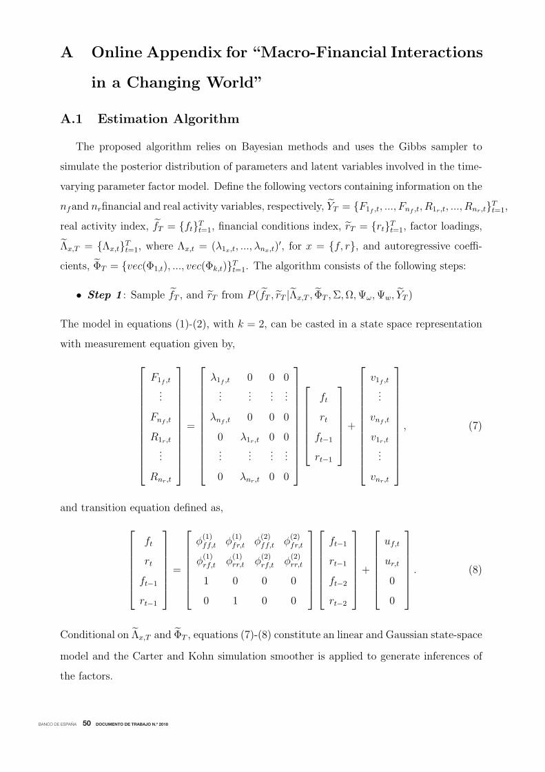
BANCO DE ESPAÑA 50 DOCUMENTO DE TRABAJO N.º 2018
A Online Appendix for “Macro-Financial Interactions
in a Changing World”
A.1 Estimation Algorithm
The proposed algorithm relies on Bayesian methods and uses the Gibbs sampler to
simulate the posterior distribution of parameters and latent variables involved in the time-
varying parameter factor model. Define the following vectors containing information on the
nfand nrfinancial and real activity variables, respectively, YT = {F1f ,t, ..., Fnf ,t, R1r,t, ..., Rnr,t}Tt=1,
real activity index, fT = {ft}Tt=1, financial conditions index, rT = {rt}Tt=1, factor loadings,
Λx,T = {Λx,t}Tt=1, where Λx,t = (λ1x,t, ..., λnx,t)′, for x = {f, r}, and autoregressive coeffi-
cients, ΦT = {vec(Φ1,t), ..., vec(Φk,t)}Tt=1. The algorithm consists of the following steps:
• Step 1 : Sample fT , and rT from P (fT , rT |Λx,T , ΦT ,Σ,Ω,Ψω,Ψw, YT )
The model in equations (1)-(2), with k = 2, can be casted in a state space representation
with measurement equation given by,
⎡⎢⎢⎢⎢⎢⎢⎢⎢⎢⎢⎢⎢⎣
F1f ,t
...
Fnf ,t
R1r,t
...
Rnr,t
⎤⎥⎥⎥⎥⎥⎥⎥⎥⎥⎥⎥⎥⎦
=
⎡⎢⎢⎢⎢⎢⎢⎢⎢⎢⎢⎢⎢⎣
λ1f ,t 0 0 0...
......
...
λnf ,t 0 0 0
0 λ1r,t 0 0...
......
...
0 λnr,t 0 0
⎤⎥⎥⎥⎥⎥⎥⎥⎥⎥⎥⎥⎥⎦
⎡⎢⎢⎢⎢⎢⎢⎣
ft
rt
ft−1
rt−1
⎤⎥⎥⎥⎥⎥⎥⎦+
⎡⎢⎢⎢⎢⎢⎢⎢⎢⎢⎢⎢⎢⎣
v1f ,t...
vnf ,t
v1r,t...
vnr,t
⎤⎥⎥⎥⎥⎥⎥⎥⎥⎥⎥⎥⎥⎦
, (7)
and transition equation defined as,
⎡⎢⎢⎢⎢⎢⎢⎣
ft
rt
ft−1
rt−1
⎤⎥⎥⎥⎥⎥⎥⎦=
⎡⎢⎢⎢⎢⎢⎢⎣
φ(1)ff,t φ
(1)fr,t φ
(2)ff,t φ
(2)fr,t
φ(1)rf,t φ
(1)rr,t φ
(2)rf,t φ
(2)rr,t
1 0 0 0
0 1 0 0
⎤⎥⎥⎥⎥⎥⎥⎦
⎡⎢⎢⎢⎢⎢⎢⎣
ft−1
rt−1
ft−2
rt−2
⎤⎥⎥⎥⎥⎥⎥⎦+
⎡⎢⎢⎢⎢⎢⎢⎣
uf,t
ur,t
0
0
⎤⎥⎥⎥⎥⎥⎥⎦. (8)
Conditional on Λx,T and ΦT , equations (7)-(8) constitute an linear and Gaussian state-space
model and the Carter and Kohn simulation smoother is applied to generate inferences of
the factors.
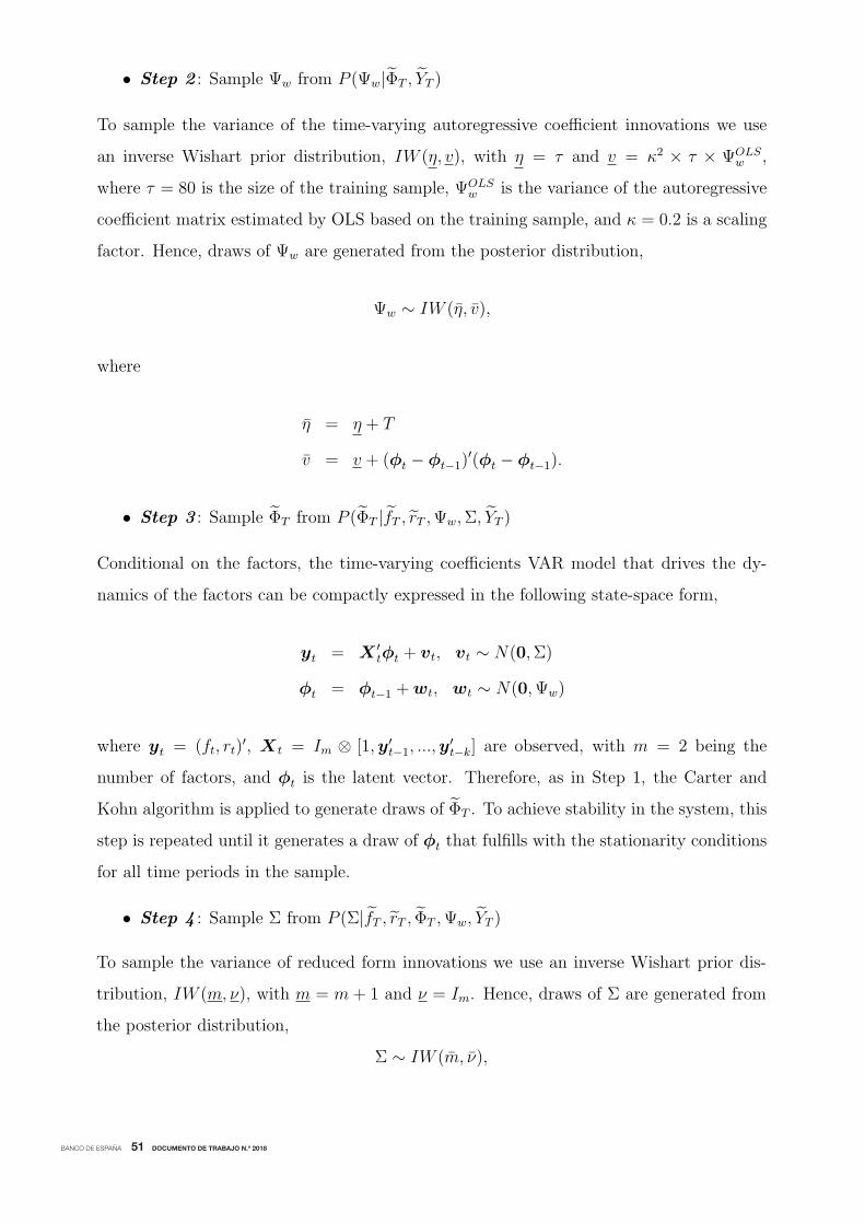
BANCO DE ESPAÑA 51 DOCUMENTO DE TRABAJO N.º 2018
• Step 2 : Sample Ψw from P (Ψw|ΦT , YT )
To sample the variance of the time-varying autoregressive coefficient innovations we use
an inverse Wishart prior distribution, IW (η, v), with η = τ and v = κ2 × τ × ΨOLSw ,
where τ = 80 is the size of the training sample, ΨOLSw is the variance of the autoregressive
coefficient matrix estimated by OLS based on the training sample, and κ = 0.2 is a scaling
factor. Hence, draws of Ψw are generated from the posterior distribution,
Ψw ∼ IW (η, v),
where
η = η + T
v = v + (φt − φt−1)′(φt − φt−1).
• Step 3 : Sample ΦT from P (ΦT |fT , rT ,Ψw,Σ, YT )
Conditional on the factors, the time-varying coefficients VAR model that drives the dy-
namics of the factors can be compactly expressed in the following state-space form,
yt = X ′tφt + vt, vt ∼ N(0,Σ)
φt = φt−1 +wt, wt ∼ N(0,Ψw)
where yt = (ft, rt)′, X t = Im ⊗ [1,y′t−1, ...,y
′t−k] are observed, with m = 2 being the
number of factors, and φt is the latent vector. Therefore, as in Step 1, the Carter and
Kohn algorithm is applied to generate draws of ΦT . To achieve stability in the system, this
step is repeated until it generates a draw of φt that fulfills with the stationarity conditions
for all time periods in the sample.
• Step 4 : Sample Σ from P (Σ|fT , rT , ΦT ,Ψw, YT )
To sample the variance of reduced form innovations we use an inverse Wishart prior dis-
tribution, IW (m, ν), with m = m + 1 and ν = Im. Hence, draws of Σ are generated from
the posterior distribution,
Σ ∼ IW (m, ν),

BANCO DE ESPAÑA 52 DOCUMENTO DE TRABAJO N.º 2018
where
m = m+ T
ν = ν + (yt −X ′tφt)
′(yt −X ′tφt).
• Step 5 : Sample Λx,T from P (Λx,T |fT , rT ,Ω,Ψω, YT )
Given that Ω is assumed to be a diagonal matrix, each time-varying loading can be sampled
independently. Accordingly, we use the following state-space representation,
Xix,t = λix,txt + vix,t, vix,t ∼ N(0,Ω[ix,ix])
λix,t = λix,t−1 + ωix,t, ωix,t ∼ N(0,Ψω,[ix,ix])
for observed variables X = F,R, latent factors x = f, r, and i = 1, ..., n. Next, the Carter
and Kohn algorithm is applied to generate draws of the elements in Λx,T .
• Step 6 : Sample Ψω from P (Ψω|Λx,T , YT )
To sample, independently, the variance of the time-varying loading innovations we use an
inverse Gamma prior distribution, IG(u, z), with u = 0.1× T and z = 0.12. Hence, draws
of Ψw are generated from the posterior distribution,
Ψw ∼ IG(u, z),
where
u = u+ T
z = z + (λix,t − λix,t−1)′(λix,t − λix,t−1).
• Step 7 : Sample Ω from P (Ω|fT , rT , Λx,T , YT )
To sample, independently, the variance of the idiosyncratic terms we use an inverse Gamma
prior distribution, IG(l, o), with l = 0 and o = 0. Accordingly, draws of the entries in the
diagonal of Ω are generated from the posterior distribution,
Ωix ∼ IG(l, o),

BANCO DE ESPAÑA 53 DOCUMENTO DE TRABAJO N.º 2018
for i = 1, ..., n, X = F,R, and x = f, r, where
l = l + T
o = o+ (Xix,t − λix,txt)′(Xix,t − λix,txt).
To approximate the posterior distribution of both the parameters and latent variables
involved in the model, each step of the algorithm is recursively repeated M = 22, 000 times,
discarding the first m = 20, 000 iterations to ensure convergence.
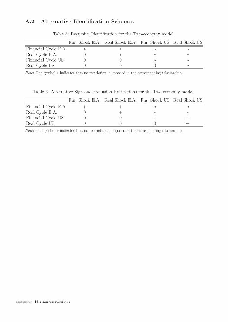
BANCO DE ESPAÑA 54 DOCUMENTO DE TRABAJO N.º 2018
A.2 Alternative Identification Schemes
Table 5: Recursive Identification for the Two-economy model
Fin. Shock E.A. Real Shock E.A. Fin. Shock US Real Shock US
Financial Cycle E.A. ∗ ∗ ∗ ∗Real Cycle E.A. 0 ∗ ∗ ∗Financial Cycle US 0 0 ∗ ∗Real Cycle US 0 0 0 ∗Note: The symbol ∗ indicates that no restriction is imposed in the corresponding relationship.
Table 6: Alternative Sign and Exclusion Restrictions for the Two-economy model
Fin. Shock E.A. Real Shock E.A. Fin. Shock US Real Shock US
Financial Cycle E.A. + + ∗ ∗Real Cycle E.A. 0 + ∗ ∗Financial Cycle US 0 0 + +Real Cycle US 0 0 0 +
Note: The symbol ∗ indicates that no restriction is imposed in the corresponding relationship.

BANCO DE ESPAÑA 55 DOCUMENTO DE TRABAJO N.º 2018
A.3 Additional Figures
Figure 15: Estimated factors of the US - Principal Component
1965 1970 1975 1980 1985 1990 1995 2000 2005 2010 2015
-5
0
5
-1.5
-1
-0.5
0
0.5
1(a) Financial Cycle
1965 1970 1975 1980 1985 1990 1995 2000 2005 2010 2015
-10
-5
0
5
-2
-1
0
1
(b) Real Cycle
Figure 16: Estimated factors of the euro area - Principal Component
1985 1990 1995 2000 2005 2010
-2
0
2
4
-1
-0.5
0
0.5
1
1.5(a) Financial Cycle
1985 1990 1995 2000 2005 2010-6
-4
-2
0
2
4
-1.5
-1
-0.5
0
0.5
1
(b) Real Cycle
Note: The figures plot the estimated real and financial cycles. The solid blue lines make reference to
the median of the posterior distribution, while the dashed red lines indicate the percentile 5 and 95 of
the posterior distribution, and the solid green line plots the corresponding factor estimated with principal
components, and aligned with the right axis.
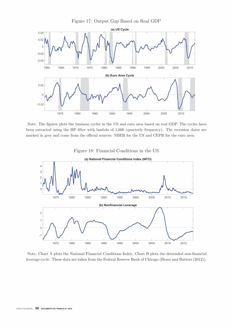
BANCO DE ESPAÑA 56 DOCUMENTO DE TRABAJO N.º 2018
Figure 17: Output Gap Based on Real GDP
1960 1965 1970 1975 1980 1985 1990 1995 2000 2005 2010
-0.04
-0.02
0
0.02
0.04(a) US Cycle
1975 1980 1985 1990 1995 2000 2005 2010
-0.02
0
0.02
(b) Euro Area Cycle
Note: The figures plots the business cycles in the US and euro area based on real GDP. The cycles have
been extracted using the HP filter with lambda of 1,600 (quarterly frequency). The recession dates are
marked in grey and come from the official sources: NBER for the US and CEPR for the euro area.
Figure 18: Financial Conditions in the US
1975 1980 1985 1990 1995 2000 2005 2010 2015
0
1
2
3
4
(a) National Financial Conditions Index (NFCI)
1975 1980 1985 1990 1995 2000 2005 2010 2015
-1
0
1
2
(b) Nonfinancial Leverage
Note: Chart A plots the National Financial Conditions Index. Chart B plots the detrended non-financial
leverage cycle. These data are taken from the Federal Reserve Bank of Chicago (Brave and Butters (2012)).

BANCO DE ESPAÑA 57 DOCUMENTO DE TRABAJO N.º 2018
Figure 19: Estimated correlation between factors of the US - Orthogonal Innovations
1970 1980 1990 2000 2010-0.2
0
0.2
0.4
0.6
0.8
1
Figure 20: Estimated correlation between factors of the euro area - Orthogonal Innovations
1985 1990 1995 2000 2005 2010-0.1
0
0.1
0.2
0.3
0.4
0.5
0.6
0.7
0.8
0.9
Note: The figures plot the estimated time-varying correlation between the real and financial cycle. The
solid blue line makes reference to the median of the posterior distribution, while the dashed red lines
indicate the percentile 16 and 84 of the posterior distribution. The estimates are obtained by assuming
orthogonality in the innovations of the factors.

BANCO DE ESPAÑA 58 DOCUMENTO DE TRABAJO N.º 2018
Figure 21: Estimated correlation between factors of the US - Break in Volatility
1970 1980 1990 2000 20100.2
0.3
0.4
0.5
0.6
0.7
0.8
Note: The figure plots the estimated time-varying correlation between the real and financial cycles. The
solid blue line makes reference to the median of the posterior distribution, while the dashed red lines
indicate the percentile 16 and 84 of the posterior distribution. The estimates are obtained by assuming a
break in the volatility of the factors occurred in 1985.
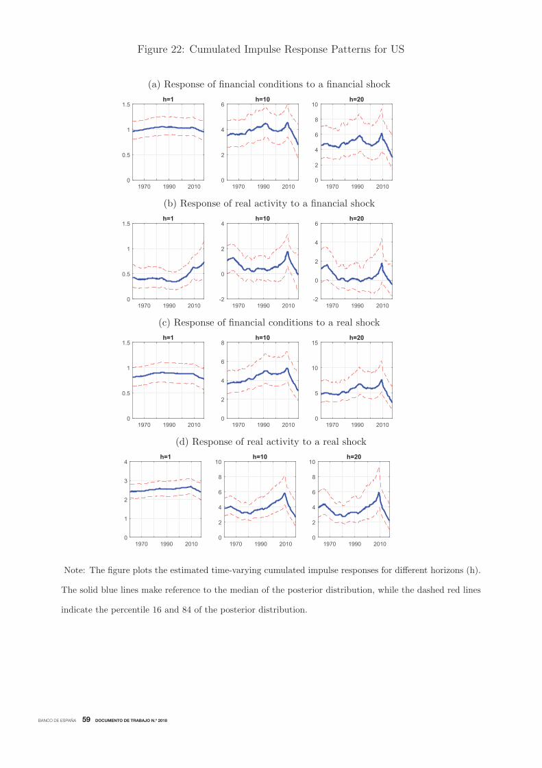
BANCO DE ESPAÑA 59 DOCUMENTO DE TRABAJO N.º 2018
Figure 22: Cumulated Impulse Response Patterns for US
(a) Response of financial conditions to a financial shock
1970 1990 20100
0.5
1
1.5h=1
1970 1990 20100
2
4
6h=10
1970 1990 20100
2
4
6
8
10h=20
(b) Response of real activity to a financial shock
1970 1990 20100
0.5
1
1.5h=1
1970 1990 2010-2
0
2
4h=10
1970 1990 2010-2
0
2
4
6h=20
(c) Response of financial conditions to a real shock
1970 1990 20100
0.5
1
1.5h=1
1970 1990 20100
2
4
6
8h=10
1970 1990 20100
5
10
15h=20
(d) Response of real activity to a real shock
1970 1990 20100
1
2
3
4h=1
1970 1990 20100
2
4
6
8
10h=10
1970 1990 20100
2
4
6
8
10h=20
Note: The figure plots the estimated time-varying cumulated impulse responses for different horizons (h).
The solid blue lines make reference to the median of the posterior distribution, while the dashed red lines
indicate the percentile 16 and 84 of the posterior distribution.

BANCO DE ESPAÑA 60 DOCUMENTO DE TRABAJO N.º 2018
Figure 23: Cumulated Impulse Response Patterns for euro area
(a) Response of financial conditions to a financial shock
1990 2000 20100
0.2
0.4
0.6
0.8h=1
1990 2000 20100
1
2
3
4h=10
1990 2000 20100
2
4
6h=20
(b) Response of real activity to a financial shock
1990 2000 20100
0.1
0.2
0.3
0.4h=1
1990 2000 2010-0.5
0
0.5
1
1.5
2h=10
1990 2000 2010-1
0
1
2
3
4h=20
(c) Response of financial conditions to a real shock
1990 2000 20100
0.2
0.4
0.6h=1
1990 2000 20100
1
2
3
4h=10
1990 2000 20100
2
4
6
8h=20
(d) Response of real activity to a real shock
1990 2000 20100
0.5
1
1.5
2h=1
1990 2000 20100
2
4
6h=10
1990 2000 20100
2
4
6
8h=20
Note: The figure plots the estimated time-varying cumulated impulse responses for different horizons (h).
The solid blue lines make reference to the median of the posterior distribution, while the dashed red lines
indicate the percentile 16 and 84 of the posterior distribution.
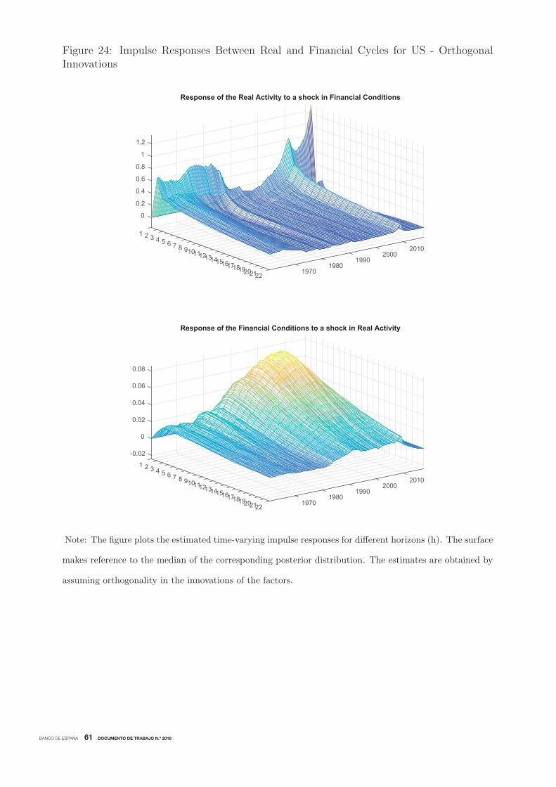
BANCO DE ESPAÑA 61 DOCUMENTO DE TRABAJO N.º 2018
Figure 24: Impulse Responses Between Real and Financial Cycles for US - OrthogonalInnovations
0
1 2
0.2
3 4
0.4
5 6
0.6
7 8 2010
0.8
910
Response of the Real Activity to a shock in Financial Conditions
1
11 200012
1.2
1314 1990151617 19801819 1970202122
-0.02
1 2
0
3 4 5
0.02
6 7 8
0.04
2010910
Response of the Financial Conditions to a shock in Real Activity
0.06
11 20001213
0.08
14 1990151617 19801819 1970202122
Note: The figure plots the estimated time-varying impulse responses for different horizons (h). The surface
makes reference to the median of the corresponding posterior distribution. The estimates are obtained by
assuming orthogonality in the innovations of the factors.

BANCO DE ESPAÑA 62 DOCUMENTO DE TRABAJO N.º 2018
Figure 25: Impulse Responses Between Real and Financial Cycles for euro area - OrthogonalInnovations
01 2 3
0.1
4 5 6 7
0.2
20108 910
Response of the Real Activity to a shock in Financial Conditions
200511
0.3
12 2000131415 19951617 1990181920 19852122
01 2 3
0.05
4 5 6 7
0.1
20108 910
Response of the Financial Conditions to a shock in Real Activity
200511
0.15
12 2000131415 19951617 1990181920 19852122
Note: The figure plots the estimated time-varying impulse responses for different horizons (h). The surface
makes reference to the median of the corresponding posterior distribution. The estimates are obtained by
assuming orthogonality in the innovations of the factors.
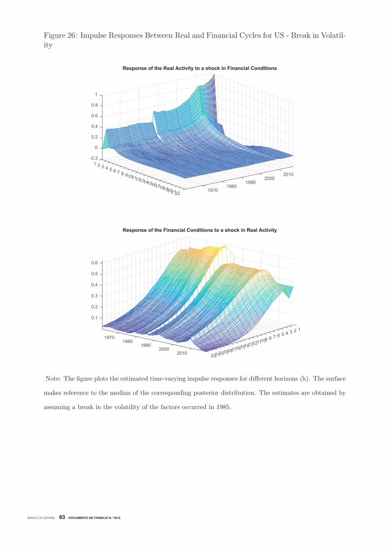
BANCO DE ESPAÑA 63 DOCUMENTO DE TRABAJO N.º 2018
Figure 26: Impulse Responses Between Real and Financial Cycles for US - Break in Volatil-ity
-0.21
0
2 3 4
0.2
5 6
0.4
7 8 20109
0.6
10
Response of the Real Activity to a shock in Financial Conditions
11 2000
0.8
121314
1
1990151617 19801819 1970202122
1234
0.1
567
0.2
1970 8
Response of the Financial Conditions to a shock in Real Activity
9
0.3
101980 11
0.4
12131990
0.5
141516
0.6
2000 1718192010 202122
Note: The figure plots the estimated time-varying impulse responses for different horizons (h). The surface
makes reference to the median of the corresponding posterior distribution. The estimates are obtained by
assuming a break in the volatility of the factors occurred in 1985.

BANCO DE ESPAÑA 64 DOCUMENTO DE TRABAJO N.º 2018
Figure 27: Forecast Error Variance Decomposition for US
(a) Contribution of financial shocks to financial conditions
1970 1990 20100
0.2
0.4
0.6
0.8
1h=1
1970 1990 20100
0.2
0.4
0.6
0.8
1h=10
1970 1990 20100
0.2
0.4
0.6
0.8
1h=20
(b) Contribution of financial shocks to real activity
1970 1990 20100
0.2
0.4
0.6
0.8
1h=1
1970 1990 20100
0.2
0.4
0.6
0.8
1h=10
1970 1990 20100
0.2
0.4
0.6
0.8
1h=20
(c) Contribution of real shocks to financial conditions
1970 1990 20100
0.2
0.4
0.6
0.8
1h=1
1970 1990 20100
0.2
0.4
0.6
0.8
1h=10
1970 1990 20100
0.2
0.4
0.6
0.8
1h=20
(d) Contribution of real shocks to real activity
1970 1990 20100
0.2
0.4
0.6
0.8
1h=1
1970 1990 20100
0.2
0.4
0.6
0.8
1h=10
1970 1990 20100
0.2
0.4
0.6
0.8
1h=20
Note: The figure plots the estimated time-varying forecast error variance decomposition for different
horizons (h). The solid blue lines make reference to the median of the posterior distribution, while the
dashed red lines indicate the percentile 16 and 84 of the posterior distribution.

BANCO DE ESPAÑA 65 DOCUMENTO DE TRABAJO N.º 2018
Figure 28: Forecast Error Variance Decomposition for euro area
(a) Contribution of financial shocks to financial conditions
1990 2000 20100
0.2
0.4
0.6
0.8
1h=1
1990 2000 20100
0.2
0.4
0.6
0.8
1h=10
1990 2000 20100
0.2
0.4
0.6
0.8
1h=20
(b) Contribution of financial shocks to real activity
1990 2000 20100
0.2
0.4
0.6
0.8
1h=1
1990 2000 20100
0.2
0.4
0.6
0.8
1h=10
1990 2000 20100
0.2
0.4
0.6
0.8
1h=20
(c) Contribution of real shocks to financial conditions
1990 2000 20100
0.2
0.4
0.6
0.8
1h=1
1990 2000 20100
0.2
0.4
0.6
0.8
1h=10
1990 2000 20100
0.2
0.4
0.6
0.8
1h=20
(d) Contribution real shocks to real activity
1990 2000 20100
0.2
0.4
0.6
0.8
1h=1
1990 2000 20100
0.2
0.4
0.6
0.8
1h=10
1990 2000 20100
0.2
0.4
0.6
0.8
1h=20
Note: The figure plots the estimated time-varying forecast error variance decomposition for different
horizons (h). The solid blue lines make reference to the median of the posterior distribution, while the
dashed red lines indicate the percentile 16 and 84 of the posterior distribution.
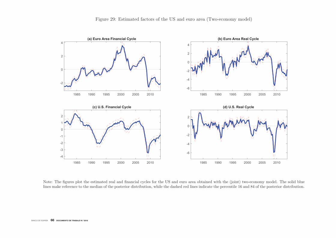
BANCO DE ESPAÑA 66 DOCUMENTO DE TRABAJO N.º 2018
Figure 29: Estimated factors of the US and euro area (Two-economy model)
1985 1990 1995 2000 2005 2010
-2
0
2
4(a) Euro Area Financial Cycle
1985 1990 1995 2000 2005 2010
-6
-4
-2
0
2
4
(b) Euro Area Real Cycle
1985 1990 1995 2000 2005 2010
-4
-3
-2
-1
0
1
2
(c) U.S. Financial Cycle
1985 1990 1995 2000 2005 2010
-6
-4
-2
0
2
(d) U.S. Real Cycle
Note: The figures plot the estimated real and financial cycles for the US and euro area obtained with the (joint) two-economy model. The solid bluelines make reference to the median of the posterior distribution, while the dashed red lines indicate the percentile 16 and 84 of the posterior distribution.

BANCO DE ESPAÑA 67 DOCUMENTO DE TRABAJO N.º 2018
Figure 30: Estimated correlation between factors associated to a given economy (Two-economy model)
1985 1990 1995 2000 2005 2010
0.1
0.2
0.3
0.4
0.5
0.6
0.7(a) Real and Financial of U.S.
1985 1990 1995 2000 2005 2010
0.2
0.3
0.4
0.5
0.6
0.7
0.8
(b) Real and Financial of E.A.
Note: The figure plots the estimated time-varying correlation between the business and financial cycles as-
sociated to a given economy. The solid blue line makes reference to the median of the posterior distribution,
while the dashed red lines indicate the percentile 16 and 84 of the posterior distribution.

BANCO DE ESPAÑA 68 DOCUMENTO DE TRABAJO N.º 2018
Figure 31: Cumulated Impulse Response Patterns: Effect of US on E.A.
(a) Response of the E.A. Real Activity to a shock in US Real Activity
1990 2000 20100
0.5
1
1.5h=1
1990 2000 20100
1
2
3
4
5h=10
1990 2000 20100
2
4
6h=20
(b) Response of the E.A. Real Activity to a shock in US FinancialConditions
1990 2000 2010-0.4
-0.2
0
0.2
0.4h=1
1990 2000 2010-1
0
1
2
3h=10
1990 2000 2010-2
0
2
4
6h=20
(c) Response of the E.A. Financial Conditions to a shock in US RealActivity
1990 2000 20100
0.2
0.4
0.6h=1
1990 2000 20100
1
2
3
4h=10
1990 2000 2010-2
0
2
4
6
8h=20
(d) Response of the E.A. Financial Conditions to a shock in USFinancial Conditions
1990 2000 2010-0.4
-0.2
0
0.2
0.4h=1
1990 2000 2010-2
-1
0
1
2
3h=10
1990 2000 2010-2
0
2
4
6h=20
Note: The figure plots the estimated time-varying cumulated impulse responses for different horizons (h).
The solid blue lines make reference to the median of the posterior distribution, while the dashed red lines
indicate the percentile 16 and 84 of the posterior distribution.

BANCO DE ESPAÑA 69 DOCUMENTO DE TRABAJO N.º 2018
Figure 32: Cumulated Impulse Response Patterns: Effect of E.A. on US
(a) Response of the US Real Activity to a shock in E.A. Real Activity
1990 2000 2010-0.1
0
0.1
0.2
0.3
0.4h=1
1990 2000 2010-2
-1
0
1
2h=10
1990 2000 2010-2
-1
0
1
2h=20
(b) Response of the US Real Activity to a shock in E.A. FinancialConditions
1990 2000 2010-0.2
0
0.2
0.4
0.6h=1
1990 2000 2010-2
-1
0
1
2h=10
1990 2000 2010-2
-1
0
1
2h=20
(c) Response of the US Financial Conditions to a shock in E.A. RealActivity
1990 2000 2010-0.1
-0.05
0
0.05
0.1h=1
1990 2000 2010-1.5
-1
-0.5
0
0.5
1h=10
1990 2000 2010-3
-2
-1
0
1h=20
(d) Response of the US Financial Conditions to a shock in E.A.Financial Conditions
1990 2000 2010-1
-0.5
0
0.5
1h=1
1990 2000 2010-3
-2
-1
0
1
2h=10
1990 2000 2010-4
-2
0
2h=20
Note: The figure plots the estimated time-varying cumulated impulse responses for different horizons (h).
The solid blue lines make reference to the median of the posterior distribution, while the dashed red lines
indicate the percentile 16 and 84 of the posterior distribution.

BANCO DE ESPAÑA 70 DOCUMENTO DE TRABAJO N.º 2018
Figure 33: Macro-financial spillovers from the US to the euro area over time - Cholesky
-0.11 2 3
0
4 5 6 7
0.1
8 2010910
Response of the E.A. Real Activity to a shock in U.S. Real Activity
200511
0.2
12 2000131415 19951617 1990181920 19852122
0
1 2 3 4
0.1
5 6 7 8 20109
0.2
10
Response of the E.A. Real Activity to a shock in U.S. Financial Conditions
20051112 2000131415 19951617 1990181920 19852122
1
0.05
2 3 4 5
0.1
6 7 8 2010
0.15
910
Response of the E.A. Financial Conditions to a shock in U.S. Real Activity
20051112
0.2
2000131415 19951617 1990181920 19852122
1 2
0.05
3 4 5 6
0.1
7 8 2010910
0.15
Response of the E.A. Financial Conditions to a shock in U.S. Financial Conditions
20051112 200013
0.2
1415 19951617 1990181920 19852122
Note: The figure plots the estimated time-varying impulse responses for different horizons (h). The surface makes reference to the median of thecorresponding posterior distribution. The estimates are obtained by using Cholesky factorization to identify the structural shocks.

BANCO DE ESPAÑA 71 DOCUMENTO DE TRABAJO N.º 2018
Figure 34: Macro-financial spillovers from the euro area to the US over time - Cholesky
1 2
0
3 4 5 6
0.1
7 8 2010910
Response of the U.S. Real Activity to a shock in E.A. Real Activity
200511
0.2
12 2000131415 19951617 1990181920 19852122
1 2
-0.05
3 4 5 6
0
7 8 2010910
Response of the U.S. Real Activity to a shock in E.A. Financial Conditions
0.05
20051112 2000131415 19951617 1990181920 19852122
-0.11 2 3 4
-0.05
5 6 7 8 20109
0
10
Response of the U.S. Financial Conditions to a shock in E.A. Real Activity
20051112 2000131415 19951617 1990181920 19852122
1 2
-0.06
3 4 5 6
-0.04
7 8 2010910
-0.02
Response of the U.S. Financial Conditions to a shock in E.A. Financial Conditions
20051112 20001314
0
15 19951617 1990181920 19852122
Note: The figure plots the estimated time-varying impulse responses for different horizons (h). The surface makes reference to the median of thecorresponding posterior distribution. The estimates are obtained by using Cholesky factorization to identify the structural shocks.

BANCO DE ESPAÑA 72 DOCUMENTO DE TRABAJO N.º 2018
Figure 35: Macro-financial spillovers from the US to the euro area over time - Alternative sign and exclusion restrictions
-0.1
1 2 3
0
4 5 6 7 8
0.1
2010910
Response of the E.A. Real Activity to a shock in U.S. Real Activity
20051112
0.2
2000131415 19951617 1990181920 19852122
0
1 2 3 4
0.1
5 6 7 8 20109
0.2
10
Response of the E.A. Real Activity to a shock in U.S. Financial Conditions
20051112 20001314
0.3
15 19951617 1990181920 19852122
1 2
0.05
3 4 5
0.1
6 7 8 20109
0.15
10
Response of the E.A. Financial Conditions to a shock in U.S. Real Activity
20051112
0.2
2000131415 19951617 1990181920 19852122
1 2
0.05
3 4 5 6
0.1
7 8 20109
0.15
10
Response of the E.A. Financial Conditions to a shock in U.S. Financial Conditions
20051112 200013
0.2
1415 19951617 1990181920 19852122
Note: The figure plots the estimated time-varying impulse responses for different horizons (h). The surface makes reference to the median of thecorresponding posterior distribution. The estimates are obtained by using Cholesky factorization to identify the structural shocks.

BANCO DE ESPAÑA 73 DOCUMENTO DE TRABAJO N.º 2018
Figure 36: Macro-financial spillovers from the euro area to the US over time - Alternative sign and exclusion restrictions
1 2
0
3 4 5 6
0.1
7 8 2010910
Response of the U.S. Real Activity to a shock in E.A. Real Activity
200511
0.2
12 2000131415 19951617 1990181920 19852122
1
-0.05
2 3 4 5 6
0
7 8 2010910
0.05
Response of the U.S. Real Activity to a shock in E.A. Financial Conditions
20051112 20001314
0.1
15 19951617 1990181920 19852122
-0.11 2 3 4
-0.05
5 6 7 8 20109
0
10
Response of the U.S. Financial Conditions to a shock in E.A. Real Activity
20051112 20001314
0.05
15 19951617 1990181920 19852122
-0.081 2 3
-0.06
4 5 6
-0.04
7 8 2010910
Response of the U.S. Financial Conditions to a shock in E.A. Financial Conditions
2005
-0.02
1112 20001314
0
15 19951617 1990181920 19852122
Note: The figure plots the estimated time-varying impulse responses for different horizons (h). The surface makes reference to the median of thecorresponding posterior distribution. The estimates are obtained by using Cholesky factorization to identify the structural shocks.
BANCO DE ESPAÑA PUBLICATIONS
WORKING PAPERS
1910 JAMES COSTAIN, ANTON NAKOV and BORJA PETIT: Monetary policy implications of state-dependent prices and wages.
1911 JAMES CLOYNE, CLODOMIRO FERREIRA, MAREN FROEMEL and PAOLO SURICO: Monetary policy, corporate
fi nance and investment.
1912 CHRISTIAN CASTRO and JORGE E. GALÁN: Drivers of productivity in the Spanish banking sector: recent evidence.
1913 SUSANA PÁRRAGA RODRÍGUEZ: The effects of pension-related policies on household spending.
1914 MÁXIMO CAMACHO, MARÍA DOLORES GADEA and ANA GÓMEZ LOSCOS: A new approach to dating the reference
cycle.
1915 LAURA HOSPIDO, LUC LAEVEN and ANA LAMO: The gender promotion gap: evidence from Central Banking.
1916 PABLO AGUILAR, STEPHAN FAHR, EDDIE GERBA and SAMUEL HURTADO: Quest for robust optimal
macroprudential policy.
1917 CARMEN BROTO and MATÍAS LAMAS: Is market liquidity less resilient after the fi nancial crisis? Evidence for US
treasuries.
1918 LAURA HOSPIDO and CARLOS SANZ: Gender Gaps in the Evaluation of Research: Evidence from Submissions to
Economics Conferences.
1919 SAKI BIGIO, GALO NUÑO and JUAN PASSADORE: A framework for debt-maturity management.
1920 LUIS J. ÁLVAREZ, MARÍA DOLORES GADEA and ANA GÓMEZ-LOSCOS: Infl ation interdependence in advanced
economies.
1921 DIEGO BODAS, JUAN R. GARCÍA LÓPEZ, JUAN MURILLO ARIAS, MATÍAS J. PACCE, TOMASA RODRIGO LÓPEZ,
JUAN DE DIOS ROMERO PALOP, PEP RUIZ DE AGUIRRE, CAMILO A. ULLOA and HERIBERT VALERO LAPAZ:
Measuring retail trade using card transactional data.
1922 MARIO ALLOZA and CARLOS SANZ: Jobs multipliers: evidence from a large fi scal stimulus in Spain.
1923 KATARZYNA BUDNIK, MASSIMILIANO AFFINITO, GAIA BARBIC, SAIFFEDINE BEN HADJ, ÉDOUARD CHRÉTIEN,
HANS DEWACHTER, CLARA ISABEL GONZÁLEZ, JENNY HU, LAURI JANTUNEN, RAMONA JIMBOREAN,
OTSO MANNINEN, RICARDO MARTINHO, JAVIER MENCÍA, ELENA MOUSARRI, LAURYNAS NARUŠEVIČIUS,
GIULIO NICOLETTI, MICHAEL O’GRADY, SELCUK OZSAHIN, ANA REGINA PEREIRA, JAIRO RIVERA-ROZO,
CONSTANTINOS TRIKOUPIS, FABRIZIO VENDITTI and SOFÍA VELASCO: The benefi ts and costs of adjusting bank
capitalisation: evidence from Euro Area countries.
1924 MIGUEL ALMUNIA and DAVID LÓPEZ-RODRÍGUEZ: The elasticity of taxable income in Spain: 1999-2014.
1925 DANILO LEIVA-LEON and LORENZO DUCTOR: Fluctuations in global macro volatility.
1926 JEF BOECKX, MAARTEN DOSSCHE, ALESSANDRO GALESI, BORIS HOFMANN and GERT PEERSMAN:
Do SVARs with sign restrictions not identify unconventional monetary policy shocks?
1927 DANIEL DEJUÁN and JUAN S. MORA-SANGUINETTI: Quality of enforcement and investment decisions. Firm-level
evidence from Spain.
1928 MARIO IZQUIERDO, ENRIQUE MORAL-BENITO and ELVIRA PRADES: Propagation of sector-specifi c shocks within
Spain and other countries.
1929 MIGUEL CASARES, LUCA DEIDDA and JOSÉ E. GALDÓN-SÁNCHEZ: On fi nancial frictions and fi rm market power.
1930 MICHAEL FUNKE, DANILO LEIVA-LEON and ANDREW TSANG: Mapping China’s time-varying house price landscape.
1931 JORGE E. GALÁN and MATÍAS LAMAS: Beyond the LTV ratio: new macroprudential lessons from Spain.
1932 JACOPO TIMINI: Staying dry on Spanish wine: the rejection of the 1905 Spanish-Italian trade agreement.
1933 TERESA SASTRE and LAURA HERAS RECUERO: Domestic and foreign investment in advanced economies. The role
of industry integration.
1934 DANILO LEIVA-LEON, JAIME MARTÍNEZ-MARTÍN and EVA ORTEGA: Exchange rate shocks and infl ation comovement
in the euro area.
1935 FEDERICO TAGLIATI: Child labor under cash and in-kind transfers: evidence from rural Mexico.
1936 ALBERTO FUERTES: External adjustment with a common currency: the case of the euro area.
1937 LAURA HERAS RECUERO and ROBERTO PASCUAL GONZÁLEZ: Economic growth, institutional quality and fi nancial
development in middle-income countries.
1938 SILVIA ALBRIZIO, SANGYUP CHOI, DAVIDE FURCERI and CHANSIK YOON: International Bank Lending Channel of
Monetary Policy.
1939 MAR DELGADO-TÉLLEZ, ENRIQUE MORAL-BENITO and JAVIER J. PÉREZ: Outsourcing and public expenditure: an
aggregate perspective with regional data.

1940 MYROSLAV PIDKUYKO: Heterogeneous spillovers of housing credit policy.
1941 LAURA ÁLVAREZ ROMÁN and MIGUEL GARCÍA-POSADA GÓMEZ: Modelling regional housing prices in Spain.
1942 STÉPHANE DÉES and ALESSANDRO GALESI: The Global Financial Cycle and US monetary policy
in an interconnected world.
1943 ANDRÉS EROSA and BEATRIZ GONZÁLEZ: Taxation and the life cycle of fi rms.
1944 MARIO ALLOZA, JESÚS GONZALO and CARLOS SANZ: Dynamic effects of persistent shocks.
1945 PABLO DE ANDRÉS, RICARDO GIMENO and RUTH MATEOS DE CABO: The gender gap in bank credit access.
1946 IRMA ALONSO and LUIS MOLINA: The SHERLOC: an EWS-based index of vulnerability for emerging economies.
1947 GERGELY GANICS, BARBARA ROSSI and TATEVIK SEKHPOSYAN: From Fixed-event to Fixed-horizon Density
Forecasts: Obtaining Measures of Multi-horizon Uncertainty from Survey Density Forecasts.
1948 GERGELY GANICS and FLORENS ODENDAHL: Bayesian VAR Forecasts, Survey Information and Structural Change in
the Euro Area.
2001 JAVIER ANDRÉS, PABLO BURRIEL and WENYI SHEN: Debt sustainability and fi scal space in a heterogeneous
Monetary Union: normal times vs the zero lower bound.
2002 JUAN S. MORA-SANGUINETTI and RICARDO PÉREZ-VALLS: ¿Cómo afecta la complejidad de la regulación a la
demografía empresarial? Evidencia para España.
2003 ALEJANDRO BUESA, FRANCISCO JAVIER POBLACIÓN GARCÍA and JAVIER TARANCÓN: Measuring the
procyclicality of impairment accounting regimes: a comparison between IFRS 9 and US GAAP.
2004 HENRIQUE S. BASSO and JUAN F. JIMENO: From secular stagnation to robocalypse? Implications of demographic
and technological changes.
2005 LEONARDO GAMBACORTA, SERGIO MAYORDOMO and JOSÉ MARÍA SERENA: Dollar borrowing, fi rm-characteristics,
and FX-hedged funding opportunities.
2006 IRMA ALONSO ÁLVAREZ, VIRGINIA DI NINO and FABRIZIO VENDITTI: Strategic interactions and price dynamics
in the global oil market.
2007 JORGE E. GALÁN: The benefi ts are at the tail: uncovering the impact of macroprudential policy on growth-at-risk.
2008 SVEN BLANK, MATHIAS HOFFMANN and MORITZ A. ROTH: Foreign direct investment and the equity home
bias puzzle.
2009 AYMAN EL DAHRAWY SÁNCHEZ-ALBORNOZ and JACOPO TIMINI: Trade agreements and Latin American trade
(creation and diversion) and welfare.
2010 ALFREDO GARCÍA-HIERNAUX, MARÍA T. GONZÁLEZ-PÉREZ and DAVID E. GUERRERO: Eurozone prices: a tale of
convergence and divergence.
2011 ÁNGEL IVÁN MORENO BERNAL and CARLOS GONZÁLEZ PEDRAZ: Análisis de sentimiento del Informe de
Estabilidad Financiera.
2012 MARIAM CAMARERO, MARÍA DOLORES GADEA-RIVAS, ANA GÓMEZ-LOSCOS and CECILIO TAMARIT: External
imbalances and recoveries.
2013 JESÚS FERNÁNDEZ-VILLAVERDE, SAMUEL HURTADO and GALO NUÑO: Financial frictions and the wealth distribution.
2014 RODRIGO BARBONE GONZALEZ, DMITRY KHAMETSHIN, JOSÉ-LUIS PEYDRÓ and ANDREA POLO: Hedger of last
resort: evidence from Brazilian FX interventions, local credit, and global fi nancial cycles.
2015 DANILO LEIVA-LEON, GABRIEL PEREZ-QUIROS and EYNO ROTS: Real-time weakness of the global economy: a fi rst
assessment of the coronavirus crisis.
2016 JAVIER ANDRÉS, ÓSCAR ARCE, JESÚS FERNÁNDEZ-VILLAVERDE and SAMUEL HURTADO: Deciphering the
macroeconomic effects of internal devaluations in a monetary union.
2017 FERNANDO LÓPEZ-VICENTE, JACOPO TIMINI and NICOLA CORTINOVIS: Do trade agreements with labor provisions
matter for emerging and developing economies’ exports?
2018 EDDIE GERBA and DANILO LEIVA-LEON: Macro-fi nancial interactions in a changing world.
Unidad de Servicios Generales IAlcalá, 48 - 28014 Madrid
E-mail: [email protected]
Top Related