


![Chapter 2 Introduction to Neural networktomczak/PDF/[Grbic]Neural...Chapter 2 Introduction to Neural network 2.1 Introduction to Artiflcial Neural Net-work Artiflcial Neural Networks](https://static.fdocuments.in/doc/165x107/5f22a87bbf292e3b5d18b33c/chapter-2-introduction-to-neural-network-tomczakpdfgrbicneural-chapter-2.jpg)


Languages
Pages
Legal


Lecture 5
How They Really Do It:The Artificial Phase I Method
and
The Revised Simplex Method
Reading: Section 2.4, Chapter 5
1
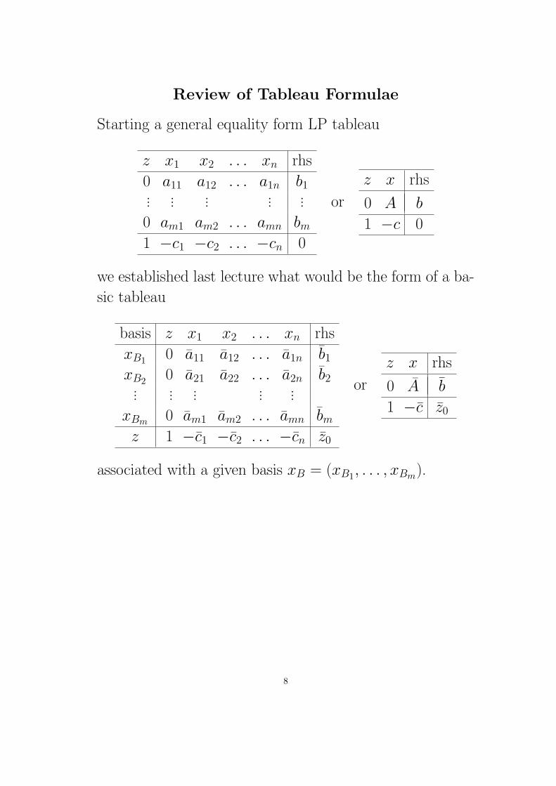
The Artificial Variable Phase I Method
Consider the problem of finding an initial basic feasible
tableau for an LP in standard equality form:
max z = c1x1 + . . . + cnxn
a11x1 + . . . + a1nxn = b1... ...
am1x1 + . . . + amnxn = bm
x1 ≥ 0 . . . xn ≥ 0
A more efficient way to obtain a starting tableau is the
Artificial Phase I Simplex Method. To perform
this method, we first make all of the RHSs nonnegative, by
multiplying each row with negative RHS by -1:
a11x1 + . . . + a1nxn = b1 ≥ 0... ...
am1x1 + . . . + amnxn = bm ≥ 0
x1 ≥ 0 . . . xn ≥ 0
We then add artificial variables to each row of the
tableau:
a11x1 + . . . + a1nxn + xa1 = b1
... ... . . .
am1x1 + . . . + amnxn + xam = bm
x1 ≥ 0, . . . xn ≥ 0, xa1 ≥ 0, . . . xa
m ≥ 0
By using the set of artificial variables as a starting basis,
we obtain a starting basic feasible solution.
2

A feasible solution to the original problem, however, re-
quires that all of the artificial variables equal 0. To
do this we solve a Phase I LP which minimizes the
sum of the artifical variables:
min w = xa1 + . . . + xa
m
a11x1 + . . . + a1nxn + xa1 = b1
... ... . . .
am1x1 + . . . + amnxn + xam = bm
x1 ≥ 0, . . . xn ≥ 0, xa1 ≥ 0, . . . xa
m ≥ 0
This LP always has an optimal solution. (Why?) If its
optimal value w∗ = 0, then the values of the nonartifi-
cial variables will be a feasible solution to the original
LP. If it has optimal value w∗ > 0, then the LP is
infeasible.
Example: Consider the problem given in Lecture 3:
max z = 15x1 − 12x2 − 10x3 − 23x4 + 24x5 + 11x6 − 48x7
4x1 − 3x2 − 2x3 − 6x4 + 8x5 + 3x6 − 9x7 = 164−2x1 + x2 + 4x3 + 4x4 + 2x5 − x6 + x7 = −6612x1 − 4x2 − 6x3 − 13x4 + 9x5 + 4x6 − 7x7 = 272x1 ≥ 0 x2 ≥ 0 x3 ≥ 0 x4 ≥ 0 x5 ≥ 0 x6 ≥ 0 x7 ≥ 0
After negating the second row and adding artificial vari-
ables, we obtain Phase I LP
min w = xa1 + xa
2 + xa3
4x1 − 3x2 − 2x3 − 6x4 + 8x5 + 3x6 − 9x7 + xa1 = 164
2x1 − x2 − 4x3 − 4x4 − 2x5 + x6 − x7 + xa2 = 66
12x1 − 4x2 − 6x3 − 13x4 + 9x5 + 4x6 − 7x7 + xa3 = 272
x1 ≥ 0 x2 ≥ 0 x3 ≥ 0 x4 ≥ 0 x5 ≥ 0 x6 ≥ 0 x7 ≥ 0 xa1 ≥ 0 xa
2 ≥ 0 xa3 ≥ 0
3

Tableaus for the Artificial LP
An artificial LP will have two objective function rows, one
for the artificial LP (to be minimized) and one for the orig-
inal LP (to be maximized).
basis z −w x1 . . . xn xa1 . . . xa
m rhs
xa1 0 0 a11 . . . a1n 1 . . . 0 b1... ... ... ... . . . ... ... ... ...
xam 0 0 am1 . . . amn 0 . . . 1 bm
−w 0 1 0 . . . 0 1 . . . 1 0
z 1 0 −c1 . . . −cn 0 . . . 0 0
We first put the tableau into basic form by costing out
the w row, that is, subtracting each of the first m rows
from the w row:
basis z −w x1 . . . xn xa1 . . . xa
m rhs
xa1 0 0 a11 . . . a1n 1 . . . 0 b1... ... ... ... . . . ... ... ... ...
xam 0 0 am1 . . . amn 0 . . . 1 bm
−w 0 1 −∑mi=1 ai1 . . . −∑m
i=1 ain 0 . . . 0 −∑mi=1 bi
z 1 0 −c1 . . . −cn 0 . . . 0 0
We then proceed to minimize the w-objective (Phase I).
If a feasible solution is found, then the −w row and all
artificial columns are dropped, and we proceed to optimize
the z-objective (Phase II). If a tableau is reached where
the w row reduced costs are all nonnegative, and the RHS
value is still negative, the LP is infeasible.
4

Example
The artificial tableau for our example problem is
basis z −w x1 x2 x3 x4 x5 x6 x7 xa1 xa
2 xa3 rhs
xa1 0 0 4 −3 −2 −6 8 3 −9 1 0 0 164
xa2 0 0 2 −1 −4 −4 −2 1 −1 0 1 0 66
xa3 0 0 12 −4 −6 −13 9 4 −7 0 0 1 272
−w 0 1 0 0 0 0 0 0 0 1 1 1 0
z 1 0 −15 12 10 23 −24 −11 48 0 0 0 0
After costing out the −w row, we get basic feasible artificial
tableau
basis z −w x1 x2 x3 x4 x5 x6 x7 xa1 xa
2 xa3 rhs
xa1 0 0 4 −3 −2 −6 8 3 −9 1 0 0 164
xa2 0 0 2 −1 −4 −4 −2 1 −1 0 1 0 66
xa3 0 0 12 −4 −6 −13 9 4 −7 0 0 1 272
−w 0 1 −18 8 12 23 −15 −8 17 0 0 0 −502
z 1 0 −15 12 10 23 −24 −11 48 0 0 0 0
5

Optimizing with respect to the w row, we pivot first on
the x1 column, third row:
basis z −w x1 x2 x3 x4 x5 x6 x7 xa1 xa
2 xa3 rhs
xa1 0 0 0 −5/3 0 −5/3 5 5/3 −20/3 1 0 −1/3 220/3
xa2 0 0 0 −1/3 −3 −11/6 −7/2 1/3 1/6 0 1 −1/6 62/3
x1 0 0 1 −1/3 −1/2 −13/12 3/4 1/3 −7/12 0 0 1/12 68/3−w 0 1 0 2 3 7/2 −3/2 −2 13/2 0 0 3/2 −94z 1 0 0 7 5/2 27/4 −51/4 −6 157/4 0 0 5/4 340
then in the x6 column, first row:
basis z −w x1 x2 x3 x4 x5 x6 x7 xa1 xa
2 xa3 rhs
x6 0 0 0 −1 0 −1 3 1 −4 3/5 0 −1/5 44xa
1 0 0 0 0 −3 −3/2 −9/2 0 3/2 −1/5 1 −1/10 6x1 0 0 1 0 −1/2 −3/4 −1/4 0 3/4 −1/5 0 3/20 8−w 0 1 0 0 3 3/2 9/2 0 −3/2 6/5 0 11/10 −6z 1 0 0 1 5/2 3/4 21/4 0 61/4 18/5 0 1/20 604
and finally, on the x7 column, second row:
basis z −w x1 x2 x3 x4 x5 x6 x7 xa1 xa
2 xa3 rhs
x6 0 0 0 −1 −8 −5 −9 1 0 1/15 8/3 −7/15 60x7 0 0 0 0 −2 −1 −3 0 1 −2/15 2/3 −1/15 4x1 0 0 1 0 1 0 2 0 0 −1/10 −1/2 1/5 5−w 0 1 0 0 0 0 0 0 0 1 1 1 0z 1 0 0 1 33 16 51 0 0 169/30 −61/6 16/15 543
The w objective is now minimized at 0, and the basis is
now feasible, with feasible solution x1 = 5, x2 = x3 = x4 =
x5 = 0, x6 = 60, and x7 = 4. Dropping the w row and
the three artificial columns, we see that the current solution
is also optimal, and so Phase II has produced an optimal
tableau.
6

If we change the original RHS of the original LP to 184,
-106, and 332, we get starting basic feasible tableau
basis z −w x1 x2 x3 x4 x5 x6 x7 xa1 xa
2 xa3 rhs
xa1 0 0 4 −3 −2 −6 8 3 −9 1 0 0 184
xa2 0 0 2 −1 −4 −4 −2 1 −1 0 1 0 106
xa3 0 0 12 −4 −6 −13 9 4 −7 0 0 1 332
−w 0 1 −18 8 12 23 −15 −8 17 0 0 0 −622
z 1 0 −15 12 10 23 −24 −11 48 0 0 0 0
We take the same first two pivots, resulting in tableau
basis z −w x1 x2 x3 x4 x5 x6 x7 xa1 xa
2 xa3 rhs
x6 0 0 0 −1 0 −1 3 1 −4 3/5 0 −1/5 44xa
2 0 0 0 0 −3 −3/2 −9/2 0 3/2 −1/5 1 −1/10 36x1 0 0 1 0 −1/2 −3/4 −1/4 0 3/4 −1/5 0 3/20 13−w 0 1 0 0 3 3/2 9/2 0 −3/2 6/5 0 11/10 −36z 1 0 0 1 5/2 3/4 21/4 0 61/4 18/5 0 1/20 679
Now a pivot in the x7 column must be done in the thirdrow, resulting in tableau
basis z −w x1 x2 x3 x4 x5 x6 x7 xa1 xa
2 xa3 rhs
x6 0 0 16/3 −1 −8/3 −5 5/3 1 0 −7/15 0 3/5 340/3xa
2 0 0 −2 0 −2 0 −4 0 0 1/5 1 −2/5 10x7 0 0 4/3 0 −2/3 −1 −1/3 0 1 −4/15 0 1/5 52/3−w 0 1 2 0 2 0 4 0 0 4/5 0 7/5 −10z 1 0 −61/3 1 38/3 16 31/3 0 0 23/3 0 −3 1244/3
The optimal value of w is 10 > 0, and so the original LP is
infeasible.
7
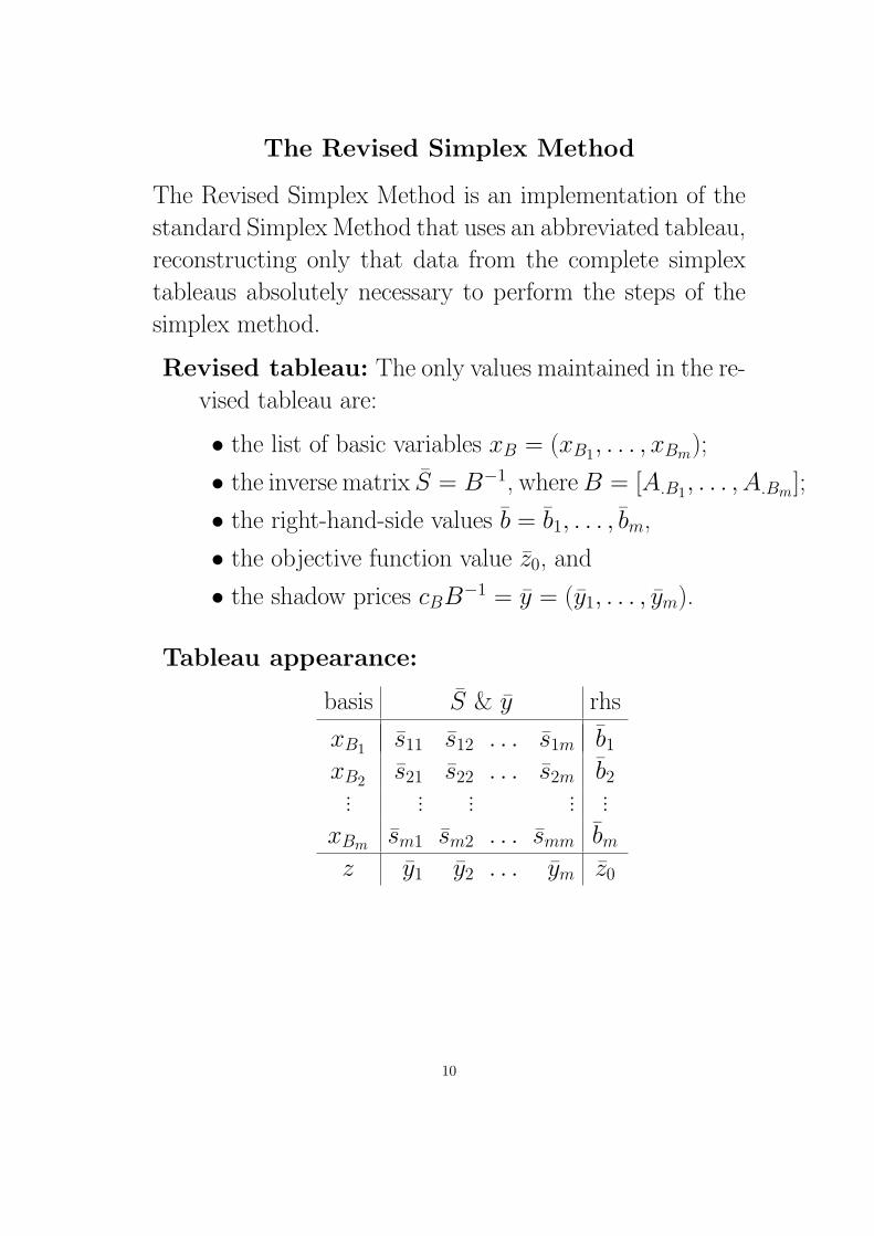
Review of Tableau Formulae
Starting a general equality form LP tableau
z x1 x2 . . . xn rhs
0 a11 a12 . . . a1n b1... ... ... ... ...
0 am1 am2 . . . amn bm
1 −c1 −c2 . . . −cn 0
or
z x rhs
0 A b
1 −c 0
we established last lecture what would be the form of a ba-
sic tableau
basis z x1 x2 . . . xn rhs
xB1 0 a11 a12 . . . a1n b1
xB2 0 a21 a22 . . . a2n b2... ... ... ... ...
xBm 0 am1 am2 . . . amn bm
z 1 −c1 −c2 . . . −cn z0
or
z x rhs
0 A b
1 −c z0
associated with a given basis xB = (xB1, . . . , xBm).
8

Simply partition the columns of the tableau into basic
and nonbasic variables
z xB xN rhs
0 B N b
1 −cB −cN 0
and set shadow prices and basis inverse to
y = cBB−1 and S = B−1 =
s11 . . . s1m... ...
sm1 . . . smm
Then the tableau can be written
basis z x rhs
xB 0 A b
z 1 −c z0
=
basis z x rhs
xB 0 SA Sb
z 1 −c + yA yb
with associated formulae
(1) aij = si1a1j + si2a2j + . . . + simamji = 1, . . . , mj = 1, . . . , n
(2) bi = si1b1 + si2b2 + . . . + simbm i = 1, . . . , m
(3) cj = cj − y1a1j − y2a2j − . . .− ymamj j = 1, . . . , n
(4) z0 = y1b1 + y2b2 + . . . + ymbm
9
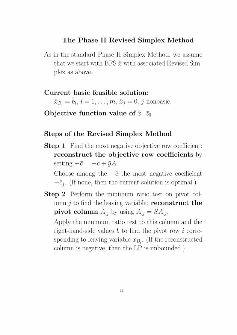
The Revised Simplex Method
The Revised Simplex Method is an implementation of the
standard Simplex Method that uses an abbreviated tableau,
reconstructing only that data from the complete simplex
tableaus absolutely necessary to perform the steps of the
simplex method.
Revised tableau: The only values maintained in the re-
vised tableau are:
• the list of basic variables xB = (xB1, . . . , xBm);
• the inverse matrix S = B−1, where B = [A.B1, . . . , A.Bm];
• the right-hand-side values b = b1, . . . , bm,
• the objective function value z0, and
• the shadow prices cBB−1 = y = (y1, . . . , ym).
Tableau appearance:
basis S & y rhs
xB1 s11 s12 . . . s1m b1
xB2 s21 s22 . . . s2m b2... ... ... ... ...
xBm sm1 sm2 . . . smm bm
z y1 y2 . . . ym z0
10
The Phase II Revised Simplex Method
As in the standard Phase II Simplex Method, we assume
that we start with BFS x with associated Revised Sim-
plex as above.
Current basic feasible solution:
xBi= bi, i = 1, . . . , m, xj = 0, j nonbasic.
Objective function value of x: z0
Steps of the Revised Simplex Method
Step 1 Find the most negative objective row coefficient:
reconstruct the objective row coefficients by
setting −c = −c + yA.
Choose among the −c the most negative coefficient
−cj. (If none, then the current solution is optimal.)
Step 2 Perform the minimum ratio test on pivot col-
umn j to find the leaving variable: reconstruct the
pivot column A.j by using A.j = SA.j.
Apply the minimum ratio test to this column and the
right-hand-side values b to find the pivot row i corre-
sponding to leaving variable xBi. (If the reconstructed
column is negative, then the LP is unbounded.)
11

Step 3 Perform a pivot on row i and column j: insert
reconstructed column j next to the inverse matrix
and perform a pivot on the associated row, replacing
the blocking variable xBiwith the entering variable xj.
The updated values of S, b, z, and y are then the cor-
rect ones for the new basis.
basis S & y xj rhs
xB1 s11 . . . s1m a1j b1... ... ... ... ...
xBisi1 . . . sim aij bi
... ... ... ... ...
xBm sm1 . . . smm amj bm
z y1 . . . ym −cj z0
12
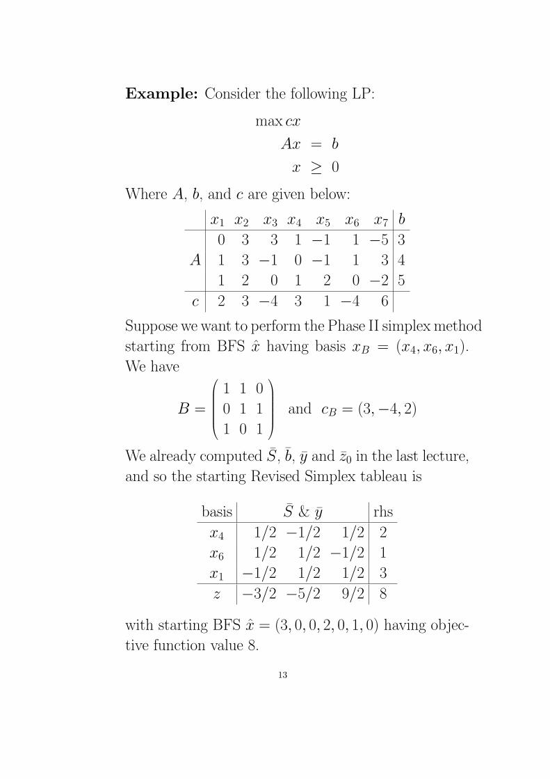
Example: Consider the following LP:
max cx
Ax = b
x ≥ 0
Where A, b, and c are given below:
x1 x2 x3 x4 x5 x6 x7 b
0 3 3 1 −1 1 −5 3
A 1 3 −1 0 −1 1 3 4
1 2 0 1 2 0 −2 5
c 2 3 −4 3 1 −4 6
Suppose we want to perform the Phase II simplex method
starting from BFS x having basis xB = (x4, x6, x1).
We have
B =
1 1 0
0 1 1
1 0 1
and cB = (3,−4, 2)
We already computed S, b, y and z0 in the last lecture,
and so the starting Revised Simplex tableau is
basis S & y rhs
x4 1/2 −1/2 1/2 2
x6 1/2 1/2 −1/2 1
x1 −1/2 1/2 1/2 3
z −3/2 −5/2 9/2 8
with starting BFS x = (3, 0, 0, 2, 0, 1, 0) having objec-
tive function value 8.
13

Iteration 1: We have
−c = −(2, 3,−4, 3, 1,−4, 6) + (−3/2,−5/2, 9/2)
0 3 3 1 −1 1 −51 3 −1 0 −1 1 31 2 0 1 2 0 −2
= (0,−6, 2, 0, 12, 0,−15)
The most negative is the −c7 = −15 term, and so we
reconstruct column A.7:
A.7 =
1/2 −1/2 1/2
1/2 1/2 −1/2
−1/2 1/2 1/2
−5
3
−2
=
−5
0
3
The leaving variable is now xB3 = x1, and so we pivot
on tableau
basis S & y x7 rhs
x4 1/2 −1/2 1/2 −5 2
x6 1/2 1/2 −1/2 0 1
x1 −1/2 1/2 1/2 3 3
z −3/2 −5/2 9/2 −15 8
to give new revised tableau
basis S & y rhs
x4 −1/3 1/3 4/3 7
x6 1/2 1/2 −1/2 1
x7 −1/6 1/6 1/6 1
z −4 0 7 23
with current BFS x = (0, 0, 0, 7, 0, 1, 1) having objec-
tive function value 23.
14

Iteration 2: We have
−c = −(2, 3,−4, 3, 1,−4, 6) + (−4, 0, 7)
0 3 3 1 −1 1 −51 3 −1 0 −1 1 31 2 0 1 2 0 −2
= (5,−1,−8, 0, 17, 0, 0)
The most negative is the −c3 = −8 term, and so we
reconstruct the A.3 column
A.3 =
−1/3 1/3 4/3
1/2 1/2 −1/2
−1/6 1/6 1/6
3
−1
0
=
−4/3
1
−2/3
The leaving variable is now xB2 = x6, and so we pivot
on tableau
basis S & y x3 rhs
x4 −1/3 1/3 4/3 −4/3 7
x6 1/2 1/2 −1/2 1 1
x7 −1/6 1/6 1/6 −2/3 1
z −4 0 7 −8 23
to give new revised tableau
basis S & y rhs
x4 1/3 1 2/3 25/3
x3 1/2 1/2 −1/2 1
x7 1/6 1/2 −1/6 5/3
z 0 4 3 31
with current BFS x = (0, 0, 1, 813, 0, 0, 1
23) having ob-
jective function value 31.
15

Iteration 3: We have
−c = −(2, 3,−4, 3, 1,−4, 6) + (0, 4, 3)
0 3 3 1 −1 1 −51 3 −1 0 −1 1 31 2 0 1 2 0 −2
= (5, 15, 0, 0, 1, 8, 0)
Since all reduced costs are nonnegative, the current
solution is optimal to the LP.
16

Comments on Revised Simplex Method
• Revised tableau is only of size O(m2), as opposed
to O(mn) for the standard tableau. This means
that the pivot step, which is most expensive, takes
only O(m2) time, rather than O(mn).
• In implementation, the Revised Simplex Method
does not keep B−1 around at all, but simply keeps
the basis matrix B and solves Bx = b to find b,
xB = cB to find y, etc. Thus it can take advantage
of sparsity of matrices, and use sophisticated tech-
niques like LU decomposition or iterative methods
to obtain fast solutions or approximations to the
values required to perform a simplex pivot.
• One of the most expensive steps is the generation
of the reduced costs. This can be improved by
generating a large number of negative reduced cost
columns at once, and then performing simplex piv-
ots on these columns, where appropriate, without
regenerating the reduced costs before every pivot.
• The Revised Simplex Method is particularly effec-
tive for delayed column generation techniques,
where the number of columns is so prohibitively
large that they must be generated one at a time,
rather than all at once at the beginning. More on
this later in the course.
17
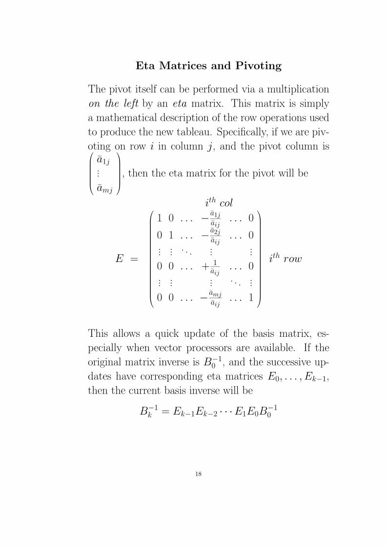
Eta Matrices and Pivoting
The pivot itself can be performed via a multiplication
on the left by an eta matrix. This matrix is simply
a mathematical description of the row operations used
to produce the new tableau. Specifically, if we are piv-
oting on row i in column j, and the pivot column is
a1j...
amj
, then the eta matrix for the pivot will be
ith col
E =
1 0 . . . − a1j
aij. . . 0
0 1 . . . − a2j
aij. . . 0
... ... . . . ... ...
0 0 . . . + 1aij
. . . 0... ... ... . . . ...
0 0 . . . − amj
aij. . . 1
ith row
This allows a quick update of the basis matrix, es-
pecially when vector processors are available. If the
original matrix inverse is B−10 , and the successive up-
dates have corresponding eta matrices E0, . . . , Ek−1,
then the current basis inverse will be
B−1k = Ek−1Ek−2 · · ·E1E0B
−10
18
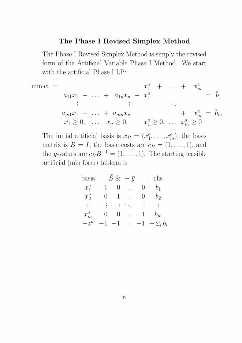
The Phase I Revised Simplex Method
The Phase I Revised Simplex Method is simply the revised
form of the Artificial Variable Phase I Method. We start
with the artificial Phase I LP:
min w = xa1 + . . . + xa
m
a11x1 + . . . + a1nxn + xa1 = b1
... ... . . .
am1x1 + . . . + amnxn + xam = bm
x1 ≥ 0, . . . xn ≥ 0, xa1 ≥ 0, . . . xa
m ≥ 0
The initial artificial basis is xB = (xa1, . . . , x
am), the basis
matrix is B = I , the basic costs are cB = (1, . . . , 1), and
the y-values are cBB−1 = (1, . . . , 1). The starting feasible
artificial (min form) tableau is
basis S & − y rhs
xa1 1 0 . . . 0 b1
xa2 0 1 . . . 0 b2... ... ... . . . ... ...
xam 0 0 . . . 1 bm
−za −1 −1 . . . −1 −∑i bi
19

We now proceed to apply the Phase II Simplex Method
— using the artificial cost vector (0, . . . , 0, 1, . . . , 1) —
until an optimal solution is reached. If all of the artificial
variables are 0, then the current solution is feasible to the
original LP. We now only need to replace the artificial y
and z0 values with their values for the original LP:
y = cBB−1, z0 = cBB−1b
to obtain the correct starting revised tableau for the Phase
II. We then proceed with the standard Phase II simplex
method, using the original objective function for the re-
duced cost computations (which do not include any of the
artificial variables), until either an optimal solution is found
or the LP is determined to be unbounded.
Example: Consider the problem of finding an initial ba-
sic feasible solution to the problem above. The artifical
LP for this problem is:
x1 x2 x3 x4 x5 x6 x7 xa1 xa
2 xa3 b
0 3 3 1 −1 1 −5 1 0 0 3
Aa 1 3 −1 0 −1 1 3 0 1 0 4
1 2 0 1 2 0 −2 0 0 1 5
ca 0 0 0 0 0 0 0 1 1 1
The starting artificial revised tableau for this is
basis S & − y rhs
xa1 1 0 0 3
xa2 0 1 0 4
xa3 0 0 1 5
−za −1 −1 −1 −12
20

Iteration 1:
c = (0, 0, 0, 0, 0, 0, 0, 1, 1, 1)− (1, 1, 1)
0 3 3 1 −1 1 −5 1 0 01 3 −1 0 −1 1 3 0 1 01 2 0 1 2 0 −2 0 0 1
= (−2,−8,−2,−2, 0,−2, 4, 0, 0, 0)
x2 enters, with pivot column
A.2 =
1 0 0
0 1 0
0 0 1
3
3
2
=
3
3
2
The leaving variable is xa1, and the resulting tableau is
basis S & − y rhs
x2 1/3 0 0 1
xa2 −1 1 0 1
xa3 −2/3 0 1 3
−za 5/3 −1 −1 −4
Iteration 2:
c = (0, 0, 0, 0, 0, 0, 0, 1, 1, 1)− (−5/3, 1, 1)
0 3 3 1 −1 1 −5 1 0 01 3 −1 0 −1 1 3 0 1 01 2 0 1 2 0 −2 0 0 1
= (−2, 0, 6, 2/3,−8/3, 2/3,−28/3, 8/3, 0, 0)
x7 enters, with pivot column
A.7 =
1/3 0 0
−1 1 0
−2/3 0 1
−5
3
−2
=
−5/3
8
4/3
21

The leaving variable is xa2, and the resulting tableau is
basis S & − y rhs
x2 1/8 5/24 0 29/24
x7 −1/8 −1/8 0 1/8
xa3 −1/2 1/6 1 17/6
−za 1/2 1/6 −1 −17/6
Iteration 3:
c = (0, 0, 0, 0, 0, 0, 0, 1, 1, 1)− (−1/2,−1/6, 1)
0 3 3 1 −1 1 −5 1 0 01 3 −1 0 −1 1 3 0 1 01 2 0 1 2 0 −2 0 0 1
= (−5/6, 0, 4/3,−1/2,−8/3, 2/3, 0, 3/2, 7/6, 0)
x5 enters, with pivot column
A.5 =
1/8 5/24 0
−1/8 −1/8 0
−1/2 1/6 1
−1
−1
2
=
−1/3
0
8/3
The leaving variable is xa3, and the resulting tableau is
basis S & − y rhs
x2 1/16 3/16 1/8 25/16
x7 −1/8 1/8 0 1/8
x5 −3/16 −1/16 3/8 17/6
−za 0 0 0 0
22
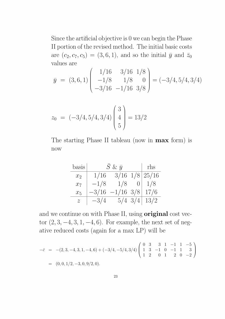
Since the artificial objective is 0 we can begin the Phase
II portion of the revised method. The initial basic costs
are (c2, c7, c5) = (3, 6, 1), and so the initial y and z0
values are
y = (3, 6, 1)
1/16 3/16 1/8
−1/8 1/8 0
−3/16 −1/16 3/8
= (−3/4, 5/4, 3/4)
z0 = (−3/4, 5/4, 3/4)
3
4
5
= 13/2
The starting Phase II tableau (now in max form) is
now
basis S & y rhs
x2 1/16 3/16 1/8 25/16
x7 −1/8 1/8 0 1/8
x5 −3/16 −1/16 3/8 17/6
z −3/4 5/4 3/4 13/2
and we continue on with Phase II, using original cost vec-
tor (2, 3,−4, 3, 1,−4, 6). For example, the next set of neg-
ative reduced costs (again for a max LP) will be
−c = −(2, 3,−4, 3, 1,−4, 6) + (−3/4,−5/4, 3/4)
0 3 3 1 −1 1 −51 3 −1 0 −1 1 31 2 0 1 2 0 −2
= (0, 0, 1/2,−3, 0, 9/2, 0).
23
Top Related