


Languages
Pages
Legal


Integrated Quality and Quantity Modelling
of a Production Line
by
Jongyoon Kim
B.S., Seoul National University (1997)M.S., Seoul National University (1999)
Submitted to the Department of Mechanical Engineeringin partial fulfillment of the requirements for the degree of
Doctor of Philosophy in Mechanical Engineering
at the
MASSACHUSETTS INSTITUTE OF TECHNOLOGY
February 2005
c© Massachusetts Institute of Technology 2005. All rights reserved.
Author . . . . . . . . . . . . . . . . . . . . . . . . . . . . . . . . . . . . . . . . . . . . . . . . . . . . . . . . . . . . . .Department of Mechanical Engineering
November 10, 2004
Certified by. . . . . . . . . . . . . . . . . . . . . . . . . . . . . . . . . . . . . . . . . . . . . . . . . . . . . . . . . .Stanley B. Gershwin
Senior Research ScientistThesis Supervisor
Accepted by . . . . . . . . . . . . . . . . . . . . . . . . . . . . . . . . . . . . . . . . . . . . . . . . . . . . . . . . .Lallit Anand
Chairman, Department Committee on Graduate Students

2

Integrated Quality and Quantity Modelling
of a Production Line
by
Jongyoon Kim
Submitted to the Department of Mechanical Engineeringon November 10, 2004, in partial fulfillment of the
requirements for the degree ofDoctor of Philosophy in Mechanical Engineering
Abstract
The interaction of quantity and quality performance in a factory is clearly of greateconomic importance. However, there is very little quantitative analytical literaturein this area. This thesis is an essential early research step in analyzing how productionsystem design, quality, and productivity are inter-related in transfer lines. We developa new Markov process model for machines with both quality and operational failures,and we identify important differences between types of quality failures. We presentanalytic models, solution techniques, performance evaluations, and validation of two-machine systems as well as longer transfer lines. Through numerical studies, wehave investigated some of the conventional wisdom on this interaction, and we havefound that the wisdom holds only under specific conditions, and we show that theconventional wisdom is wrong under other conditions. We therefore anticipate thatmore such research will have a dramatic effect on the performance of factories, andwe propose promising research directions.
Thesis Supervisor: Stanley B. GershwinTitle: Senior Research Scientist
3

4

Acknowledgments
Not only does this dissertation mark the end of a considerable academic endeavor
(twenty-three years of formal education), but it also represents a personal success
that could not have been realized without the support of many individuals along the
way. The thanks and gratitude I offer to these people is authentic and well-deserved.
First and foremost, I wish to thank my family for the love and support that they
have given me. I am forever indebted to my parents, Moogon Kim and Dukhee Jeon,
for their affection and unending patience throughout my life. I would like to thank
my loving wife, Sooyeon Hwang. It was her encouragement, hope, and belief in me
and my ideas that kept me going when I struggled. I am so grateful to have my son
Ryan. I truly believe that he is the biggest achievement and the greatest source of
happiness in my life. To my sisters, Moonjung and Hyunjung, my gratitude for the
wonderful time we spent in my childhood.
Many professors helped make this possible, but none more than my advisor, Dr.
Stanley B. Gershwin. His passion about manufacturing systems engineering is extra-
ordinary, as are the breadth and depth of his thinking. Thank you, Stan, you have
been a wonderful academic advisor, mentor, and friend to me. I would like to thank
Professor David Hardt and Professor Duane Boning for serving on my thesis commit-
tee. Their valuable advice and continuous support helped me to complete this work.
I would also like to extend my thanks to other professors who were fundamental to
my education. Professor Gutowski, thank you for giving me an opportunity to be a
TA of Course 2.810. To Professor Hyo-Chol Sin of Seoul National Univeristy, I say:
You were right; MIT is the greatest place to be for the highest level of education and
research. I appreciate your helping me to come to MIT. Special thanks also to my
high school math teacher Changwon Lee, who taught me the beauty of mathematics.
The students I have shared many days and nights with have also been extraor-
dinary. To my lab mates at the Manufacturing Systems Lab and the Production
Systems Design Lab, Yong-Suk Kim, Jochen Link, Chiwon Kim, Youngjae Jang,
Zhenwei Zhao, Zhenyu Zhang, Quinton Ng, Jim Duda, Jorge Arinez, Jose Casteneda-
Vega, and Carlos Tapia: Thank you. In addition, I would like to express my gratitude
to the officers of Korean Graduate Student Association (KGSA) at MIT, who made
me a successful president. MIT KGSA squash team members, Kyungyoon Noh,
Hyungsuk Lee, and Kyujin Cho, I do not forget the moment when we got the first
place at MIT Intramural Squash Competition in 2001. Daekeun Kim and Taesik Lee,
5

I really enjoyed drinking with you in the Chinatown. My best friends Youngjoo Lee
and Jungjae Cho, you guys are incredible.
None of this work would have been possible were it not for the generous financial
support from General Motors, PSA Peugeot-Citron, Ford Motors, and MIT-Singapore
alliance. Special thanks to Alain Patchong from PSA Peugeot-Citron, Jingshan Li
and Dennis Blumenfeld from General Motors. There is no question that I learned a
great deal about the world of manufacturing from all of you.
Finally, Boston Redsox, who won the world series in 2004, you gave me incredible
amount of excitement while I have stayed in Boston. Yes we are the champion!
6

Contents
1 Introduction 17
1.1 Motivation . . . . . . . . . . . . . . . . . . . . . . . . . . . . . . . . . 17
1.2 Background and literature review . . . . . . . . . . . . . . . . . . . . 19
1.2.1 Importance of quality . . . . . . . . . . . . . . . . . . . . . . . 19
1.2.2 Quality models . . . . . . . . . . . . . . . . . . . . . . . . . . 19
1.2.3 System yield . . . . . . . . . . . . . . . . . . . . . . . . . . . . 21
1.2.4 Quality improvement strategy . . . . . . . . . . . . . . . . . . 21
1.2.5 Lean manufacturing, people, and quality . . . . . . . . . . . . 22
1.2.6 Stochastic modeling of manufacturing systems . . . . . . . . . 23
1.3 Thesis Outline . . . . . . . . . . . . . . . . . . . . . . . . . . . . . . . 24
2 Fundamental Models 25
2.1 Taxonomy and modeling assumptions . . . . . . . . . . . . . . . . . . 25
2.1.1 Definition of terminology . . . . . . . . . . . . . . . . . . . . . 25
2.1.2 Modeling assumptions . . . . . . . . . . . . . . . . . . . . . . 29
2.2 Single machine model . . . . . . . . . . . . . . . . . . . . . . . . . . . 30
2.3 Simulation Model . . . . . . . . . . . . . . . . . . . . . . . . . . . . . 33
2.4 Special two-machine-one-buffer (2M1B) model . . . . . . . . . . . . . 34
2.4.1 Infinite buffer case . . . . . . . . . . . . . . . . . . . . . . . . 34
2.4.2 Zero buffer case . . . . . . . . . . . . . . . . . . . . . . . . . . 34
3 Two-Machine-One-Finite-Buffer (2M1B) Line 37
3.1 Modeling . . . . . . . . . . . . . . . . . . . . . . . . . . . . . . . . . . 37
3.1.1 State definition . . . . . . . . . . . . . . . . . . . . . . . . . . 37
3.1.2 Internal Transition Equations . . . . . . . . . . . . . . . . . . 38
3.1.3 Boundary transition equations . . . . . . . . . . . . . . . . . . 40
3.1.4 Normalization . . . . . . . . . . . . . . . . . . . . . . . . . . . 47
7

3.1.5 Performance measures . . . . . . . . . . . . . . . . . . . . . . 48
3.2 Solution technique . . . . . . . . . . . . . . . . . . . . . . . . . . . . 49
3.2.1 Solution to internal transition equations . . . . . . . . . . . . 49
3.2.2 Algorithm to solve equations (3.138) and (3.139) . . . . . . . . 53
3.2.3 Building the probability density function . . . . . . . . . . . . 71
3.2.4 Methods to solve boundary conditions . . . . . . . . . . . . . 72
3.2.5 Methods to evaluate performance measures . . . . . . . . . . . 78
3.3 Validation . . . . . . . . . . . . . . . . . . . . . . . . . . . . . . . . . 80
3.4 Quality information feedback . . . . . . . . . . . . . . . . . . . . . . 82
4 Insights From Numerical Experimentation 87
4.1 Beneficial buffer case . . . . . . . . . . . . . . . . . . . . . . . . . . . 87
4.1.1 Production rates . . . . . . . . . . . . . . . . . . . . . . . . . 87
4.1.2 System yield and buffer size . . . . . . . . . . . . . . . . . . . 89
4.2 Harmful buffer case . . . . . . . . . . . . . . . . . . . . . . . . . . . . 89
4.2.1 Production rates . . . . . . . . . . . . . . . . . . . . . . . . . 89
4.2.2 System Yield . . . . . . . . . . . . . . . . . . . . . . . . . . . 90
4.3 Optimal buffer case . . . . . . . . . . . . . . . . . . . . . . . . . . . . 91
4.4 How to improve quality in a line with
persistent quality failures . . . . . . . . . . . . . . . . . . . . . . . . . 93
4.5 How to increase the effective production rate . . . . . . . . . . . . . . 95
5 Long Line Analysis 97
5.1 Introduction . . . . . . . . . . . . . . . . . . . . . . . . . . . . . . . . 97
5.1.1 Approximation techniques in long line analysis . . . . . . . . . 97
5.1.2 Decomposition techniques for continuous models
without quality failures . . . . . . . . . . . . . . . . . . . . . . 98
5.2 Long line analysis case 1 . . . . . . . . . . . . . . . . . . . . . . . . . 101
5.2.1 Introduction . . . . . . . . . . . . . . . . . . . . . . . . . . . . 101
5.2.2 Solution method . . . . . . . . . . . . . . . . . . . . . . . . . 102
5.2.3 Performance Evaluation . . . . . . . . . . . . . . . . . . . . . 107
5.3 Long Line Analysis Case 2 . . . . . . . . . . . . . . . . . . . . . . . . 109
5.3.1 Introduction . . . . . . . . . . . . . . . . . . . . . . . . . . . . 109
5.3.2 Solution method . . . . . . . . . . . . . . . . . . . . . . . . . 110
5.3.3 Performance Evaluation . . . . . . . . . . . . . . . . . . . . . 111
8

5.4 Long Line Analysis Case 3 . . . . . . . . . . . . . . . . . . . . . . . . 113
5.4.1 Introduction . . . . . . . . . . . . . . . . . . . . . . . . . . . . 113
5.4.2 Solution method . . . . . . . . . . . . . . . . . . . . . . . . . 114
5.4.3 Performance Evaluation . . . . . . . . . . . . . . . . . . . . . 116
6 Jidoka 119
6.1 Jidoka practice in Toyota Production System . . . . . . . . . . . . . . 119
6.2 Modeling of Multiple-Yield Quality Failures . . . . . . . . . . . . . . 121
6.2.1 Multiple-Yield Quality Failures . . . . . . . . . . . . . . . . . 121
6.2.2 Modeling of Stopping Policies . . . . . . . . . . . . . . . . . . 123
6.2.3 Optimality of stopping with one defect . . . . . . . . . . . . . 125
7 Future Research 131
7.1 Two-machine-one-buffer systems . . . . . . . . . . . . . . . . . . . . . 131
7.1.1 Part scrapping at each operation . . . . . . . . . . . . . . . . 131
7.1.2 Part rework . . . . . . . . . . . . . . . . . . . . . . . . . . . . 132
7.1.3 Correlation among different quality failures . . . . . . . . . . . 132
7.1.4 Reliability of inspection . . . . . . . . . . . . . . . . . . . . . 132
7.1.5 Productivity reduction due to inspection . . . . . . . . . . . . 133
7.1.6 Aging . . . . . . . . . . . . . . . . . . . . . . . . . . . . . . . 133
7.2 Large systems . . . . . . . . . . . . . . . . . . . . . . . . . . . . . . . 134
7.2.1 Topology of manufacturing systems . . . . . . . . . . . . . . . 134
7.2.2 Location and domain of inspection . . . . . . . . . . . . . . . 134
7.2.3 Behavior of long lines . . . . . . . . . . . . . . . . . . . . . . . 135
7.3 Optimal manufacturing system design . . . . . . . . . . . . . . . . . 136
7.4 Worker motivation and learning . . . . . . . . . . . . . . . . . . . . . 137
8 Conclusion 139
A 2M1B parameters 151
B Long Line Task Parameters 161
B.1 Ubiquitous inspection case . . . . . . . . . . . . . . . . . . . . . . . . 161
B.2 Extended quality information feedback case . . . . . . . . . . . . . . 166
B.3 Multiple quality information feedback case . . . . . . . . . . . . . . . 171
C Matrix manipulation technique 177
9

10

List of Figures
1-1 Types of Quality Failures . . . . . . . . . . . . . . . . . . . . . . . . . 20
2-1 Five-Machine Flow Line . . . . . . . . . . . . . . . . . . . . . . . . . 25
2-2 Two-Machine-One-Buffer Continuous Model . . . . . . . . . . . . . . 27
2-3 States of a Machine . . . . . . . . . . . . . . . . . . . . . . . . . . . 31
2-4 States of a Generalized Machine . . . . . . . . . . . . . . . . . . . . 32
3-1 Two-machine-one-buffer line . . . . . . . . . . . . . . . . . . . . . . . 37
3-2 Plot of Equations (3.138) and (3.139) . . . . . . . . . . . . . . . . . . 54
3-3 Typical shape of the solutions of equations 3.138 and 3.139 . . . . . . 58
3-4 Plot of the simplified internal transition equations with µ1 > µ2 . . . 59
3-5 Plot of the simplified internal transition equations with µ1 = µ2 . . . 59
3-6 Plot of the simplified internal transition equations with µ1 < µ2 . . . 59
3-7 Root finding in region 1 . . . . . . . . . . . . . . . . . . . . . . . . . 60
3-8 Plot of red lines and blue lines with µ1 < µ2 in region 2 . . . . . . . . 61
3-9 Case 1 and Case 2 . . . . . . . . . . . . . . . . . . . . . . . . . . . . 62
3-10 Case 3 and Case 4 . . . . . . . . . . . . . . . . . . . . . . . . . . . . 62
3-11 Case 5 and Case 6 . . . . . . . . . . . . . . . . . . . . . . . . . . . . 62
3-12 Case 7 and Case 8 . . . . . . . . . . . . . . . . . . . . . . . . . . . . 63
3-13 Case 9 and Case 10 . . . . . . . . . . . . . . . . . . . . . . . . . . . . 63
3-14 Case 11 and Case 12 . . . . . . . . . . . . . . . . . . . . . . . . . . . 64
3-15 Case 13 and Case 14 . . . . . . . . . . . . . . . . . . . . . . . . . . . 65
3-16 Case 15 and Case 16 . . . . . . . . . . . . . . . . . . . . . . . . . . . 66
3-17 Plot of red lines and blue lines with µ1 > µ2 in region 4 . . . . . . . . 66
3-18 Case 1 and Case 2 . . . . . . . . . . . . . . . . . . . . . . . . . . . . 67
3-19 Case 3 and Case 4 . . . . . . . . . . . . . . . . . . . . . . . . . . . . 67
3-20 Case 5 and Case 6 . . . . . . . . . . . . . . . . . . . . . . . . . . . . 68
11

3-21 Case 7 and Case 8 . . . . . . . . . . . . . . . . . . . . . . . . . . . . 68
3-22 Case 9 and Case 10 . . . . . . . . . . . . . . . . . . . . . . . . . . . . 69
3-23 Case 11 and Case 12 . . . . . . . . . . . . . . . . . . . . . . . . . . . 69
3-24 Case 13 and Case 14 . . . . . . . . . . . . . . . . . . . . . . . . . . . 70
3-25 Case 15 and Case 16 . . . . . . . . . . . . . . . . . . . . . . . . . . . 71
3-26 Validation of the total production rate . . . . . . . . . . . . . . . . . 80
3-27 Validation of the effective production rate . . . . . . . . . . . . . . . 81
3-28 Validation of average inventory . . . . . . . . . . . . . . . . . . . . . 81
3-29 Quality information feedback: total production rate . . . . . . . . . . 85
3-30 Quality information feedback: effective production rate . . . . . . . . 85
3-31 Quality information feedback: average inventory . . . . . . . . . . . . 85
4-1 Beneficial Buffer Case: Total Production Rate . . . . . . . . . . . . . 88
4-2 Beneficial Buffer Case: Effective Production Rate . . . . . . . . . . . 88
4-3 Beneficial Buffer Case: System Yield as a Function of Buffer Size . . 89
4-4 Harmful Buffer Case: Effective Production Rate . . . . . . . . . . . . 90
4-5 Harmful Buffer Case: Total Production Rate . . . . . . . . . . . . . . 91
4-6 Harmful Buffer Case: System Yield as a Function of Buffer Size . . . 91
4-7 Optimal Buffer Size Case: Effective Production Rate . . . . . . . . . 92
4-8 Optimal Buffer Size Case: Total Production Rate . . . . . . . . . . . 92
4-9 Optimal Buffer Size Case: System Yield . . . . . . . . . . . . . . . . 93
4-10 Quality Improvement Through Increase of MTQF . . . . . . . . . . . 94
4-11 Quality Improvement Through Increase of f . . . . . . . . . . . . . . 94
4-12 Mean Time to Detect and Effective Production Rate . . . . . . . . . 95
4-13 Quality Failure Frequency and Effective Production Rate . . . . . . . 96
5-1 Decomposition of a four-machine line into three two-machine lines . . 99
5-2 The first long line analysis task . . . . . . . . . . . . . . . . . . . . . 102
5-3 Three-state-machine and corresponding two-state-machine . . . . . . 103
5-4 Distribution of transition time from up states to down state: three-
state machines . . . . . . . . . . . . . . . . . . . . . . . . . . . . . . . 105
5-5 3-state-machine vs. 2-state-machine - comparison of PT . . . . . . . 106
5-6 3-state-machine vs. 2-state-machine - comparison of PE . . . . . . . 106
5-7 3-state-machine vs. 2-state-machine - comparison of Inv . . . . . . . 106
5-8 Validation – total production rate and effective production rate . . . 108
12
5-9 Validation – WIP (Work-In-Process) and average inventory at B1 . . 108
5-10 Validation – average inventory at B2 and B3 . . . . . . . . . . . . . . 109
5-11 The second long line analysis task . . . . . . . . . . . . . . . . . . . . 109
5-12 Procedure of long line analysis task 2 . . . . . . . . . . . . . . . . . . 111
5-13 Validation - PT and PE . . . . . . . . . . . . . . . . . . . . . . . . . . 112
5-14 Validation - WIP and Average Inventory at B1 . . . . . . . . . . . . 112
5-15 Validation - Average Inventory at B2 and B3 . . . . . . . . . . . . . . 113
5-16 The third long line analysis task . . . . . . . . . . . . . . . . . . . . . 113
5-17 Procedure of long line analysis task 3 . . . . . . . . . . . . . . . . . . 115
5-18 Validation - PT and PE . . . . . . . . . . . . . . . . . . . . . . . . . . 117
5-19 Validation - WIP and average inventory at B1 . . . . . . . . . . . . . 117
5-20 Validation - average inventory at B2 and B3 . . . . . . . . . . . . . . 117
6-1 Machine states . . . . . . . . . . . . . . . . . . . . . . . . . . . . . . 122
6-2 Two-Machine-One-Buffer system with multiple-yield quality failures . 122
6-3 MTSQ estimation through an expected time to absorbtion problem . 125
6-4 Effectiveness of stopping policy vs. π(1) . . . . . . . . . . . . . . . . 126
6-5 Effectiveness of stopping policy vs. g . . . . . . . . . . . . . . . . . . 127
6-6 Effectiveness of stopping policy vs. repair rate . . . . . . . . . . . . . 127
6-7 Comparison of stopping policy and operation range of Toyota plants . 128
7-1 Modeling of aging process . . . . . . . . . . . . . . . . . . . . . . . . 133
7-2 Split-merge line . . . . . . . . . . . . . . . . . . . . . . . . . . . . . . 134
7-3 Single downstream inspection . . . . . . . . . . . . . . . . . . . . . . 135
7-4 Contiguous inspection regions . . . . . . . . . . . . . . . . . . . . . . 135
7-5 Non-contiguous inspection regions . . . . . . . . . . . . . . . . . . . . 135
7-6 Overlapping inspection regions . . . . . . . . . . . . . . . . . . . . . . 136
13

14

List of Tables
2.1 Infinite Buffer Case . . . . . . . . . . . . . . . . . . . . . . . . . . . . 35
2.2 Zero-Buffer States, Probabilities, and Expected Numbers of Events . 36
2.3 Zero Buffer Case . . . . . . . . . . . . . . . . . . . . . . . . . . . . . 36
5.1 Average absolute errors in long line analysis case 1 . . . . . . . . . . 108
5.2 Average absolute errors in long line analysis case 2 . . . . . . . . . . 112
5.3 Average absolute errors in long line analysis case 3 . . . . . . . . . . 116
6.1 Base Machine Parameters . . . . . . . . . . . . . . . . . . . . . . . . 126
A.1 Machine and buffer parameters for infinite buffer case and zero buffer
case validation . . . . . . . . . . . . . . . . . . . . . . . . . . . . . . . 151
A.2 Machine and buffer parameters for intermediate buffer case validation 152
A.3 Machine and buffer parameters for intermediate buffer case validation
- continued . . . . . . . . . . . . . . . . . . . . . . . . . . . . . . . . 153
A.4 Machine and buffer parameters for intermediate buffer case validation
- continued . . . . . . . . . . . . . . . . . . . . . . . . . . . . . . . . 154
A.5 Machine and buffer parameters for quality information feedback vali-
dation . . . . . . . . . . . . . . . . . . . . . . . . . . . . . . . . . . . 155
A.6 Machine and buffer parameters for quality information feedback vali-
dation - continued . . . . . . . . . . . . . . . . . . . . . . . . . . . . 156
A.7 Machine and buffer parameters for 3-state-machine and 2-state-machine
comparison ( Figures 5-5, 5-6, and 5-7) . . . . . . . . . . . . . . . . . 157
A.8 Machine and buffer parameters for 3-state-machine and 2-state-machine
comparison ( Figures 5-5, 5-6, and 5-7)- continued . . . . . . . . . . . 158
A.9 Machine and buffer parameters for 3-state-machine and 2-state-machine
comparison ( Figures 5-5, 5-6, and 5-7)- continued . . . . . . . . . . . 159
A.10 Machine and buffer parameters for Figures 4-1, 4-2, and 4-3 . . . . . 159
15

A.11 Machine and buffer parameters for Figures 4-4, 4-5 and 4-6 . . . . . . 159
A.12 Machine and buffer parameters for Figures 4-7, 4-8 and 4-9 . . . . . . 159
A.13 Machine and buffer parameters for Figure 4-10 . . . . . . . . . . . . . 160
A.14 Machine and buffer parameters for Figure 4-11 . . . . . . . . . . . . . 160
A.15 Machine parameters for Figure 4-12 . . . . . . . . . . . . . . . . . . . 160
A.16 Machine parameters for Figure 4-13 . . . . . . . . . . . . . . . . . . . 160
B.1 Machine and buffer parameters for ubiquitous inspection validation . 161
B.2 Machine and buffer parameters for ubiquitous inspection validation-
continued . . . . . . . . . . . . . . . . . . . . . . . . . . . . . . . . . 162
B.3 Machine and buffer parameters for ubiquitous inspection validation-
continued . . . . . . . . . . . . . . . . . . . . . . . . . . . . . . . . . 163
B.4 Machine and buffer parameters for ubiquitous inspection validation-
continued . . . . . . . . . . . . . . . . . . . . . . . . . . . . . . . . . 164
B.5 Machine and buffer parameters for ubiquitous inspection validation-
continued . . . . . . . . . . . . . . . . . . . . . . . . . . . . . . . . . 165
B.6 Machine and buffer parameters for EQIF validation-continued . . . . 166
B.7 Machine and buffer parameters for EQIF validation-continued . . . . 167
B.8 Machine and buffer parameters for EQIF validation-continued . . . . 168
B.9 Machine and buffer parameters for EQIF validation-continued . . . . 169
B.10 Machine and buffer parameters for EQIF validation-continued . . . . 170
B.11 Machine and buffer parameters for MQIF validation . . . . . . . . . . 171
B.12 Machine and buffer parameters for MQIF validation - continued . . . 172
B.13 Machine and buffer parameters for MQIF validation - continued . . . 173
B.14 Machine and buffer parameters for MQIF validation - continued . . . 174
B.15 Machine and buffer parameters for MQIF validation - continued . . . 175
16

Chapter 1
Introduction
1.1 Motivation
During the past three decades, the success of the Toyota Production System has
spurred much research in manufacturing systems design. Numerous research papers
have tried to explain the relationship between production system design and produc-
tivity, so that they can show ways to design factories to produce more products on
time with less resources (including people, material, space, and equipment). At the
same time, topics in quality research have also captured the attention of practitioners
and researchers since the early 1980s. The recent popularity of Statistical Quality
Control (SQC), Total Quality Management (TQM), and Six Sigma has demonstrated
the importance of quality.
These two fields, Productivity and Quality, have been extensively studied and
reported separately in both the manufacturing systems research literature and the
practitioner literature, but there is a lack of research in their intersection. The need for
such work was recently described by authors from the GM Corporation based on their
experience [Inman et al., 2003]. All manufacturers must achieve high productivity and
high quality at the same time to maintain their competitiveness.
Toyota Production System advocates admonish factory designers to combine in-
spections with operations. In the Toyota Production System, the machines are de-
signed to detect abnormalities and to stop automatically whenever they occur. Also,
operators are equipped with means of stopping the production flow whenever they
note anything unusual. (This practice is called jidoka.) Toyota Production System
advocates argue that mechanical and human jidoka prevents the waste that would
17

result from producing a series of defective items. Therefore jidoka is a means to
improve quality and increase productivity at the same time [Shingo, 1989], [Toyota
Motors Corporation, 1996]. But this statement is arguable: quality failures are often
such that the quality of each part is independent of the quality of others. This is
the case when the defect takes place due to common (or chance or random) causes
of variations [Ledolter and Burrill, 1999]. In this case, there is no benefit to stop a
machine that has made a bad part because there is no reason to believe that stopping
it will reduce the number of bad parts in the future. In this case, therefore, stopping
the operation does not influence quality but it does reduce productivity. On the other
hand, when quality failures are such that once a bad part is produced, all subsequent
parts will be bad until the machine is repaired (due to special or assignable or sys-
tematic causes of variations) [Ledolter and Burrill, 1999], detecting bad parts and
stopping the machine as soon as possible is the best way to maintain high quality
and productivity.
Zero inventory, or lean production, is another popular buzzword in manufactur-
ing systems engineering. Some lean manufacturing professionals advocate reducing
inventory on the factory floor since the reduction of work-in-process (WIP) reveals
the problems in the production lines [Black, 1991]. In this way, it can help improve
production quality. This is sometimes true: less inventory reduces the time between
making a defect and identifying the defect; thus, it improves the traceability of the
root causes of problems. But it is also true that productivity would diminish signifi-
cantly without stock due to increased blockage and starvation [Burman et al., 1998].
Since there is a tradeoff, there must be optimal stock levels that are specific to each
manufacturing environment. In fact, Toyota recently changed their view on inven-
tory and are trying to re-adjust their inventory levels [Fujimoto, 1999], [Benders and
Morita, 2004].
What is missing in discussions of factory design, quality, and productivity is a
quantitative model to show how they are inter-related. Most of the arguments about
this topic are based on anecdotal evidence or qualitative reasoning that lack a sound
scientific quantitative foundation. The research described here tries to establish such
a foundation to investigate how production system design and operation influence
productivity and product quality by developing conceptual and computational models
of transfer lines and performing numerical experiments.
18

1.2 Background and literature review
1.2.1 Importance of quality
Since 1980, industry and academia’s interest in quality has grown significantly because
it has been recognized that quality is critical to the competitiveness of companies.
Many studies have been conducted to estimate the importance of quality. Some
studies have tried to find a linkage between high products qualities and companies’
financial performances: for example Hendricks and Singhal [Hendricks and Singhal,
1997], [Hendricks and Singhal, 2001] demonstrate that companies that win quality
awards outperform other firms on operating income measures as well as stock perfor-
mance. Another group of studies attempt to develop economic measures of quality to
find optimal operation policy to minimize total cost [Son and Park, 1987], [Son and
Hsu, 1991], [Nandakumar et al., 1993].
1.2.2 Quality models
Quality failures are of two extreme types, depending on the characteristics of vari-
ations that cause the failures. In the quality literature, these variations are called
common (or chance or random) cause variations and assignable (or special or un-
usual) cause variations [Montgomery, 1991].
Figure 1-1 shows the types of quality failures and variations. Common cause
failures are those in which the quality of each part is independent of that of the others.
Such failures occur often when an operation is sensitive to external perturbations like
a random defect in raw material or the operation uses a new technology that is difficult
to control. This is inherent in the design of the process and cannot be removed. Such
failures can be represented by independent Bernoulli random variables, in which a
binary random variable indicating whether or not the part is good is chosen each time
a part is operated on. A good part is produced with probability π, and a bad part
is produced with probability 1 − π. The occurrence of a bad part implies nothing
about the quality of future parts, so no permanent changes can have occurred in the
machine. For the sake of clarity, we call this a Bernoulli-type quality failure. Most of
the quantitative literature on inspection allocation assumes this kind of quality failure
[Raz, 1986], [Lee and Unnikrishnan, 1998]. In this case, if bad parts are destined to
be scrapped, it is useful to catch them as soon as possible because the longer before
they are scrapped, the more they consume the capacity of downstream machines and
19

buffers. However, there is no reason to stop a machine that has produced a bad part
due to this kind of failure.
The quality failures due to assignable cause variations are those in which a quality
failure happens only after a change occurs in the machine. In that case, it is very
likely that once a bad part is produced, all subsequent parts will be bad until the
machine is repaired. Here, there is much more incentive to catch defective parts
and stop the machine quickly. In addition to minimizing the waste of downstream
capacity, this strategy minimizes the further production of defective parts. For this
kind of quality failure, there is no inherent measure of yield because the fractions of
parts that are good and bad depend on how soon bad parts are detected and how
quickly the machine is stopped for repair. In this thesis, we call this a persistent-type
quality failure. Most quantitative studies in Statistical Quality Control are dedicated
to finding efficient inspection policies (sampling interval, sample size, and others) to
detect this type of quality failure [Woodall and Montgomery, 1999]. In reality, there
may also be cases where failures occur independently but at different rates, depending
on what state the machine is in. These are referred to here as multiple-yield quality
failures. Specifically, the machine may produce defective parts with a certain small
probability p when it is in good working order; when it is in need of adjustment,
however, it might produce defective parts with a certain probability q > p.
It can be argued that the quality strategy of the Toyota Production System, in
which machines are stopped as soon as a defective part is detected, is implicitly based
on the assumption of the persistent-type quality failure.
Mean
Bernoulli- type quality failure
Random Variation
Persistent quality failures
Repair takes place Upper
Specification
Limit
Lower
Specification
Limit Assignable Variation
(tool breakage) takes
place
Figure 1-1: Types of Quality Failures
20
1.2.3 System yield
System yield is defined here as the fraction of input to a system that is transformed
into output of acceptable quality. This is an important metric because customers
observe the quality of products only after all the manufacturing processes are done
and the products are shipped. The system yield is a complex function of how the
factory is designed and operated, as well as of the characteristics of the machines.
Some influencing factors include individual operation yields, inspection strategies,
operation policies, and buffer sizes. Comprehensive approaches are needed to manage
system yield effectively. This research aims to develop mathematical models to show
how the system yield is influenced by these factors.
1.2.4 Quality improvement strategy
System yield is a complex function of various factors such as inspection, individual
operation yields, buffer size, operation policies, and others. There are many ways to
affect the system yield discussed in the literature.
Inspection strategy
Inspection policy has received the most attention in the literature. Research on
inspection policies can be divided into optimizing inspection parameters at a single
station and the inspection station allocation problem. The former topic has been
investigated extensively in the Statistical Quality Control (SQC) literature [Duncan,
1956], [Montgomery, 1980], [Montgomery, 1991], [Ho and Case, 1994], [Keats et al.,
1997], [Wooddall and Montgomery, 1999]. Here, optimal SQC parameters such as
sampling size, control limits, and frequency are sought for an optimal balance between
the inspection cost and the cost of quality.
The latter research looks for the optimal location and scope of inspection along
production lines [Raz, T., 1986], [Peters and Williams, 1987], [Shin et al., 1995]
[Lee, Unnikrishan, 1998], [Emmons and Rabinowitz, 2002]. Most of the literature on
inspection allocation assumes Bernoulli quality failures. The objective of the research
is to find optimal inspection locations and scopes to screen out defective parts as
efficiently as possible. Existing research does not attempt to identify machines in bad
states in order repair them to prevent the generation of defects in the future.
21

Improving individual operation yield
Improving individual operation yield is another important way to increase the system
yield. Studies in this field try to stabilize the process either by finding root causes
of variation and eliminating them, or by making the process insensitive to external
perturbations. The former topic has numerous qualitative research papers in the fields
of Total Quality Management (TQM) [Besterfield et al., 2003] and Six Sigma [Pande
and Holpp, 2002]. Quantitative research is more oriented toward the latter topic.
Robust engineering [Phadke, 1989] is an area that has gained substantial attention.
1.2.5 Lean manufacturing, people, and quality
The design and the operation of manufacturing systems affect the people involved in
the production line. They also indirectly influence the performance of the manufac-
turing systems by changing the behavior of workers in the production lines [Schultz
et al., 1998], [Lieberman and Demeester, 1999]. Experts in lean manufacturing argue
that inventory reduction is an effective means to improve quality; they assert that
the reduction of inventory leads to an early detection of quality failures. Early de-
tection prevents defective parts moving downstream in the manufacturing line from
consuming capacities of the downstream machines, and facilitating the identification
of the root cause of the problems [Shingo, 1989] , [Monden, 1998], [Alles et al., 2000].
This allows people in the manufacturing lines to develop a better understanding of
the manufacturing processes and to gives them information required for operations
improvement (i.e., kaizen). Also, with less inventory, the manufacturing lines be-
come more vulnerable to the failures of a machine in the line: the manufacturing line
stops more frequently with less inventory. Therefore, workers feel more pressure to
prevent any kind of machine failures. On the other hand, it is also true that produc-
tivity would diminish significantly without inventory due to increased blockage and
starvation [Burman et al., 1998]. Since there is a tradeoff in the inventory reduction
between vulnerability of a manufacturing line to a machine failure and workers’ learn-
ing speed, there must be optimal stock levels that are specific to each manufacturing
environment.
Another group of researchers and practitioners argue that U-shaped cellular man-
ufacturing lines, which are widely used in lean manufacturing, are better than straight
lines for producing higher quality products since there are more points of contact be-
22

tween operators. Also there is less material movement, and there are other reasons.
(see Cheng, [Cheng et al., 2000].)
1.2.6 Stochastic modeling of manufacturing systems
A number of methods have been developed for analyzing production lines with un-
reliable machines and finite buffers. Dallery and Gershwin [Dallery and Gershwin,
1992] survey the literature on the stochastic modeling of manufacturing systems. Re-
cent books include Buzacott and Shanthikumar [Buzacott and Shantikumar, 1993],
Gershwin [Gershwin, 1994], and Altiok [Altiok, 1997]. Early analytic work focused
on various two-machine models. The synchronous discrete model was first introduced
by Buzacott [Buzacott, 1967]. Obtaining exact analytical solutions of asynchronous
models of production lines with deterministic processing times is in general not feasi-
ble. As a result, continuous models, which were first proposed by Zimmern [Zimmern,
1956], have been used to approximate the behavior of asynchronous models. The con-
tinuous models provide a good approximation of the original asynchronous model so
long as the average times to failures are significantly larger than the processing times,
which is usually the case in production systems.
Analysis of longer lines is based on approximation methods. Among these meth-
ods, the decomposition method developed by Gershwin [Gershwin, 1987] in the con-
text of the synchronous model appears to be quite accurate. The decomposition
equations proposed by Gershwin were more efficiently solved by the DDX-algorithm,
which was formulated by Dallery, David, and Xie [Dallery et. al, 1989]. This was not
directly applicable to systems in which machines had different processing times. A de-
composition technique for a continuous long line with different operation speeds and
operation dependent failures was proposed by Glassey and Hong [Glassey and Hong,
1993], and it was improved by Burman [Burman, 1995]. The decomposition method
was extended to assembly/disasembly systems in DiMascolo, David, and Dallery [Di-
Mascolo et al., 1991]. Recent works have extended these methods to systems with
closed loops [Levantesi, 2001].
23

1.3 Thesis Outline
The rest of this thesis is organized as follows. In Chapter 2 we introduce a taxonomy,
quality failure models, fundamental modeling assumptions, and the basic structure
of the modeling techniques used throughout the thesis. Also the analysis and the
validation of 2-machine-1-buffer systems with zero buffer size and infinite buffer size
are presented. In Chapter 3, we provide modeling, solution techniques, performance
measures evaluation, and validation of 2-machine-1-finite buffer (2M1B) systems. Dis-
cussions on the behavior of a 2M1B line based on numerical experiments are provided
in Chapter 4. Chapter 5 provides long line analysis using the decomposition tech-
nique. Chapter 6 introduces a modeling technique for multiple-yield quality failures,
and with this technique, the optimality of stopping policy incorporated into Jidoka
practice is discussed. Future research plans are shown in Chapter 7. Chapter 8
provides summary of the contribution of this research and concludes the thesis.
24

Chapter 2
Fundamental Models
2.1 Taxonomy and modeling assumptions
In this section, we specify notation, terminologies, and assumptions used in this thesis
to model a production line with quality failures. More detailed explanation can be
found in Schick [Schick et al., 2004].
2.1.1 Definition of terminology
• A flow (or transfer) line: a manufacturing system with a very special structure.
It is a linear network of service stations or machines (M1, M2, ..., Mk) separated
by buffer storages (B1, B2, ..., Bk−1). Material flows from outside the system
to M1, then to B1, then to M2, and so forth until it reaches Mk after which it
leaves. Figure 2-1 depicts a flow line. The rectangles represent machines and
the circles represent buffers.
M 1
B 1
M 2
B 2
M 3
B 3
M 4
B 4
M 5
Figure 2-1: Five-Machine Flow Line
• Stationary processes : stationarity means that the probabilistic properties of a
system do not change over time.
• Saturated system: a system where inexhaustible supply of workpieces is available
upstream of the first machine in the line, and an unlimited storage area is present
downstream of the last machine. Thus, the first machine is never starved, and
25

the last machine is never blocked. This is a widespread assumption in the flow
line literature [Dallery and Gershwin, 1992]. In reality, vendors sometimes fail to
deliver, and sales are sometimes less than expected. An easy approach to handle
this would be to use the first machine in the model to represent the arrivals of
material and the last machine of the model could represent the demand or sales
process [Dallery and Gershwin, 1992].
• Open system: a queuing system where arrival and departure are independent.
• Processing time variations : the cycle time is the time required for a single op-
eration on an isolated machine. Cycle times are considered deterministic when
they do not vary from one part to the next on a specific process. Stochastic
cycle times vary randomly from part to part. Flow lines are usually designed
to produce similar or identical products in large quantities. Unless work cen-
ters jam or fail completely, they usually perform their task with a low level of
variability when operational.
• Synchronous line: a production line where cycle time of each machine is deter-
ministic and identical, and operations start and stop together.
• Asynchronous line: a production line where cycle time of each machine may
differ from machine to machine, and operations do not start and stop together.
• Continuous model : continuous models treat material travelling through the
production system as if it were a continuous fluid. In this model, the quantity
of material in a buffer is a real number ranging from zero to the capacity of the
buffer. Figure 2-2 shows the two-machine-one-buffer continuous model where
the machines, buffer and discrete parts are represented as valves, a tank, and
a continuous fluid respectively. These models are useful approximations to
discrete material systems as long as cycle times are relatively small in relation
to failure and repair times and buffers are of a reasonable size. Continuous
models assume deterministic cycle times.
• Buffer transit time: buffer transit time is the time from when a part enters an
empty buffer that is not blocked by a downstream machine until that part is
able to leave the buffer. Most of the flow line models in the literature as well
as this study, assume a zero transit time in the buffer.
26
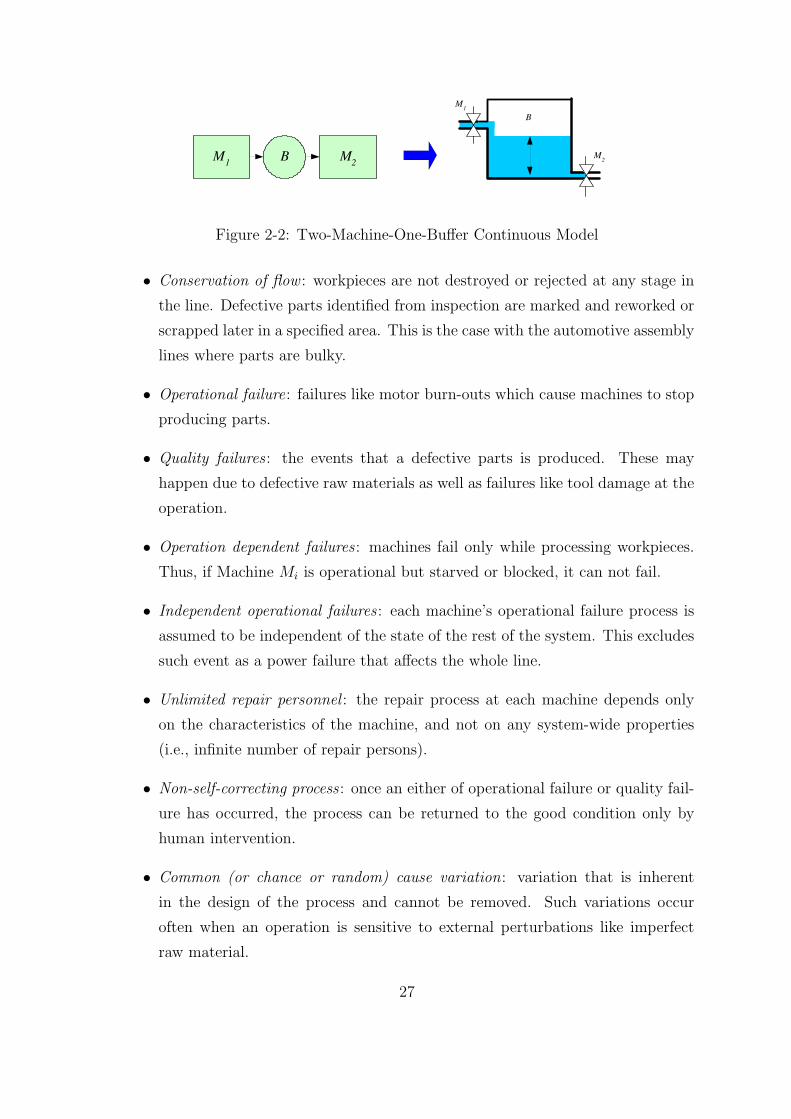
M 1
B M 2
M 2
M 1
B
Figure 2-2: Two-Machine-One-Buffer Continuous Model
• Conservation of flow : workpieces are not destroyed or rejected at any stage in
the line. Defective parts identified from inspection are marked and reworked or
scrapped later in a specified area. This is the case with the automotive assembly
lines where parts are bulky.
• Operational failure: failures like motor burn-outs which cause machines to stop
producing parts.
• Quality failures : the events that a defective parts is produced. These may
happen due to defective raw materials as well as failures like tool damage at the
operation.
• Operation dependent failures : machines fail only while processing workpieces.
Thus, if Machine Mi is operational but starved or blocked, it can not fail.
• Independent operational failures : each machine’s operational failure process is
assumed to be independent of the state of the rest of the system. This excludes
such event as a power failure that affects the whole line.
• Unlimited repair personnel : the repair process at each machine depends only
on the characteristics of the machine, and not on any system-wide properties
(i.e., infinite number of repair persons).
• Non-self-correcting process : once an either of operational failure or quality fail-
ure has occurred, the process can be returned to the good condition only by
human intervention.
• Common (or chance or random) cause variation: variation that is inherent
in the design of the process and cannot be removed. Such variations occur
often when an operation is sensitive to external perturbations like imperfect
raw material.
27

• Assignable (or special or random) cause variation: variation due to a specific,
identifiable cause which changes the process mean or variance.
• Bernoulli quality failures : quality failures due to common cause variations.
Since no permanent changes have occurred in the machine, the occurrence of a
bad part implies nothing about the quality of future parts.
• Persistent quality failures : quality failures due to assignable cause variations.
This kind of quality failures only happen after a change occurs in the machine
or raw material. In that case, once a bad part is produced, all subsequent parts
will be bad until the machine is repaired.
• Multiple-Yield failures : quality failures that occur independently but at different
rates, depending on what state the machine is in. For example, the machine may
produce defective parts with a certain small probability p when it is in good
working order; when it is in need of adjustment, however, it might produce
defective parts with a higher probability q > p.
• Statistical correlation among different quality failures : specific failures are as-
sociated with specific features of a part. Distinct failures may or may not be
correlated with each other depending on the relationship between features, as
well as the sequence in which features are processed by machines:
– Bias (mean-shift) correlation. when a single machine performs several
tasks, or several tools are mounted on a single head, it is possible that a
single misalignment could result in a consistent shift across several different
features.
– Variance correlation. when a single machine performs several tasks, or
several tools are mounted on a single head, it is possible that a single source
of imprecision (e.g. a loose arm) could result in several different features
being out of specification, though not necessarily in the same direction.
– Cumulative effects. in a sequence of operations, it is possible that an
upstream failure results in the malfunctioning of downstream operations as
well, or that a downstream failure results in the corruption of the product of
upstream operations. Thus, multiple failures may occur due to a single root
cause even when operations are performed by physically distinct machines.
28

• Full blockage: machine Mi is fully blocked at time t if one of downstream machine
is down and all buffers between this machine and machine Mi are full.
• Full starvation: machine Mi is fully starved at time t if one of the upstream
machines is down and all buffers between this machine and machine Mi are
empty.
• Partial blockage: machine Mi is partially blocked at time t if one of downstream
machine (Mj) is working slower than Mi (i.e. µj < µi) and all buffers between
Mj and Mi are full. In this case, failure probability rates and inspection rates
need to be reduced. (e.g. pbi = pi
µj
µi, gb
i = giµj
µi, and f b
i = fiµj
µi). Partial blockage
takes place only with continuous models.
• Partial starvation: machine Mi is partially starved at time t if one of upstream
machine (Mj) is working slower than Mi (i.e. µj < µi) and all buffers between
Mj and Mi are empty. In this case, failure probability rates and inspection
rates need to be reduced (e.g. pbi = pi
µj
µi, gb
i = giµj
µi, and f b
i = fiµj
µi). Partial
starvation takes place only with continuous models.
• Operation dependent inspection: inspection is carried out only while a machine
is processing workpieces. Thus, if Machine Mi is operational but starved or
blocked, inspection is not performed.
• Reliability of inspection: there are two kinds of errors in inspection.
– Type I error : error that a good item is classified as defective.
– Type II error : error that a defective item is classified as good.
2.1.2 Modeling assumptions
In this thesis we assume:
• Stationary, saturated, and open systems.
• Continuous models which have deterministic cycle times and full/partial block-
age/starvation.
• Buffer transit time is zero.
29

• Material flow is conserved: defective parts are reworked or scrapped later in a
specified area. No workpieces are destroyed in the line.
• Each machine can have operational failures and quality failures and these fail-
ures are operation dependent.
• All the failures and repairs are uncorrelated.
• Nondestructive and operation dependent inspection which has Type II errors
only.
• Only reactive actions on the failures excluding any of learning effect to people.
2.2 Single machine model
There are many possible ways to characterize the states of a machine for the purpose
of simultaneously studying quality and quantity issues. Here, we model a machine
as a discrete state, continuous time Markov process. Material is assumed continuous,
and µi is the speed at which Machine i processes material while it is operating and
not constrained by the other machine or the buffer. It is a constant, in that µi does
not depend on the repair state of the other machine or the buffer level.
Figure 2-3 shows the proposed state transitions of a single machine with persistent-
type quality failures. In the model, the machine has three states.
• State 1: The machine is operating and producing good parts.
• State -1: The machine is operating and producing bad parts, but the operator
does not know this yet.
• State 0: The machine is not operating.
The machine therefore has two different failure modes (i.e. transition to failure
states from state 1):
• Operational failure: transition from state 1 to state 0. The machine stops
producing parts due to failures like motor burnout.
• Quality failure: transition from state 1 to state -1. The machine stops producing
good parts (and starts producing bad parts) due to a failure like sudden tool
damage.
30

r
p
g f
State 1 State -1 State 0
Figure 2-3: States of a Machine
When a machine is in state 1, it can fail due to a non-quality-related event. It goes
to state 0 with probability rate p. After that an operator fixes it, and the machine
goes back to state 1 with probability rate r. Sometimes, due to an assignable cause,
the machine begins to produce bad parts, so there is a transition from state 1 to state
-1 with a probability rate of g. Here g is the reciprocal of the Mean Time To Quality
Failure (MTQF). A more stable operation leads to a larger MTQF and a smaller g.
The machine, when it is in state -1, can be stopped for two reasons: it may
experience the same kind of operational failure as it does when it is in state 1; or
the operator may stop it for repair when he learns that it is producing bad parts.
The transition from state -1 to state 0 occurs at probability rate f = p + h where h
is the reciprocal of the Mean Time To Detect (MTTD). A more reliable inspection
leads to a shorter MTTD and a larger f . (The detection can take place elsewhere,
for example at a remote inspection station.) Note that this implies that f > p. All
the indicated transition times are assumed to follow exponential distributions.
The machine state definition illustrated in Figure 2-3 is a simplification of a more
generalized machine state definition shown in Figure 2-4. More complex machine state
definition leads to substantially more complicated internal transition equations and
boundary conditions discussed in Chapter 3. Therefore, for simplicity, we assume:
• A machine in a bad condition (i.e., state -1) can be returned to the good condi-
tion (i.e., state 1) only through repair (i.e., state 0). Therefore, a machine does
not have direct state transition from state -1 to state 1 (i.e., q = 0).
• When a machine is under repair (i.e., state 0, state 0’, and state 0”), an op-
erator can not tell whether the machine is down due to a quality failure or an
31
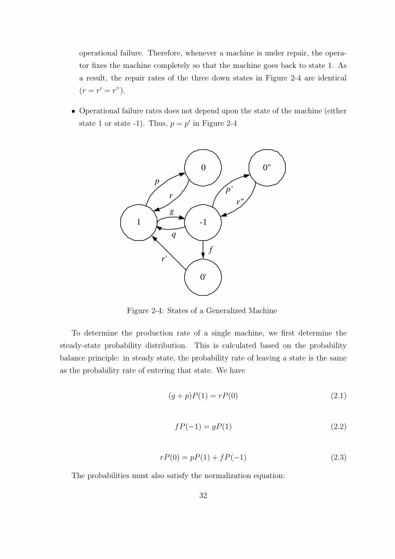
operational failure. Therefore, whenever a machine is under repair, the opera-
tor fixes the machine completely so that the machine goes back to state 1. As
a result, the repair rates of the three down states in Figure 2-4 are identical
(r = r′ = r”).
• Operational failure rates does not depend upon the state of the machine (either
state 1 or state -1). Thus, p = p′ in Figure 2-4
1
r'
p
g
f�
-1
0'
0 0"
r p'
r"
q
Figure 2-4: States of a Generalized Machine
To determine the production rate of a single machine, we first determine the
steady-state probability distribution. This is calculated based on the probability
balance principle: in steady state, the probability rate of leaving a state is the same
as the probability rate of entering that state. We have
(g + p)P (1) = rP (0) (2.1)
fP (−1) = gP (1) (2.2)
rP (0) = pP (1) + fP (−1) (2.3)
The probabilities must also satisfy the normalization equation:
32

P (0) + P (1) + P (−1) = 1 (2.4)
The solution of (2.1)–(2.4) is
P (1) =1
1 + (p + g)/r + g/f(2.5)
P (0) =(p + g)/r
1 + (p + g)/r + g/f(2.6)
P (−1) =g/f
1 + (p + g)/r + g/f(2.7)
The total production rate, including good and bad parts, is
PT = µ(P (1) + P (−1)) = µ1 + g/f
1 + (p + g)/r + g/f(2.8)
The effective production rate, the production rate of good parts only, is
PE = µP (1) = µ1
1 + (p + g)/r + g/f(2.9)
The yield is
PE
PE + PT
=P (1)
P (1) + P (−1)=
f
f + g(2.10)
2.3 Simulation Model
Discrete event simulation models are needed for the validation of the analytic models
developed from the research. A new discrete-event-simulation based on C++ (Qsim)
has been developed and tested to ensure accuracy.
For all the numerical experiments, we used a transient period of 10,000 time
units followed by 1,000,000 time units of data collection period. This ensures that
statistically significant number of events are generated since the typical value of the
mean time to operational failures or quality failures is around 100 time units.
33
2.4 Special two-machine-one-buffer (2M1B) model
2.4.1 Infinite buffer case
An infinite buffer case is a special 2M1B line in which the size of the Buffer (B) is
infinite. This is an extreme case in which the first machine (M1) never suffers from
blockage. To derive expressions for the total production rate and effective production
rate, we observe that when there is infinite buffer capacity between two machines
(M1, M2), the total production rate of the 2M1B system is a minimum of the total
production rates of M1 and M2. The total production rate of machine i is given by
(2.8), so the total production rate of the 2M1B system is
P∞T = min
[µ1(1 + g1/f1)
1 + (p1 + g1)/r1 + g1/f1
,µ2(1 + g2/f2)
1 + (p2 + g2)/r2 + g2/f2
](2.11)
The probability that machine Mi does not add non-conformities is
Yi =Pi(1)
Pi(1) + Pi(−1)=
fi
fi + gi
(2.12)
Since there is no scrap and rework in the system, the system yield is
f1f2
(f1 + g1)(f2 + g2)(2.13)
As a result, the effective production rate is
P∞E =
f1f2
(f1 + g1)(f2 + g2)P∞
T (2.14)
The effective production rate evaluated from (2.14) has been compared with a
discrete-event, discrete-part simulation. The continuous model is a good approxi-
mation since Table 2.1 shows good agreement. The parameters for theses cases are
shown in Appendix A.
2.4.2 Zero buffer case
The zero buffer case is one in which there is no buffer space between the machines.
This is the other extreme case where blockage and starvation take place most fre-
quently.
34

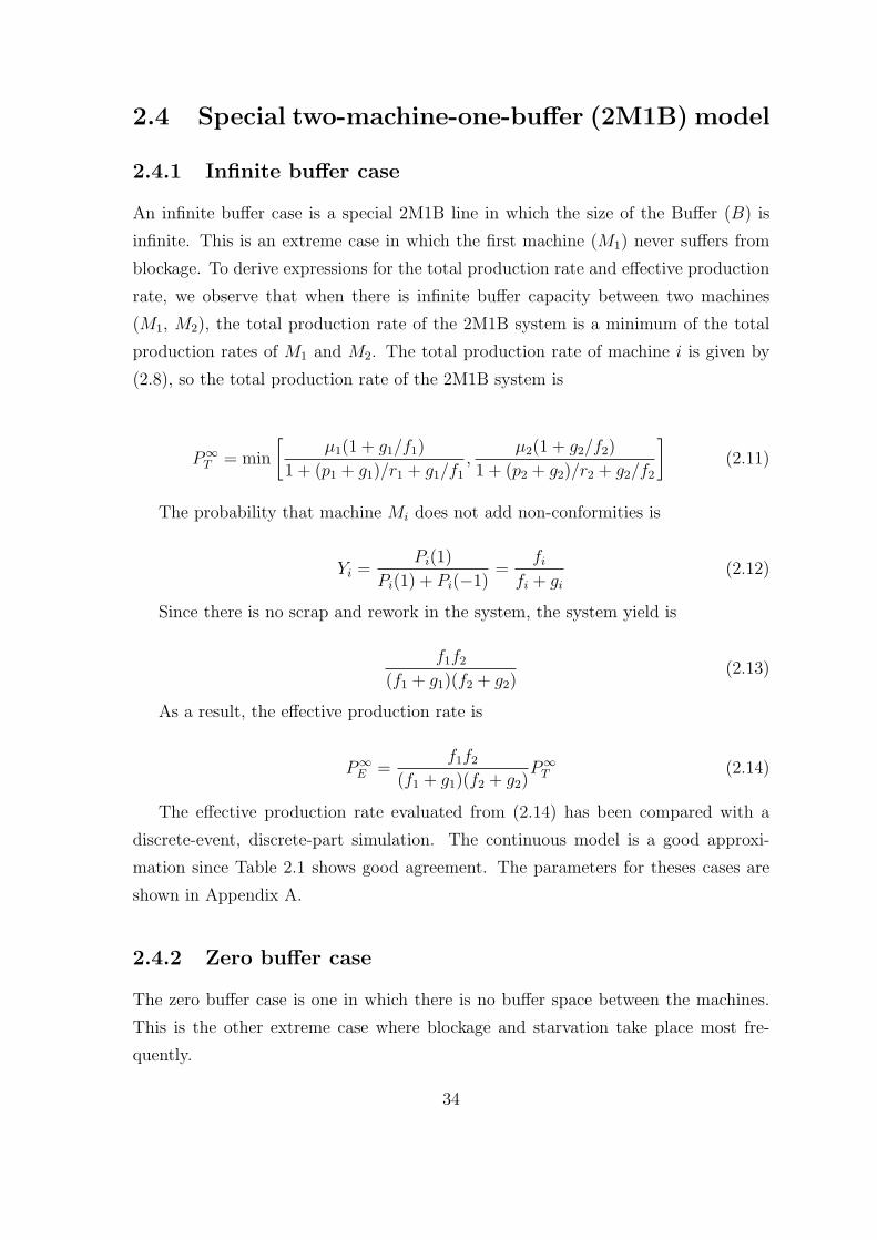
Case # P∞E (Analytic) P∞
E (Simulation) %Difference1 0.762 0.761 0.172 0.708 0.708 0.003 0.657 0.657 -0.004 0.577 0.580 -0.505 0.527 0.530 -0.426 0.745 0.745 0.017 0.762 0.760 0.308 1.524 1.522 0.149 0.762 0.762 0.0010 1.524 1.526 -0.13
Table 2.1: Infinite Buffer Case
In the zero-buffer case in which machines have different operation times, whenever
one of the machines stops, the other one is also stopped. In addition, when both of
them are working, the production rate is min[µ1, µ2]. To calculate the production
rates, consider a long time interval of length T during which M1 fails m1 times and
M2 fails m2 times. If we assume that average time to repair the M1 is 1/r1 and
average time to repair M2 is 1/r2, then the total system down time will be close to
D = m1
r1+ m2
r2. Consequently, total up time will be approximately
U = T −D = T − (m1
r1
+m2
r2
) (2.15)
Since we assume operation-dependent failures, the rates of failure are reduced for
the faster machine. Therefore,
pbi = pi
min(µ1,µ2)µi
, gbi = gi
min(µ1,µ2)µi
and f bi = gi
min(µ1,µ2)µi
The reduction of pi is explained in detail in [Gershwin, 1994]. The reductions of
gi and fi are done for the same reasons.
Table 2.2 lists the possible working states α1 and α2 of M1 and M2. The third
column is the probability of finding the system in the indicated state. The fourth and
fifth columns indicate the expected number of transitions to down states during the
time interval from each of the states in column 1.
From Table (2.2), the expectations of m1 and m2 are
Em1 =1∑
α1=−1
1∑α2=−1
Em1(α1, α2) =Ufb
1 (pb1+gb
1)
fb1+gb
1
Em2 =1∑
α1=−1
1∑α2=−1
Em2(α1, α2) =Ufb
2 (pb2+gb
2)
fb2+gb
2
(2.16)
35
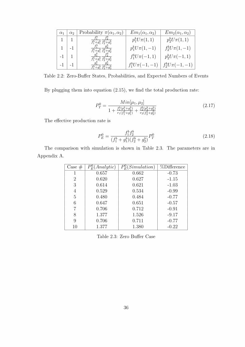
α1 α2 Probability π(α1, α2) Em1(α1, α2) Em2(α1, α2)
1 1fb1
fb1+gb
1
fb2
fb2+gb
2pb
1Uπ(1, 1) pb2Uπ(1, 1)
1 -1fb1
fb1+gb
1
gb2
fb2+gb
2pb
1Uπ(1,−1) f b2Uπ(1,−1)
-1 1gb1
fb1+gb
1
fb2
fb2+gb
2f b
1Uπ(−1, 1) pb2Uπ(−1, 1)
-1 -1gb1
fb1+gb
1
gb2
fb2+gb
2f b
1Uπ(−1,−1) f b2Uπ(−1,−1)
Table 2.2: Zero-Buffer States, Probabilities, and Expected Numbers of Events
By plugging them into equation (2.15), we find the total production rate:
P 0T =
Min[µ1, µ2]
1 +fb1 (pb
1+gb1)
r1(fb1+gb
1)+
fb2 (pb
2+gb2)
r2(fb2+gb
2)
(2.17)
The effective production rate is
P 0E =
f b1f
b2
(f b1 + gb
1)(fb2 + gb
2)P 0
T (2.18)
The comparison with simulation is shown in Table 2.3. The parameters are in
Appendix A.
Case # P 0E(Analytic) P 0
E(Simulation) %Difference1 0.657 0.662 -0.732 0.620 0.627 -1.153 0.614 0.621 -1.034 0.529 0.534 -0.995 0.480 0.484 -0.776 0.647 0.651 -0.577 0.706 0.712 -0.918 1.377 1.526 -9.179 0.706 0.711 -0.7710 1.377 1.380 -0.22
Table 2.3: Zero Buffer Case
36

Chapter 3
Two-Machine-One-Finite-Buffer
(2M1B) Line
In this chapter, we present modeling, solution techniques, and validation of the two-
machine-one-finite-buffer case. The two-machine line is the simplest non-trivial case
of a transfer line. It is used in decomposition approximations of longer lines. (See
Chapter 5.)
3.1 Modeling
3.1.1 State definition
M 1
B 1
M 2
Figure 3-1: Two-machine-one-buffer line
The state of the 2M1B line illustrated in Figure 3-1 is (x, α1, α2) where:
• x: the total amount of material in buffer B. 0 ≤ x ≤ N .
• α1: the state of M1 (α1 = −1, 0, or, 1).
• α2: the state of M2 (α2 = −1, 0, or, 1).
37

The parameters of machine Mi are µi, ri, pi, fi, gi as explained in section 2.2, and
the buffer size is N . The probabilistic behavior of the 2M1B is described by proba-
bility density functions (e.g., f(x, 1, 1)) when buffer B is neither empty nor full, and
by probability masses (e.g., P (0, 1, 1)) when the buffer is either empty or full. If we
find all the probability density functions and the probability masses, we can calculate
the performance measures of the 2M1B line, since these are expressed in terms of
the probability density functions and the probability masses. The probability density
functions and probability masses are to be found by solving the internal transition
equations and the boundary transition equations presented below.
3.1.2 Internal Transition Equations
In this section, we present equations describing behavior of the 2M1B system when
buffer B is neither full nor empty. When buffer B is neither empty nor full, its level
can rise or fall depending on the states of adjacent machines. Since it can change
only a small amount during a short time interval, it is reasonable to use a continuous
probability density f(x, α1, α2) and differential equations to describe its behavior.
The probability of finding both machines at state 1 with a storage level between x
and x + δx at time t + δt is given by f(x, 1, 1, t + δt)δx, where
f(x, 1, 1, t + δt) = {1− (p1 + g1 + p2 + g2)δt}f(x + (µ2 − µ1)δt, 1, 1)
+r2δtf(x− µ1δt, 1, 0) + r1δtf(x + µ2δt, 0, 1) + o(δt)(3.1)
Except for the factor of δx, the first term is the probability of transition from
between (x + (µ2 − µ1)δt, 1, 1) and (x + (µ2 − µ1)δt + δx, 1, 1) at time t to between
(x, 1, 1) and (x + δx, 1, 1) at time t + δt. This is because
• The probability of neither machine failing between t and t + δt is
{1− (p1 + g1)δt}{1− (p2 + g2)δt} ' {1− (p1 + g1 + p2 + g2)δt} (3.2)
• If there are no failures between t and t + δt and the buffer level is between x
and x + δx at time t + δt, then it could only have been between x + (µ2− µ1)δt
and x + (µ2 − µ1)δt + δx at time t.
38
The other terms, which represent the probabilities of transition from (1) machine
states (1,0) with buffer level between x−µ1δt and x−µ1δt+δx and (2) machine states
(0,1) with buffer level between x + µ2δt and (x + µ2δt + δx can be found similarly.
No other transitions are possible. After linearizing, and letting δt → 0, this equation
becomes
∂f(x, 1, 1)
∂t= (µ2−µ1)
∂f(x, 1, 1)
∂x−(p1+g1+p2+g2)f(x, 1, 1)+r2f(x, 1, 0)+r1f(x, 0, 1).
(3.3)
In steady state ∂f∂t
= 0. Then, we have
(µ2−µ1)df(x, 1, 1)
dx− (p1 +g1 +p2 +g2)f(x, 1, 1)+r2f(x, 1, 0)+r1f(x, 0, 1) = 0 (3.4)
In the same way, the eight other internal transition equations for the probability
density function are
p2f(x, 1, 1)− µ1df(x, 1, 0)
dx− (p1 + g1 + r2)f(x, 1, 0) + f2f(x, 1,−1) + r1f(x, 0, 0) = 0
(3.5)
g2f(x, 1, 1)+(µ2−µ1)df(x, 1,−1)
dx−(p1 +g+f2)f(x, 1,−1)+r1f(x, 0,−1) = 0 (3.6)
p1f(x, 1, 1) + µ2df(x, 0, 1)
dx− (r1 + p2 + g2)f(x, 0, 1) + r2f(x, 0, 0) + f1f(x,−1, 1) = 0
(3.7)
p1f(x, 1, 0)+p2f(x, 0, 1)− (r1 +r2)f(x, 0, 0)+f2f(x, 0,−1)+f1f(x,−1, 0) = 0 (3.8)
p1f(x, 1,−1)+g2f(x, 0, 1)− (r1 +f2)f(x, 0,−1)+µ2df(x, 0,−1)
dx+f1f(x,−1,−1) = 0
(3.9)
39
g1f(x, 1, 1)−(p2+g2+f1)f(x,−1, 1)+(µ2−µ1)df(x,−1, 1)
dx+r2f(x,−1, 0) = 0 (3.10)
g1f(x, 1, 0)−µ1df(x,−1, 0)
dx− (r2 +f1)f(x,−1, 0)+p2f(x,−1, 1)+f2f(x,−1,−1) = 0
(3.11)
g1f(x, 1,−1) + g2f(x,−1, 1) + (µ2 − µ1)df(x,−1,−1)
dx− (f1 + f2)f(x,−1,−1) = 0.
(3.12)
3.1.3 Boundary transition equations
While the internal behavior of the system can be described by probability density
functions, there is a nonzero probability of finding the system in certain boundary
states. For example, if µ1 < µ2 and both machines are in state 1, the level of storage
tends to decrease. If both machines remain operational for enough time, the storage
will become empty (x = 0). Once the system reaches state (0, 1, 1), it will remain
there until a machine fails. There are 18 probability masses for boundary states
(P (N, α1, α2) and P (0, α1, α2) where α1 = −1, 0 or 1, and α2 = −1, 0 or 1).
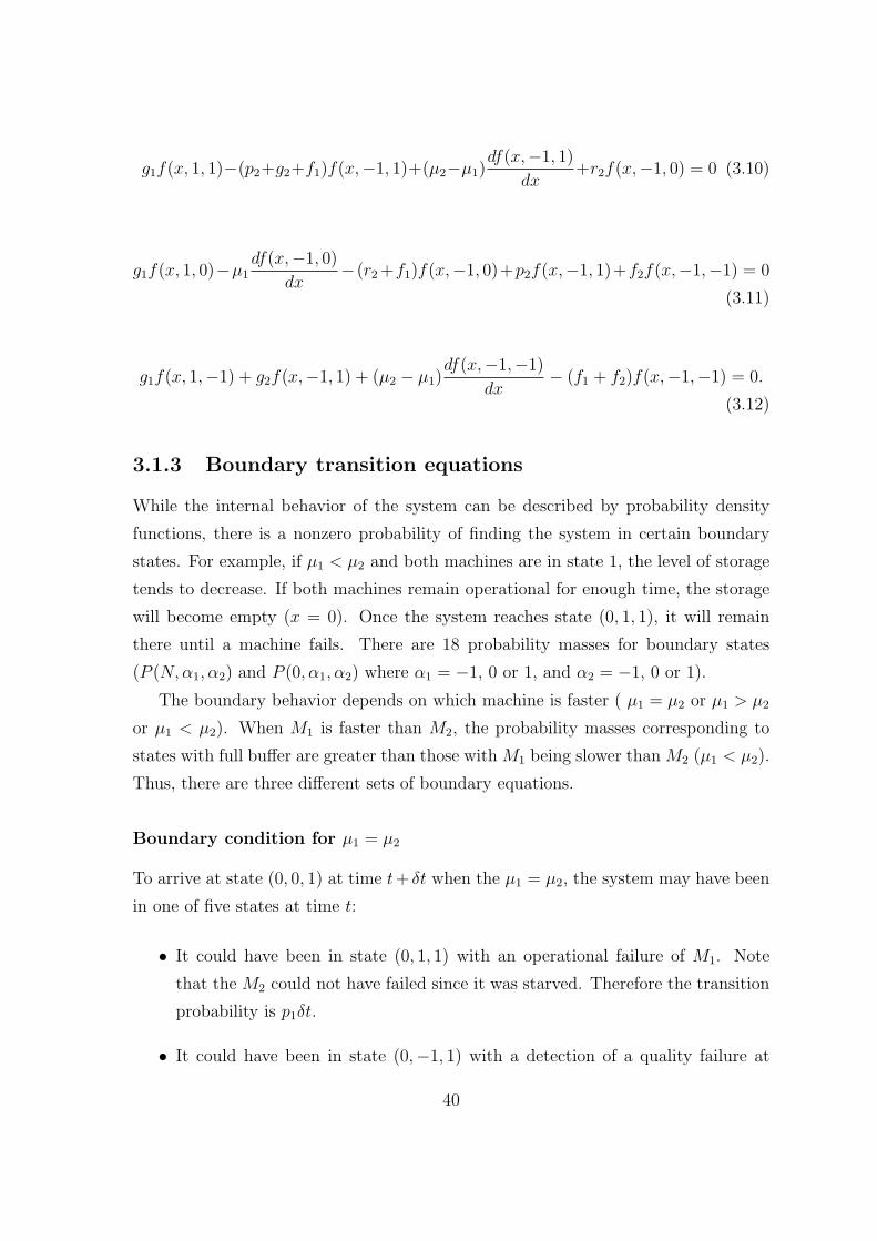
The boundary behavior depends on which machine is faster ( µ1 = µ2 or µ1 > µ2
or µ1 < µ2). When M1 is faster than M2, the probability masses corresponding to
states with full buffer are greater than those with M1 being slower than M2 (µ1 < µ2).
Thus, there are three different sets of boundary equations.
Boundary condition for µ1 = µ2
To arrive at state (0, 0, 1) at time t+ δt when the µ1 = µ2, the system may have been
in one of five states at time t:
• It could have been in state (0, 1, 1) with an operational failure of M1. Note
that the M2 could not have failed since it was starved. Therefore the transition
probability is p1δt.
• It could have been in state (0,−1, 1) with a detection of a quality failure at
40

M1. Again, the M2 could not have failed since it was starved. Therefore the
transition probability is f1δt.
• It could have been in state (0, 0, 1) without repair of M1. The corresponding
transition probability is 1−r1δt since M2 could not have failed due to starvation.
• It could have been in some internal state (x, 0, 1) where 0 ≤ x ≤ µ2δt without
repair of M1 and failure of M2. The corresponding transition probability is
(1− r1δt)(1− (p2 + g2)δt) ' 1− (r1 + p2 + g2)δt.
• It could have been in state (0, 0, 0) with only repair of M2 (not M1). The
corresponding transition probability is (1− r1δt)r2δt ' r2δt.
If the second order terms are ignored,
P (0, 0, 1, t + δt) = p1δtP (0, 1, 1) + f1δtP (0,−1, 1) + (1− r1δt)P (0, 0, 1)
+{1− (r1 + p2 + g2)δt}∫ µ2δt
0f(x, 0, 1)dx + r2δtP (0, 0, 0).
(3.13)
After the usual analysis, (3.13) becomes
∂P (0, 0, 1)
∂t= p1P (0, 1, 1)− r1P (0, 0, 1) + µ2f(0, 0, 1) + f1P (0,−1, 1) + r2P (0, 0, 0).
(3.14)
In steady state, it becomes as equation (3.15)
p1P (0, 1, 1)− r1P (0, 0, 1) + µ2f(0, 0, 1) + f1P (0,−1, 1) + r2P (0, 0, 0) = 0. (3.15)
There are 21 other boundary equations derived similarly for µ1 = µ2:
−(p1 + g1 + p2 + g2)P (0, 1, 1) + r1P (0, 0, 1) = 0. (3.16)
P (0, 1, 0) = 0 (3.17)
g2P (0, 1, 1)− (p1 + g1 + f2)P (0, 1,−1) + r1P (0, 0,−1) = 0 (3.18)
41

−(r1 + r2)P (0, 0, 0) = 0 (3.19)
p1P (0, 1,−1)− r1P (0, 0,−1) + µ2f(0, 0,−1) + f1P (0,−1,−1) = 0 (3.20)
g1P (0, 1, 1)− (f1 + p2 + g2)P (0,−1, 1) = 0 (3.21)
P (0,−1, 0) = 0 (3.22)
g1P (0, 1,−1) + g2P (0,−1, 1)− (f1 + f2)P (0,−1,−1) = 0 (3.23)
−(p1 + g1 + p2 + g2)P (N, 1, 1) + r2P (N, 1, 0) = 0 (3.24)
p2P (N, 1, 1)− r2P (N, 1, 0) + µ1f(N, 1, 0) + f2P (N, 1,−1) + r1P (N, 0, 0) = 0 (3.25)
g2P (N, 1, 1)− (p1 + g1 + f2)P (N, 1,−1) = 0 (3.26)
P (N, 0, 1) = 0 (3.27)
−(r1 + r2)P (N, 0, 0) = 0 (3.28)
P (N, 0,−1) = 0 (3.29)
g1P (N, 1, 1)− (f1 + g2 + p2)P (N,−1, 1) + r2P (N,−1, 0) = 0 (3.30)
−r2P (N,−1, 0) + µ1f(N,−1, 0) + f2P (N,−1,−1) + p2P (N,−1, 1) = 0 (3.31)
42

g1P (N, 1,−1) + g2P (N,−1, 1)− (f1 + f2)P (N,−1,−1) = 0 (3.32)
µ1f(0, 1, 0) = r1P (0, 0, 0) + p2P (0, 1, 1) + f2P (0, 1,−1) (3.33)
µ1f(0,−1, 0) = p2P (0,−1, 1) + f2P (0,−1,−1) (3.34)
µ2f(N, 0, 1) = r2P (N, 0, 0) + p1P (N, 1, 1) + f1P (N,−1, 1) (3.35)
µ2f(N, 0,−1) = p1P (N, 1,−1) + g2P (N, 0, 1) + f1P (N,−1,−1). (3.36)
Boundary condition for µ1 > µ2
When µ1 > µ2, 26 boundary equations can be derived similarly. In this case, there
are 4 more boundary equations than in the µ1 = µ2 cases since it is possible to
reach internal states (x, 1, 1), (x, 1,−1), (x,−1, 1), and (x,−1,−1) (where 0 < x ≤(µ1 − µ2)δt) at time t + δt from the boundary states P (0, α1, α2), (α1 = -1,0,1, and
α2 = -1,0,1) at time t.
µ1f(0, 1, 0) = 0 (3.37)
µ1f(0,−1, 0) = 0 (3.38)
(µ1 − µ2)f(0, 1, 1) = r1P (0, 0, 1) (3.39)
(µ1 − µ2)f(0, 1,−1) = r1P (0, 0,−1) (3.40)
f(0,−1, 1) = 0 (3.41)
f(0,−1,−1) = 0 (3.42)
43

µ2f(N, 0, 1) = pb1P (N, 1, 1) + f b
1P (N,−1, 1) (3.43)
µ2f(N, 0,−1) = pb1P (N, 1,−1) + f b
1P (N,−1,−1) (3.44)
P (0, 1, 1) = 0 (3.45)
P (0, 1, 0) = 0 (3.46)
P (0, 1,−1) = 0 (3.47)
−r1P (0, 0, 1) + µ2f(0, 0, 1) + r2P (0, 0, 0) = 0 (3.48)
P (0, 0, 0) = 0 (3.49)
−r1P (0, 0,−1) + µ2f(0, 0,−1) = 0 (3.50)
P (0,−1, 1) = 0 (3.51)
P (0,−1, 0) = 0 (3.52)
P (0,−1,−1) = 0 (3.53)
−(pb1 + gb
1 + p2 + g2)P (N, 1, 1) + (µ1 − µ2)f(N, 1, 1) + r2P (N, 1, 0) = 0 (3.54)
p2P (N, 1, 1)− r2P (N, 1, 0) + µ1f(N, 1, 0) + f2P (N, 1,−1) + r1P (N, 0, 0) = 0 (3.55)
44
g2P (N, 1, 1)− (pb1 + gb
1 + f2)P (N, 1,−1) + (µ1 − µ2)f(N, 1,−1) = 0 (3.56)
P (N, 0, 1) = 0 (3.57)
P (N, 0, 0) = 0 (3.58)
P (N, 0,−1) = 0 (3.59)
gb1P (N, 1, 1)− (f b
1 + g2 + p2)P (N,−1, 1) + (µ1 − µ2)f(N,−1, 1) + r2P (N,−1, 0) = 0
(3.60)
−r2P (N,−1, 0) + µ1f(N,−1, 0) + f2P (N,−1,−1) + p2P (N,−1, 1) = 0 (3.61)
gb1P (N, 1,−1) + g2P (N,−1, 1)− (f b
1 + f2)P (N,−1,−1) + (µ1 − µ2)f(N,−1,−1) = 0
(3.62)
Boundary condition for µ1 < µ2
Here, the 26 boundary equations for the µ1 < µ2 case are shown.
µ1f(0, 1, 0) = pb2P (0, 1, 1) + f b
2P (0, 1,−1) (3.63)
µ1f(0,−1, 0) = pb2P (0,−1, 1) + f b
2P (0,−1,−1) (3.64)
µ2f(N, 0, 1) = 0 (3.65)
45
µ2f(N, 0,−1) = 0 (3.66)
(µ2 − µ1)f(N, 1, 1) = r2P (N, 1, 0) (3.67)
(µ2 − µ1)f(N,−1, 1) = r2P (N,−1, 0) (3.68)
f(N, 1,−1) = 0 (3.69)
f(N,−1,−1) = 0 (3.70)
−(p1 + g1 + pb2 + gb
2)P (0, 1, 1) + (µ2 − µ1)f(0, 1, 1) + r1P (0, 0, 1) = 0 (3.71)
P (0, 1, 0) = 0 (3.72)
gb2P (0, 1, 1)−(p1+g1+f b
2)P (0, 1,−1)+(µ2−µ1)f(0, 1,−1)+r1P (0, 0,−1) = 0 (3.73)
p1P (0, 1, 1)− r1P (0, 0, 1) + µ2f(0, 0, 1) + f1P (0,−1, 1) + r2P (0, 0, 0) = 0 (3.74)
−(r1 + r2)P (0, 0, 0) = 0 (3.75)
p1P (0, 1,−1)− r1P (0, 0,−1) + µ2f(0, 0,−1) + f1P (0,−1,−1) = 0 (3.76)
g1P (0, 1, 1)− (f1 + pb2 + gb
2)P (0,−1, 1) + (µ2 − µ1)f(0,−1, 1) = 0 (3.77)
46

P (0,−1, 0) = 0 (3.78)
g1P (0, 1,−1) + gb2P (0,−1, 1)− (f1 + f b
2)P (0,−1,−1) + (µ2 − µ1)f(0,−1,−1) = 0
(3.79)
P (N, 1, 1) = 0 (3.80)
−r2P (N, 1, 0) + µ1f(N, 1, 0) + r1P (N, 0, 0) = 0 (3.81)
P (N, 1,−1) = 0 (3.82)
P (N, 0, 1) = 0 (3.83)
P (N, 0, 0) = 0 (3.84)
P (N, 0,−1) = 0 (3.85)
P (N,−1, 1) = 0 (3.86)
−r2P (N,−1, 0) + µ1f(N,−1, 0) + f2P (N,−1,−1) + p2P (N,−1, 1) = 0 (3.87)
P (N,−1,−1) = 0 (3.88)
3.1.4 Normalization
In addition to these, all the probability density functions and probability masses must
satisfy the normalization equation:
47

∑α1=−1,0,1
∑α2=−1,0,1
N∫
0
f(x, α1, α2)dx + P (0, α1, α2) + P (N, α1, α2)
= 1. (3.89)
3.1.5 Performance measures
After finding all probability density functions and probability masses, we can calculate
the average inventory in the buffer from
x =∑
α1=−1,0,1
∑α2=−1,0,1
N∫
0
xf(x, α1, α2)dx + NP (N, α1, α2)
. (3.90)
The total production rate is
PT = P 1T =
∑α2=−1,0,1
µ1[N∫0
{f(x,−1, α2) + f(x, 1, α2)}dx + P (0, 1, α2) + P (0,−1, α2)]
+µ2{P (N, 1,−1) + P (N, 1, 1) + P (N,−1,−1) + P (N,−1, 1}.(3.91)
The rate at which machine M1 produces good parts is
P 1E =
∑α2=−1,0,1
µ1[
N∫
0
f(x, 1, α2)dx+P (0, 1, α2)]+µ2{P (N, 1,−1)+P (N, 1, 1)}. (3.92)
The probability that the first machine produces a non-defective part is then Y1 =
P 1E/PT . The probability that the second machine finishes its operation without adding
a non-conforming feature to a part is Y2 = P 2E/PT where
P 2E =
∑α1=−1,0,1
µ2[
N∫
0
f(x, α1, 1)dx+P (N, α1, 1)]+µ1{P (0,−1, 1)+P (0, 1, 1)}. (3.93)
Therefore, the effective production rate is
PE = Y1Y2PT . (3.94)
48

3.2 Solution technique
3.2.1 Solution to internal transition equations
It is logical to assume an exponential form for the solution to the steady state den-
sity functions since (3.4)–(3.12) are coupled ordinary linear differential equations.
A solution of the form eλxKα11 Kα2
2 worked successfully in the continuous material
two-machine line with perfect quality [Gershwin, 1994]. Therefore, a solution of a
form
f(x, α1, α2) = eλxG1(α1)G2(α2) (3.95)
is assumed here. This form satisfies the transition equations if all of the following
equations are met. Equations (3.4)–(3.12) become, after substituting (3.95) into them,
{(µ2−µ1)λ−(p1+g1+p2+g2)G1(1)G2(1)}+r2G1(1)G2(0)+r1G1(0)G2(1) = 0 (3.96)
−{µ1λ+(p1+g1+r2)}G1(1)G2(0)+p2G1(1)G2(1)+f2G1(1)G2(−1)+r1G1(0)G2(0) = 0
(3.97)
{(µ2−µ1)λ−(p1+g1+f2)}G1(1)G2(−1)+g2G1(1)G2(1)+r1G1(0)G2(−1) = 0 (3.98)
{µ2λ−(r1+p2+g2)}G1(0)G2(1)+p1G1(1)G2(1)+r2G1(0)G2(0)+f1G1(−1)G2(1) = 0
(3.99)
p1G1(1)G2(0)+p2G1(0)G2(1)−(r1+r2)G1(0)G2(0)+f2G1(0)G2(−1)+f1G1(−1)G2(0) = 0
(3.100)
{µ2λ−(r1+f2)}G1(0)G2(−1)+p1G1(1)G2(−1)+g2G1(0)G2(1)+f1G1(−1)G2(−1) = 0
(3.101)
49
{(µ2−µ1)λ−(p2+g2+f1)}G1(−1)G2(1)+g1G1(1)G2(1)+r2G1(−1)G2(0) = 0 (3.102)
−{µ1λ+(r2+f1)}G1(−1)G2(0)+g1G1(1)G2(0)+p2G1(−1)G2(1)+f2G1(−1)G2(−1) = 0
(3.103)
{(µ2−µ1)λ−(f1+f2)}G1(−1)G2(−1)+g1G1(1)G2(−1)+g2G1(−1)G2(1) = 0. (3.104)
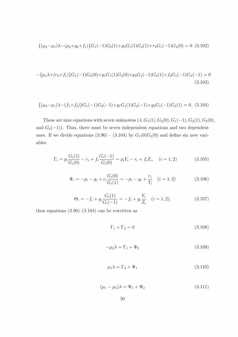
These are nine equations with seven unknowns (λ,G1(1), G2(0), G1(−1), G2(1), G2(0),
and G2(−1)). Thus, there must be seven independent equations and two dependent
ones. If we divide equations (3.96) – (3.104) by G1(0)G2(0) and define six new vari-
ables
Γi = piGi(1)
Gi(0)− ri + fi
Gi(−1)
Gi(0)= piYi − ri + fiZi, (i = 1, 2) (3.105)
Ψi = −pi − gi + riGi(0)
Gi(1)= −pi − gi +
ri
Yi
(i = 1, 2) (3.106)
Θi = −fi + giGi(1)
Gi(−1)= −fi + gi
Yi
Zi
(i = 1, 2). (3.107)
then equations (3.96)–(3.104) can be rewritten as
Γ1 + Γ2 = 0 (3.108)
−µ2λ = Γ1 + Ψ2 (3.109)
µ1λ = Γ2 + Ψ1 (3.110)
(µ1 − µ2)λ = Ψ1 + Ψ2 (3.111)
50

(µ1 − µ2)λ = Θ1 + Θ2 (3.112)
µ1λ = Γ2 + Θ1 (3.113)
−µ2λ = Γ1 + Θ2 (3.114)
(µ1 − µ2)λ = Ψ2 + Θ1 (3.115)
(µ1 − µ2)λ = Ψ1 + Θ2. (3.116)
Equations (3.108) to (3.116) are reduced to seven equation.
Ψ1 = Θ1 (3.117)
Θ1 = µ1λ + Γ1 (3.118)
Ψ2 = Θ2 (3.119)
Θ2 = −µ2λ− Γ1. (3.120)
Γ1 + Γ2 = 0 (3.121)
Combining equations (3.117), (3.106), and (3.107), we have
Ψ1 = µ1λ + Γ1 = −p1 − g1 +r1
Y1
= −f1 + g1Y1
Z1
(3.122)
Ψ2 = −µ2λ− Γ1 = −p2 − g2 +r2
Y2
= −f2 + g2Y2
Z2
. (3.123)
From equation (3.122), we have
Ψ1Y1 = −(p1 + g1)Y1 + r1 (3.124)
51

Ψ1Z1 = −f1Z1 + g1Y1. (3.125)
Together, equations (3.105), (3.124), and (3.125) imply
Ψ1(Y1 + Z1) = −Γ1. (3.126)
Using the same procedure with equations (3.105) and (3.123), we find
Ψ2(Y2 + Z2) = −Γ2 = Γ1. (3.127)
Therefore, we get the new relationship
Ψ1(Y1 + Z1) = −Ψ2(Y2 + Z2). (3.128)
From equations (3.117) and (3.126),
Ψ1 = µ1λ + Γ1 = µ1λ−Ψ1.(Y1 + Z1) (3.129)
Then, we have
Ψ1 =µ1λ
1 + Y1 + Z1
. (3.130)
Using similar procedures,
Ψ2 =−µ2λ
1 + Y2 + Z2
. (3.131)
By plugging equations (3.130) and (3.131) into equation (3.128), we have
µ1(Y1 + Z1)
1 + Y1 + Z1
=µ2(Y2 + Z2)
1 + Y2 + Z2
. (3.132)
Now we try to rewrite the internal transition equations and all the unknowns
used for the equations to two equations and two unknowns by introducing two new
variables. From equations (3.105) and (3.108), we introduce a new variable U :
p1Y1 − r1 + f1Z1 = −(p2Y2 − r2 + f2Z2) = U. (3.133)
52

Another variable V is introduced from equation (3.132):
1
µ1
(1 +1
Y1 + Z1
) =1
µ2
(1 +1
Y2 + Z2
) = V. (3.134)
From equation (3.134), we have
Z1 =1
µ1V − 1− Y1, Z2 =
1
µ2V − 1− Y2. (3.135)
After plugging it into equation (3.133), we have
Y1 =1
p1 − f1
(U + r1 − f1
µ1V − 1), Y2 =
1
p2 − f2
(−U + r2 − f2
µ2V − 1). (3.136)
Also, from equation (3.135),
Y1/Z1=
(µ1V − 1)Y1
1− Y1(µ1V − 1), Y2/Z2
=(µ2V − 1)Y2
1− Y2(µ2V − 1). (3.137)
By using equations (3.136) and (3.137), we can replace Y1, Y2, Y1/Z1, and Y2/Z2
in equations (3.122) and (3.123) and get following two equations:
{(U+r1)(µ1V−1)−f1}2(f1−p1)(µ1V−1)
− {(p1+g1−f1)+r1(µ1V−1)}{(U+r1)(µ1V−1)−f1}(f1−p1)(µ1V−1)
− r1 = 0 (3.138)
{(−U+r2)(µ2V−1)−f2}2(f2−p2)(µ2V−1)
− {(p2+g2−f2)+r2(µ2V−1)}{(−U+r2)(µ2V−1)−f2}(f2−p2)(µ2V−1)
− r2 = 0. (3.139)
Now the 9 transition equations (3.96) - (3.104) and 7 unknowns are simplified into
two equations and two unknowns. By solving these quadratic equations, we can get
U and V . From equations (3.133) and (3.134), we can calculate Y1, Y2, Z1, and Z2.
From these a probability density function (equation (3.95)) can be found per (U, V )
set. The more detailed procedure is presented in sections 3.2.2 and 3.2.3.
3.2.2 Algorithm to solve equations (3.138) and (3.139)
By solving equations (3.138) and (3.139) simultaneously, we can calculate U and
V . An example of these equations is plotted in Figure 3-2. Equation (3.138) is
53

represented as red (lighter) lines and equation (3.139) is shown as blue (darker) lines.
The intersections of the two lines are the solutions of the equations.
Figure 3-2: Plot of Equations (3.138) and (3.139)
These are high order equations for which no general analytical solution exists.
Therefore, a numerical approach is required to find the roots of the equations. But
conventional numerical solvers (e.g., the Newton-Raphson method) can not be used
directly since here are discontinuous ranges in each red (lighter) line and blue (darker)
line as illustrated in Figure 3-2. The coordinates of the end points of the red (lighter)
line are denoted as (Uur , V u
r ) and (U lr, V
lr ). The end points of the blue (darker) lines
are denoted as (Uub , V u
b ) and (U lb, V
lb ). Thus, we need to identify the number of roots of
the equations and regions where roots exist. After that the Newton-Raphson method
is applied to find the exact location of each root.
Characterization of the curves
For the development of an efficient algorithm to find roots of equations (3.138) and
(3.139), we need to characterize their shape. As Figure 3-2 depicts, these curves have
asymptotes and discontinuities. Locating these is the first step in the characterization
of the shape.
Finding asymptotes As shown in Figure 3-2, there are two asymptotes perpendic-
ular to the U axis and and one perpendicular to the V axis for each red (lighter) and
blue (darker) line. We can find asymptotes perpendicular to the U axis as follows.
54
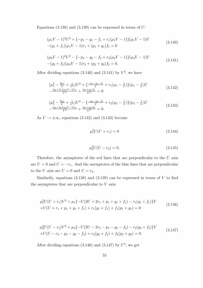
Equations (3.138) and (3.139) can be expressed in terms of U :
(µ1V − 1)2U2 + {−p1 − g1 − f1 + r1(µ1V − 1)}(µ1V − 1)U
−(g1 + f1)(µ1V − 1)r1 + (p1 + g1)f1 = 0(3.140)
(µ2V − 1)2U2 − {−p2 − g2 − f2 + r2(µ2V − 1)}(µ2V − 1)U
−(g2 + f2)(µ2V − 1)r2 + (p2 + g2)f2 = 0.(3.141)
After dividing equations (3.140) and (3.141) by V 2, we have
(µ21 − 2µ1
V+ 1
V 2 )U2 + {−p1−g1−f1
V+ r1(µ1 − 1
V)}(µ1 − 1
V)U
− (g1+f1)(µ1V−1)r1
V 2 + (p1+g1)f1
V 2 = 0(3.142)
(µ22 − 2µ2
V+ 1
V 2 )U2 − {−p2−g2−f2
V+ r2(µ2 − 1
V)}(µ2 − 1
V)U
− (g2+f2)(µ2V−1)r2
V 2 + (p2+g2)f2
V 2 = 0.(3.143)
As V → ±∞, equations (3.142) and (3.143) become
µ21U(U + r1) = 0 (3.144)
µ22U(U − r2) = 0. (3.145)
Therefore, the asymptotes of the red lines that are perpendicular to the U axis
are U = 0 and U = −r1. And the asymptotes of the blue lines that are perpendicular
to the U axis are U = 0 and U = r2.
Similarily, equations (3.138) and (3.139) can be expressed in terms of V to find
the asymptotes that are perpendicular to V axis:
µ21U(U + r1)V
2 + µ1{−U(2U + 2r1 + p1 + g1 + f1)− r1(g1 + f1)}V+U(U + r1 + p1 + g1 + f1) + r1(g1 + f1) + f1(p1 + g1) = 0
(3.146)
µ22U(U − r2)V
2 + µ2{−U(2U − 2r2 − p2 − g2 − f2)− r2(g2 + f2)}V+U(U − r2 − p2 − g2 − f2) + r2(g2 + f2) + f2(p2 + g2) = 0.
(3.147)
After dividing equations (3.146) and (3.147) by U2, we get
55

µ21(1 + r1
U)V 2 + µ1{−(2 + 2r1+p1+g1+f1
U)− r1(g1+f1)
U2 }V+(1 + r1+p1+g1+f1
U) + r1(g1+f1)+f1(p1+g1)
U2 = 0(3.148)
µ22(1− r2
U)V 2 + µ2{−(2 + −2r2−p2−g2−f2
U)− r2(g2+f2)
U2 }V+(1 + −r2−p2−g2−f2
U) + r2(g2+f2)+f2(p2+g2)
U2 = 0(3.149)
As U → ±∞, equations (3.148) and (3.149) become
(µ1V − 1)2 = 0 (3.150)
(µ2V − 1)2 = 0. (3.151)
Therefore, the asymptote of the red lines that is perpendicular to V is V = 1µ1
.
And the asymptote of the blue lines is V = 1µ2
.
Finding discontinuous range The solutions of equation (3.138) are two red lines
whose equations can be re-written as
V = fr(U) = 1µ1
[1 +{(p1+g1+f1)U+(g1+f1)r1}+
√{(p1+g1+f1)U+(g1+f1)r1}2−4U(U+r1)(p1+g1)f1
2U(U+r1)].
(3.152)
V = gr(U) = 1µ1
[1 +{(p1+g1+f1)U+(g1+f1)r1}−
√{(p1+g1+f1)U+(g1+f1)r1}2−4U(U+r1)(p1+g1)f1
2U(U+r1)].
(3.153)
A discontinuous range in the red lines appears where V = fr(U) and V = gr(U)
have complex values. Therefore the U-coordinates of the two end points of the dis-
continuous range in the red lines are the solutions of the equation:
{(p1 + g1 + f1)U + (g1 + f1)r1}2 − 4U(U + r1)(p1 + g1)f1
= (p1 + g1 + f1)2U2 + 2r1{(p1 + g1)(g1 − f1) + f1(g1 + f1)}U + (g1 + f1)
2r21 = 0.
(3.154)
If we set aR = (p1 + g1 + f1)2, bR = 2r1{(p1 + g1)(g1 − f1) + f1(g1 + f1)}, and
cR = (g1 + f1)2r2
1, then,
56

Uur =
−bR −√
b2R − 4aRcR
2aR
, U lr =
−bR +√
b2R − 4aRcR
2aR
. (3.155)
Corresponding V coordinates of the points are given as
V ur =
1
µ1
[1 +(p1 + g1 + f1)U
ur + (g1 + f1)r1
2Uur (Uu
r + r1)]
V lr =
1
µ1
[1 +(p1 + g1 + f1)U
lr + (g1 + f1)r1
2U lr(U
lr + r1)
]. (3.156)
The (Uur , V u
r ) and (U lr, V
lr ) are the coordinates of the end points of the red line as
illustrated in Figure 3-2.
The solutions of equation (3.139) are two blue lines whose equations can be re-
written as:
V = fb(U) = 1µ2
[1 +−{(p2+g2+f2)U−(g2+f2)r2}+
√{(p2+g2+f2)U−(g2+f2)r2}2−4U(U−r2)(p2+g2)f2
2U(U−r2)]
(3.157)
V = gb(U) = 1µ2
[1 +−{(p2+g2+f2)U−(g2+f2)r2}−
√{(p2+g2+f2)U−(g2+f2)r2}2−4U(U−r2)(p2+g2)f2
2U(U−r2)].
(3.158)
Using the same procedure, we can find (Uub , V u
b ) and (U lb, V
lb ), which are the coor-
dinates of the end points of the blue lines as illustrated in Figure 3-2.
Uub =
−bB +√
b2B − 4aBcB
2aB
, U lb =
−bB −√
b2B − 4aBcB
2aB
(3.159)
where aB = (p2 + g2 + f2)2, bB = −2r2{(p2 + g2)(g2 − f2) + f2(g2 + f2)}, and cB =
(g2 + f2)2r2
2
V ub =
1
µ2
[1 +−(p2 + g2 + f2)U
ub + (g2 + f2)r2
2Uub (Uu
b − r2)]
V lr =
1
µ2
[1 +−(p2 + g2 + f2)U
lb + (g2 + f2)r2
2U lb(U
lb − r2)
] (3.160)
57

Region 1
Region 2
Region 3
Region 4
Figure 3-3: Typical shape of the solutions of equations 3.138 and 3.139
Root finding algorithm
Figure 3-3 shows a typical shape of the simplified internal transition equations (i.e.,
equations (3.138) and (3.139)). But the number and the locations of roots vary
depending on machine parameters (i.e. µ1, µ2, r1, r2, p1, p2, g1, g2, f1, and f2) as shown
in Figures 3-4, 3-5, and 3-6.
As illustrated in Figure 3-3, there are four regions in the (U, V ) space in which
roots could possibly exist:
Region 1 There are 3 roots in this region regardless of machine parameters as
depicted in Figure 3-7. The asymptotes of the blue lines are located at U = 0, U = r2,
and the blue lines approach the asymptotes from the left. On the other hand, the
red curves have asymptotes at U = 0, U = −r1 and approach them from the right.
Therefore, one blue curve approaching the asymptote U = r2 meets two of the red
curves. The other blue curve approaching the asymptote U = 0 meets only one red
curve, which approaches the asymptote U = −r1.
Let us define ε as a small number (e.g., order of 10−9) and Ubig as a large number
(e.g., order of 106). We can find these roots in region 1 as follows:
58

−3 −2 −1 0 1 2 3−3
−2
−1
0
1
2
3
U
V
Figure 3-4: Plot of the simplified internal transition equations with µ1 > µ2
−3 −2 −1 0 1 2 3−3
−2
−1
0
1
2
3
U
V
Figure 3-5: Plot of the simplified internal transition equations with µ1 = µ2
−3 −2 −1 0 1 2 3−3
−2
−1
0
1
2
3
U
V
Figure 3-6: Plot of the simplified internal transition equations with µ1 < µ2
59

• One root at the intersection of gb(U) and gr(U) (Root 1 in Figure 3-7) is located
in [−r1 + ε, r2 − ε]. It can be found by solving gb(U) − gr(U) = 0 using the
Newton-Raphson method.
• Another root at intersection of fb(U) and gr(U) (Root 2 in Figure 3-7) is located
in [−r1 +ε,−ε]. It can be found by solving fb(U)−gr(U) = 0 using the Newton-
Raphson method.
• The other root at the intersection of fr(U) and gb(U) is (Root 3 in Figure 3-7)
located in [ε, r2 − ε]. It can be found by solving fr(U) − gb(U) = 0 with the
Newton-Raphson method.
Figure 3-7: Root finding in region 1
Region 3 There are no roots in this area regardless of machine parameters. This
is because the blue lines come from the right hand side and approach the asymptotes
located at U = 0, U = r2. The red lines come from the left hand side and approach
the asymptotes located at U = 0, U = −r1. Thus, the blue lines and red lines can
not intersect with each other.
Region 2 If µ1 ≥ µ2, then there is no root in region 2. Because the blue curves
approach V = 1µ2
from above and the red curves approach V = 1µ1
from below. But
if µ1 < µ2, there are many cases to consider:
60

(1) If f1 > p1 and g1 > 0, there is a gap in the red lines as shown in Figure
(3-8). In this case, the number of roots depends on the location of the gap in the red
lines. In Figure (3-8), (Uur , V u
r ) and (U lr, V
lr ) are the Cartesian coordinates of the end
points of the gap in the red lines.
Here, let us define a new function Hb(U, V ) as
Hb(U, V ) = (V − fb(U))(V − gb(U)). (3.161)
f b (U) g
b (U)
f r (U)
g b (U)
(U r u ,V
r u )
(U r l ,V
r l )
Figure 3-8: Plot of red lines and blue lines with µ1 < µ2 in region 2
The number and the location of roots in region 2 when f1 > p1 and g1 > 0 are as
follows and these roots can be found through the Newton-Raphson method:
• Case 1 : If V lr − fb(U
lr) > 0, there are four roots in the region:
– One from the equation fb(U)− fr(U) = 0 is located in [U lr + ε,−ε].
– Another from the equation fb(U)−gr(U) = 0 is located in [U lr +ε,−r1−ε].
– Another from the equation gb(U)−gr(U) = 0 is located in [U lr +ε,−r1−ε].
– The other from the equation gb(U)− fr(U) = 0 is located in [U lr + ε,−ε].
• Case 2 : If V lr − fb(U
lr) = 0, there are three roots in the region:
– One root is located at (ULr , V L
r ).
– Another from the equation gb(U)−gr(U) = 0 is located in [U lr +ε,−r1−ε].
– The other from the equation gb(U)− fr(U) = 0 is located in [U lr + ε,−ε].
61

Case 1 Case 2
Figure 3-9: Case 1 and Case 2
Case 3 Case 4
Figure 3-10: Case 3 and Case 4
• Case 3 : If V ur − fb(U
ur ) > 0 and Hb(U
lr, V
lr ) < 0, there are two roots in the
region:
– One from the equation gb(U)− gr(U) = 0 is located in [U lr + ε,−r1 − ε].
– The other from the equation gb(U)− fr(U) = 0 is located in [U lr + ε,−ε].
• Case 4 : If V ur − fb(U
ur ) > 0 and V l
r − gb(Ulr) = 0, then one root is located at
(U lr, V
lr ).
Case 5 Case 6
Figure 3-11: Case 5 and Case 6
• Case 5 : If V ur − fb(U
ur ) > 0 and V l
r − gb(Ulr) < 0, then there is no root in the
region.
62
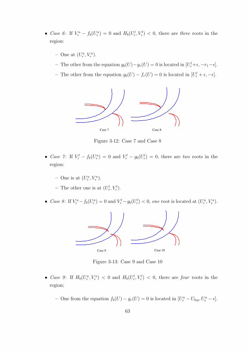
• Case 6 : If V ur − fb(U
ur ) = 0 and Hb(U
lr, V
lr ) < 0, there are three roots in the
region:
– One at (Uur , V u
r ).
– The other from the equation gb(U)−gr(U) = 0 is located in [U lr+ε,−r1−ε].
– The other from the equation gb(U)− fr(U) = 0 is located in [U lr + ε,−ε].
Case 7 Case 8
Figure 3-12: Case 7 and Case 8
• Case 7 : If V lr − fb(U
ur ) = 0 and V l
r − gb(Ulr) = 0, there are two roots in the
region:
– One is at (Uur , V u
r ).
– The other one is at (U lr, V
lr ).
• Case 8 : If V ur −fb(U
ur ) = 0 and V l
r −gb(Ulr) < 0, one root is located at (Uu
r , V ur ).
Case 9 Case 10
Figure 3-13: Case 9 and Case 10
• Case 9 : If Hb(Uur , V u
r ) < 0 and Hb(Ulr, V
lr ) < 0, there are four roots in the
region;
– One from the equation fb(U)− gr(U) = 0 is located in [Uur −Ubig, U
ur − ε].
63

– Another from the equation fb(U)−fr(U) = 0 is located in [Uur −Ubig, U
ur −ε].
– Another from the equation gb(U)−gr(U) = 0 is located in [Uur +ε,−r1−ε].
– The other from the equation gb(U)− fr(U) = 0 is located in [Uur + ε,−ε].
• Case 10 : If Hb(Uur , V u
r ) < 0 and V lr − gb(U
lr) = 0, there are three in the region:
– One is at (Uur , V u
r ).
– Another from the equation fb(U)−gr(U) = 0 is located in [Uur −Ubig, U
ur −ε].
– The other from the equation fb(U)−fr(U) = 0 is located in [Uur −Ubig, U
ur −
ε].
Case 11 Case 12
Figure 3-14: Case 11 and Case 12
• Case 11 : If Hb(Uur , V u
r ) < 0 and V lr − gb(U
lr) < 0, there are two roots in the
region:
– One from the equation fb(U)− gr(U) = 0 is located in [Uur −Ubig, U
ur − ε].
– The other from the equation fb(U)−fr(U) = 0 is located in [Uur −Ubig, U
ur −
ε].
• Case 12 : If V ur − gb(U
ur ) = 0, there are three roots in the region:
– One at (Uur , V u
r ).
– Another from the equation fb(U)−gr(U) = 0 is located in [Uur −Ubig, U
ur −ε].
– The other from the equation fb(U)−fr(U) = 0 is located in [Uur −Ubig, U
ur −
ε].
• Case 13 : If V ur − gb(U
ur ) < 0, there are four roots in the region:
– One from fb(U)− gr(U) = 0 is located in [Uur − Ubig, U
ur − ε].
64

– Another from the equation fb(U)−fr(U) = 0 is located in [Uur −Ubig, U
ur −ε].
– Another from the equation gb(U)−fr(U) = 0 is located in [Uur −Ubig, U
ur −ε].
– The other from the equation gb(U)−gr(U) = 0 is located in [Uur −Ubig, U
ur −
ε].
Case 13 Case 14
Figure 3-15: Case 13 and Case 14
(2) If f1 = g1 or g1 = 0, then there is no gap thus, the equations have 3 or 4
roots. In this case the two red curves intersect at (Uur , V u
r ) = (U lr, V
lr )
• Case 14 : If Hb(Uur , V u
r ) < 0, there are four roots in the region:
– One from the equation fb(U)− gr(U) = 0 is located in [Uur −Ubig,−r1− ε].
– Another from the equation fb(U)− fr(U) = 0 is located in [Uur −Ubig,−ε].
– Another from the equation gb(U)− fr(U) = 0 is located in [Uur + ε,−ε].
– The other from the equation gb(U)−gr(U) = 0 is located in [Uur +ε,−r1−ε].
• Case 15 : If V ur − gb(U
ur ) = 0, there are three in the region:
– One is at (Uur , V u
r ).
– Another from the equation fr(U) = fb(U) is located in [Uur −Ubig, U
ur − ε].
– The other from the equation gr(U) = fb(U) is located in [Uur −Ubig, U
ur −ε].
• Case 16 : If V ur − fb(U
ur ) = 0, there are three roots in the region:
– One is at (Uur , V u
r ).
– Another from the equation fr(u) = gb(u) is located in [Uur + ε,−ε].
– The other from the equation gr(U) = gb(U) is located in [Uur −Ubig,−r1−ε].
65

Case 15 Case 16
Figure 3-16: Case 15 and Case 16
Region 4 If µ1 ≤ µ2, then there is no root in region 4 because the blue curves
approach V = 1µ2
from below and the red curves approach to V = 1µ1
from above.
But if µ1 > µ2, there are many cases to consider;
(1) If f2 > p2 and g2 > 0, there is a gap in the blue lines as shown in Figure
3-17. In this case, the number of roots depends on the location of the gap in the blue
lines. In Figure 3-17, (Uub , V u
b ) and (U lb, V
lb ) are the Cartesian coordinates of the end
points of the gap in the blue lines.
f b (U)
g b (U)
f r (U) g
b (U)
(U b
u ,V b
u )
(U b
l ,V b
l )
Figure 3-17: Plot of red lines and blue lines with µ1 > µ2 in region 4
Here, let us define a new function Hr(U, V ) as
Hr(U, V ) = (V − fr(U))(V − gr(U)). (3.162)
The number and the location of roots in region 4 are as follows and these roots
can be found using the Newton-Raphson method:
66

Case 1 Case 2
Figure 3-18: Case 1 and Case 2
• Case 1 : If V lb − fr(U
lb) > 0, there are four roots in the region:
– One from the equation fr(U)− fb(U) = 0 is located in [ε, U lb − ε].
– Another from the equation fr(U)− gb(U) = 0 is located in [r2 + ε, U lb − ε].
– Another from the equation fr(U)− fb(U) = 0 is located in [ε, U lb − ε].
– The other from the equation gr(U)−gb(U) = 0 is located in [r2 + ε, U lb− ε].
• Case 2 : If V lb − fr(U
lb) = 0, there three roots in the region:
– One is at (U lb, V
lb ).
– Another from the equation gr(U)− fb(U) = 0 is located in [ε, U lb − ε].
– The other from the equation gr(U)−gb(U) = 0 is located in [r2 + ε, U lb− ε].
Case 3 Case 4
Figure 3-19: Case 3 and Case 4
• Case 3 : If V ub − fr(U
ub ) > 0 and Hr(U
lb, V
lb ) < 0, there are two roots in the
region:
– One from the equation gr(U)− fb(U) = 0 is located in [ε, U lb − ε].
– The other from the equation gr(U)−gb(U) = 0 is located in [r2 + ε, U lb− ε].
67

Case 5 Case 6
Figure 3-20: Case 5 and Case 6
• Case 4 : If Uub − fr(U
ub ) > 0 and V l
b − gr(Ulb) = 0, then one root is located at
(U lb, V
lb ).
• Case 5 : If V ub − fr(U
ub ) > 0 and V l
b − gr(Ulb) < 0, then there is no root in the
region.
• Case 6 : If V ub − fr(U
ub ) = 0 and Hr(U
lb, V
lb ) < 0, there are three roots in the
region:
– One is at (Uub , V u
b ).
– Another from the equation gr(U)− fb(U) = 0 is located in [ε, U lb − ε].
– The other from the equation gr(U)−gb(U) = 0 is located in [r2 + ε, U lb− ε].
Case 7 Case 8
Figure 3-21: Case 7 and Case 8
• Case 7 : If V ub − fr(U
ub ) = 0 and V l
b − gr(Ulb) = 0, then two roots are located in
the region:
– One is at (Uub , V u
b ).
– The other is at (U lb, V
lb ).
• Case 8 : If V ub −fr(U
ub ) = 0 and V l
b −gr(Ulb) < 0, one root is located at (Uu
b , V ub ).
68

Case 9 Case 10
Figure 3-22: Case 9 and Case 10
• Case 9 : If Hr(Uub , V u
b ) < 0 and Hr(Ulb, V
lb ) < 0, there are four roots in the
region:
– One from the equation fr(U)− gb(U) = 0 is located in [Uub + ε, Uu
b + Ubig].
– Another from the equation fr(U)−fb(U) = 0 is located in [Uub +ε, Uu
b +Ubig].
– Another from the equation gr(U)− fb(U) = 0 is located in [ε, U lb − ε].
– The other from the equation gr(U)−gb(U) = 0 is located in [r2 + ε, U lb− ε].
• Case 10 : If Hr(Uub , V u
b ) < 0 and V lb − gr(U
lb) = 0, then there are three roots in
the region:
– One is at (U lb, V
lb ).
– One from the equation fr(U)− gb(U) = 0 is located in [Uub + ε, Uu
b + Ubig].
– Another from the equation fr(U)−fb(U) = 0 is located in [Uub +ε, Uu
b +Ubig].
Case 11 Case 12
Figure 3-23: Case 11 and Case 12
• Case 11 : If Hr(Uub , V u
b ) < 0 and V lb − gr(U
lb) < 0, there are two roots in the
region:
– One from the equation fr(U)− gb(U) = 0 is located in [Uub + ε, Uu
b + Ubig].
69

– Another from the equation fr(U)−fb(U) = 0 is located in [Uub +ε, Uu
b +Ubig].
• Case 12 : If V ub − gr(U
ub ) = 0,three roots are located in the region:
– One is at (Uub , V u
b ).
– Another from the equation fr(U)−gb(U) = 0 is located in [Uub +ε, Uu
b +Ubig].
– The other from the equation fr(U)− fb(U) = 0 is located in [Uub + ε, Uu
b +
Ubig].
• Case 13 : If V ub − gr(U
ub ) < 0, there are four roots in the region:
– One from the equation fr(U)− gb(U) = 0 is located in [Uub + ε, Uu
b + Ubig].
– Another from the equation fr(U)−fb(U) = 0 is located in [Uub +ε, Uu
b +Ubig].
– Another from the equation gr(U)−fb(U) = 0 is located in [Uub +ε, Uu
b +Ubig].
– The other from the equation gr(U)− gb(U) = 0 is located in [Uub + ε, Uu
b +
Ubig].
Case 13 Case 14
Figure 3-24: Case 13 and Case 14
(2) If f2 = g2 or g2 = 0, then there is no gap in the blue lines. Thus, the
equations have either 3 or 4 roots. In this case the two blue curves intersect at
(Uub , V u
b ) = (U lb, V
lb ).
• Case 14 If Hr(Uub , V u
b ) < 0, there are four roots in the region:
– One from the equation fb(U)− gr(U) = 0 is located in [ε, Uub − ε].
– Another from the equation fb(U)−fr(U) = 0 is located in [Uub +ε, Uu
b +Ubig].
– Another from the equation gb(U)−fr(U) = 0 is located in [R2+ε, Uub +Ubig].
– The other from the equation gb(U)−gr(U) = 0 is located in [R2+ε, Uub −ε].
70
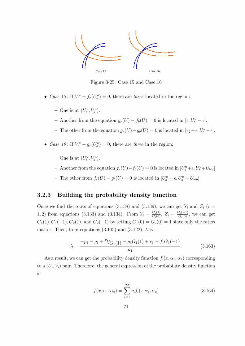
Figure 3-25: Case 15 and Case 16
• Case 15 : If V ub − fr(U
ub ) = 0, there are three located in the region:
– One is at (Uub , V u
b ).
– Another from the equation gr(U)− fb(U) = 0 is located in [ε, Uub − ε].
– The other from the equation gr(U)−gb(U) = 0 is located in [r2 +ε, Uub −ε].
• Case 16 : If V ub − gr(U
ub ) = 0, there are three in the region;
– One is at (Uub , V u
b ).
– Another from the equation fr(U)−fb(U) = 0 is located in [Uub +ε, Uu
b +Ubig]
– The other from fr(U)− gb(U) = 0 is located in [Uub + ε, Uu
b + Ubig]
3.2.3 Building the probability density function
Once we find the roots of equations (3.138) and (3.139), we can get Yi and Zi (i =
1, 2) from equations (3.133) and (3.134). From Yi = Gi(1)Gi(0)
, Zi = Gi(−1)Gi(0)
, we can get
G1(1), G1(−1), G2(1), and G2(−1) by setting G1(0) = G2(0) = 1 since only the ratios
matter. Then, from equations (3.105) and (3.122), λ is
λ =−p1 − g1 + r1/G1(1)− p1G1(1) + r1 − f1G1(−1)
µ1
. (3.163)
As a result, we can get the probability density function fi(x, α1, α2) corresponding
to a (Ui, Vi) pair. Therefore, the general expression of the probability density function
is
f(x, α1, α2) =RN∑i=1
cifi(x,α1, α2) (3.164)
71

where RN is the number of roots of equations (3.138) and (3.139) which is found in
3.2.2.
The remaining unknowns, including coefficients ci i = 1, 2..., RN and probabil-
ity masses at the boundaries, can be calculated by solving the boundary transition
equations and the normalization equation.
3.2.4 Methods to solve boundary conditions
µ1 = µ2 Case
The boundary equations (3.15) – (3.36) are linear equations in which the unknowns
are the probability masses and the coefficients in equation (3.164). Some of the
probability masses are 0 according to the equations, and functions fi(x, α1, α2) are
found by solving the internal transition equations in section 3.2.2. Note that when
µ1 = µ2, the internal transition equations have 3 roots. The boundary equations can
be simplified as follows:
• Drop off the probability masses which are set to 0.
• Temporarily set P (0, 1, 1) = 1.
• Substitute
f(x, α1, α2) = c1f1(x, α1, α2) + c2f2(x, α1, α2) + c3f3(x, α1, α2)
where fi(x, α1, α2) = eλixGi1(α1)G
i2(α2) and Gi
j(1) = Y ij ,Gi
j(0) = 1, and
Gij(−1) = Zi
j (i = 1, 2, 3 and j = 1, 2).
Then, we have an equation AX = B (3.165), which is in matrix form. For example,
the first row of A and B are from equation (3.15). After plugging f(0, 0, 1) = c1Y12 +
c2Y22 + c3Y
32 , into equation (3.15), the equation becomes µ2(c1Y
12 + c2Y
22 + c3Y
32 ) −
r1P (0, 0, 1) + +f1P (0,−1, 1) + p1 = 0. The unknowns (c1, c2, c3, P (0, 0, 1), and
P (0,−1, 1)) are placed at the matrix X, p1 is at B, and the others are at A. After
solving the equation (3.165) using a linear equation solver, all the unknowns are
expressed as multiples of P (0, 1, 1). Then, the value of P (0, 1, 1) can be calculated
from the normalization equation (3.89).
72
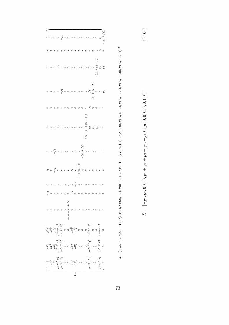
A=
0 B B B B B B B B B B B B B B B B B B B B B B B B B B B B B B B B B B B B @
µY
1 2µ
Y2 2
µY
3 20
−r1
0f1
00
00
00
0
µY
1 1µ
Y2 1
µY
3 1−
f2
00
00
00
00
00
µZ
1 1µ
Z2 1
µZ
3 10
00
−p2
−f2
00
00
00
µe
λ1
NY
1 2µ
eλ2
NY
2 2µ
eλ3
NY
3 20
00
00
−p1
00
−f1
00
µe
λ1
NZ
1 2µ
eλ2
NZ
2 2µ
eλ3
NZ
3 20
00
00
00
−p1
00
−f1
00
00
r1
00
00
00
00
0
00
0−
(p1
+g1
+f2)
0r1
00
00
00
00
µY
1 2µ
Y2 2
µY
3 20
−r1
0f1
00
00
00
0
µZ
1 2µ
Z2 2
µZ
3 2p1
0−
r1
0f1
00
00
00
00
00
00
f1
+p2
+g2
00
00
00
0
00
0g1
00
g2
−(f
1+
f2)
00
00
00
00
00
00
00
−(p
1+
g1
+p2
+g2)
r2
00
00
µe
λ1
NY
1 1µ
eλ2
NY
2 1µ
eλ3
NY
3 10
00
00
p2
−r2
f2
00
0
00
00
00
00
g2
0−
(p1
+g1
+f2)
00
0
00
00
00
00
g1
00
−(f
1+
g2
+p2)
r2
0
µe
λ1
NZ
1 1µ
eλ2
NZ
2 1µ
eλ3
NZ
3 10
00
00
00
0p2
−r2
f2
00
00
00
00
00
g1
g2
0−
(f1
+f2)1 C C C C C C C C C C C C C C C C C C C C C C C C C C C C C C C C C C C C A
X=
[c1,c
2,c
3,P
(0,1
,−1),
P(0
,0,1
),P
(0,0
,−1),
P(0
,−1,1
),P
(0,−
1,−
1),
P(N
,1,1
),P
(N,1
,0),
P(N
,1,−
1),
P(N
,−1,1
),P
(N,−
1,0
),P
(N,−
1,−
1)]
T
B=
[−p 1
,p2,0
,0,0
,p1+
g 1+
p 2+
g 2,−
g 2,0
,g1,0
,0,0
,0,0
,0,0
]T(3
.165
)
73
µ1 > µ2 Case
When µ1 > µ2, the number of roots from the internal transition equations varies from
three to seven depending on machine parameters. The number of roots and the cor-
responding probability density functions are found through the algorithm presented
at 3.2.2.
The boundary equations (3.37) – (3.62) can be simplified:
• Drop off the probability masses which are set to 0.
• Temporarily set P (0, 0, 1) = 1.
• Substitute
f(x, α1, α2) =RN∑i=1
cifi(x, α1, α2)
where RN is the number of roots, fi(x, α1, α2) = eλixGi1(α1)G
i2(α2) and Gi
j(1) =
Y ij ,Gi
j(0) = 1, and Gij(−1) = Zi
j (i = 1, 2, 3 and j = 1, 2).
When there are seven roots from the equations (3.138) and (3.139), we have an
equation AX = B (3.166), which is a matrix form. After solving the equation (3.166)
using a linear equation solver, all the unknowns are expressed as multiples of P (0, 0, 1).
Then, the value of P (0, 0, 1) can be calculated from the normalization equation (3.89).
When there are six roots from the equations (3.138) and (3.139), the number of
unknowns is reduced to 13 from 14. (c7 no longer exists). In this case we can use the
same equation (3.166) and the same procedure after setting c7 = 0. We can do the
same procedure when the internal transition equations have 3, 4, or 5 roots:
• In case of 5 roots, set c7 = 0, c6 = 0.
• In case of 4 roots, set c7 = 0, c6 = 0, and c5 = 0.
• In case of 3 roots, set c7 = 0, c6 = 0, c5 = 0, and , c4 = 0.
Matrix A in equation (3.166) contains elements which can be different by several
orders of magnitude (e.g., eλiNZji Y
ji and Y j
i ). This may cause the reduction of the
apparent rank of matrix A, which will lead to errors. Techniques to prevent this kind
of numerical error are presented in Appendix C.
74

A=
0 B B B B B B B B B B B B B B B B B B B B B B B B B B B B B B B B B B B B B B B B B B B @
Y1 1
Y2 1
Y3 1
Y4 1
Y5 1
Y6 1
Y7 1
00
00
00
0
Z1 1
Z2 1
Z3 1
Z4 1
Z5 1
Z6 1
Z7 1
00
00
00
0
Y1 1Y
1 2Y
2 1Y
2 2Y
3 1Y
3 2Y
4 1Y
4 2Y
5 1Y
5 2Y
6 1Y
6 2Y
7 1Y
7 20
00
00
00
Y1 1Z
1 2Y
2 1Z
2 2Y
3 1Z
3 2Y
4 1Z
4 2Y
5 1Z
5 2Y
6 1Z
6 2Y
7 1Z
7 2−
r1
µD
00
00
00
Z1 1Y
1 2Z
2 1Y
2 2Z
3 1Y
3 2Z
4 1Y
4 2Z
5 1Y
5 2Z
6 1Y
6 2Z
7 1Y
7 20
00
00
00
Z1 1Z
1 2Z
2 1Z
2 2Z
3 1Z
3 2Z
4 1Z
4 2Z
5 1Z
5 2Z
6 1Z
6 2Z
7 1Z
7 20
00
00
00
eλ1
NY
1 2e
λ2
NY
2 2e
λ3
NY
3 2e
λ4
NY
4 2e
λ5
NY
5 2e
λ6
NY
6 2e
λ7
NY
7 20
−p
b 1µ2
00
−f
b 1µ2
00
eλ1
NZ
1 2e
λ2
NZ
2 2e
λ3
NZ
3 2e
λ4
NZ
4 2e
λ5
NZ
5 2e
λ6
NZ
6 2e
λ7
NZ
7 20
00
−p
b 1µ2
00
−f
b 1µ2
Y1 2
Y2 2
Y3 2
Y4 2
Y5 2
Y6 2
Y7 2
00
00
00
0
Z1 2
Z2 2
Z3 2
Z4 2
Z5 2
Z6 2
Z7 2
−r1
µ2
00
00
00
eλ1
NY
1 1Y
1 2e
λ2
NY
2 1Y
2 2e
λ3
NY
3 1Y
3 2e
λ4
NY
4 1Y
4 2e
λ5
NY
5 1Y
5 2e
λ6
NY
1 6Y
6 2e
λ7
NY
7 1Y
7 20
−p
b 1+
gb 1+
p2+
g2
µD
r2
µD
00
00
eλ1
NY
1 1e
λ2
NY
2 1e
λ3
NY
3 1e
λ4
NY
4 1e
λ5
NY
5 1e
λ6
NY
6 1e
λ7
NY
7 10
p2
µ1
−r2
µ1
f2
µ1
00
0
eλ1
NY
1 1Z
1 2e
λ2
NY
2 1Z
2 2e
λ3
NY
3 1Z
3 2e
λ4
NY
4 1Z
4 2e
λ5
NY
5 1Z
5 2e
λ6
NY
6 1Z
6 2e
λ7
NY
7 1Z
7 20
g2
µD
0−
pb 1+
gb 1+
f2
µD
00
0
eλ1
NZ
1 1Y
1 2e
λ2
NZ
2 1Y
2 2e
λ3
NZ
3 1Y
3 2e
λ4
NZ
4 1Y
4 2e
λ5
NZ
5 1Y
5 2e
λ6
NZ
6 1Y
6 2e
λ7
NZ
7 1Y
7 20
gb 1
µD
00
−f
b 1+
g2+
p2
µD
r2
µD
0
eλ1
NZ
1 1e
λ2
NZ
2 1e
λ3
NZ
3 1e
λ4
NZ
4 1e
λ5
NZ
5 1e
λ6
NZ
6 1e
λ7
NZ
7 10
00
0p2
µ1
−r2
µ1
f2
µ1
eλ1
NZ
1 1Z
1 2e
λ2
NZ
2 1Z
2 2e
λ3
NZ
3 1Z
3 2e
λ4
NZ
4 1Z
4 2e
λ5
NZ
5 1Z
5 2e
λ6
NZ
6 1Z
6 2e
λ7
NZ
7 1Z
7 20
00
gb 1
µD
g2
µD
0−
fb 1+
f2
µD
1 C C C C C C C C C C C C C C C C C C C C C C C C C C C C C C C C C C C C C C C C C C C A
X=
[c1,c
2,c
3,c
4,c
5,c
6,c
7,P
(0,0
,−1),
P(N
,1,1
),P
(N,1
,0),
P(N
,1,−
1),
P(N
,−1,1
),P
(N,−
1,0
),P
(N,−
1,−
1)]
T
B=
[0,0
,r 1 µD
,0,0
,0,0
,0,r 1 µ
2
,0,0
,0,0
,0,0
,0]T
(3.1
66)
wher
eµ
D=
µ1−
µ2.
75

µ1 < µ2 Case
When µ1 < µ2, the number of roots from the internal transition equations varies from
three to seven depending on machine parameters. The number of roots and the cor-
responding probability density functions are found through the algorithm presented
at 3.2.2.
The boundary equations (3.63) - (3.88) can be simplified:
• Drop off the probability masses which are set to 0.
• Temporarily set P (0, 1, 1) = 1.
• Substitute
f(x, α1, α2) =RN∑i=1
cifi(x, α1, α2)
where RN is the number of roots, fi(x, α1, α2) = eλixGi1(α1)G
i2(α2) and Gi
j(1) =
Y ij ,Gi
j(0) = 1, and Gij(−1) = Zi
j (i = 1, 2, 3 and j = 1, 2).
When there are seven roots from the equations (3.138) and (3.139), we have a
equation AX = B (3.167), which is a matrix form. After solving the equation (3.167)
using a linear equation solver, all the unknowns are expressed as multiples of P (0, 1, 1).
Then, the value of P (0, 1, 1) can be calculated from the normalization equation (3.89).
When there are six roots from the equations (3.138) and (3.139), the number of
unknowns is reduced to 13 from 14. (c7 no longer exists). In this case we can use the
same equation (3.167) and the same procedure after setting c7 = 0. We can follow
the same procedure when the internal transition equations have 3, 4, or 5 roots:
• In case of 5 roots, set c7 = 0, c6 = 0.
• In case of 4 roots, set c7 = 0, c6 = 0, and c5 = 0.
• In case of 3 roots, set c7 = 0, c6 = 0, c5 = 0, and , c4 = 0.
76

A=
0 B B B B B B B B B B B B B B B B B B B B B B B B B B B B B B B B B B B B B B B B B B B @
Y1 1
Y2 1
Y3 1
Y4 1
Y5 1
Y6 1
Y7 1
−f
b 2µ1
00
00
00
Z1 1
Z2 1
Z3 1
Z4 1
Z5 1
Z6 1
Z7 1
00
0−
pb 2
µ1
−f
b 2µ1
00
eλ1
NY
1 2e
λ2
NY
2 2e
λ3
NY
3 2e
λ4
NY
4 2e
λ5
NY
5 2e
λ6
NY
6 2e
λ7
NY
7 20
00
00
00
eλ1
NZ
1 2e
λ2
NZ
2 2e
λ3
NZ
3 2e
λ4
NZ
4 2e
λ5
NZ
5 2e
λ6
NZ
6 2e
λ7
NZ
7 20
00
00
00
eλ1
NY
1 1Y
1 2e
λ1
NY
2 1Y
2 2e
λ3
NY
3 1Y
3 2e
λ4
NY
4 1Y
4 2e
λ5
NY
5 1Y
5 2e
λ6
NY
6 1Y
6 2e
λ7
NY
7 1Y
7 20
00
00
−r2
µM
0
eλ1
NZ
1 1Y
1 2e
λ2
NZ
2 1Y
2 2e
λ3
NZ
3 1Y
3 2e
λ4
NZ
4 1Y
4 2e
λ5
NZ
5 1Y
5 2e
λ6
NZ
6 1Y
6 2e
λ7
NZ
7 1Y
7 20
00
00
0−
r2
µM
eλ1
NY
1 1Z
1 2e
λ1
NY
2 2Z
2 2e
λ3
NY
3 1Z
3 2e
λ4
NY
4 1Z
4 2e
λ5
NY
5 1Z
5 2e
λ6
NY
6 1Z
6 2e
λ7
NY
7 1Z
7 20
00
00
00
eλ1
NZ
1 1Z
1 2e
λ2
NZ
2 1Z
2 2e
λ3
NZ
3 1Z
3 2e
λ4
NZ
4 1Z
4 2e
λ5
NZ
5 1Z
5 2e
λ6
NZ
6 1Z
6 2e
λ7
NZ
7 1Z
7 20
00
00
00
Y1 1Y
1 2Y
2 1Y
2 2Y
3 1Y
3 2Y
4 1Y
4 2Y
5 1Y
5 2Y
6 1Y
6 2Y
7 1Y
7 20
r1
µM
00
00
0
Y1 1Z
1 2Y
2 1Z
2 2Y
3 1Z
3 2Y
4 1Z
4 2Y
5 1Z
5 2Y
6 1Z
6 2−
f1+
pb 2+
gb 2
µM
00
0
Y1 2
Y2 2
Y3 2
Y4 2
Y5 2
Y6 2
Y7 2
0−
r1
µ2
0f1
µ2
00
0
Z1 2
Z2 2
Z3 2
Z4 2
Z5 2
Z6 2
Z7 2
p1
µ2
0−
r1
µ2
0f1
µ2
00
Z1 1Y
1 2Z
2 1Y
2 2Z
3 1Y
3 2Z
4 1Y
4 2Z
5 1Y
5 2Z
6 1Y
6 2Z
7 1Y
7 20
00
−f1+
pb 2+
gb 2
µM
00
0
Z1 1Z
1 2Z
2 1Z
2 2Z
3 1Z
3 2Z
4 1Z
4 2Z
5 1Z
5 2Z
6 1Z
6 2Z
7 1Z
7 2g1
µM
00
gb 2
µM
−f1+
fb 2
µM
00
eλ1
NY
1 1e
λ2
NY
2 1e
λ3
NY
3 1e
λ4
NY
4 1e
λ5
NY
5 1e
λ6
NY
6 1e
λ7
NY
7 10
00
00
−r2
µ1
0
eλ1
NZ
1 1e
λ2
NZ
2 1e
λ3
NZ
3 1e
λ4
NZ
4 1e
λ5
NZ
5 1e
λ6
NZ
6 1e
λ7
NZ
7 10
00
00
0−
r2
µ1
1 C C C C C C C C C C C C C C C C C C C C C C C C C C C C C C C C C C C C C C C C C C C A
X=
[c1,c
2,c
3,c
4,c
5,c
6,c
7,P
(0,1
,−1),
P(0
,0,1
),P
(0,0
,−1),
P(0
,−1,1
),P
(0,−
1,−
1),
P(N
,1,0
),P
(N,−
1,0
)]T
B=
[pb 2
µ1
,0,0
,0,0
,0,0
,0,p 1
+g 1
+pb 2
+g
b 2
µM
,−g
b 2
µM
,−p 1 µ
2
,0,−
g 1 µM
,0,0
,0]T
(3.1
67)
wher
eµ
M=
µ2−
µ1.
77
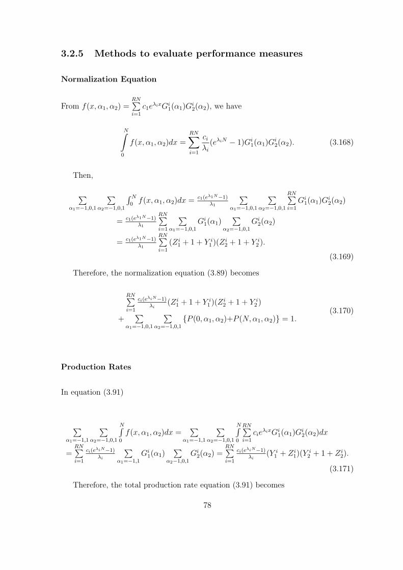
3.2.5 Methods to evaluate performance measures
Normalization Equation
From f(x, α1, α2) =RN∑i=1
c1eλixGi
1(α1)Gi2(α2), we have
N∫
0
f(x, α1, α2)dx =RN∑i=1
ci
λi
(eλiN − 1)Gi1(α1)G
i2(α2). (3.168)
Then,
∑α1=−1,0,1
∑α2=−1,0,1
∫ N
0f(x, α1, α2)dx = c1(eλ1N−1)
λ1
∑α1=−1,0,1
∑α2=−1,0,1
RN∑i=1
Gi1(α1)G
i2(α2)
= c1(eλ1N−1)λ1
RN∑i=1
∑α1=−1,0,1
Gi1(α1)
∑α2=−1,0,1
Gi2(α2)
= c1(eλ1N−1)λ1
RN∑i=1
(Zi1 + 1 + Y i
1 )(Zi2 + 1 + Y i
2 ).
(3.169)
Therefore, the normalization equation (3.89) becomes
RN∑i=1
ci(eλiN−1)λi
(Zi1 + 1 + Y i
1 )(Zi2 + 1 + Y i
2 )
+∑
α1=−1,0,1
∑α2=−1,0,1
{P (0, α1, α2)+P (N,α1, α2)} = 1.(3.170)
Production Rates
In equation (3.91)
∑α1=−1,1
∑α2=−1,0,1
N∫0
f(x, α1, α2)dx =∑
α1=−1,1
∑α2=−1,0,1
N∫0
RN∑i=1
cieλixGi
1(α1)Gi2(α2)dx
=RN∑i=1
ci(eλiN−1)λi
∑α1=−1,1
Gi1(α1)
∑α2−1,0,1
Gi2(α2) =
RN∑i=1
ci(eλiN−1)λi
(Y i1 + Zi
1)(Yi2 + 1 + Zi
2).
(3.171)
Therefore, the total production rate equation (3.91) becomes
78

P 1T = µ1
RN∑i=1
ci(eλiN−1)λi
(Y i1 + Zi
1)(Yi2 + 1 + Zi
2)+µ1
∑α2=−1,0,1
{P (0, 1, α2) + P (0,−1, α2)}
+µ2{P (N,−1,−1) + P (N,−1, 1) + P (N, 1,−1) + P (N, 1, 1)}.(3.172)
Finally the same procedure, P 1E (equation (3.92)) is expressed as
µ1[RN∑i=1
ciYi1 (Y i
2 + 1 + Zi2)
eλiN − 1
λi
+µ1
∑α2=−1,0,1
P (0, 1, α2)+µ2{P (N, 1,−1)+P (N, 1, 1)}
(3.173)
and P 2E (equation (3.93)) becomes
µ2[RN∑i=1
ciYi2 (Y i
1 + 1 + Zi1)
eλiN − 1
λi
+µ2
∑α1=−1,0,1
P (N,α1, 1) + µ1{P (0, 1,−1) + P (0, 1, 1)}
(3.174)
Average Inventory
In equation (3.90),
∑α1=−1,0,1
∑α2=−1,0,1
N∫0
xf(x, α1, α2)dx =∑
α1=−1,0,1
∑α2=−1,0,1
N∫0
[xRN∑i=1
cieλixGi
1(α1)Gi2(α2)]dx
=RN∑i=1
[ci
N∫0
xeλixdx∑
α1=−1,0,1
Gi1(α1)
∑α2=−1,0,1
Gi2(α2)]
=RN∑i=1
[ci(Yi1 + 1 + Zi
1)(Yi2 + 1 + Zi
2)N∫0
xeλixdx].
(3.175)
From integration by parts,∫
f ′g = fg − ∫fg′, we can set f ′ = eλx, g = x. Then, we
have
N∫0
xeλxdx = [xλeλx]N0 −
N∫0
1λeλxdx = N
λeλN − 1
λ2 (eλN − 1) (if λ 6= 0)
= N2/2 (if λ = 0)
(3.176)
Finally, the average inventory equation (equation (3.90)) becomes
79

X =RN∑i=1
[ci(Yi1 + 1 + Zi
1)(Yi2 + 1 + Zi
2)(Nλi
eλiN − eλiN−1λ2
i)]
N∑
α1=−1,0,1
∑α2=−1,0,1
P (N, α1, α2)(3.177)
3.3 Validation
A mathematical model for the two-machine-one-finite-buffer system has been solved.
But as we have indicated, we present discrete parts in this model as a continuous
fluid and time as a continuous variable. On the other hand, in simulation and in
most real systems, both material and time are discrete. We compare analytical and
simulation results in this section. For simulation, transient period of 10,000 time units
and 1,000,000 time units of data collection period are used. For each case, the half
widths of the 95% confidence intervals on the total production rate and the effective
production rates fall below 1% of their mean values. Also, the half widths of the 95%
confidence intervals on the average inventory become less than 3% of the nominal
value of average inventory for all cases.
Figure 3-26: Validation of the total production rate
Figures 3-26, 3-27, and 3-28 illustrate the comparison of the total production rate,
the effective production rate, and the average inventory from the analytic model and
the simulation respectively. By changing machine and buffer parameters, 100 cases
are generated and % errors are plotted in the vertical axis. The parameters for these
cases are given in Appendix A. The % errors in the production rates are calculated
80
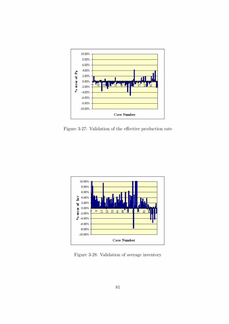
Figure 3-27: Validation of the effective production rate
Figure 3-28: Validation of average inventory
81
from
PT %error =PT (A)− PT (S)
PT (S)× 100(%)
PE %error =PE(A)− PE(S)
PE(S)× 100(%) (3.178)
where PT (A) and PE(A) are the total production rate and the effective production rate
calculated from the analytical model, and PT (S) and PE(S) are the total production
rate and the effective production rate estimated from the simulation. But the % error
in the average inventory is calculated from
Inv %error =Inv(A)− Inv(S)
0.5×N× 100(%) (3.179)
where Inv(A) and Inv(S) are average inventory estimated from the analytical model
and the simulation respectively and N is buffer size. This equation is an unbiased
way to calculate the error in average inventory. If it were calculated in the same way
as the error in the production rates, the error would depend on the relative speeds of
the machines. This is because there will be a lower error when the buffer is mostly
full (i.e., when M1 is faster than M2) and a higher error when the buffer is empty
(i.e., when M1 is slower than M2).
The average absolute value of the % errors in the total production rate, the ef-
fective production rate, and the average inventory are 0.49%, 0.92%, and 3.22% re-
spectively. The estimate of total production rate shows less error than that of the
effective production rate. The observation that the production rates estimates are
better than average buffer levels is consistent with the rest of literature [Dallery and
Gershwin, 1992], [Burman, 1995].
3.4 Quality information feedback
Factory designers and managers know that it is ideal to have inspection after every
operation. However, it is often costly to do this. As a result, factories are usually
designed so that multiple inspections are performed at a small number of stations.
In this case, inspection at downstream operations can detect bad features made by
upstream machines. (We call this quality information feedback.). A simple example
of the quality information feedback in 2M1B systems is when M1 produces defective
82

features but does not have inspection, and M2 has inspection and it can detect bad
features made by M1. In this situation, as we demonstrate below, the yield of a line
is a function of the size of the buffer. When the buffer gets larger, more material
can accumulate between an operation (M1) and the inspection of that operation
(M2). All such material will be defective if a persistent quality failure takes place.
In other words, if the buffer is larger, there tends to be more material in the buffer
and consequently more material is produced before detection occurs. In addition,
it takes longer to have inspections after finishing operations. We can capture this
phenomenon with the adjustment of the transition probability rate of M1 from state
-1 to state 0.
Let us define f q1 as the transition rate of M1 from state -1 to state 0 when there is
quality information feedback and f1 as the transition rate without quality information
feedback. The adjustment can be done in a way that the yield of M1 becomes the
same asKg
1
Kg1+Kb
1where:
• Kb1 : the expected number of bad parts generated by M1 from the time it enters
state -1 until it leaves state -1.
• Kg1 : the expected number of good parts produced by M1 from the moment
when M1 leaves the -1 state to the next time it arrives at state -1.
From equations (2.5), (2.6), and (2.5), the yield of M1 is
P (1)
P (1) + P (−1)=
f q1
f q1 + g1
. (3.180)
Suppose that M1 has been in state 1 for a long time. Then all parts in the buffer
B are non-defective. Suppose that M1 then goes to state -1. Defective parts will then
begin to accumulate in the buffer. Until all the parts in the buffer are defective, the
only way that M1 can go to state 0 is due to its own inspection or its own operational
failures. Therefore, the probability of a transition to 0 before M1 finishes a part is
χ11 =f1
µ1
. (3.181)
Note that f1 ≤ µ1 since the detection of bad feature can not be done before the
completion of making the feature.
Eventually all the parts in the buffer are bad, so that defective parts reach M2.
Then, there is another way that M1 can move to state 0 from state -1: quality
83

information feedback. The probability that inspection at M2 detects a nonconformity
made by M1 is
χ21 =h21
µ2
(3.182)
where 1h21
is the mean time until the inspection at M2 detects a bad part made by
M1 after M2 receives the bad part.
The expected number of bad parts produced by M1 before it is stopped by either
operational failures or quality information feedback is
Kb1 = [χ11 + 2χ11(1− χ11) + 3χ11(1− χ11)
2 + . . . + wχ11(1− χ11)w−1]
+[(w + 1)(1− χ11)wχ21 + (w + 2)(1− χ11)
w+1χ21(1− χ21) + . . .](3.183)
where w is average inventory in the buffer B. This is an approximation since we simply
use the average inventory rather than averaging the expected number of bad parts
produced by M1 depending on different inventory levels wi. After some mathematical
manipulation,
Kb1 =
1− (1− χ11)w
χ11
− w(1− χ11)w +
(1− χ11)wχ21[(w + 1)− w(1− χ11)(1− χ21)]
[1− (1− χ11)(1− χ21)]2
(3.184)
On the other hand, Kg1 is given as
Kg1 =
µ1
p1 + g1
+p1
p1 + g1
µ1
p1 + g1
+ (p1
p1 + g1
)2
(µ1
p1 + g1
) . . . =µ1
g1
(3.185)
By settingfq1
fq1 +g1
=Kg
1
Kg1+Kb
1we have
f q1 =
µ1
1−(1+wχ11)(1−χ11)w
χ11+ (1−χ11)wχ21[1+w(χ21+χ11−χ21χ11)]
[1−(1−χ11)(1−χ21)]2
(3.186)
Since the average inventory is a function of f q1 and f q
1 is dependent on the average
inventory, an iterative method is used to get these values.
Figures 3-29, 3-30, and 3-31 show the comparison of the total production rate,
the effective production rate and the average inventory from the analytic model and
the simulation. By selecting different machines and buffer parameters, 50 cases are
generated, and % errors are plotted in the vertical axes. The parameters for these
84

Figure 3-29: Quality information feedback: total production rate
Figure 3-30: Quality information feedback: effective production rate
Figure 3-31: Quality information feedback: average inventory
85

cases are given in Appendix A. % errors in the effective production rate and average
inventory are calculated using equations (3.178) and (3.179) respectively. The average
absolute value of the % error in PT , PE and x estimates are 0.38%, 0.46%, and
5.64% respectively. Comparisons of average inventory (Figures 3.179 and 3-31) reveal
that the estimation from the analytical model have positive bias. This bias happens
because the minimum buffer size is 1 for the simulation whereas it is 0 for the analytic
model; when 2M1B system with buffer size N is compared, the simulation treats the
system as if it has N−1 effective buffer space, but the analytic model uses N effective
buffer space.
86

Chapter 4
Insights From Numerical
Experimentation
In this chapter, we describe a set of numerical experiments that provide intuitive
insight into the behavior of 2M1B systems with quality and productivity issues. The
parameters of all the cases are presented in Appendix A.
4.1 Beneficial buffer case
In this section, we describe a case in which a larger buffer leads to the higher effective
production rate as well as the more total production rate.
4.1.1 Production rates
Having quality feedback means having more inspections than otherwise. Therefore,
machines tend to stop more frequently. As a result, the total production rate of
the line decreases. However, the effective production rate can increase since added
inspections prevent the making of defective parts. This phenomenon is shown in Fig-
ures 4-1 and 4-2. Note that the total production rate PT without quality information
feedback is consistently higher than PT with quality information feedback regardless
of buffer size, and the opposite is true for the effective production rate PE. In the
beneficial buffer case, it should be noted that both the total production rate and the
effective production rate increase with buffer size, with or without quality information
feedback.
87

0 5 10 15 20 25 30 35 40 45 500.65
0.7
0.75
0.8
Buffer Size
Tot
al P
rodu
ctio
n R
ate
without feedbackwith feedback
Figure 4-1: Beneficial Buffer Case: Total Production Rate
0 5 10 15 20 25 30 35 40 45 500.65
0.7
0.75
0.8
Buffer Size
Effe
ctiv
e P
rodu
ctio
n R
ate
without feedbackwith feedback
Figure 4-2: Beneficial Buffer Case: Effective Production Rate
88

4.1.2 System yield and buffer size
Even though a larger buffer increases both total and effective production rates in this
case, it decreases yield. As explained in Section 3.4, the system yield is a function of
the buffer size if there is quality information feedback. Figure 4-3 depicts system yield
decreasing as buffer size increases when there is quality information feedback. This
relationship happens because when the buffer gets larger, more material accumulates
between an operation and the inspection of that operation. All such material will be
defective when the first machine is at state -1 but the inspection at the first machine
does not find it. This is a case in which a smaller buffer improves quality, which is
widely believed to be generally true. If there is no quality information feedback, then
the system yield is independent of the buffer size (and is substantially less).
0 5 10 15 20 25 30 35 40 45 500.89
0.9
0.91
0.92
0.93
0.94
0.95
0.96
0.97
Buffer Size
Sys
tem
Yie
ld
without feedbackwith feedback
Figure 4-3: Beneficial Buffer Case: System Yield as a Function of Buffer Size
4.2 Harmful buffer case
4.2.1 Production rates
Typically, increasing the buffer size leads to higher effective production rate. This
relationship is illustrated in Figure 4-2. But under certain conditions, the effective
production rate can actually decrease as buffer size increases. This phenomenon can
happen when:
• The first machine produces bad parts frequently: this means g1 is large.
89

• The inspection at the first machine is poor or non-existent and inspection at
the second machine is reliable: this means h1 << h2 or f1 − p1 << f2 − p2.
• There is quality information feedback.
• The isolated production rate of the first machine is higher than that of the
second machine:
µ1(1 + g1/f1)
1 + (p1 + g1)/r1 + g1/f1
>µ2(1 + g2/f2)
1 + (p2 + g2)/r2 + g2/f2
.
Figure 4-4 presents a case in which a buffer size increase leads to a lower effective
production rate. Note that even in this case the total production rate monotonically
increases as buffer size increases (See Figure 4-5).
0 5 10 15 20 25 30 35 40 45 500
0.5
1
1.5
Buffer Size
Effe
ctiv
e P
rodu
ctio
n R
ate
Without feedbackWith feedback
Figure 4-4: Harmful Buffer Case: Effective Production Rate
4.2.2 System Yield
The system yield for this case is shown in Figure 4-6. Note that the yield decreases
dramatically as the buffer size increases. In this case, the decrease of the system yield
is more than the increase of the total production rate so that the effective production
rate monotonically decreases as buffer gets bigger.
90

0 5 10 15 20 25 30 35 40 45 500
0.5
1
1.5
Buffer Size
Tot
al P
rodu
ctio
n R
ate
Without feedbackWith feedback
Figure 4-5: Harmful Buffer Case: Total Production Rate
0 5 10 15 20 25 30 35 40 45 500
0.1
0.2
0.3
0.4
0.5
0.6
0.7
0.8
0.9
1
Buffer Size
Sys
tem
Yie
ld
Without feedbackWith feedback
Figure 4-6: Harmful Buffer Case: System Yield as a Function of Buffer Size
4.3 Optimal buffer case
As demonstrated in Figure 4-7, there are cases in which the effective production
rate increases up to a certain level then decreases as the buffer size (N) increases.
In this situation, we have an optimal buffer level N∗ that maximizes the effective
production rate. When N < N∗, as the buffer size gets bigger, the increase of the
total production rate is more than the decrease of the system yield. Therefore, the
effective production rate, which is a multiplication of the total production rate and
the buffer size, increases. But it decreases as the buffer size gets bigger when N > N∗
91

since the decrease of the system yield excels the increase of the total production rate.
The behaviors of the total production rate and the system yield are shown in Figures
4-8 and 4-9.
0 5 10 15 20 25 30 35 40 45 500.37
0.375
0.38
0.385
0.39
0.395
0.4
Buffer Size
Effe
ctiv
e P
rodu
ctio
n R
ate
Figure 4-7: Optimal Buffer Size Case: Effective Production Rate
0 5 10 15 20 25 30 35 40 45 500.4
0.42
0.44
0.46
0.48
0.5
0.52
0.54
Buffer Size
Tot
al P
rodu
ctio
n R
ate
Figure 4-8: Optimal Buffer Size Case: Total Production Rate
92

0 5 10 15 20 25 30 35 40 45 500.65
0.7
0.75
0.8
0.85
0.9
0.95
1
Buffer Size
Sys
tem
Yie
ld
Figure 4-9: Optimal Buffer Size Case: System Yield
4.4 How to improve quality in a line with
persistent quality failures
Quality can be improved in two major ways. One way is to increase the yield of indi-
vidual operations, and the other is to perform more rigorous inspection. Performing
extensive preventive maintenance on manufacturing equipment and using robust en-
gineering techniques to stabilize operations have been suggested as tools to increase
yield of individual operations. Both approaches increase the mean time to quality
failure (MTQF ) (i.e., decrease g). On the other hand, the inspection policy aims to
detect bad parts as soon as possible and to prevent their flow toward downstream
operations. More rigorous inspection decreases the mean time to detect (MTTD)
(i.e., increases h and therefore increases f). It is reasonable to believe that using only
one kind of method to achieve a target quality level would not give the most cost
efficient quality assurance policy. Figure 4-10 indicates that the impact of individual
operation stabilization on the system yield decreases as the operation becomes more
stable. Figure 4-11 shows that effect of improving inspection (MTTD) on the system
yield decreases as inspection becomes more reliable. Therefore, it is optimal to use a
combination of both methods to improve quality.
93

50 100 150 200 250 300 350 400 4500
0.1
0.2
0.3
0.4
0.5
0.6
0.7
0.8
0.9
1
MTQF
Sys
tem
Yie
ld
Figure 4-10: Quality Improvement Through Increase of MTQF
0 0.1 0.2 0.3 0.4 0.5 0.6 0.7 0.8 0.9 10
0.1
0.2
0.3
0.4
0.5
0.6
0.7
0.8
0.9
1
f = p+h
Sys
tem
Yie
ld
Figure 4-11: Quality Improvement Through Increase of f
94

4.5 How to increase the effective production rate
Improving the stand-alone throughput of each operation and increasing buffer space
are typical ways to increase the production rates of manufacturing systems. If opera-
tions are apt to have quality failures, however, there may be other ways to increase the
effective production rate: increasing the yield of each operation and conducting more
reliable inspections. Stabilizing operations, thus improving the yield of individual
operations, will increase effective throughput of a manufacturing system regardless
of the type of quality failure. On the other hand, reducing the mean time to de-
tect (MTTD) will increase the effective production rate only if the quality failure is
persistent, but it will decrease the effective production rate if the quality failure is
Bernoulli. This phenomenon occurs because the quality of each part is independent
of the others when the quality failure is Bernoulli. Therefore, stopping the line does
not reduce the number of bad parts in the future.
In a situation in which machines produce defective parts frequently and inspection
is poor, increasing inspection reliability is more effective than increasing buffer size
to boost the effective production rate. Figure 4-12 demonstrates this. Also, in other
situations in which machines produce defective parts frequently and inspection is
reliable, increasing machine stability is more effective than increasing buffer size to
enhance effective production rate. Figure 4-13 depicts this phenomenon.
0 5 10 15 20 25 30 35 400.5
0.55
0.6
0.65
0.7
0.75
0.8
Buffer Size
Effe
ctiv
e P
rodu
ctio
n R
ate
MTTD = 20MTTD = 10MTTD = 2
Figure 4-12: Mean Time to Detect and Effective Production Rate
95
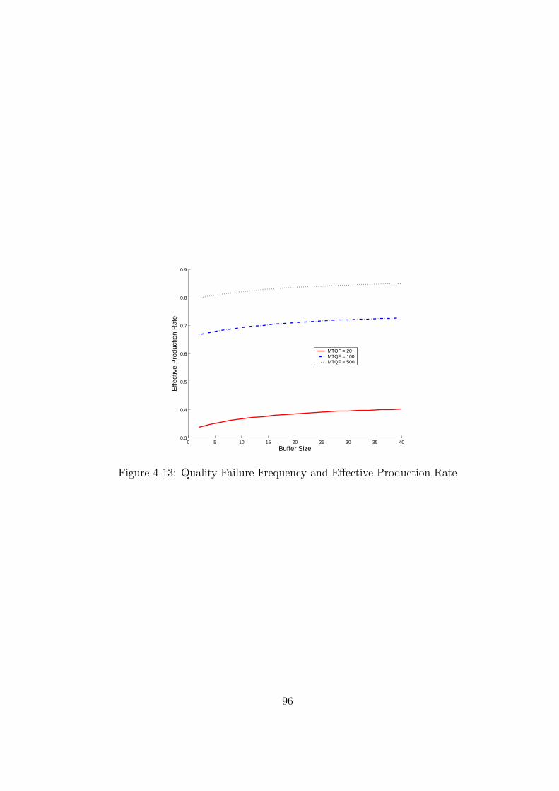
0 5 10 15 20 25 30 35 400.3
0.4
0.5
0.6
0.7
0.8
0.9
Buffer Size
Effe
ctiv
e P
rodu
ctio
n R
ate
MTQF = 20MTQF = 100MTQF = 500
Figure 4-13: Quality Failure Frequency and Effective Production Rate
96

Chapter 5
Long Line Analysis
The two-machine lines of Chapter 3 can be solved analytically, and this means that
fast computer programs can be written to determine performance measures. How-
ever, no such exact analytical solution exists for longer lines. In this chapter, we
describe approximate techniques for long transfer lines with quality failures. Many
different kinds of long manufacturing lines can be analyzed: different topologies (e.g,
tandem, parallel, assembly/disassembly, and closed loops), different quality failures,
different inspection policies and so on. However, in this chapter we focus only on three
non-trivial long manufacturing line tasks to provide fundamental solution methods.
Analysis of various long manufacturing lines is a promising topic for future research.
(See Chapter 7.)
5.1 Introduction
5.1.1 Approximation techniques in long line analysis
Analysis of a line with more than two machines is more difficult than the analysis of
a two-machine system since it leads to a higher state space dimension and increases
the number of boundary conditions. Gershwin and Schick [Gershwin and Schick,
1983] derived an exact solution for the three-machine version of the discrete model.
However, they recognized that it is not extendable to larger systems since it is difficult
to program and ill-behaved.
In case of the continuous model, the analysis of longer lines increases the dimen-
sions of the partial differential equations used in the internal transition equations.
Thus, it appears that obtaining a solution for transfer lines with more than two ma-
97

chines requires approximations. Two different types of approximate techniques have
been proposed so far: decomposition methods and aggregation methods.
The use of decomposition techniques for the analysis of long transfer line was pro-
posed by Zimmern [Zimmern, 1956] for the machines with operation-dependent fail-
ures and by Sevast’yanov [Sevast’yanov, 1962] for the machines with time-dependent
failures.
The idea of the decomposition technique is to decompose a long line into a set of
two-machine lines. Both authors used the continuous model and considered only the
case of homogeneous lines in which all machines have the same repair rates. For the
analysis of the discrete model of long homogeneous lines, approximate decomposition
equations were proposed by Gershwin [Gershwin, 1987]. The decomposition equa-
tions proposed by Gershwin was efficiently solved by the DDX-algorithm, which was
formulated by Dallery, David, and Xie [Dallery et. al, 1989].
Aggregation techniques for the approximate analysis of transfer lines have been
independently proposed by Ancelin and Semery [Ancelin and Semery, 1987], and
Terracol and David [Terracol and David, 1987] in the case of operation-dependent
failures, and De Koster [De Koster, 1987] in the case of time-dependent failures.
The basic idea of the aggregation method is to replace a two-machine-one-buffer
section of the line by a single equivalent machine. Sections of the line are repeatedly
aggregated until only one two-stage system remains. The major deficiency of the ag-
gregation models is that they only account for a unidirectional propagation of events.
For example, when the first two machines are aggregated, there is no accounting for
the effects that downstream blocking might have on the parameters of a previously
aggregated stage. Therefore, the result from aggregating from the first two machines
can be quite different from the result from the aggregating from the last two machines.
The rest of the chapter focuses only on the decomposition methods.
5.1.2 Decomposition techniques for continuous models
without quality failures
For two-machine lines, we can find an exact solution to calculate performance mea-
sures. However, for a long line, it appears to be impossible to find such a solution.
Therefore, an approximation technique is needed. The decomposition technique is the
most popular approximation technique that decomposes the K machine line L into a
set of K−1 two-machine lines L(i) (i = 1, 2, ..., K−1). Each line L(i) is composed of
98

Figure 5-1: Decomposition of a four-machine line into three two-machine lines
an upstream machine Mu(i) and a downstream machine Md(i), separated by a buffer
B(i). This decomposition is illustrated in Figure 5-1 for a four-machine line.
The principle of the decomposition is that the behavior of the material flow in
buffer B(i) closely matches that of the flow in buffer Bi of line L. Machine Mu(i)
represents the part of the line L upstream of Bi and machine Md(i) represents the
part of the line L downstream from Bi.
Decomposition techniques for continuous long lines with operation dependent fail-
ure is more complex than other models (e.g., a deterministic processing time long line)
since it assumes different machine speeds, and the speeds of machines can be slowed
down due to partial blockage and partial starvation. A decomposition technique for a
continuous long line with different operation speeds and operation dependent failures
was first proposed by Glassey and Hong [Glassey and Hong, 1993]. Another method
was developed by Burman [Burman, 1995].
The Accelerated DDX algorithm (ADDX), which was formulated by Burman [Bur-
man, 1995], converges faster and gives more accurate estimates than Glassey and
Hong’s algorithm. The algorithm works as follows:
(1) Initialization
Provide the following initial guesses for the parameters of each two-stage line:
pu(i) = pi
99
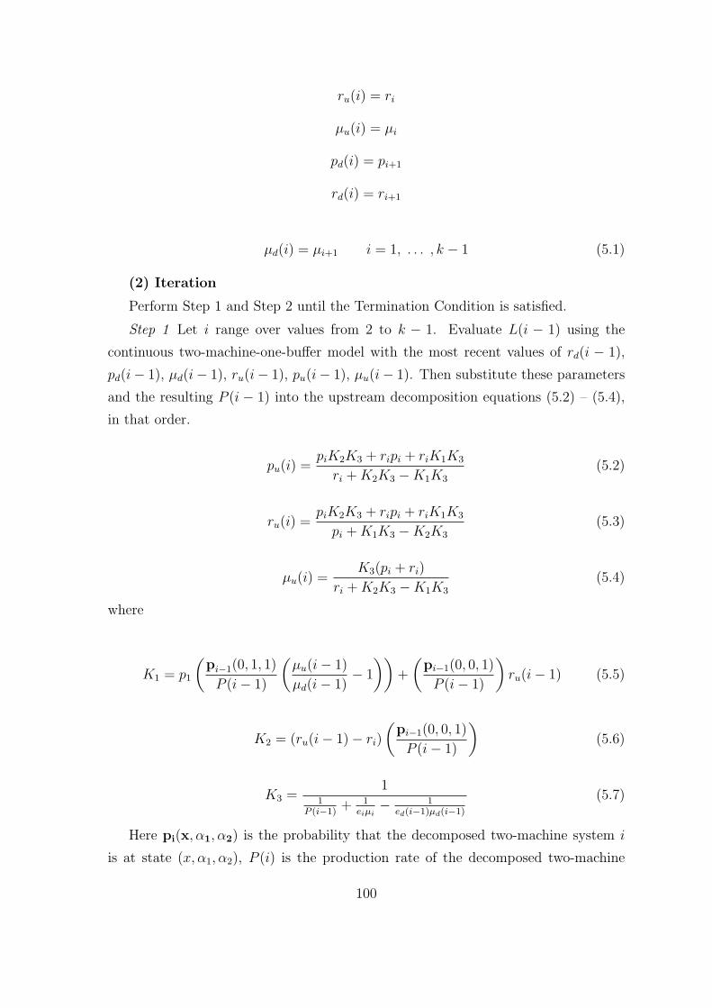
ru(i) = ri
µu(i) = µi
pd(i) = pi+1
rd(i) = ri+1
µd(i) = µi+1 i = 1, . . . , k − 1 (5.1)
(2) Iteration
Perform Step 1 and Step 2 until the Termination Condition is satisfied.
Step 1 Let i range over values from 2 to k − 1. Evaluate L(i − 1) using the
continuous two-machine-one-buffer model with the most recent values of rd(i − 1),
pd(i− 1), µd(i− 1), ru(i− 1), pu(i− 1), µu(i− 1). Then substitute these parameters
and the resulting P (i − 1) into the upstream decomposition equations (5.2) – (5.4),
in that order.
pu(i) =piK2K3 + ripi + riK1K3
ri + K2K3 −K1K3
(5.2)
ru(i) =piK2K3 + ripi + riK1K3
pi + K1K3 −K2K3
(5.3)
µu(i) =K3(pi + ri)
ri + K2K3 −K1K3
(5.4)
where
K1 = p1
(pi−1(0, 1, 1)
P (i− 1)
(µu(i− 1)
µd(i− 1)− 1
))+
(pi−1(0, 0, 1)
P (i− 1)
)ru(i− 1) (5.5)
K2 = (ru(i− 1)− ri)
(pi−1(0, 0, 1)
P (i− 1)
)(5.6)
K3 =1
1P (i−1)
+ 1eiµi
− 1ed(i−1)µd(i−1)
(5.7)
Here pi(x, α1, α2) is the probability that the decomposed two-machine system i
is at state (x, α1, α2), P (i) is the production rate of the decomposed two-machine
100
system i, and ei is the isolated production rate of the two-machine line.
Step 2 Let i range over values from k − 2 to 1. Evaluate L(i + 1) using the
continuous two-machine-one-buffer model with the most recent values of rd(i + 1),
pd(i + 1), µd(i + 1), ru(i + 1), pu(i + 1), µu(i + 1). Then substitute these parameters
and the resulting P (i+1) into the downstream decomposition equations (5.8) – (5.10).
pd(i) =pi+1K5K6 + ri+1pi+1 + ri+1K4K6
ri+1 + K5K6 −K4K6
(5.8)
rd(i) =pi+1K5K6 + ri+1pi+1 + ri+1K4K6
pi+1 + K4K6 −K5K6
(5.9)
µd(i) =K6(pi+1 + ri+1)
ri+1 + K5K6 −K4K6
(5.10)
where
K4 = pi+1
(pi+1(Ni+1, 1, 1)
P (i + 1)
)(µd(i + 1)
µu(i + 1)− 1
)+
(pi+1(Ni+1, 1, 0)
P (i + 1)
)rd(i+1) (5.11)
K5 = (rd(i + 1)− ri+1) +
(pi+1(Ni+1, 1, 0)
P (i + 1)
)(5.12)
K6 =1
1P (i+1)
+ 1ei+1µi+1
− 1eu(i+1)µu(i+1)
(5.13)
(3) Termination Condition Terminate the algorithm when
‖P (i)− P (1)‖ (5.14)
is smaller than a pre-defined small number ε.
5.2 Long line analysis case 1
5.2.1 Introduction
Many different kinds of long manufacturing lines with quality and operational failures
can be analyzed: different topologies, different quality failures, different inspection
policies, and so on. However, there has been no analytical model of these in the
101

literature. In this thesis, we try to take the first and fundamental research step in
building analytic models of long manufacturing lines with quality and operational
failures, by focusing only on three non-trivial long manufacturing line tasks. Analysis
of various long manufacturing lines is a promising topic for future research. (See
Chapter 7.)
M 1
B 1
M 2
M 3
M 4
B 2
B 3
Inspection
Figure 5-2: The first long line analysis task
The first task is the ubiquitous inspection case illustrated in Figure 5-2. This
is the most fundamental but non-trivial model for the long line analysis since the
manufacturing line is long (i.e., more than two machines) and the machines have
both quality and operational failures. In this case, we assume that every machine
undergoes both quality failures and operational failures, and inspection is done at
every operation. More detailed assumptions of the case are as follows:
• Each machine has both operational failures and quality failures.
• Each operation works on different features (e.g., holes, grooves). Thus, quality
failures at an operation do not influence the quality of other operations.
• Inspection at machine Mi can detect defective features made by Mi, not others.
• There is no scrap or rework in the line; defective parts are marked, and scrapped
or reworked later.
5.2.2 Solution method
Transformation technique
Since machines with quality and operational failures have five parameters, µi, ri, pi, gi,
and fi, the analysis of a K-machine line with quality failures requires equations for
10(K − 1) pseudo-machine parameters and a efficient algorithm to solve them.
102

For the ubiquitous inspection case, quality failures at an operation do not influence
the quality of other operations because of the assumption that each operations works
on different features. As a result, gi is independent of other machines’ parameters.
Therefore, we have
gu(i) = gi
gd(i) = gi+1. (5.15)
Another fundamental assumption of the model is that inspection can only identify
bad features made by its own operation. Therefore, for each decomposed line L(i),
(i = 1, 2, ...K − 1) the incoming parts from upstream machines are treated as non-
defective since the inspections at the decomposed line L(i) can not detect defective
parts from the upstream machines. In addition, outgoing defective parts from L(i) are
not detected by the inspections at downstream machines. Thus, fi is also independent
of other machines’ parameters. Therefore, we get
fu(i) = fi
fd(i) = fi+1. (5.16)
4(K − 1) equations are developed from equations (5.15) and (5.16). The remain-
ing 6(K − 1) equations are for the determination of µu(i), µd(i), ru(i), rd(i), pu(i),
and pd(i), which are the parameters for machines with operational failures only. To
determine these parameters, we propose that three-state-machines (state 1, state -1,
and state 0) can be approximated by two-state-machines (state 1’ and state 0), as
depicted in Figure (5-3).
Stopped Operating
1 -1 0
p 3st
1' 0
g 3st f
3st
r 3st
p 2st
r 2st
Figure 5-3: Three-state-machine and corresponding two-state-machine
103
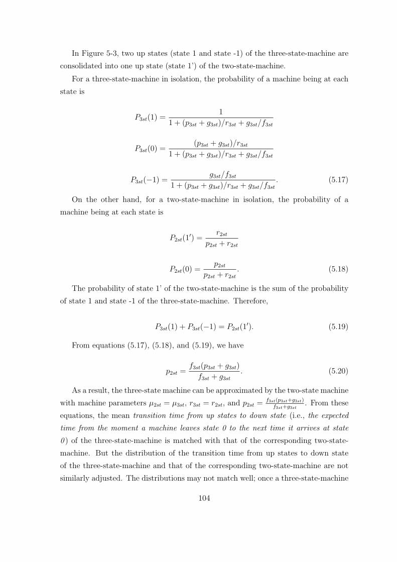
In Figure 5-3, two up states (state 1 and state -1) of the three-state-machine are
consolidated into one up state (state 1’) of the two-state-machine.
For a three-state-machine in isolation, the probability of a machine being at each
state is
P3st(1) =1
1 + (p3st + g3st)/r3st + g3st/f3st
P3st(0) =(p3st + g3st)/r3st
1 + (p3st + g3st)/r3st + g3st/f3st
P3st(−1) =g3st/f3st
1 + (p3st + g3st)/r3st + g3st/f3st
. (5.17)
On the other hand, for a two-state-machine in isolation, the probability of a
machine being at each state is
P2st(1′) =
r2st
p2st + r2st
P2st(0) =p2st
p2st + r2st
. (5.18)
The probability of state 1’ of the two-state-machine is the sum of the probability
of state 1 and state -1 of the three-state-machine. Therefore,
P3st(1) + P3st(−1) = P2st(1′). (5.19)
From equations (5.17), (5.18), and (5.19), we have
p2st =f3st(p3st + g3st)
f3st + g3st
. (5.20)
As a result, the three-state machine can be approximated by the two-state machine
with machine parameters µ2st = µ3st, r3st = r2st, and p2st = f3st(p3st+g3st)f3st+g3st
. From these
equations, the mean transition time from up states to down state (i.e., the expected
time from the moment a machine leaves state 0 to the next time it arrives at state
0 ) of the three-state-machine is matched with that of the corresponding two-state-
machine. But the distribution of the transition time from up states to down state
of the three-state-machine and that of the corresponding two-state-machine are not
similarly adjusted. The distributions may not match well; once a three-state-machine
104

gets to state 1, it has two paths to move to state 0: directly to state 0 with the
rate of p, or through state -1 with the rate of g and then to state 0 with the rate f .
However, the corresponding two-state-machine has only one path to get to state 0.
Therefore, the validity of the approximation depends on whether the distribution of
the transition time from up states to down state of the three-state-machine follows
closely that of the two-state-machine, which is an exponential distribution.
To check this, a simple simulation model of a three-state-machine is developed
and the transition times from up states to down state are recorded. For statistical
significance,1,000,000 cycles of run were used.
Figure 5-4: Distribution of transition time from up states to down state: three-statemachines
Figure 5-4 represents the observed distributions of the transition times for two
different parameter settings where operational failures and quality failures take place
equally frequently. The horizontal axis represents the transition time and the vertical
axis represents the corresponding probability in a logarithmic scale. Both cases in
Figure 5-4 show a close to linear relationship between transition times and the cor-
responding probabilities in logarithmic scales. This means that the transition time
closely follows the exponential distribution.
The equivalent two-state-machine gives the total production rate and average
inventory. But the effective production rate should be estimated indirectly since the
two-state-machine can not tell the difference between ‘good’ state and ‘bad’ state.
Since there is no scrap in the system, the yield of a machine is P3st(1)P3st(1)+P3st(−1)
=f3st
f3st+g3st. For multiple machine lines, the system yield becomes a product of the
105

individual yields. Thus, the effective production rate can be calculated by multiplying
the system yield by the total production rate.
-5.00%
-4.00%
-3.00%
-2.00%
-1.00%
0.00%
1.00%
2.00%
3.00%
4.00%
5.00%
1
7
13
19
25
31
37
43
49
55
61
67
73
79
85
91
97
Case Number
% e
rror o
f P
T
Figure 5-5: 3-state-machine vs. 2-state-machine - comparison of PT
-5.00%
-4.00%
-3.00%
-2.00%
-1.00%
0.00%
1.00%
2.00%
3.00%
4.00%
5.00%
1
7
13
19
25
31
37
43
49
55
61
67
73
79
85
91
97
Case Number
% e
rror o
f P
E
Figure 5-6: 3-state-machine vs. 2-state-machine - comparison of PE
Figure 5-7: 3-state-machine vs. 2-state-machine - comparison of Inv
The performance measures of the 2M1B system with the three-state-machines and
the corresponding two-state-machines are compared in Figures 5-5, 5-6, and 5-7. By
changing machines and buffer parameters, 100 cases are generated, and % errors are
plotted in the vertical axis. The parameters for these cases are given in Appendix
106

A. The average absolute errors in the total production rate, the effective production
rate, and the average inventory are 0.34 %, 0.68%, and 1.07%, respectively.
Analysis procedure
The four-machine ubiquitous inspection case, presented in Figure 5-2, can be analyzed
by using the following procedure:
• Step 1 : Calculate the system yield
Ysys =f1
f1 + g1
× f2
f2 + g2
× f3
f3 + g3
× f4
f4 + g4
.
• Step 2 : Transform the original line L with 3-state-machines into an equivalent
line L′ with 2-state-machines by setting
– µ′i = µi, r′i = ri, p′i = fi(pi+gi)fi+gi
(i = 1, 2, 3, 4).
– N ′i = Ni (i = 1, 2, 3).
• Step 3 : The total production rate and average inventory levels for Bi (i = 1, 2, 3)
of the 2-state-machines line L′ is calculated from ADDX algorithm.
• Step 4 : Evaluate the effective production rate by multiplying the system yield
by the total production rate.
The same procedure can be used for the analysis of a general K-machine line.
5.2.3 Performance Evaluation
Figures 5-8, 5-9, and 5-10 illustrate the comparison of the performance measures
of a large number of four-machine lines with ubiquitous inspections, between the
decomposition algorithm result and simulation result. By choosing machine and buffer
parameters, 50 cases are generated, and % errors are plotted on the vertical axes. The
parameters used for these cases are given in Appendix B. The average absolute errors,
which is the average of the absolute value of the % errors, are presented in Table 5.1.
As observed in the two-machine lines, (Figures 3-26, 3-27, and 3-28), the estimate of
total production rate shows less error than that of the effective production rate. The
observation that the production rates estimates are better than average buffer levels
is consistent with the rest of literature [Dallery and Gershwin, 1992], [Burman, 1995].
107

Table 5.1: Average absolute errors in long line analysis case 1
PT PE WIP Inv1 Inv2 Inv3
Average absolute error (%) 0.37 0.64 3.41 5.46 4.51 2.34
Figure 5-8: Validation – total production rate and effective production rate
Figure 5-9: Validation – WIP (Work-In-Process) and average inventory at B1
108

Figure 5-10: Validation – average inventory at B2 and B3
5.3 Long Line Analysis Case 2
5.3.1 Introduction
The second long manufacturing line analysis task is an extended quality information
feedback (EQIF ) case with four machines as illustrated in Figure 5-11. This is an
extension of the 2M1B quality information feedback model to a longer line. This is
a good approximation of a real situation where operations in the manufacturing line
are reliable in terms of quality, whereas incoming raw material causes major quality
problems, and the defect in the raw material can only identified at the end of line.
Assumptions of the model are as follows:
M 1
B 1
M 2
M 3
M 4
B 2
B 3
Operational Failures + Quality Failures
Inspection
Operational Failures
Figure 5-11: The second long line analysis task
• The first machine (M1) has both operational failures and quality failures.
• The other machines have only operational failures.
• The only inspection is located at the end of line and it can detect non-conformities
made by M1.
109
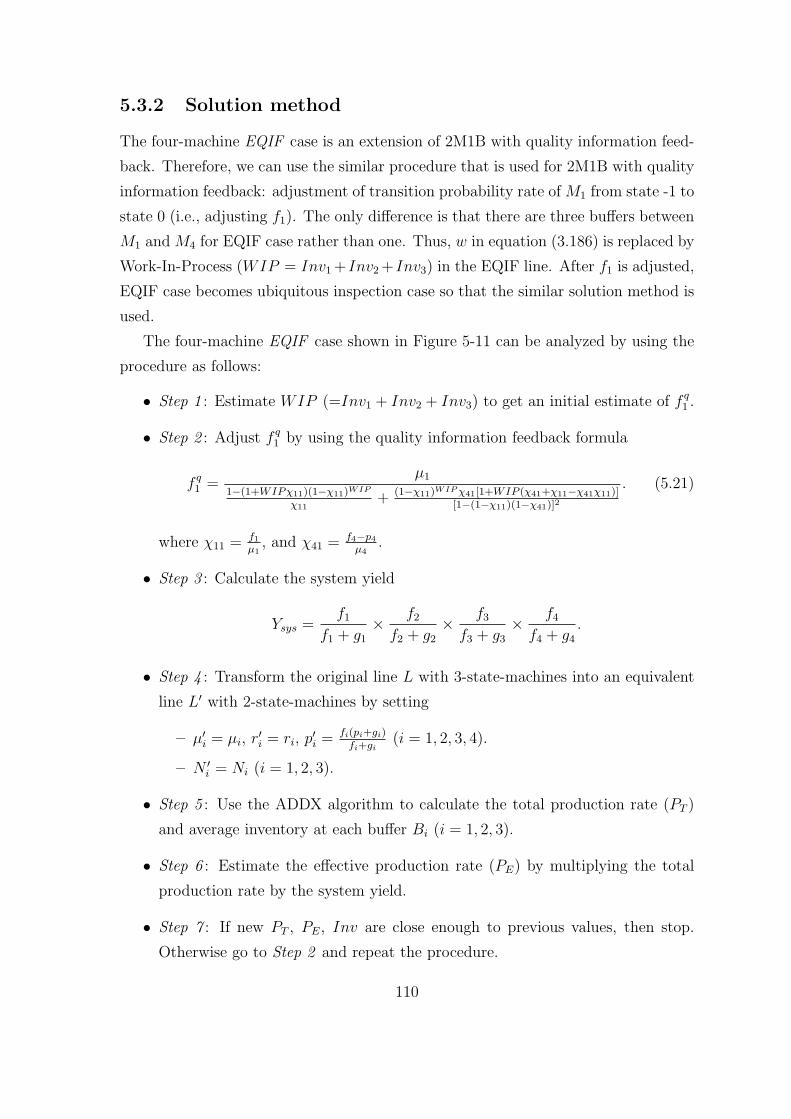
5.3.2 Solution method
The four-machine EQIF case is an extension of 2M1B with quality information feed-
back. Therefore, we can use the similar procedure that is used for 2M1B with quality
information feedback: adjustment of transition probability rate of M1 from state -1 to
state 0 (i.e., adjusting f1). The only difference is that there are three buffers between
M1 and M4 for EQIF case rather than one. Thus, w in equation (3.186) is replaced by
Work-In-Process (WIP = Inv1 + Inv2 + Inv3) in the EQIF line. After f1 is adjusted,
EQIF case becomes ubiquitous inspection case so that the similar solution method is
used.
The four-machine EQIF case shown in Figure 5-11 can be analyzed by using the
procedure as follows:
• Step 1 : Estimate WIP (=Inv1 + Inv2 + Inv3) to get an initial estimate of f q1 .
• Step 2 : Adjust f q1 by using the quality information feedback formula
f q1 =
µ1
1−(1+WIPχ11)(1−χ11)WIP
χ11+ (1−χ11)WIP χ41[1+WIP (χ41+χ11−χ41χ11)]
[1−(1−χ11)(1−χ41)]2
. (5.21)
where χ11 = f1
µ1, and χ41 = f4−p4
µ4.
• Step 3 : Calculate the system yield
Ysys =f1
f1 + g1
× f2
f2 + g2
× f3
f3 + g3
× f4
f4 + g4
.
• Step 4 : Transform the original line L with 3-state-machines into an equivalent
line L′ with 2-state-machines by setting
– µ′i = µi, r′i = ri, p′i = fi(pi+gi)fi+gi
(i = 1, 2, 3, 4).
– N ′i = Ni (i = 1, 2, 3).
• Step 5 : Use the ADDX algorithm to calculate the total production rate (PT )
and average inventory at each buffer Bi (i = 1, 2, 3).
• Step 6 : Estimate the effective production rate (PE) by multiplying the total
production rate by the system yield.
• Step 7 : If new PT , PE, Inv are close enough to previous values, then stop.
Otherwise go to Step 2 and repeat the procedure.
110
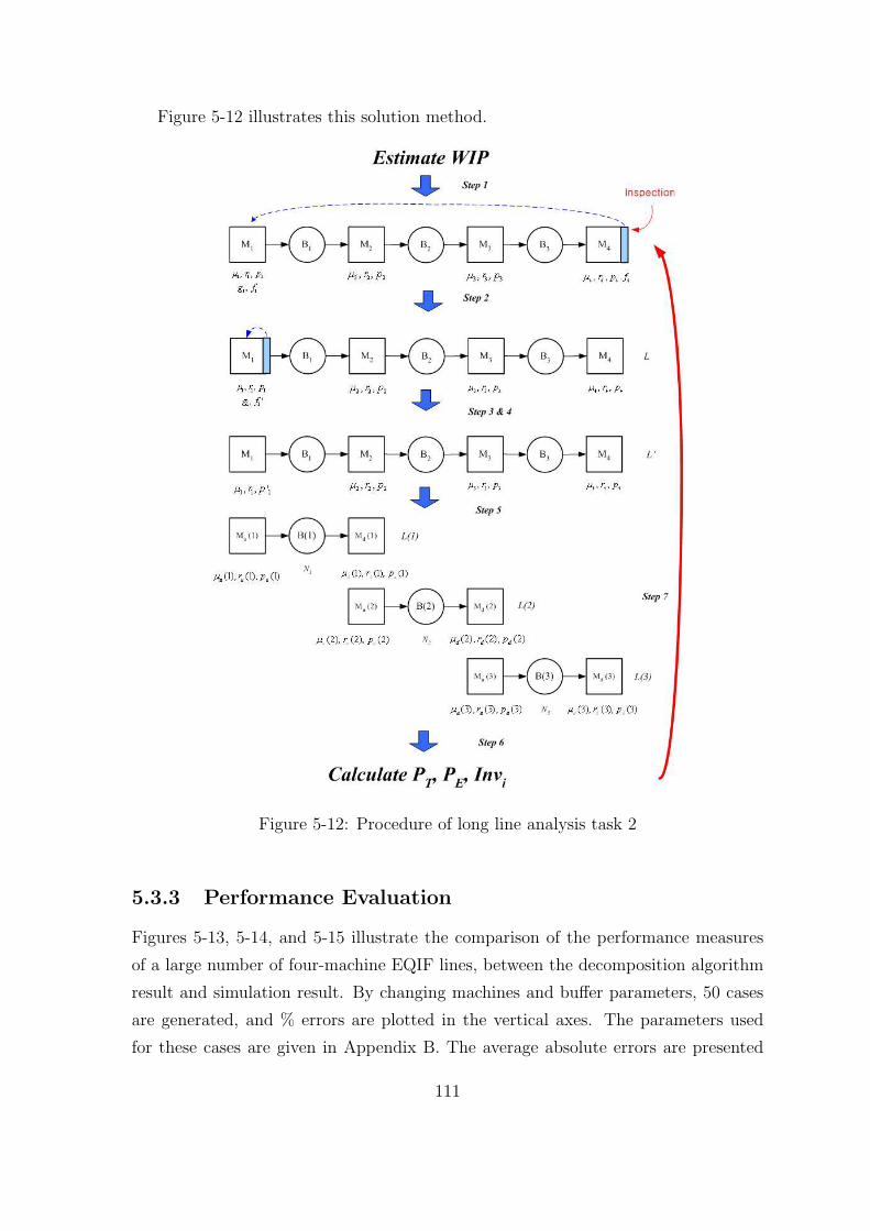
Figure 5-12 illustrates this solution method.
Figure 5-12: Procedure of long line analysis task 2
5.3.3 Performance Evaluation
Figures 5-13, 5-14, and 5-15 illustrate the comparison of the performance measures
of a large number of four-machine EQIF lines, between the decomposition algorithm
result and simulation result. By changing machines and buffer parameters, 50 cases
are generated, and % errors are plotted in the vertical axes. The parameters used
for these cases are given in Appendix B. The average absolute errors are presented
111

in Table 5.2. As observed in the two-machine lines and the ubiquitous inspection
case, the estimate of total production rate shows less error than that of the effective
production rate. The observation that the production rates estimates are better than
average buffer levels is consistent with 2M1B systems and the ubiquitous inspection
case. Note that performance estimates of EQIF case are slightly worse than these
of ubiquitous inspection case since the quality information feedback equation is an
approximate formula as discussed in Chapter 3.
Table 5.2: Average absolute errors in long line analysis case 2
PT PE WIP Inv1 Inv2 Inv3
Average absolute error (%) 0.52 1.02 3.47 5.16 5.56 2.43
Figure 5-13: Validation - PT and PE
Figure 5-14: Validation - WIP and Average Inventory at B1
112

Figure 5-15: Validation - Average Inventory at B2 and B3
5.4 Long Line Analysis Case 3
5.4.1 Introduction
Due to the cost of inspection stations, factories are often designed so that multiple
inspections are performed at a small number of stations. The inspection stations are
usually located at the end of a (sub) line to guarantee that outgoing parts are defect-
free. This is a typical example of a multiple quality information feedback (MQIF )
case, which is illustrated in Figure 5-16. The assumptions of the model are as follows:
Inspection
M 1
B 1
M 2
M 3
M 4
B 2
B 3
Operational Failures + Quality Failures
Figure 5-16: The third long line analysis task
• All the machines have both operational failures and quality failures.
• The only inspection is located at the end of line, and it can detect non-conformities
made by any of the machines (M1, M2, M3, and M4).
• Each operation works on different features. Quality failures at an operation do
not influence the quality of other operations.
113

• There is no scrap in the line; defective parts are marked and reworked later.
5.4.2 Solution method
The four-machine MQIF case shown in Figure 5-16, is an extension of EQIF case
in a sense that multiple quality information feedback loops exist. Therefore, we can
repeat the same procedure that is used for EQIF case for each of the loop. The only
difference is that w in equation (3.186) is replaced by:
• Inv1 + Inv2 + Inv3 for the adjustment of f1.
• Inv2 + Inv3 for the adjustment of f2.
• Inv3 for the adjustment of f3.
The four-machine MQIF case can be analyzed by using the procedure as follows:
• Step 1 : Estimate the average inventory of each buffer (Inv1, Inv2, and Inv3).
• Step 2 : Adjust f qi (i = 1, 2, 3) by using the QIF formula:
f qi =
µi
1−(1−χii)wi
χii− wi(1− χii)wi + (1−χii)wiχ4i[(wi+1)−wi(1−χii)(1−χ4i)]
[1−(1−χii)(1−χ4i)]2
where χii = fi
µi, χ4i = f4−p4
µ4, w1 = Inv1 + Inv2 + Inv2, w2 = Inv2 + Inv3, and
w3 = Inv3.
• Step 3 : Calculate the system yield
Ysys =f1
f1 + g1
× f2
f2 + g2
× f3
f3 + g3
× f4
f4 + g4
.
• Step 4 : Transform the original line L with 3-state-machines into an equivalent
line L′ with 2-state-machines by setting
– µ′i = µi, r′i = ri, p′i = fi(pi+gi)fi+gi
(i = 1, 2, 3, 4).
– N ′i = Ni (i = 1, 2, 3).
• Step 5 : Use the ADDX algorithm to calculate the total production rate (PT )
and average inventory at each buffer Bi (i = 1, 2, 3).
114

Figure 5-17: Procedure of long line analysis task 3
115

• Step 6 : Estimate the effective production rate (PE) by multiplying the total
production rate by the system yield.
• Step 7 : If the new PT , PE, Inv are close enough to their previous values, then
stop. Otherwise go to Step 2 and repeat the procedure..
Figure 5-17 illustrates this solution method.
5.4.3 Performance Evaluation
Figures 5-18, 5-19, and 5-20 illustrate the comparison of the performance measures
of a large number of four-machine MQIF lines, between the decomposition algorithm
result and simulation result. By changing machine and buffer parameters, 50 cases
are generated, and % errors are plotted in the vertical axes. The parameters used
for these cases are given in Appendix B. The average absolute errors are presented in
Table 5.3.
As observed in the two-machine lines, the ubiquitous inspection case, and the
EQIF case, the estimate of total production rate shows less error than that of the
effective production rate. The observation that the production rates estimates are
better than average buffer levels is consistent with the other cases. Note that per-
formance estimates of MQIF case are slightly worse than these of EQIF case since
the approximate quality information feedback equation is used multiple times. This
deterioration of performance estimates suggests that the errors tend to increase as the
manufacturing line gets longer (thus, more quality information feedback loops exist).
Table 5.3: Average absolute errors in long line analysis case 3
PT PE WIP Inv1 Inv2 Inv3
Average absolute error (%) 0.55 1.95 8.62 5.97 4.75 2.76
In this chapter, we propose the solution methods for the three non-trivial long
manufacturing line tasks as a first step in analyzing long manufacturing lines with
quality and operational failures. The comparison with simulations show that the
solution methods provide the reliable performance estimates of long manufacturing
lines. Analysis of various long manufacturing lines is a promising topic for future
research. (See Chapter 7.)
116

Figure 5-18: Validation - PT and PE
Figure 5-19: Validation - WIP and average inventory at B1
Figure 5-20: Validation - average inventory at B2 and B3
117

118

Chapter 6
Jidoka
6.1 Jidoka practice in Toyota Production System
A significant portion of the Toyota Production System is traceable to an automatic
loom invented early in the 20th century at Toyota Spinning & Weaving, the parent
company of the Toyota Motors Corporation. The loom was designed to stop working
immediately whenever thread snapped. The principle of stopping an operation when
a problem occurs and preventing the production of defective items is fundamental to
the Toyota Production System. This principle is called jidoka [Togo and Waterman,
1993]. In the Toyota Production System, equipment is designed to detect abnormal-
ities and to stop automatically and immediately whenever they occur. Operators
at assembly lines are provided means of stopping the production flow (andon cords)
whenever they note anything unusual.
Experts in the Toyota Production System argue that the Jidoka practice has
brought several benefits: The most significant of them is that it eliminates the need
for the workers to oversee machine operations. As a result, an operator can handle
multiple machines. It is not unusual that one operator handle 7 to 10 machines in
the Toyota Production System. The man-machine separation led to significant direct
labor cost saving and made it possible to use cellular manufacturing systems.
Another widely mentioned advantage of “stopping a line when abnormalities take
place” is that it motivates kaizen (continuous improvement) since operators can
clearly see the painful outcome of producing defects: the line stoppage. And it
is easier to find the root cause of a problem right after the problem takes place.
Through the use of systematic ways of resolving problems (e.g. asking “Why?” five
119

times) which are widely accepted in Toyota, operators’ learning speed accelerated [Fu-
jimoto, 1999]. It has been known that operators’ learning can significantly improve
productivity and quality [Henderson, 1982], [Sandberg, 1995].
The other benefit of jidoka that Toyota Production System advocates claim is
that it prevents the waste that would result from producing a series of defective
items. Therefore, jidoka is considered to be a means to improve quality and increase
productivity at the same time [Toyota Motors Corporation, 1996], [Monden, 1998].
When quality failures are persistent, in which once a bad part is produced, all subse-
quent parts will be bad until the machine is repaired, catching bad parts and stopping
the machine as soon as possible is the best way to maintain high quality and pro-
ductivity. This is the case with breakage of thread, which caused the invention of
jidoka practice a century ago at Toyota Spinning & Weaving [Togo and Waterman,
1993]. On the other hand, defects are often from Bernoulli quality failures in which
the quality of each part is independent of the others. In this case, there is no benefit
to stop a machine that has made a bad part because there is no reason to believe that
upcoming parts are bad; thus stopping the machine would reduce the number of bad
parts in the future. In this case, therefore, stopping the operation does not improve
quality but it reduces productivity by losing working time.
In reality, most of machines have multiple-yield quality failures. When a machine
is in good shape and operating without any assignable cause variations (in control
or high-quality state), it may produce a defective part with a very small probability,
not because of any internal change in the machine but because of random external
perturbations. However, when a machine is operating under assignable cause varia-
tions (out of control or low-quality state), it is likely that many of upcoming parts
are bad. In this situation, the optimal stopping policy is, therefore to stop the ma-
chine only if the machine is in low quality state. But in many cases it is not easy to
tell whether the machine is in high-quality state or low-quality-state (in other words,
whether quality failure is from random variation or assignable cause variation) with
one sample. Matters even get more complicated when inspection is not reliable.
In this case, what would be an optimal stopping policy? Qualitatively speaking,
stopping immediately after detecting a bad part may not be optimal when Bernoulli
quality failures is more frequent, mean time to repair (MTTR) is long and inspection
is not reliable. Analytic models developed in Chapter 3 can give more precise and
quantitative answers to the question.
120

6.2 Modeling of Multiple-Yield Quality Failures
6.2.1 Multiple-Yield Quality Failures
Jidoka practice means stopping a machine or a manufacturing line immediately when
a defective part is made. Basically, people adopt jidoka assuming that inspection is
100% reliable and that all the defects are from persistent quality failures. In that
case, it is clear that jidoka improves quality and productivity at the same time. But
when there are Bernoulli quality failures and multiple-yield quality failures, there is
no guarantee that subsequent parts will be defective after finding a non-conformity.
In this case, it may be better to stop a machine when the machine produces two
defective parts in a row since it is not likely to have two Bernoulli-type quality failures
consecutively. To check the optimality of the jidoka stopping policy, we need to
model multiple-yield quality failures. Figure 6-1 shows a modified state definition of
a machine for the simplest multiple-yield quality failure model:
• State 1: The machine is in good shape and operating without any assignable
cause variations. It may produce defective parts with probability 1−π(1), which
is close to 0, due to random variations.
• State -1: The machine is operating under assignable cause variations and pro-
ducing bad parts with probability 1 − π(−1), which is close to 1. But the
operator does not know this yet.
• State 0: The machine is not operating.
Therefore, π(1) is the yield of a machine when the machine is at state 1. And
π(−1) is the yield of the machine when it is at state -1. When the machine is either in
state 1 or -1, it can be stopped for two reasons: operational failures with probability
rate pj and quality failures with transition rate qj (j = −1, 1). Here, 1/qj is a Mean
Time to Stop due to Quality failures (MTSQ) which depends on frequency of quality
failures, inspection reliability, and machine stopping policies. Since we assume that
the occurrence of operational failures is independent of machine states, p1 = p(−1) = p.
The transition from state 1 to state 0 occurs with probability rate s = p1 + q1,
and the transition from state -1 to state 0 occurs with probability rate f = p−1 + q−1.
A system that has persistent quality failures only is a special case where:
• π(1) = 1 and π(−1) = 0.
121
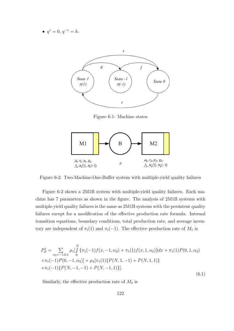
• q1 = 0, q−1 = h.
Figure 6-1: Machine states
Figure 6-2: Two-Machine-One-Buffer system with multiple-yield quality failures
Figure 6-2 shows a 2M1B system with multiple-yield quality failures. Each ma-
chine has 7 parameters as shown in the figure. The analysis of 2M1B systems with
multiple-yield quality failures is the same as 2M1B systems with the persistent quality
failures except for a modification of the effective production rate formula. Internal
transition equations, boundary conditions, total production rate, and average inven-
tory are independent of πi(1) and πi(−1). The effective production rate of M1 is
P 1E =
∑α2=−1,0,1
µ1[N∫0
{π1(−1)f(x,−1, α2) + π1(1)f(x, 1, α2)}dx + π1(1)P (0, 1, α2)
+π1(−1)P (0,−1, α2)] + µ2[π1(1){P (N, 1,−1) + P (N, 1, 1)}+π1(−1){P (N,−1,−1) + P (N,−1, 1)}].
(6.1)
Similarly, the effective production rate of M2 is
122

P 2E =
∑α1=−1,0,1
µ2[N∫0
{π2(−1)f(x, α1,−1) + π2(1)f(x, α1, 1)}dx + π2(−1)P (N, α1,−1)
+π2(1)P (N,α1, 1)] + µ1[π2(1){P (0,−1, 1) + P (0, 1, 1)}+π2(−1){P (0,−1,−1) + P (0, 1,−1)}].
(6.2)
Equations (6.1) and (6.2) become equations (3.92) and (3.93) when πi(1) = 1 and
πi(−1) = 0.
6.2.2 Modeling of Stopping Policies
As discussed earlier, we define qji as the probability rate that a machine i (Mi) is
stopped due to quality failures when Mi is in state j (j = −1, 1). The value of qji
depends on frequency of quality failures, inspection reliability, and stopping policies.
Jidoka is based on 100% reliable inspection, and the frequency of quality failures is
intrinsic to operations. Therefore, we only need to consider stopping policies to check
the optimality of jidoka practice. For the sake of simplicity, we consider two different
stopping policies:
• Policy 1 : Stop a machine when a bad part is produced.
• Policy 2 : Stop a machine when two bad parts are produced consecutively.
Stopping policy 1 is the policy that is incorporated in jidoka practice. If the per-
sistent quality failures are the only quality failures, stopping a machine immediately
after it produces a defect is better than stopping with two consecutive defects. But,
in the case of Bernoulli quality failures and multiple-yield quality failures, the per-
formance of the two stopping policies depends on many factors (e.g. g, π(1), r, and
others).
Modeling of stopping policy 1
The probability of making a bad part when Mi is in state j is 1−πi(j). For stopping
policy 1, we assume 100% reliable inspection and an immediate stoppage of a machine
after a detection of a defect. As a result, the MTSQ (= 1
qji
) is the same as the mean
time for a quality failure to occur:
123

1
qji
=1
µi
[(1−πi(j))+2(1−πi(j))πi(j)+3(1−πi(j))(πi(j))2+...] =
1
µi(1− πi(j)), (j = −1, 1).
(6.3)
Here, 1µi
is a cycle time. Therefore,
qji = µi(1− πi(j)), (j = −1, 1) (6.4)
The 2M1B systems with multiple-yield quality failures and stopping policy 1 can
be analyzed with the 2M1B systems developed in Chapter 3 with some modifications:
• Modify machine parameters pi with si = pi + µi(1 − πi(1)) and fi with fi =
pi + µi(1− πi(−1)). Other parameters, gi, ri, N (i = 1, 2), are unchanged.
• P 1E and P 2
E are calculated from equations (6.1) and (6.2).
Modeling of stopping policy 2
For stopping policy 2, MTSQ is an expected time for two quality failures to occur in
a row. Therefore, MTSQ can be estimated through the expected time to absorption
problem. [Bertsekas and Tsitsiklis, 2002].
In Figure 6-3, there are three states:
• State 0 : There is no defect in the last two products.
• State 1 : There is one defect in the last two products.
• State 2 : There are two defects in the last two products.
β is the probability of producing a good part. When two bad parts are produced
in a row, the machine is stopped according to stopping policy 2. Therefore, state 2 is
absorbing. If we define vi as the expected times to absorption from a transient state
i, then MTSQ is v0/µi.
We can construct equations for the expected time to absorption problem as follows
[Bertsekas and Tsitsiklis, 2002]:
v0 = (1− β)v1 + βv0 + 1 (6.5)
v1 = βv0 + 1 (6.6)
124
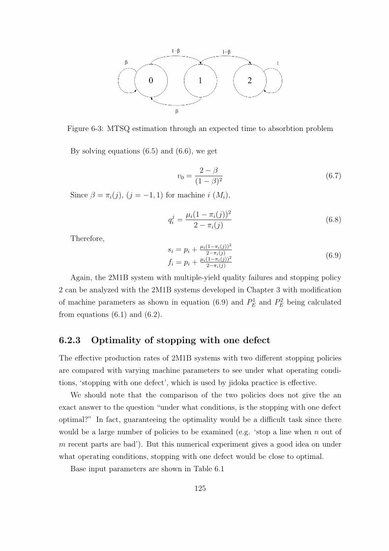
Figure 6-3: MTSQ estimation through an expected time to absorbtion problem
By solving equations (6.5) and (6.6), we get
v0 =2− β
(1− β)2(6.7)
Since β = πi(j), (j = −1, 1) for machine i (Mi),
qji =
µi(1− πi(j))2
2− πi(j)(6.8)
Therefore,
si = pi + µi(1−πi(j))2
2−πi(j)
fi = pi + µi(1−πi(j))2
2−πi(j)
(6.9)
Again, the 2M1B system with multiple-yield quality failures and stopping policy
2 can be analyzed with the 2M1B systems developed in Chapter 3 with modification
of machine parameters as shown in equation (6.9) and P 1E and P 2
E being calculated
from equations (6.1) and (6.2).
6.2.3 Optimality of stopping with one defect
The effective production rates of 2M1B systems with two different stopping policies
are compared with varying machine parameters to see under what operating condi-
tions, ‘stopping with one defect’, which is used by jidoka practice is effective.
We should note that the comparison of the two policies does not give the an
exact answer to the question “under what conditions, is the stopping with one defect
optimal?” In fact, guaranteeing the optimality would be a difficult task since there
would be a large number of policies to be examined (e.g. ‘stop a line when n out of
m recent parts are bad’). But this numerical experiment gives a good idea on under
what operating conditions, stopping with one defect would be close to optimal.
Base input parameters are shown in Table 6.1
125
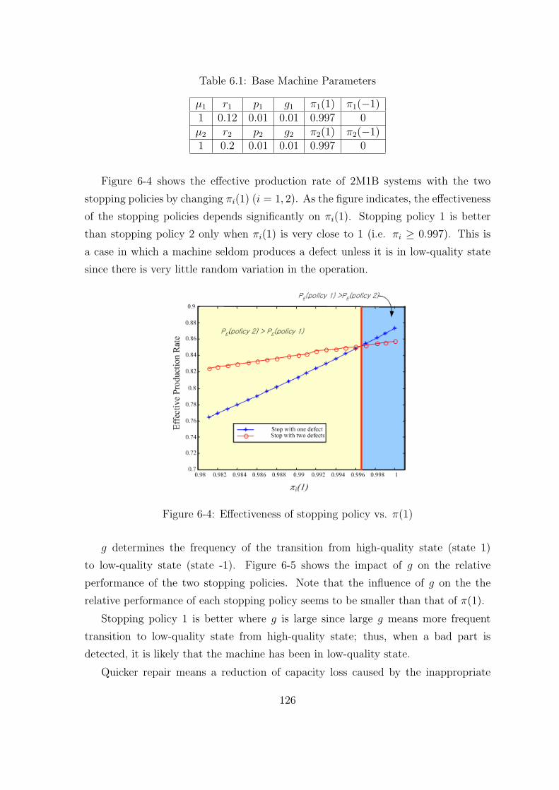
Table 6.1: Base Machine Parameters
µ1 r1 p1 g1 π1(1) π1(−1)1 0.12 0.01 0.01 0.997 0µ2 r2 p2 g2 π2(1) π2(−1)1 0.2 0.01 0.01 0.997 0
Figure 6-4 shows the effective production rate of 2M1B systems with the two
stopping policies by changing πi(1) (i = 1, 2). As the figure indicates, the effectiveness
of the stopping policies depends significantly on πi(1). Stopping policy 1 is better
than stopping policy 2 only when πi(1) is very close to 1 (i.e. πi ≥ 0.997). This is
a case in which a machine seldom produces a defect unless it is in low-quality state
since there is very little random variation in the operation.
Figure 6-4: Effectiveness of stopping policy vs. π(1)
g determines the frequency of the transition from high-quality state (state 1)
to low-quality state (state -1). Figure 6-5 shows the impact of g on the relative
performance of the two stopping policies. Note that the influence of g on the the
relative performance of each stopping policy seems to be smaller than that of π(1).
Stopping policy 1 is better where g is large since large g means more frequent
transition to low-quality state from high-quality state; thus, when a bad part is
detected, it is likely that the machine has been in low-quality state.
Quicker repair means a reduction of capacity loss caused by the inappropriate
126

Figure 6-5: Effectiveness of stopping policy vs. g
Figure 6-6: Effectiveness of stopping policy vs. repair rate
127

stoppage of a machine. Therefore, stopping with one defect outperforms stopping with
two defects in a row, when r is large which is shown in Figure 6-6. More numerical
experiments show that a higher value of πi(1) leads to a higher r value where the
two stopping policies give the same effective production rate. The comparison with
Figures 6-4 and 6-5 reveals that the impact of r on the relative effectiveness of the
two stopping policies is weaker than π(1) and g.
Numerical experiments show that the relative performances of 2M1B systems with
the two stopping policies are insensitive to other machine parameters (e.g. pi, fi, µi,
and πi(−1), i = 1, 2).
Figure 6-7 illustrates the domain of π(1) and g where ‘stopping with one defect’
outperforms ‘stopping with two defects’. Two machine parameters π(1) and g are used
since these are the two major factors that the effective production rate is sensitive
to. Standard process capability used at Toyota is Cp = 1.33, which means more than
99.99% of yield in operations [Monden, 1993]. If we assume that typical value of r
at factories in the automotive industry is around 0.2, and that g is usually less than
0.01, this operating condition is in the domain where ‘stopping with one defect’ is
better as shown in Figure 6-7.
0
0.01
0.02
0.03
0.04
0.05
0.06
0.07
0.08
0.98 0.985 0.99 0.995 1
g
P E (policy 1) > P
E (policy 2)
P E (policy 2) > P E (policy 1)
Toyota plants
Figure 6-7: Comparison of stopping policy and operation range of Toyota plants
In other words, it seems that the stopping policy with jidoka practice is close
to optimal at Toyota plants under the assumption that inspection is reliable. Note
that all the equations are based on the ‘perfectly reliable inspection’ assumption.
When inspection is not reliable, stopping with one defect is less likely be optimal
since it is even not certain whether the machine actually produced nonconformity.
We conclude that jidoka is likely to be optimal when factories are operating under
128

desirable conditions (e.g., high process capability (Cp > 1), infrequent occurrence
of assignable causes, and short repair time). However, more research is needed to
determine the influence of other realistic factors such as imperfect inspection.
129

130
Chapter 7
Future Research
Throughout the thesis work, we have observed the lack of prior research on the
intersection of quality, productivity, and manufacturing systems design. Discussions
with automotive companies have revealed the industry’s strong need for the research
in this field. This thesis lays a cornerstone for the quantitative research in the area
but there still remain many research opportunities. These opportunities are identified
and some promising research strategies are described in this chapter.
7.1 Two-machine-one-buffer systems
7.1.1 Part scrapping at each operation
We have focused on manufacturing systems with no scrapping within the line (i.e.,
scrapping can take place at the end of the line). This is a reasonable assumption for
an automotive assembly line where parts are big and heavy so that removing a part
from the middle of the line is economically infeasible. But scrapping in the middle of
the line may happen frequently in the manufacturing of small parts, such as electronic
parts. In this case, the analytic modeling of the 2M1B systems becomes completely
different. A new state definition may be needed since we need to differentiate good
parts from defective parts in the buffer to scrap the bad ones only. In addition, a
whole new set of internal transition equations and boundary conditions would have
to be developed. The change in the buffer level, when the buffer is neither empty nor
full, is no longer infinitesimal during a short time interval when scrapping takes place.
Also, arrival to and departure from the boundaries become more complicated. New
solution methods to solve the internal transition equations and boundary conditions
131
would be needed.
7.1.2 Part rework
In a situation where defective parts are reworked at each operation, correcting the
defects may require some additional operations. Therefore, it may alter the operation
cycle time (i.e., machine speed) temporarily. As a result, the speed of a machine
becomes dependent on the state of the machine. Again, a new set of internal transition
equations, boundary conditions, and a solution method to solve these equations should
be developed.
7.1.3 Correlation among different quality failures
Each quality failure is associated with a specific feature of a part. Throughout this
thesis, we have assumed that each machine works on a different feature. This allows
us to assume that the quality failures of the machines are independent. However, if
a feature is the product of a sequence of operations (e.g., two machines work on the
same hole: the first machine (M1) does a roughing operation and the second machine
(M2) does a finishing operation), quality failures of M2 are influenced by the operation
of M1. In this case, the state of M2 is a function of the state of M1. (i.e., M2 is more
likely to go to state -1 if M1 is in state -1). In addition, the traceability of the root
cause of a quality failure would be an issue; a defective feature made from a sequence
of operation may contain a defect due to any one of the operations in the sequence.
Then, determining which machine to stop for repair would be an important problem.
7.1.4 Reliability of inspection
Typically, testing is an imperfect process. The reliability of an inspection depends on
many factors, including inspection equipment, sampling frequency, sample size, and
others, but completely eliminating the errors in inspection is impossible. There are
two types of errors:
• Type 1 error: errors where the part is good, but the test concludes that it is
defective.
• Type 2 error: errors where the part is defective, but the test concludes that it
is good.
132

In this thesis, 2M1B models include Type 2 errors in inspection; when f is small,
a machine may produce multiple bad parts before it is stopped by operator for repair.
But Type 1 errors are not considered. Including the Type 1 error may need modifi-
cation of the transition rate between state 1 and state 0 or it may need a different
machine state definition.
7.1.5 Productivity reduction due to inspection
In this thesis, we assume that inspection does not consume time. In many cases,
however, inspection is time-consuming and tends to slow down the manufacturing
process. Therefore, adding inspection may not only incur more cost (e.g., floor space,
equipments, and labor) but may also reduce the capacity of the manufacturing system.
The time-consuming inspection problem may be solved simply by adding a machine
whose cycle time corresponds to the inspection time.
7.1.6 Aging
A machine may produce conforming parts with probability π(t). If the machine
were to get progressively out of tune due to tool wear, then π(t) is a decreasing
function of time. This phenomenon is called an aging process, and it is not unusual
in manufacturing processes. The continuous aging process can be approximated with
a machine with numerous discrete states with decreasing yields (π1 > π2 · · · > πN) as
shown in Figure 7-1.
Figure 7-1: Modeling of aging process
133

7.2 Large systems
7.2.1 Topology of manufacturing systems
The modeling and analysis of quality and productivity issues in a manufacturing
system are fundamentally influenced by its topology. Production lines come in widely
different forms: serial lines, assembly/disassembly lines, parallel lines, and closed-loop
systems. Decomposition techniques to analyze these topologies have been developed
for production systems without quality failures [Gershwin, 1994], [Levantesi, 2001].
It is not clear whether the same kind of solution techniques, which are used in this
thesis for the analysis of serial lines, can be applied to analyzing production systems
with different topologies.
A split-merge line illustrated in Figure 7-2 is widely used when operations in the
parallel lines (e.g.,M3) are substantially slower than operations in the serial line (e.g.,
M7). In the parallel lines that are designed to perform identical functions, normal
everyday operation may lead to small amounts of variability in nominally identical
machines, and therefore in the parts produced by those machines. Such variability
may have an effect on quality of products after the end of the line after the parallel
lines merge especially when a high precision assembly or fabrication operation may
follow. Estimating the influence of parallel lines on the quality of products would be
an important research topic.
M1 B1 M2 B2
M3 B3 M4
B5 M7
M5 B4 M6
B6 M8
Figure 7-2: Split-merge line
7.2.2 Location and domain of inspection
Ideally, ubiquitous inspection (i.e., the placement of an inspection station after each
machine) would result in the immediate detection and isolation of quality failures,
simplifying root-cause traceability and minimizing the waste of downstream produc-
tion capacity. However, inspection stations are expensive, in that they consume floor
space, capital, and labor. Therefore, it is necessary to choose the number and loca-
134

tion of inspection stations carefully, so as to place them as sparsely as possible while
meeting quality goals.
An inspection station placed after a certain sequence of machines may be designed
to detect quality failures produced by all the machines in that sequence (Figure 7-3),
or only a subset of them (Figure 7-4), (Figure 7-5). Some features produced by certain
operations may undergo multiple inspections (Figure 7-6). Different configurations of
the inspection domain may require different decomposition procedures. The accuracy
of the long line analysis may significantly depend on the the number, the location,
and the configuration of inspections.
I
Scrap or rework
Figure 7-3: Single downstream inspection
I I
Scrap or rework Scrap or rework
Figure 7-4: Contiguous inspection regions
I I
Scrap or rework Scrap or rework
Figure 7-5: Non-contiguous inspection regions
7.2.3 Behavior of long lines
Through the numerical experiments, the behaviors of 2M1B systems were studied in
Chapter 4. Although much of the qualitative behavior of long manufacturing lines
135

I I
Scrap or rework Scrap or rework
Figure 7-6: Overlapping inspection regions
can be inferred from that of the 2M1B system (e.g., beneficial, harmful, and optimal
buffer cases), there may be some special behaviors of the long lines that can not
be conjectured from the 2M1B systems. Looking for interesting behaviors of the
long lines through conducting numerical experiments is time-consuming since the
number of parameters in the system grows rapidly as the lines get longer (e.g., for K
machine lines, there are 6K−1 machine and buffer parameters). The analytic models
provided in this thesis have substantial advantage over simulation, in searching for
special behavior of the long manufacturing lines due to substantial computation time
savings.
7.3 Optimal manufacturing system design
The optimal design of manufacturing systems is a vast research area in which a
substantial number of papers have been published [Raz, 1986], [Gershwin and Schore,
2000], [Daya and Rahim, 2003]. Under this topic, two major sub-problems have
received significant attentions: the optimal inspection allocation problems, and the
optimal buffer space allocation problems. These two problems have been extensively
studied, but there is a lack of research in their intersection since the two fields have
been considered separate. In the optimal inspection allocation problems, previous
authors have assumed Bernoulli-type quality failures [Raz, 1986]. Therefore, the role
of inspection is to screen out defective parts, not to identify machines in bad states
and fix them. Therefore, the system yield has nothing to do with average inventories
and buffer sizes. In the optimal buffer space allocation problems, no quality failures
are considered; machines are assumed to produce conforming parts and they undergo
operational failures only. However, when persistent or multiple-yield quality failures
exists and quality information feedback is used, the system yields become a function
136

of buffer sizes as demonstrated in Chapter 4. As a result, the optimal inspection
allocation problems and the optimal buffer size allocation problems become coupled and
should be solved simultaneously. The analytical models of serial long lines presented in
Chapter 5 can be used for this end, combined with a proper optimization technique.
7.4 Worker motivation and learning
The design and operation of manufacturing systems may affect the behavior of the
workers on the production line, thereby indirectly influencing the quality and produc-
tivity of the manufacturing system. The relationship between the design of production
lines, and workers’ motivation and learning speed has been out side of the scope in
this thesis. However, there has been significant research conducted on this relation-
ship [Schultz et al., 1998], [Lieberman and Demeester, 1999], [Fujimoto, 1999], [Alles
et al., 2000]. This research suggest that the reduction of inventory leads to an early
detection of quality failures; thus, it facilitates the identification of the root cause of
the problems. This allows people on manufacturing lines to develop a better under-
standing of the manufacturing processes and to feel more motivation for operations
improvement (i.e., kaizen).
In a manufacturing system where manual labor is heavily used, (e.g., assembly
lines), this relationship between the system design and the workers’ behavior becomes
more important. The increase of buffer size in the beneficial buffer case (Figure 4-
2) presented in Chapter 4 may not actually be beneficial (i.e., leading to higher
productivity) in fact, if the detrimental influence of large buffer on workers’ learning
is considered. Stopping with one defect, which is incorporated in the jidoka practice,
might be the optimal stopping policy even for the less desirable operating conditions
described in section 6.2.3 (see Figure 6-7) in the long run, if the workers’ motivation
and learning are taken into consideration.
Most quantitative research on the manufacturing system design has neglected
the human issue. Manufacturing system design principles derived from this kind of
research are useful for designing and operating factories where automated machines
are heavily used (e.g., flexible manufacturing systems). But these principles would be
inappropriate if they are applied to labor intensive factories. Therefore, more holistic
research combining the issue of the interaction between people and manufacturing
system design with quantitative modeling and analysis of manufacturing system is
137

needed.
138

Chapter 8
Conclusion
This thesis takes an essential early research step in analyzing how production system
design, quality, and productivity are inter-related. There was very little quantitative
analytical literature that explores this area, even though the effects of the interaction
are recognized on the plant floor anecdotally.
Throughout the thesis, we identify important differences among types of quality
failures, and develop a new Markov process model for machines with both quality
and operational failures. Based on the single-machine analysis, we present analytic
models, solution techniques, performance evaluations, and validation of two-machine
systems, as well as longer production lines.
Numerical studies using two-machine models show that when the first machine
has quality failures and the inspection occurs only at the second machine, there are
cases in which the effective production rate increases as buffer size increases, and
there are cases in which the effective production rate decreases for larger buffers.
We present various methods of improving quality and productivity, and demonstrate
that the effectiveness of each method is greatly dependent upon the particularities
of factories. Therefore, the need to find the most effective combination of method
in each case is identified, and the usefulness of the quantitative tools developed in
this thesis is shown. We also investigate the effectiveness of jidoka practice, and find
that jidoka is useful only when machines are operating under stable conditions. We
reaffirm the importance of and the urgent need for research in this field, and we
propose promising research directions.
139

140

Bibliography
[1] Alles, M., Amershi, A., Datar, S., and Sarkar, R., “Information and incentive
effects of inventory in JIT production,” Management science, Vol. 46 No. 12
pp.1528 - 1544, December 2000.
[2] Altiok, T., Performance analysis of manufacturing systems,, Springer Verlag,
New York, 1997.
[3] Ammeraal, Leen, STL for C++ programmers John Wiley & Sons, 1997.
[4] Ancelin, B. and Semery, A., “Calcul de la productivite d’une ligne integree de
fabrication: CALIF, une methode analytique industrielle,” RAIRO APII, Vol.
21, No. 3, pp. 209 - 238, 1987.
[5] Benders, J., and Morita, M., “ Changes in Toyota Motor’s operations manage-
ment,” International Journal of Production Research, Vol. 42, No. 3, pp. 433 -
444, 2004.
[6] Bertsekas, D. P. and Tsitsiklis, J. N., Introduction to Probability, Athena Scien-
tific, 2002.
[7] Besterfield, D. H., Besterfield-Michna, C., Besterfield, G., and Besterfield-Sacre,
M., Total quality management, Prentice Hall, 2003.
[8] Bhote, K. World class quality: design of experiments made easier, more cost
effective than SPC, American Management Association, 1988.
[9] Black, J. T., The design of the factory with a future, McGraw-Hill, 1991
[10] Bonvik, A. M., Couch, C. E., and Gershwin, S. B., “A comparison of production
line control mechanisms,” International journal of production research, Vol, 35,
No. 3, pp. 789 - 804, 1997.
141

[11] Burman, M., New results in flow line analysis, Ph.D. thesis dissertation, Opera-
tions Research Center, Massachusetts Institute of Technology, 1995.
[12] Burman, M., Gershwin, S. B., and Suyematsu, C., “Hewlett-Packard uses oper-
ations research to improve the design of a printer production line,” Interfaces,
Vol. 28, No. 1, pp. 24 - 26, January - February, 1998.
[13] Buzacott, J. A., “Automatic transfer lines with buffer stocks,” International
Journal of Production Research, Vol. 6, 1967.
[14] Buzacott, J. A., Markov Chain Analysis of Automatic Transfer Line with Buffer
Stock, Ph.D. thesis, University of Birmingham, 1967.
[15] Buzacott, J. and Hainfin, L. “Models of automatic transfer lines with inventory
bankcs - A review and comparison,” IIT Transactions, Vol. 10, pp. 197 - 207,
1978.
[16] Buzacott, J. A. and Shantikumar, J. G., Stochastic models of manufacturing
systems, Prentice-Hall,1993
[17] Cheng, C. H. Miltenburg, J., and Motwani, J., “The effect of straight and U
shaped lines on quality, ” IEEE Transactions on Engineering Management, Vol.
47, No. 3, pp 321-334, August 2000
[18] Cochran, J. K., and Erol, R. “Performance modeling of serial production lines
with inspection/repair stations”, International Journal of Production Research,
Vol. 39, No. 8, pp. 1707 - 1720, 2001.
[19] Choong, Y. and Gershwin, S. B., “A decomposition method for the approximate
evaluation of capacitated transfer lines with unreliable machines and random
processing times”, IIE Transactions, Vol. 19, pp. 150 - 159, 1987.
[20] Cunningham, S. P. and Shanthikumar, G., “Empirical results on the relationship
between die yield and cycle time in semiconductor wafer fabrication,” IEEE
transactions on semiconductor manufacturing, Vol. 9, No. 2, pp. 273 - 277, May
1996.
[21] David, R., Xie, X. L., and Dallery, Y. “Properties of continuous models of transfer
lines with unreliable machines and finite buffers,” Tech. Rep. LAG 88-50, April,
1988.
142

[22] Dallery, Y., David, R. and Xie, X.-L., “An efficient algorithm for analysis of
transfer lines with unreliable machines and finte buffers”, IIE Transactions, Vol.
20, pp. 280 - 293, 1988.
[23] Dallery, Y., David, R. and Xie, X.-L., “ Approximate anaysis of transfer lines
with unreliable machines and finite buffers,” IEEE transactions on automatic
control, Vol. 34 pp. 943 - 953, 1989.
[24] Dallery, Y. and Gershwin, S. B., “Manufacturing flow line systems: a review of
models and analytical results. Special issue on queuing models of manufacturing
systems,” Queuing Systems Theory and Applications, Vol 12, pp. 3 - 94, 1992
[25] Dallery, Y. and Le Bihan, H., “ An improved decomposition method or the analy-
sis of production lines with unreliable machines and finite buffers”, International
Journal of Production Research, Vol. 37, pp. 1093 - 1117, 1999.
[26] Daya, B. M. and Rahim, A., “Optimal lot-sizing, quality and inspection errors for
multistage production systems”, International Journal of Production Research,
Vol. 42, pp. 713 - 720, 2003.
[27] De Koster, M.B.M., “Estimation of line efficiency by aggregation,” International
Journal of Production Research, Vol. 25, pp. 615-626, 1987.
[28] Di Mascolo, M., David, R., and Dallery, Y., “Modeling and analysis of assembly
systems with unreliable machines and finite buffers”, IIE Transactions, Vol. 23,
No. 4, December 1991, pp. 315 - 331.
[29] Duncan, A. M., “The economic design of X-charts used to maintain current
control of a process”, Journal of the American Statistical Association, Vol. 51,
No. 274, pp. 228 - 242, 1956
[30] Emmons, H. and Rabinowitz, G., “Inspection allocation for multistage deterio-
rating production systems”, I IE Transactions, Vol. 34, 2002, pp. 1031 - 1041.
[31] Fujimoto, T., The evolution of a manufacturing systems at Toyota, Oxford Uni-
versity Press, 1999
[32] Gershwin, S. B., “Modeling and alaysis of three-stage transfer lines with unreli-
able machines and finite buffers,” Operations Research, Vol. 31, No. 2, pp. 354 -
380, March - April, 1983.
143

[33] Gershiwn, S. B., “An efficient decomposition method for the approximate eval-
uation of tandem queues with finite storage space and blocking,” Operations
Research Vol. 35, No. 2, pp. 291 - 305, March - April, 1987.
[34] Gershwin, S. B., “Representation and analysis of transfer lines with machines
that have different processing rates,” Annals of Operations Research, Vol. 9, pp.
511 - 530, 1987.
[35] Gershwin, S. B., Manufacturing systems engineering, Prentice Hall, 1994
[36] Gershwin, S. B., “Design and Operation of Manufacturing Systems — The
Control-Point Policy,” IIE Transactions, Vol. 32, No. 2, pp. 891-906, October,
2000.
[37] Gershwin, S. B. and Schick, I. C., “Modeling and analysis of three-stage transfer
lines with unreliable machines and finite buffers,” Operations Research, Vol. 31,
pp. 354 - 380, 1983.
[38] Gershwin, S. B. and Schor, J. E., “Efficient algorithms for buffer space alloca-
tion,” Annals of Operations Research, Volume 93, pp 117-144, 2000.
[39] Glassey, C. and Hong, Y., “The analysis behavior of an unreliable n-stage au-
tomatic transfer line with (n-1) interger-stage buffer storages,” International
Journal of Production Research, Vol. 31, No. 3, pp. 519 - 130, 1993.
[40] Harry, M. J. and Schroeder, R., Six sigma: the breakthrough management strategy
revolutionizing the world top corporations, Currency, 1990
[41] Hendricks, K. B. and Singhal, V. R., “The long-run stock price performance
of firms with effective TQM programs”, Management Science, Vol. 47, No. 3,
March 2001 pp. 359 - 368.
[42] Ho, C., and Case, K. E., “Economic design of control charts: A literature review
for 1981 - 1991”, Journal of Quality Technology, Vol, 26, No. 1, pp. 39 - 53, 1994
[43] Hopp, W. J. and Spearman, M. L., Factory Physics, McGraw-Hill, 1996.
[44] Hsu, L-F., and Tapiero, C. S., “An economic model for determining the optimal
quality and process control policy in a queue-like production system”, Interna-
tional Journal of Production Research, Vol. 28, No. 8, pp. 1447 - 1457, 1990.
144

[45] Inman, R. R. Blumenfeld, D. E., Huang, N., and Li, J., “Designing production
systems for quality: research opportunities from an automotive industry per-
spective,” International journal of production research, Vol. 41, No. 9, pp. 1953
- 1971, 2003.
[46] Inman, R. R., Bhaskaran, S., and Blumenfeld, D. E., “In-plant material buffer
sizes for pull system and level-material-shipping environments in the automotive
industry”, International Journal of Production Research, Vol. 35, pp. 1213 - 1228,
1997.
[47] Jafari, M. and Shanthikumar, J., “An approximate model of multistage auto-
matic transfer lines with possible scrapping of work piece,” IIE Transactions,,
Vol. 19 pp. 252 - 265, 1987.
[48] Jaikumar, R., “Postindustrial manufacturing”, Harvard Business Review, No-
vember - December, 1986.
[49] Keats, J. B., Castillo, E. D., Collani E.V., and Saniga, E. M, “Economic Model-
ing for Statistical Process Control”, Journal of Quality Technology, Vol. 29, No.
2 pp. 144 - 147, 1997
[50] Law, A. M., Kelton, D. W., Kelton, W. D., and Kelton, D. M, Simulation
modeling and analysis, McGraw-Hill, 1999.
[51] Lee, H. S. Frein, and Y. Duri, C., “ Performance evaluation of a flow line sys-
tem with Bernoulli sampling inspection”, International Journal of Production
Research, Vol. 37, No. 3, pp.581 - 595, 1999.
[52] Lee, J. and Unnikrishnan, S., “Planning quality inspection operations in mul-
tistage manufacturing systems with inspection errors”, International Journal of
Production Research, Vol. 36, No. 1, pp. 141 - 155, 1998.
[53] Ledolter, J. and Burrill, C. W., Statistical quality control, John & Wiley, 1999.
[54] Levantesi, R., Ananysis of multiple loop assembly/disassembly networks, Ph.D.
thesis dissertation, Politecnico di Milano, 2001.
[55] Lieberman, M. B. and Demeester, L., “Inventory reduction and productivity
growth: linkages in the Japanese automotive industry”, Management Science,
Vol. 45, No. 4, April 1999, pp. 466 - 485.
145

[56] Linker, J. K., The Toyota Way,McGraw-Hill, 2004
[57] MacDuffie, J. P., “The road to ”root cause”: shop-floor problem-solving at three
auto assembly plants”, Management Science, Vol. 43, No. 4, April 1997, pp. 479
- 502.
[58] Mahoney F. X., and Thor, C. G., The TQM trilogy: using ISO 9000, the Deming
Prize, and the Baldrige Award to establish a system for total quality management,
American Management Association, 1994.
[59] Miltenburg, J. “One-piece flow manufacturing on U-shaped production lines: a
tutorial”, IIE Transactions, Vol. 33, pp. 303 - 321, 2001.
[60] Monden, Y., Toyota production system - An integrated approach to Just-In-Time,
EMP Books,1998.
[61] Montgomery, D. C., “The economic design of control charts: A review and liter-
ature survey”, Journal of Quality Technology, Vol. 12, No. 2, pp. 75 - 87, 1980.
[62] Montgomery, D. C., Introduction to statistical quality control, John Wiley &
Sons, Inc, 1991.
[63] Muth, J., “The reversibility property of production lines,” Management Science,
Vol. 25, pp. 152 - 158, 1979.
[64] Nandakumar, P., Datar, S. M., and Akella, R., “Models for measuring and ac-
counting for cost of conformance quality,”, Management Science, Vol. 39, No. 1,
pp. 1 - 16, 1993.
[65] Pande, P S. and Holpp, L., What is six sigma?, McGraw-Hill, 2002.
[66] Pande, P. S., Newman, R. P., and Cavanach, R. R., The Six Sigma Way - How
GE, Motorola, and other top companies are honing their performance, McGraw-
Hill, 2000.
[67] Peters, M. H., and Williams, W. W., “Economic Design of Quality Monitoring
Efforts for Multi-Stage Production Systems”, IIE Transactions, March pp. 81 -
87, 1987.
[68] Phadke, M., Quality engineering using robust design, Prentice Hall, 1989.
146
[69] Plunkett, J. J. and Dale, B. G., “Quality costs a critique of some economic cost
of quality model”, International Journal of Production Research, Vol. 26, No. 1,
pp. 103 - 110, 1988.
[70] Press, W. H., Teukolsky, S. A., Vetterling, W. T., and Flannery, B. P., Numerical
Recipes in C - The art of scientific computing, Cambridge University Press, 1988.
[71] Raz, T., “A survey of models for allocating inspection effort in multistage pro-
duction systems,” Journal of quality technology, Vol. 18, No. 4, pp. 239 - 246,
October 1986.
[72] Sandberg, A. Enriching production, Avebury Publishing Company, 1995
[73] Schick, I. C., Gershwin, S. B., and Kim J., Quality Failure Taxanomy, Technical
Report, Laboratory for Manufacturing and Productivity, Massachusetts Institute
of Technology, 2004.
[74] Schultz, K. L., Juran, D. C., Boudreau, J. W., and McClain, J. O., “Modeling
and Worker Motivation in JIT Production System”, Management Science, Vol.
44, No. 12,pp. 1595 - 1607, 1998
[75] Sevast’yanov, “Influence of storage bin capacity on the average standstil ltime
of a production line,” Theory of Probability Application, Vol. 7, pp. 419 - 438,
1962.
[76] Shanthikumar, J. and Tien, C., “An algorithmic solution to two-stage transfer
lines with possible scrapping of units,” Management Science, Vol. 29, pp. 1069 -
1086, 1083.
[77] Shin, W. S., Mart, S. M., and Lee, H. F., “Strategic allocation of inspection
stations for a flow assembly line: a hybrid procedure,” IIE Transactions, Vol 27,
pp. 707 - 715, 1995.
[78] Shingo, S., Zero Quality Control: Source Inspection and the Poka-yoke System,
Productivity Press,1986
[79] Shingo, S., A study of the Toyota production system from an industrial engineer-
ing viewpoint, Productivity Press, 1989.
147

[80] Son, Y. K. and Park, C. S.,“Economic measure of productivity, quality and flex-
ibility in advanced manufacturing systems,” Journal of Manufacturing Systems,
Vol. 6, No. 3, pp. 193 - 207, 1987.
[81] Son, Y. K., and Hsu, L-F., “A method of measuring quality costs”, International
Journal of Production Research, Vol. 19, No. 9, pp. 1785 - 1974, 1991.
[82] Stroustrup, B., The C++ programming language, Addison-Wesley, 2000.
[83] Terracol, C. and David, R., “Performances d’une ligne composee de machines et
de stock intermediaries,” RAIRO APII, Vol. 21, No. 3, pp. 239 - 262, 1987.
[84] Terracol, C. and David, R., “An aggregration technique for performance evalua-
tion of tranfer linew with unreliable machines and finite buffers,” IEEE Confer-
ence on Robotics Automation, Raleigh, NC, April, 1987.
[85] Togo, Y., and Waterman, W., Against all odds: the story of the Toyota Motor
Corporation and the family that created it, St. Martin’s Press, 1993
[86] Toyota Motor Corporation, The Toyota production system,1996.
[87] Upton, D. M. and McAfee, A. P., “Computer integration and catastrophic
process failure in flexible production: an empirical investigation”, Production
and Operation Management Vol. 7, No. 3 Fall, 1998.
[88] Wein, L., “Scheduling semiconductor wafer fabrication,” IEEE Transaction on
semiconductor manufacturing, Vol. 1, No. 3, August 1988.
[89] Wein, L., “On the relationship between yield and cycle time in semiconductor
wafer fabrication”, IEEE transactions on semiconductor manufacturing, Vol. 5,
No. 2. pp. 156 - 158, May 1992
[90] Womack, J. P., Jones, D. T., Roos, D., The machine that changed the world,
Rawson Associates, 1990
[91] Wooddall, W. H. and Montgomery, D. C.,“Research issues and ideas in statistical
process control,” Journal of Quality Technology, Vol. 31, No. 4, pp 376-386, 1999.
[92] Zequeira, R. I., Prida, B., and Valdes J. E., “Optimal buffer inventory and pre-
ventive maintenance for an imperfect production process”, International Journal
of Production Research, Vol. 42, No. 5, pp. 959 - 974, 2004.
148

[93] Zimmern, B. “Etude de la propagation des arrets aleatoires dans les chaınes de
production,” Revue de Statistique Appl., Vol. 4, pp. 85 - 104, 1956.
149

150

Appendix A
2M1B parameters
Table A.1: Machine and buffer parameters for infinite buffer case and zero buffer casevalidation
Case # µ1 µ2 r1 r2 p1 p2 g1 g2 f1 f2
1 1.0 1.0 0.1 0.1 0.01 0.01 0.01 0.01 0.2 0.22 1.0 1.0 0.3 0.3 0.005 0.005 0.05 0.05 0.5 0.53 1.0 1.0 0.2 0.05 0.01 0.01 0.01 0.01 0.2 0.24 1.0 1.0 0.1 0.1 0.05 0.005 0.01 0.01 0.2 0.25 1.0 1.0 0.1 0.1 0.01 0.01 0.05 0.005 0.2 0.26 1.0 1.0 0.1 0.1 0.01 0.01 0.01 0.01 0.5 0.17 2.0 1.0 0.1 0.1 0.01 0.01 0.01 0.01 0.5 0.18 3.0 2.0 0.1 0.1 0.01 0.01 0.01 0.01 0.2 0.29 1.0 2.0 0.1 0.1 0.01 0.01 0.01 0.01 0.2 0.210 2.0 3.0 0.1 0.1 0.01 0.01 0.01 0.01 0.2 0.2
151

Table A.2: Machine and buffer parameters for intermediate buffer case validation
Case # µ1 µ2 r1 r2 p1 p2 g1 g2 f1 f2 N1 1.0 1.0 0.1 0.1 0.01 0.01 0.01 0.01 0.2 0.2 302 1.0 1.0 0.1 0.1 0.01 0.01 0.01 0.01 0.2 0.2 53 1.0 1.0 0.1 0.1 0.01 0.01 0.01 0.01 0.2 0.2 104 1.0 1.0 0.1 0.1 0.01 0.01 0.01 0.01 0.2 0.2 155 1.0 1.0 0.1 0.1 0.01 0.01 0.01 0.01 0.2 0.2 206 1.0 1.0 0.1 0.1 0.01 0.01 0.01 0.01 0.2 0.2 257 1.0 1.0 0.1 0.1 0.01 0.01 0.01 0.01 0.2 0.2 308 1.0 1.0 0.1 0.1 0.01 0.01 0.01 0.01 0.2 0.2 359 1.0 1.0 0.1 0.1 0.01 0.01 0.01 0.01 0.2 0.2 4010 0.5 0.5 0.1 0.1 0.01 0.01 0.01 0.01 0.2 0.2 3011 1.5 1.5 0.1 0.1 0.01 0.01 0.01 0.01 0.2 0.2 3012 2.0 2.0 0.1 0.1 0.01 0.01 0.01 0.01 0.2 0.2 3013 2.5 2.5 0.1 0.1 0.01 0.01 0.01 0.01 0.2 0.2 3014 3.0 3.0 0.1 0.1 0.01 0.01 0.01 0.01 0.2 0.2 3015 1.0 1.0 0.01 0.01 0.01 0.01 0.01 0.01 0.2 0.2 3016 1.0 1.0 0.05 0.05 0.01 0.01 0.01 0.01 0.2 0.2 3017 1.0 1.0 0.2 0.2 0.01 0.01 0.01 0.01 0.2 0.2 3018 1.0 1.0 0.5 0.5 0.01 0.01 0.01 0.01 0.2 0.2 3019 1.0 1.0 0.8 0.8 0.01 0.01 0.01 0.01 0.2 0.2 3020 1.0 1.0 0.1 0.1 0.001 0.001 0.01 0.01 0.2 0.2 3021 1.0 1.0 0.1 0.1 0.005 0.005 0.01 0.01 0.2 0.2 3022 1.0 1.0 0.1 0.1 0.02 0.02 0.01 0.01 0.2 0.2 3023 1.0 1.0 0.1 0.1 0.05 0.05 0.01 0.01 0.2 0.2 3024 1.0 1.0 0.1 0.1 0.1 0.1 0.01 0.01 0.2 0.2 3025 1.0 1.0 0.1 0.1 0.01 0.01 0.001 0.001 0.2 0.2 3026 1.0 1.0 0.1 0.1 0.01 0.01 0.005 0.005 0.2 0.2 3027 1.0 1.0 0.1 0.1 0.01 0.01 0.02 0.02 0.2 0.2 3028 1.0 1.0 0.1 0.1 0.01 0.01 0.05 0.05 0.2 0.2 3029 1.0 1.0 0.1 0.1 0.01 0.01 0.1 0.1 0.2 0.2 3030 1.0 1.0 0.1 0.1 0.01 0.01 0.01 0.01 0.02 0.02 3031 1.0 1.0 0.1 0.1 0.01 0.01 0.01 0.01 0.05 0.05 3032 1.0 1.0 0.1 0.1 0.01 0.01 0.01 0.01 0.1 0.1 3033 1.0 1.0 0.1 0.1 0.01 0.01 0.01 0.01 0.5 0.5 3034 1.0 1.0 0.1 0.1 0.01 0.01 0.01 0.01 0.95 0.95 3035 1.0 1.0 0.5 0.1 0.010 0.010 0.010 0.010 0.2 0.2 3036 1.0 1.0 0.01 0.1 0.010 0.010 0.010 0.010 0.2 0.2 3037 1.0 1.0 0.1 0.5 0.010 0.010 0.010 0.010 0.2 0.2 3038 1.0 1.0 0.1 0.01 0.010 0.010 0.010 0.010 0.2 0.2 3039 1.0 1.0 0.1 0.1 0.100 0.010 0.010 0.010 0.2 0.2 3040 1.0 1.0 0.1 0.1 0.001 0.010 0.010 0.010 0.2 0.2 30
152

Table A.3: Machine and buffer parameters for intermediate buffer case validation -continued
Case # µ1 µ2 r1 r2 p1 p2 g1 g2 f1 f2 N41 1.0 1.0 0.1 0.1 0.010 0.100 0.010 0.010 0.2 0.2 3042 1.0 1.0 0.1 0.1 0.010 0.001 0.010 0.010 0.2 0.2 3043 1.0 1.0 0.1 0.1 0.010 0.010 0.100 0.010 0.2 0.2 3044 1.0 1.0 0.1 0.1 0.010 0.010 0.001 0.010 0.2 0.2 3045 1.0 1.0 0.1 0.1 0.010 0.010 0.010 0.100 0.2 0.2 3046 1.0 1.0 0.1 0.1 0.010 0.010 0.010 0.001 0.2 0.2 3047 1.0 1.0 0.1 0.1 0.010 0.010 0.010 0.010 0.9 0.2 3048 1.0 1.0 0.1 0.1 0.010 0.010 0.010 0.010 0.05 0.2 3049 1.0 1.0 0.1 0.1 0.010 0.010 0.010 0.010 0.2 0.9 3050 1.0 1.0 0.1 0.1 0.010 0.010 0.010 0.010 0.2 0.05 3051 1.0 1.0 0.5 0.5 0.1 0.1 0.01 0.01 0.2 0.2 3052 1.0 1.0 0.010 0.010 0.001 0.001 0.010 0.010 0.200 0.200 3053 1.0 1.0 0.500 0.500 0.010 0.010 0.050 0.050 0.200 0.200 3054 1.0 1.0 0.010 0.010 0.010 0.010 0.001 0.001 0.200 0.200 3055 1.0 1.0 0.500 0.500 0.010 0.010 0.010 0.010 0.950 0.950 3056 1.0 1.0 0.010 0.010 0.010 0.010 0.010 0.010 0.050 0.050 3057 1.0 1.0 0.500 0.500 0.010 0.010 0.010 0.010 0.200 0.200 5058 1.0 1.0 0.010 0.010 0.010 0.010 0.010 0.010 0.200 0.200 559 1.0 1.0 0.100 0.100 0.100 0.100 0.050 0.050 0.200 0.200 3060 1.0 1.0 0.100 0.100 0.001 0.001 0.001 0.001 0.200 0.200 3061 1.0 1.0 0.100 0.100 0.100 0.100 0.010 0.010 0.950 0.950 3062 1.0 1.0 0.100 0.100 0.001 0.001 0.010 0.010 0.050 0.050 3063 1.0 1.0 0.100 0.100 0.100 0.100 0.010 0.010 0.200 0.200 5064 1.0 1.0 0.100 0.100 0.001 0.001 0.010 0.010 0.200 0.200 565 1.0 1.0 0.100 0.100 0.010 0.010 0.050 0.050 0.950 0.950 3066 1.0 1.0 0.100 0.100 0.010 0.010 0.001 0.001 0.050 0.050 3067 1.0 1.0 0.100 0.100 0.010 0.010 0.050 0.050 0.200 0.200 5068 1.0 1.0 0.100 0.100 0.010 0.010 0.001 0.001 0.200 0.200 569 1.0 1.0 0.100 0.100 0.010 0.010 0.010 0.010 0.950 0.950 5070 1.0 1.0 0.100 0.100 0.010 0.010 0.010 0.010 0.050 0.050 571 1.2 1.0 0.1 0.1 0.01 0.01 0.01 0.01 0.2 0.2 3072 1.2 1.0 0.1 0.2 0.02 0.01 0.01 0.005 0.2 0.2 3073 1.2 1.0 0.1 0.2 0.02 0.01 0.05 0.005 0.2 0.2 3074 1.333 1.0 0.1 0.1 0.01 0.01 0.01 0.01 0.2 0.2 3075 1.333 1.0 0.1 0.2 0.02 0.01 0.03 0.01 0.3 0.1 3076 1.333 1.0 0.1 0.3 0.02 0.01 0.03 0.01 0.3 0.1 3077 1.5 1.0 0.1 0.1 0.01 0.01 0.01 0.01 0.2 0.2 3078 1.5 1.0 0.1 0.4 0.05 0.01 0.01 0.01 0.2 0.2 3079 1.5 1.0 0.1 0.4 0.05 0.01 0.05 0.01 0.2 0.2 3080 2 1.0 0.1 0.1 0.01 0.01 0.01 0.01 0.2 0.2 30
153

Table A.4: Machine and buffer parameters for intermediate buffer case validation -continued
Case # µ1 µ2 r1 r2 p1 p2 g1 g2 f1 f2 N81 2 1.0 0.08 0.3 0.05 0.01 0.05 0.008 0.4 0.2 3082 2 1.0 0.05 0.3 0.05 0.01 0.05 0.01 0.2 0.2 3083 3 1.0 0.1 0.1 0.01 0.01 0.01 0.01 0.2 0.2 3084 3 1.0 0.08 0.18 0.2 0.015 0.01 0.01 0.1 0.2 3085 3 1.0 0.08 0.18 0.3 0.015 0.01 0.01 0.1 0.2 3086 1.0 1.2 0.1 0.1 0.01 0.01 0.01 0.01 0.2 0.2 3087 1.0 1.2 0.2 0.1 0.01 0.02 0.005 0.01 0.2 0.2 3088 1.0 1.2 0.2 0.1 0.01 0.02 0.005 0.05 0.2 0.2 3089 1.0 1.333 0.1 0.1 0.01 0.01 0.01 0.01 0.2 0.2 3090 1.0 1.333 0.2 0.1 0.01 0.02 0.01 0.03 0.1 0.3 3091 1.0 1.333 0.3 0.1 0.01 0.02 0.01 0.03 0.1 0.3 3092 1.0 1.5 0.1 0.1 0.01 0.01 0.01 0.01 0.2 0.2 3093 1.0 1.5 0.4 0.1 0.01 0.05 0.01 0.01 0.2 0.2 3094 1.0 1.5 0.4 0.1 0.01 0.05 0.01 0.05 0.2 0.2 3095 1.0 2 0.1 0.1 0.01 0.01 0.01 0.01 0.2 0.2 3096 1.0 2 0.3 0.08 0.01 0.05 0.008 0.05 0.2 0.4 3097 1.0 2 0.3 0.05 0.01 0.05 0.01 0.05 0.2 0.2 3098 1.0 3 0.1 0.1 0.01 0.01 0.01 0.01 0.2 0.2 3099 1.0 3 0.18 0.08 0.015 0.2 0.01 0.01 0.2 0.1 30100 1.0 3 0.18 0.08 0.015 0.3 0.01 0.01 0.2 0.1 30
154
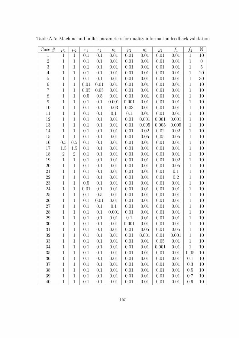
Table A.5: Machine and buffer parameters for quality information feedback validation
Case # µ1 µ2 r1 r2 p1 p2 g1 g2 f1 f2 N1 1 1 0.1 0.1 0.01 0.01 0.01 0.01 0.01 1 102 1 1 0.1 0.1 0.01 0.01 0.01 0.01 0.01 1 03 1 1 0.1 0.1 0.01 0.01 0.01 0.01 0.01 1 54 1 1 0.1 0.1 0.01 0.01 0.01 0.01 0.01 1 205 1 1 0.1 0.1 0.01 0.01 0.01 0.01 0.01 1 306 1 1 0.01 0.01 0.01 0.01 0.01 0.01 0.01 1 107 1 1 0.05 0.05 0.01 0.01 0.01 0.01 0.01 1 108 1 1 0.5 0.5 0.01 0.01 0.01 0.01 0.01 1 109 1 1 0.1 0.1 0.001 0.001 0.01 0.01 0.01 1 1010 1 1 0.1 0.1 0.03 0.03 0.01 0.01 0.01 1 1011 1 1 0.1 0.1 0.1 0.1 0.01 0.01 0.01 1 1012 1 1 0.1 0.1 0.01 0.01 0.001 0.001 0.001 1 1013 1 1 0.1 0.1 0.01 0.01 0.005 0.005 0.005 1 1014 1 1 0.1 0.1 0.01 0.01 0.02 0.02 0.02 1 1015 1 1 0.1 0.1 0.01 0.01 0.05 0.05 0.05 1 1016 0.5 0.5 0.1 0.1 0.01 0.01 0.01 0.01 0.01 1 1017 1.5 1.5 0.1 0.1 0.01 0.01 0.01 0.01 0.01 1 1018 2 2 0.1 0.1 0.01 0.01 0.01 0.01 0.01 1 1019 1 1 0.1 0.1 0.01 0.01 0.01 0.01 0.02 1 1020 1 1 0.1 0.1 0.01 0.01 0.01 0.01 0.05 1 1021 1 1 0.1 0.1 0.01 0.01 0.01 0.01 0.1 1 1022 1 1 0.1 0.1 0.01 0.01 0.01 0.01 0.2 1 1023 1 1 0.5 0.1 0.01 0.01 0.01 0.01 0.01 1 1024 1 1 0.01 0.1 0.01 0.01 0.01 0.01 0.01 1 1025 1 1 0.1 0.5 0.01 0.01 0.01 0.01 0.01 1 1026 1 1 0.1 0.01 0.01 0.01 0.01 0.01 0.01 1 1027 1 1 0.1 0.1 0.1 0.01 0.01 0.01 0.01 1 1028 1 1 0.1 0.1 0.001 0.01 0.01 0.01 0.01 1 1029 1 1 0.1 0.1 0.01 0.1 0.01 0.01 0.01 1 1030 1 1 0.1 0.1 0.01 0.001 0.01 0.01 0.01 1 1031 1 1 0.1 0.1 0.01 0.01 0.05 0.01 0.05 1 1032 1 1 0.1 0.1 0.01 0.01 0.001 0.01 0.001 1 1033 1 1 0.1 0.1 0.01 0.01 0.01 0.05 0.01 1 1034 1 1 0.1 0.1 0.01 0.01 0.01 0.001 0.01 1 1035 1 1 0.1 0.1 0.01 0.01 0.01 0.01 0.01 0.05 1036 1 1 0.1 0.1 0.01 0.01 0.01 0.01 0.01 0.1 1037 1 1 0.1 0.1 0.01 0.01 0.01 0.01 0.01 0.3 1038 1 1 0.1 0.1 0.01 0.01 0.01 0.01 0.01 0.5 1039 1 1 0.1 0.1 0.01 0.01 0.01 0.01 0.01 0.7 1040 1 1 0.1 0.1 0.01 0.01 0.01 0.01 0.01 0.9 10
155

Table A.6: Machine and buffer parameters for quality information feedback validation- continued
Case # µ1 µ2 r1 r2 p1 p2 g1 g2 f1 f2 N41 1.2 1 0.1 0.1 0.01 0.01 0.01 0.01 0.01 1 1042 1 1.2 0.1 0.1 0.01 0.01 0.01 0.01 0.01 1 1043 1.333 1 0.1 0.1 0.01 0.01 0.01 0.01 0.01 1 1044 1 1.333 0.1 0.1 0.01 0.01 0.01 0.01 0.01 1 1045 1.5 1 0.1 0.1 0.01 0.01 0.01 0.01 0.01 1 1046 1 1.5 0.1 0.1 0.01 0.01 0.01 0.01 0.01 1 1047 2 1 0.1 0.1 0.01 0.01 0.01 0.01 0.01 1 1048 1 2 0.1 0.1 0.01 0.01 0.01 0.01 0.01 1 1049 3 1 0.1 0.1 0.01 0.01 0.01 0.01 0.01 1 1050 1 3 0.1 0.1 0.01 0.01 0.01 0.01 0.01 1 10
156

Table A.7: Machine and buffer parameters for 3-state-machine and 2-state-machinecomparison ( Figures 5-5, 5-6, and 5-7)
Case # µ1 µ2 r1 r2 p1 p2 g1 g2 f1 f2 N QIF1 1.0 1.0 0.1 0.1 0.01 0.01 0.01 0.01 0.2 0.2 30 N2 1.0 1.0 0.1 0.1 0.01 0.01 0.01 0.01 0.2 0.2 5 N3 1.0 1.0 0.1 0.1 0.01 0.01 0.01 0.01 0.2 0.2 20 N4 1.0 1.0 0.1 0.1 0.01 0.01 0.01 0.01 0.2 0.2 50 N5 0.5 1.0 0.1 0.1 0.01 0.01 0.01 0.01 0.2 0.2 30 N6 2.0 1.0 0.1 0.1 0.01 0.01 0.01 0.01 0.2 0.2 30 N7 3.0 1.0 0.1 0.1 0.01 0.01 0.01 0.01 0.2 0.2 30 N8 1.0 1.0 0.01 0.01 0.01 0.01 0.01 0.01 0.2 0.2 30 N9 1.0 1.0 0.05 0.05 0.01 0.01 0.01 0.01 0.2 0.2 30 N10 1.0 1.0 0.5 0.5 0.01 0.01 0.01 0.01 0.2 0.2 30 N11 1.0 1.0 0.1 0.1 0.001 0.001 0.01 0.01 0.2 0.2 30 N12 1.0 1.0 0.1 0.1 0.05 0.05 0.01 0.01 0.2 0.2 30 N13 1.0 1.0 0.1 0.1 0.1 0.1 0.01 0.01 0.2 0.2 30 N14 1.0 1.0 0.1 0.1 0.01 0.01 0.001 0.001 0.2 0.2 30 N15 1.0 1.0 0.1 0.1 0.01 0.01 0.05 0.05 0.2 0.2 30 N16 1.0 1.0 0.1 0.1 0.01 0.01 0.1 0.1 0.2 0.2 30 N17 1.0 1.0 0.1 0.1 0.01 0.01 0.01 0.01 0.02 0.02 30 N18 1.0 1.0 0.1 0.1 0.01 0.01 0.01 0.01 0.5 0.5 30 N19 1.0 1.0 0.1 0.1 0.01 0.01 0.01 0.01 0.95 0.95 30 N20 1.0 1.0 0.5 0.1 0.01 0.01 0.01 0.01 0.2 0.2 30 N21 1.0 1.0 0.01 0.1 0.01 0.01 0.01 0.01 0.2 0.2 30 N22 1.0 1.0 0.1 0.5 0.01 0.01 0.01 0.01 0.2 0.2 30 N23 1.0 1.0 0.1 0.01 0.01 0.01 0.01 0.01 0.2 0.2 30 N24 1.0 1.0 0.1 0.1 0.1 0.01 0.01 0.01 0.2 0.2 30 N25 1.0 1.0 0.1 0.1 0.001 0.01 0.01 0.01 0.2 0.2 30 N26 1.0 1.0 0.1 0.1 0.01 0.1 0.01 0.01 0.2 0.2 30 N27 1.0 1.0 0.1 0.1 0.01 0.001 0.01 0.01 0.2 0.2 30 N28 1.0 1.0 0.1 0.1 0.01 0.01 0.1 0.01 0.2 0.2 30 N29 1.0 1.0 0.1 0.1 0.01 0.01 0.001 0.01 0.2 0.2 30 N30 1.0 1.0 0.1 0.1 0.01 0.01 0.01 0.1 0.2 0.2 30 N31 1.0 1.0 0.1 0.1 0.01 0.01 0.01 0.001 0.2 0.2 30 N32 1.0 1.0 0.1 0.1 0.01 0.01 0.01 0.01 0.9 0.2 30 N33 1.0 1.0 0.1 0.1 0.01 0.01 0.01 0.01 0.05 0.2 30 N34 1.0 1.0 0.1 0.1 0.01 0.01 0.01 0.01 0.2 0.9 30 N35 1.0 1.0 0.1 0.1 0.01 0.01 0.01 0.01 0.2 0.05 30 N36 1.0 1.0 0.1 0.1 0.01 0.01 0.01 0.01 0.2 0.2 5 N37 1.0 1.0 0.1 0.1 0.01 0.01 0.01 0.01 0.2 0.2 20 N38 1.0 1.0 0.1 0.1 0.01 0.01 0.01 0.01 0.2 0.2 50 N39 1.0 1.0 0.2 0.05 0.01 0.01 0.01 0.01 0.2 0.2 5 N40 1.0 1.0 0.2 0.05 0.01 0.01 0.01 0.01 0.2 0.2 20 N
157

Table A.8: Machine and buffer parameters for 3-state-machine and 2-state-machinecomparison ( Figures 5-5, 5-6, and 5-7)- continued
Case # µ1 µ2 r1 r2 p1 p2 g1 g2 f1 f2 N QIF41 1.0 1 0.2 0.05 0.01 0.01 0.01 0.01 0.2 0.2 50 N42 1.0 1 0.05 0.2 0.01 0.01 0.01 0.01 0.2 0.2 5 N43 1.0 1 0.05 0.2 0.01 0.01 0.01 0.01 0.2 0.2 20 N44 1.0 1 0.05 0.2 0.01 0.01 0.01 0.01 0.2 0.2 50 N45 1.0 1 0.1 0.1 0.01 0.01 0.01 0.01 0.2 0.2 30 N46 1.0 1 0.1 0.1 0.01 0.01 0.01 0.01 0.2 0.2 30 N47 1.0 1 0.1 0.1 0.01 0.01 0.01 0.01 0.2 0.2 30 N48 1.0 1 0.1 0.1 0.01 0.01 0.01 0.01 0.2 0.2 30 N49 1.0 1 0.1 0.1 0.01 0.01 0.01 0.01 0.2 0.2 30 N50 1.0 1 0.1 0.1 0.01 0.01 0.01 0.01 0.2 0.2 30 N51 1.2 1 0.1 0.1 0.01 0.01 0.01 0.01 0.2 0.2 30 N52 1.2 1 0.1 0.1 0.01 0.01 0.01 0.01 0.2 0.2 10 Y53 1.2 1 0.1 0.1 0.01 0.01 0.01 0.01 0.2 0.2 30 N54 1.2 1 0.1 0.2 0.02 0.01 0.01 0.005 0.2 0.2 30 N55 1.2 1 0.1 0.2 0.02 0.01 0.05 0.005 0.2 0.2 30 N56 1.33 1 0.1 0.1 0.01 0.01 0.01 0.01 0.2 0.2 30 N57 1.33 1 0.1 0.1 0.01 0.01 0.01 0.01 0.2 0.2 10 Y58 1.33 1 0.1 0.1 0.01 0.01 0.01 0.01 0.2 0.2 30 N59 1.33 1 0.1 0.2 0.02 0.01 0.03 0.01 0.3 0.1 30 N60 1.33 1 0.1 0.3 0.02 0.01 0.03 0.01 0.3 0.1 30 N61 1.50 1 0.1 0.1 0.01 0.01 0.01 0.01 0.2 0.2 30 N62 1.5 1 0.1 0.1 0.01 0.01 0.01 0.01 0.2 0.2 10 Y63 1.5 1 0.1 0.1 0.01 0.01 0.01 0.01 0.2 0.2 30 N64 1.5 1 0.1 0.4 0.05 0.01 0.01 0.01 0.2 0.2 30 N65 1.5 1 0.1 0.4 0.05 0.01 0.05 0.01 0.2 0.2 30 N66 2.0 1 0.1 0.1 0.01 0.01 0.01 0.01 0.2 0.2 30 N67 2.0 1 0.1 0.1 0.01 0.01 0.01 0.01 0.2 0.2 10 Y68 2.0 1 0.1 0.1 0.01 0.01 0.01 0.01 0.2 0.2 30 N69 2.0 1 0.08 0.3 0.05 0.01 0.05 0.008 0.4 0.2 30 N70 2.0 1 0.05 0.3 0.05 0.01 0.05 0.01 0.2 0.2 30 N71 3.0 1 0.1 0.1 0.01 0.01 0.01 0.01 0.2 0.2 30 N72 3.0 1 0.1 0.1 0.01 0.01 0.01 0.01 0.2 0.2 10 Y73 3.0 1 0.1 0.1 0.01 0.01 0.01 0.01 0.2 0.2 30 N74 3.0 1 0.08 0.18 0.2 0.015 0.01 0.01 0.1 0.2 30 N75 3.0 1 0.08 0.18 0.3 0.015 0.01 0.01 0.1 0.2 30 N76 1.0 1.2 0.1 0.1 0.01 0.01 0.01 0.01 0.2 0.2 30 N77 1.0 1.2 0.1 0.1 0.01 0.01 0.01 0.01 0.2 0.2 10 Y78 1.0 1.2 0.1 0.1 0.01 0.01 0.01 0.01 0.2 0.2 30 N79 1.0 1.2 0.2 0.1 0.01 0.02 0.005 0.01 0.2 0.2 30 N80 1.0 1.2 0.2 0.1 0.01 0.02 0.005 0.05 0.2 0.2 30 N
158
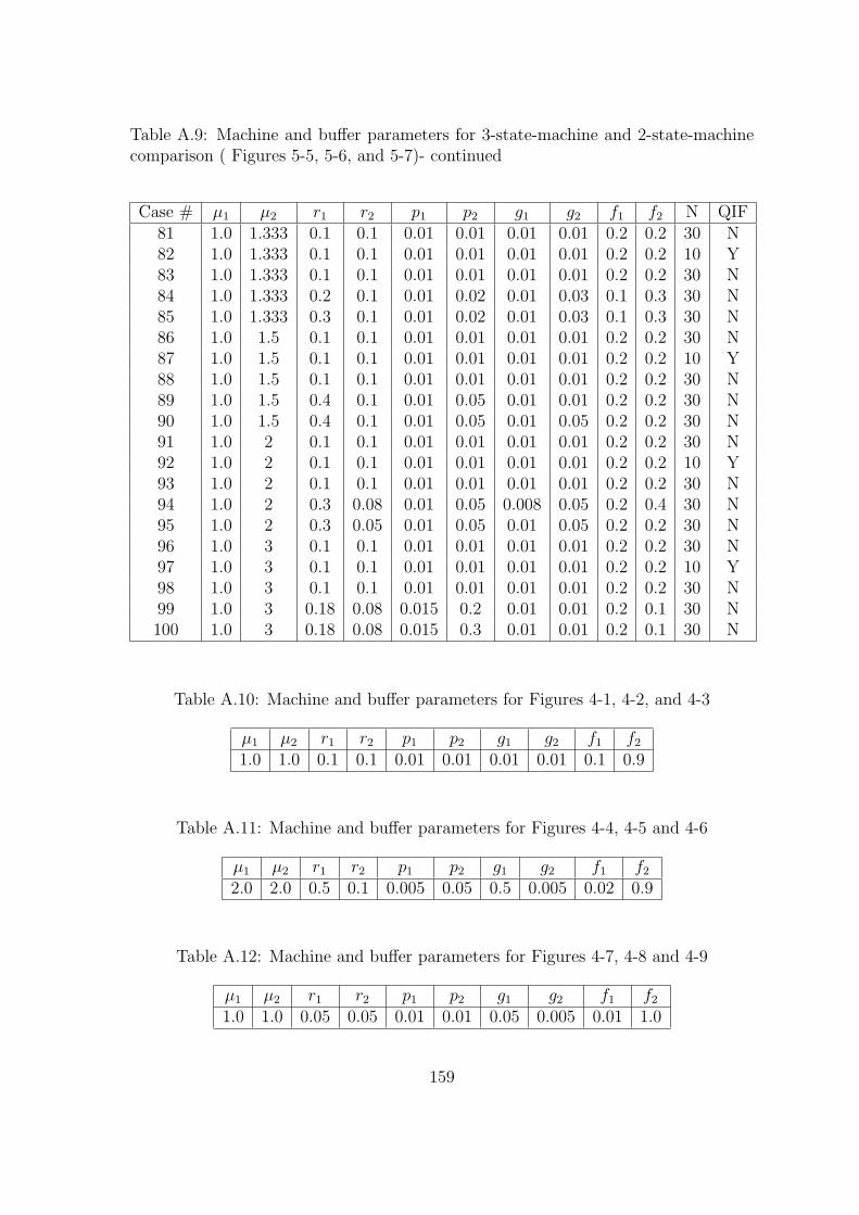
Table A.9: Machine and buffer parameters for 3-state-machine and 2-state-machinecomparison ( Figures 5-5, 5-6, and 5-7)- continued
Case # µ1 µ2 r1 r2 p1 p2 g1 g2 f1 f2 N QIF81 1.0 1.333 0.1 0.1 0.01 0.01 0.01 0.01 0.2 0.2 30 N82 1.0 1.333 0.1 0.1 0.01 0.01 0.01 0.01 0.2 0.2 10 Y83 1.0 1.333 0.1 0.1 0.01 0.01 0.01 0.01 0.2 0.2 30 N84 1.0 1.333 0.2 0.1 0.01 0.02 0.01 0.03 0.1 0.3 30 N85 1.0 1.333 0.3 0.1 0.01 0.02 0.01 0.03 0.1 0.3 30 N86 1.0 1.5 0.1 0.1 0.01 0.01 0.01 0.01 0.2 0.2 30 N87 1.0 1.5 0.1 0.1 0.01 0.01 0.01 0.01 0.2 0.2 10 Y88 1.0 1.5 0.1 0.1 0.01 0.01 0.01 0.01 0.2 0.2 30 N89 1.0 1.5 0.4 0.1 0.01 0.05 0.01 0.01 0.2 0.2 30 N90 1.0 1.5 0.4 0.1 0.01 0.05 0.01 0.05 0.2 0.2 30 N91 1.0 2 0.1 0.1 0.01 0.01 0.01 0.01 0.2 0.2 30 N92 1.0 2 0.1 0.1 0.01 0.01 0.01 0.01 0.2 0.2 10 Y93 1.0 2 0.1 0.1 0.01 0.01 0.01 0.01 0.2 0.2 30 N94 1.0 2 0.3 0.08 0.01 0.05 0.008 0.05 0.2 0.4 30 N95 1.0 2 0.3 0.05 0.01 0.05 0.01 0.05 0.2 0.2 30 N96 1.0 3 0.1 0.1 0.01 0.01 0.01 0.01 0.2 0.2 30 N97 1.0 3 0.1 0.1 0.01 0.01 0.01 0.01 0.2 0.2 10 Y98 1.0 3 0.1 0.1 0.01 0.01 0.01 0.01 0.2 0.2 30 N99 1.0 3 0.18 0.08 0.015 0.2 0.01 0.01 0.2 0.1 30 N100 1.0 3 0.18 0.08 0.015 0.3 0.01 0.01 0.2 0.1 30 N
Table A.10: Machine and buffer parameters for Figures 4-1, 4-2, and 4-3
µ1 µ2 r1 r2 p1 p2 g1 g2 f1 f2
1.0 1.0 0.1 0.1 0.01 0.01 0.01 0.01 0.1 0.9
Table A.11: Machine and buffer parameters for Figures 4-4, 4-5 and 4-6
µ1 µ2 r1 r2 p1 p2 g1 g2 f1 f2
2.0 2.0 0.5 0.1 0.005 0.05 0.5 0.005 0.02 0.9
Table A.12: Machine and buffer parameters for Figures 4-7, 4-8 and 4-9
µ1 µ2 r1 r2 p1 p2 g1 g2 f1 f2
1.0 1.0 0.05 0.05 0.01 0.01 0.05 0.005 0.01 1.0
159
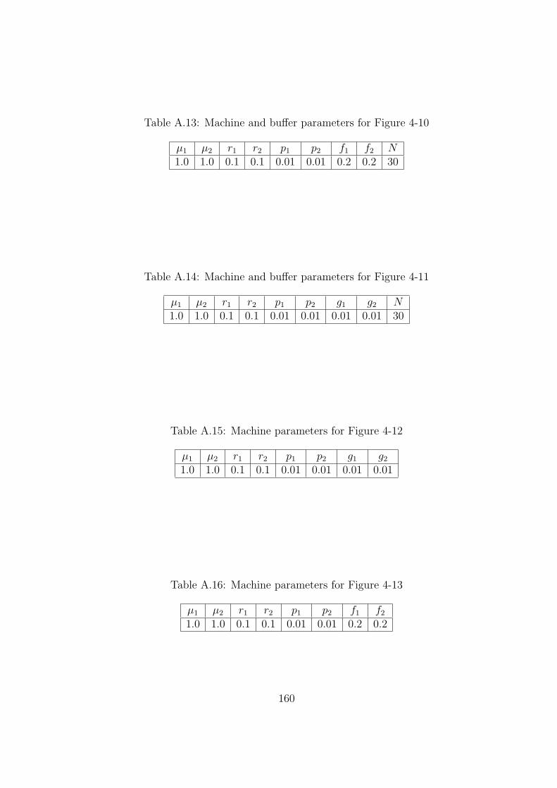
Table A.13: Machine and buffer parameters for Figure 4-10
µ1 µ2 r1 r2 p1 p2 f1 f2 N1.0 1.0 0.1 0.1 0.01 0.01 0.2 0.2 30
Table A.14: Machine and buffer parameters for Figure 4-11
µ1 µ2 r1 r2 p1 p2 g1 g2 N1.0 1.0 0.1 0.1 0.01 0.01 0.01 0.01 30
Table A.15: Machine parameters for Figure 4-12
µ1 µ2 r1 r2 p1 p2 g1 g2
1.0 1.0 0.1 0.1 0.01 0.01 0.01 0.01
Table A.16: Machine parameters for Figure 4-13
µ1 µ2 r1 r2 p1 p2 f1 f2
1.0 1.0 0.1 0.1 0.01 0.01 0.2 0.2
160
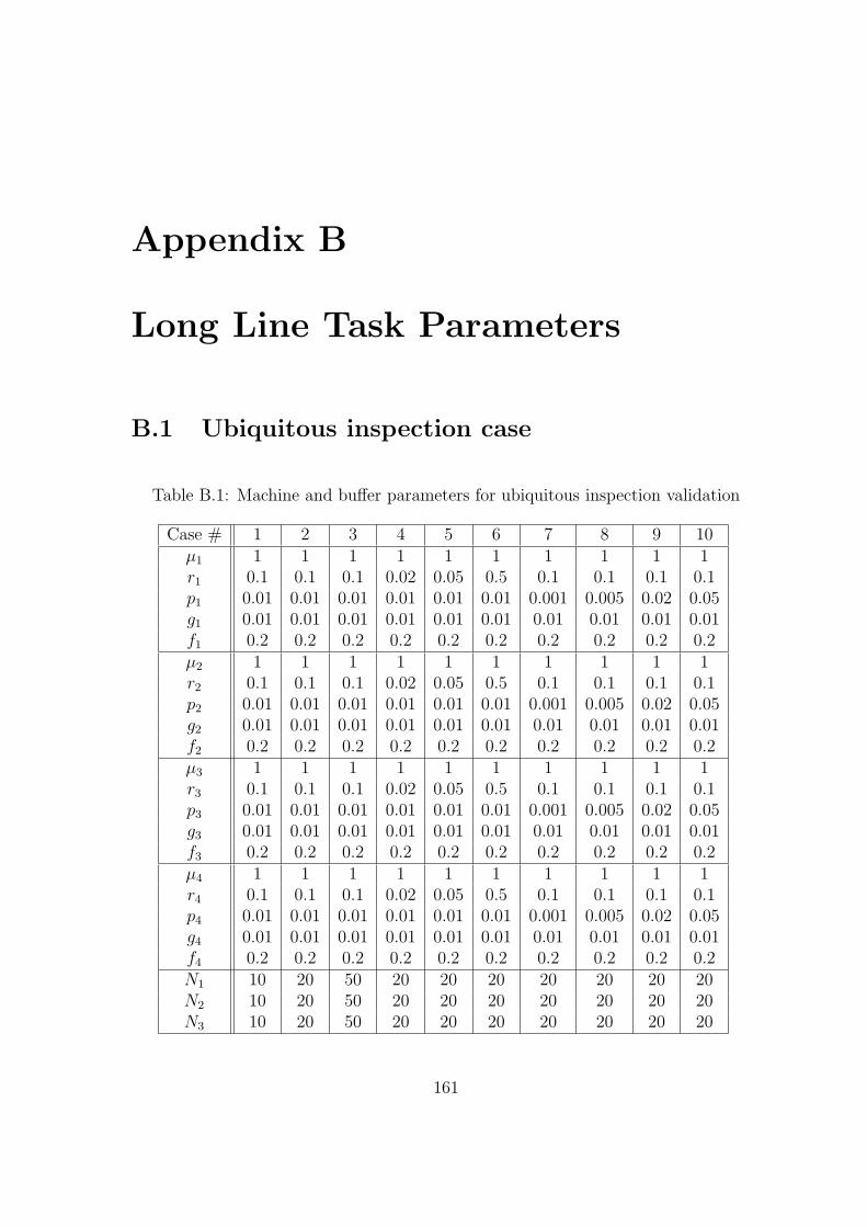
Appendix B
Long Line Task Parameters
B.1 Ubiquitous inspection case
Table B.1: Machine and buffer parameters for ubiquitous inspection validation
Case # 1 2 3 4 5 6 7 8 9 10µ1 1 1 1 1 1 1 1 1 1 1r1 0.1 0.1 0.1 0.02 0.05 0.5 0.1 0.1 0.1 0.1p1 0.01 0.01 0.01 0.01 0.01 0.01 0.001 0.005 0.02 0.05g1 0.01 0.01 0.01 0.01 0.01 0.01 0.01 0.01 0.01 0.01f1 0.2 0.2 0.2 0.2 0.2 0.2 0.2 0.2 0.2 0.2µ2 1 1 1 1 1 1 1 1 1 1r2 0.1 0.1 0.1 0.02 0.05 0.5 0.1 0.1 0.1 0.1p2 0.01 0.01 0.01 0.01 0.01 0.01 0.001 0.005 0.02 0.05g2 0.01 0.01 0.01 0.01 0.01 0.01 0.01 0.01 0.01 0.01f2 0.2 0.2 0.2 0.2 0.2 0.2 0.2 0.2 0.2 0.2µ3 1 1 1 1 1 1 1 1 1 1r3 0.1 0.1 0.1 0.02 0.05 0.5 0.1 0.1 0.1 0.1p3 0.01 0.01 0.01 0.01 0.01 0.01 0.001 0.005 0.02 0.05g3 0.01 0.01 0.01 0.01 0.01 0.01 0.01 0.01 0.01 0.01f3 0.2 0.2 0.2 0.2 0.2 0.2 0.2 0.2 0.2 0.2µ4 1 1 1 1 1 1 1 1 1 1r4 0.1 0.1 0.1 0.02 0.05 0.5 0.1 0.1 0.1 0.1p4 0.01 0.01 0.01 0.01 0.01 0.01 0.001 0.005 0.02 0.05g4 0.01 0.01 0.01 0.01 0.01 0.01 0.01 0.01 0.01 0.01f4 0.2 0.2 0.2 0.2 0.2 0.2 0.2 0.2 0.2 0.2N1 10 20 50 20 20 20 20 20 20 20N2 10 20 50 20 20 20 20 20 20 20N3 10 20 50 20 20 20 20 20 20 20
161

Table B.2: Machine and buffer parameters for ubiquitous inspection validation-continued
Case # 11 12 13 14 15 16 17 18 19 20µ1 1 1 1 1 1 1 1 1 0.5 1.5r1 0.1 0.1 0.1 0.1 0.1 0.1 0.1 0.1 0.1 0.1p1 0.01 0.01 0.01 0.01 0.01 0.01 0.01 0.01 0.01 0.01g1 0.001 0.005 0.02 0.05 0.01 0.01 0.01 0.01 0.01 0.01f1 0.2 0.2 0.2 0.2 0.02 0.05 0.5 0.9 0.2 0.2µ2 1 1 1 1 1 1 1 1 0.5 1.5r2 0.1 0.1 0.1 0.1 0.1 0.1 0.1 0.1 0.1 0.1p2 0.01 0.01 0.01 0.01 0.01 0.01 0.01 0.01 0.01 0.01g2 0.001 0.005 0.02 0.05 0.01 0.01 0.01 0.01 0.01 0.01f2 0.2 0.2 0.2 0.2 0.02 0.05 0.5 0.9 0.2 0.2µ3 1 1 1 1 1 1 1 1 0.5 1.5r3 0.1 0.1 0.1 0.1 0.1 0.1 0.1 0.1 0.1 0.1p3 0.01 0.01 0.01 0.01 0.01 0.01 0.01 0.01 0.01 0.01g3 0.001 0.005 0.02 0.05 0.01 0.01 0.01 0.01 0.01 0.01f3 0.2 0.2 0.2 0.2 0.02 0.05 0.5 0.9 0.2 0.2µ4 1 1 1 1 1 1 1 1 0.5 1.5r4 0.1 0.1 0.1 0.1 0.1 0.1 0.1 0.1 0.1 0.1p4 0.01 0.01 0.01 0.01 0.01 0.01 0.01 0.01 0.01 0.01g4 0.001 0.005 0.02 0.05 0.01 0.01 0.01 0.01 0.01 0.01f4 0.2 0.2 0.2 0.2 0.02 0.05 0.5 0.9 0.2 0.2N1 20 20 20 20 20 20 20 20 20 20N2 20 20 20 20 20 20 20 20 20 20N3 20 20 20 20 20 20 20 20 20 20
162

Table B.3: Machine and buffer parameters for ubiquitous inspection validation-continued
Case # 21 22 23 24 25 26 27 28 29 30µ1 2 1 1 1 1 1 1 1 1 1r1 0.1 0.3 0.1 0.1 0.1 0.1 0.1 0.1 0.1 0.1p1 0.01 0.01 0.01 0.01 0.01 0.05 0.01 0.01 0.01 0.01g1 0.01 0.01 0.01 0.01 0.01 0.01 0.01 0.01 0.01 0.05f1 0.2 0.2 0.2 0.2 0.2 0.2 0.2 0.2 0.2 0.2µ2 2 1 1 1 1 1 1 1 1 1r2 0.1 0.1 0.3 0.1 0.1 0.1 0.1 0.1 0.1 0.1p2 0.01 0.01 0.01 0.01 0.01 0.01 0.05 0.01 0.01 0.01g2 0.01 0.01 0.01 0.01 0.01 0.01 0.01 0.01 0.01 0.01f2 0.2 0.2 0.2 0.2 0.2 0.2 0.2 0.2 0.2 0.2µ3 2 1 1 1 1 1 1 1 1 1r3 0.1 0.1 0.1 0.3 0.1 0.1 0.1 0.1 0.1 0.1p3 0.01 0.01 0.01 0.01 0.01 0.01 0.01 0.05 0.01 0.01g3 0.01 0.01 0.01 0.01 0.01 0.01 0.01 0.01 0.01 0.01f3 0.2 0.2 0.2 0.2 0.2 0.2 0.2 0.2 0.2 0.2µ4 2 1 1 1 1 1 1 1 1 1r4 0.1 0.1 0.1 0.1 0.3 0.1 0.1 0.1 0.1 0.1p4 0.01 0.01 0.01 0.01 0.01 0.01 0.01 0.01 0.05 0.01g4 0.01 0.01 0.01 0.01 0.01 0.01 0.01 0.01 0.01 0.01f4 0.2 0.2 0.2 0.2 0.2 0.2 0.2 0.2 0.2 0.2N1 20 20 20 20 20 20 20 20 20 20N2 20 20 20 20 20 20 20 20 20 20N3 20 20 20 20 20 20 20 20 20 20
163
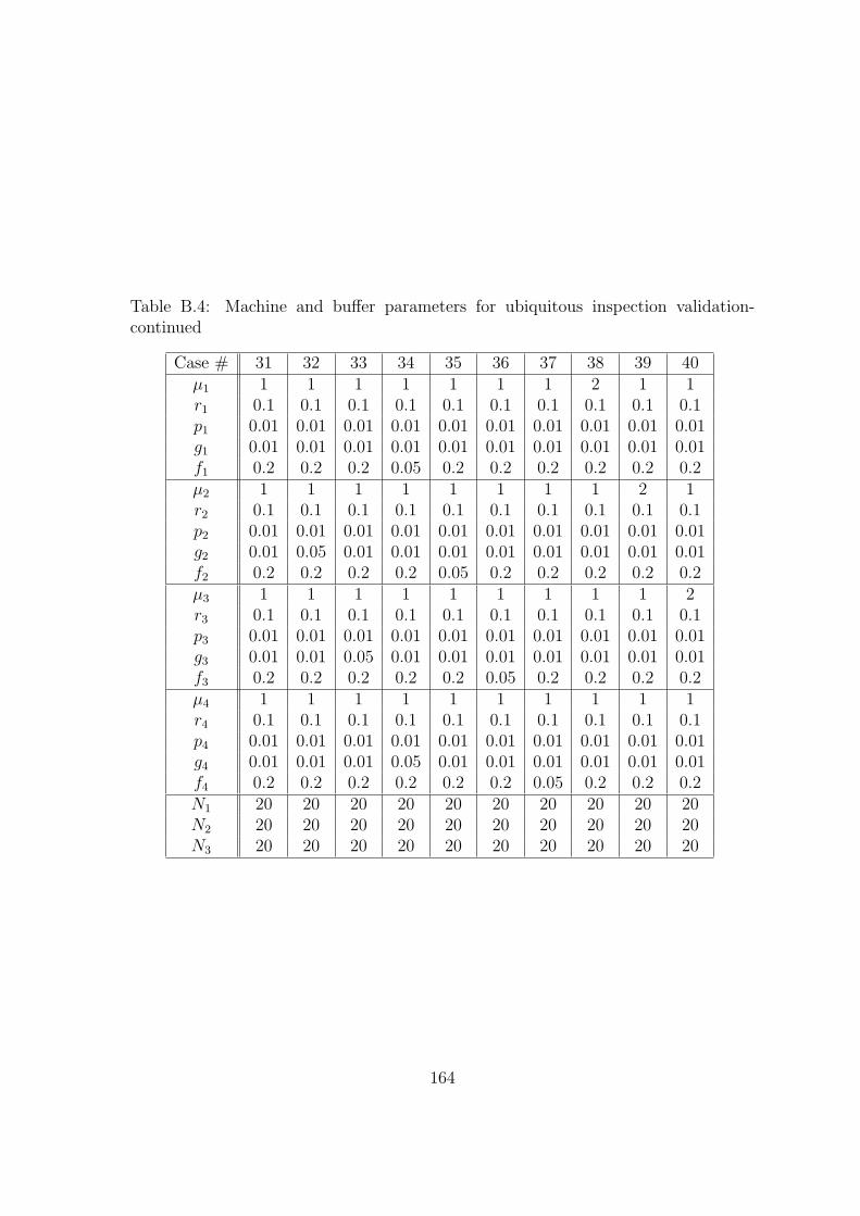
Table B.4: Machine and buffer parameters for ubiquitous inspection validation-continued
Case # 31 32 33 34 35 36 37 38 39 40µ1 1 1 1 1 1 1 1 2 1 1r1 0.1 0.1 0.1 0.1 0.1 0.1 0.1 0.1 0.1 0.1p1 0.01 0.01 0.01 0.01 0.01 0.01 0.01 0.01 0.01 0.01g1 0.01 0.01 0.01 0.01 0.01 0.01 0.01 0.01 0.01 0.01f1 0.2 0.2 0.2 0.05 0.2 0.2 0.2 0.2 0.2 0.2µ2 1 1 1 1 1 1 1 1 2 1r2 0.1 0.1 0.1 0.1 0.1 0.1 0.1 0.1 0.1 0.1p2 0.01 0.01 0.01 0.01 0.01 0.01 0.01 0.01 0.01 0.01g2 0.01 0.05 0.01 0.01 0.01 0.01 0.01 0.01 0.01 0.01f2 0.2 0.2 0.2 0.2 0.05 0.2 0.2 0.2 0.2 0.2µ3 1 1 1 1 1 1 1 1 1 2r3 0.1 0.1 0.1 0.1 0.1 0.1 0.1 0.1 0.1 0.1p3 0.01 0.01 0.01 0.01 0.01 0.01 0.01 0.01 0.01 0.01g3 0.01 0.01 0.05 0.01 0.01 0.01 0.01 0.01 0.01 0.01f3 0.2 0.2 0.2 0.2 0.2 0.05 0.2 0.2 0.2 0.2µ4 1 1 1 1 1 1 1 1 1 1r4 0.1 0.1 0.1 0.1 0.1 0.1 0.1 0.1 0.1 0.1p4 0.01 0.01 0.01 0.01 0.01 0.01 0.01 0.01 0.01 0.01g4 0.01 0.01 0.01 0.05 0.01 0.01 0.01 0.01 0.01 0.01f4 0.2 0.2 0.2 0.2 0.2 0.2 0.05 0.2 0.2 0.2N1 20 20 20 20 20 20 20 20 20 20N2 20 20 20 20 20 20 20 20 20 20N3 20 20 20 20 20 20 20 20 20 20
164
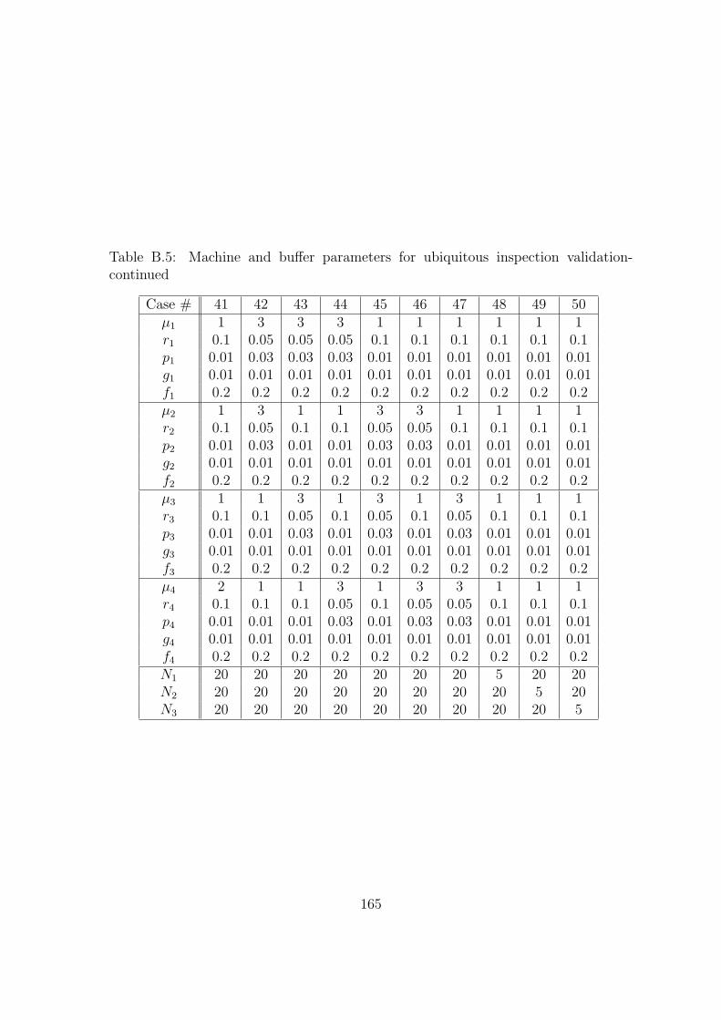
Table B.5: Machine and buffer parameters for ubiquitous inspection validation-continued
Case # 41 42 43 44 45 46 47 48 49 50µ1 1 3 3 3 1 1 1 1 1 1r1 0.1 0.05 0.05 0.05 0.1 0.1 0.1 0.1 0.1 0.1p1 0.01 0.03 0.03 0.03 0.01 0.01 0.01 0.01 0.01 0.01g1 0.01 0.01 0.01 0.01 0.01 0.01 0.01 0.01 0.01 0.01f1 0.2 0.2 0.2 0.2 0.2 0.2 0.2 0.2 0.2 0.2µ2 1 3 1 1 3 3 1 1 1 1r2 0.1 0.05 0.1 0.1 0.05 0.05 0.1 0.1 0.1 0.1p2 0.01 0.03 0.01 0.01 0.03 0.03 0.01 0.01 0.01 0.01g2 0.01 0.01 0.01 0.01 0.01 0.01 0.01 0.01 0.01 0.01f2 0.2 0.2 0.2 0.2 0.2 0.2 0.2 0.2 0.2 0.2µ3 1 1 3 1 3 1 3 1 1 1r3 0.1 0.1 0.05 0.1 0.05 0.1 0.05 0.1 0.1 0.1p3 0.01 0.01 0.03 0.01 0.03 0.01 0.03 0.01 0.01 0.01g3 0.01 0.01 0.01 0.01 0.01 0.01 0.01 0.01 0.01 0.01f3 0.2 0.2 0.2 0.2 0.2 0.2 0.2 0.2 0.2 0.2µ4 2 1 1 3 1 3 3 1 1 1r4 0.1 0.1 0.1 0.05 0.1 0.05 0.05 0.1 0.1 0.1p4 0.01 0.01 0.01 0.03 0.01 0.03 0.03 0.01 0.01 0.01g4 0.01 0.01 0.01 0.01 0.01 0.01 0.01 0.01 0.01 0.01f4 0.2 0.2 0.2 0.2 0.2 0.2 0.2 0.2 0.2 0.2N1 20 20 20 20 20 20 20 5 20 20N2 20 20 20 20 20 20 20 20 5 20N3 20 20 20 20 20 20 20 20 20 5
165

B.2 Extended quality information feedback case
Table B.6: Machine and buffer parameters for EQIF validation-continued
Case # 1 2 3 4 5 6 7 8 9 10µ1 1 1 1 1 1 1 1 1 1 1r1 0.1 0.1 0.1 0.1 0.1 0.1 0.1 0.1 0.1 0.1p1 0.01 0.01 0.01 0.05 0.05 0.05 0.002 0.002 0.002 0.01g1 0.01 0.01 0.01 0.002 0.002 0.002 0.05 0.05 0.05 0.01f1 0.01 0.01 0.01 0.05 0.05 0.05 0.002 0.002 0.002 0.01µ2 1 1 1 1 1 1 1 1 1 1r2 0.1 0.1 0.1 0.1 0.1 0.1 0.1 0.1 0.1 0.1p2 0.01 0.01 0.01 0.05 0.05 0.05 0.002 0.002 0.002 0.01g2 0 0 0 0 0 0 0 0 0 0f2 0.01 0.01 0.01 0.05 0.05 0.05 0.002 0.002 0.002 0.01µ3 1 1 1 1 1 1 1 1 1 1r3 0.1 0.1 0.1 0.1 0.1 0.1 0.1 0.1 0.1 0.1p3 0.01 0.01 0.01 0.05 0.05 0.05 0.002 0.002 0.002 0.01g3 0 0 0 0 0 0 0 0 0 0f3 0.01 0.01 0.01 0.05 0.05 0.05 0.002 0.002 0.002 0.01µ4 1 1 1 1 1 1 1 1 1 1r4 0.1 0.1 0.1 0.1 0.1 0.1 0.1 0.1 0.1 0.1p4 0.01 0.01 0.01 0.05 0.05 0.05 0.002 0.002 0.002 0.01g4 0 0 0 0 0 0 0 0 0 0f4 1 1 1 1 1 1 1 1 1 0.1N1 10 20 30 10 20 30 10 20 30 10N2 10 20 30 10 20 30 10 20 30 10N3 10 20 30 10 20 30 10 20 30 10
166

Table B.7: Machine and buffer parameters for EQIF validation-continued
Case # 11 12 13 14 15 16 17 18 19 20µ1 1 1 1 1 1 1 1 1 1 1r1 0.1 0.1 0.1 0.02 0.05 0.5 0.1 0.1 0.1 0.1p1 0.01 0.01 0.01 0.01 0.01 0.01 0.001 0.005 0.02 0.05g1 0.01 0.01 0.01 0.01 0.01 0.01 0.01 0.01 0.01 0.01f1 0.01 0.01 0.01 0.01 0.01 0.01 0.01 0.01 0.01 0.01µ2 1 1 1 1 1 1 1 1 1 1r2 0.1 0.1 0.1 0.02 0.05 0.5 0.1 0.1 0.1 0.1p2 0.01 0.01 0.01 0.01 0.01 0.01 0.001 0.005 0.02 0.05g2 0 0 0 0 0 0 0 0 0 0f2 0.01 0.01 0.01 0.01 0.01 0.01 0.01 0.01 0.01 0.01µ3 1 1 1 1 1 1 1 1 1 1r3 0.1 0.1 0.1 0.02 0.05 0.5 0.1 0.1 0.1 0.1p3 0.01 0.01 0.01 0.01 0.01 0.01 0.001 0.005 0.02 0.05g3 0 0 0 0 0 0 0 0 0 0f3 0.01 0.01 0.01 0.01 0.01 0.01 0.01 0.01 0.01 0.01µ4 1 1 1 1 1 1 1 1 1 1r4 0.1 0.1 0.1 0.02 0.05 0.5 0.1 0.1 0.1 0.1p4 0.01 0.01 0.01 0.01 0.01 0.01 0.001 0.005 0.02 0.05g4 0 0 0 0 0 0 0 0 0 0f4 0.5 0.1 0.5 1 1 1 1 1 1 1N1 10 20 20 20 20 20 20 20 20 20N2 10 20 20 20 20 20 20 20 20 20N3 10 20 20 20 20 20 20 20 20 20
167

Table B.8: Machine and buffer parameters for EQIF validation-continued
Case # 21 22 23 24 25 26 27 28 29 30µ1 1 1 1 1 1 1 1 1 1 1r1 0.1 0.1 0.1 0.1 0.1 0.1 0.1 0.1 0.1 0.1p1 0.01 0.01 0.01 0.01 0.01 0.01 0.01 0.01 0.01 0.01g1 0.001 0.005 0.02 0.05 0.01 0.01 0.01 0.01 0.01 0.01f1 0.01 0.01 0.01 0.01 0.01 0.01 0.01 0.01 0.01 0.01µ2 1 1 1 1 1 1 1 1 1 1r2 0.1 0.1 0.1 0.1 0.1 0.1 0.1 0.1 0.1 0.1p2 0.01 0.01 0.01 0.01 0.01 0.01 0.01 0.01 0.01 0.01g2 0 0 0 0 0 0 0 0 0 0f2 0.01 0.01 0.01 0.01 0.01 0.01 0.01 0.01 0.01 0.01µ3 1 1 1 1 1 1 1 1 1 1r3 0.1 0.1 0.1 0.1 0.1 0.1 0.1 0.1 0.1 0.1p3 0.01 0.01 0.01 0.01 0.01 0.01 0.01 0.01 0.01 0.01g3 0 0 0 0 0 0 0 0 0 0f3 0.01 0.01 0.01 0.01 0.01 0.01 0.01 0.01 0.01 0.01µ4 1 1 1 1 1 1 1 1 1 1r4 0.1 0.1 0.1 0.1 0.1 0.1 0.1 0.1 0.1 0.1p4 0.01 0.01 0.01 0.01 0.01 0.01 0.01 0.01 0.01 0.01g4 0 0 0 0 0 0 0 0 0 0f4 1 1 1 1 1 1 1 1 1 1N1 20 20 20 20 20 10 10 20 20 10N2 20 20 20 20 10 20 10 20 10 20N3 20 20 20 20 10 10 20 10 20 20
168

Table B.9: Machine and buffer parameters for EQIF validation-continued
Case # 31 32 33 34 35 36 37 38 39 40µ1 2 3 3 3 1 1 1 1 1 1r1 0.1 0.1 0.1 0.1 0.1 0.2 0.2 0.2 0.1 0.1p1 0.01 0.01 0.01 0.01 0.01 0.01 0.01 0.01 0.02 0.01g1 0.01 0.01 0.01 0.01 0.01 0.01 0.01 0.01 0.01 0.01f1 0.01 0.01 0.01 0.01 0.01 0.01 0.01 0.01 0.01 0.01µ2 3 2 3 3 1 1 1 1 1 1r2 0.1 0.1 0.1 0.1 0.2 0.1 0.2 0.2 0.1 0.1p2 0.01 0.01 0.01 0.01 0.01 0.01 0.01 0.01 0.01 0.02g2 0 0 0 0 0 0 0 0 0 0f2 0.01 0.01 0.01 0.01 0.01 0.01 0.01 0.01 0.01 0.01µ3 3 3 2 3 1 1 1 1 1 1r3 0.1 0.1 0.1 0.1 0.2 0.2 0.1 0.2 0.1 0.1p3 0.01 0.01 0.01 0.01 0.01 0.01 0.01 0.01 0.01 0.01g3 0 0 0 0 0 0 0 0 0 0f3 0.01 0.01 0.01 0.01 0.01 0.01 0.01 0.01 0.01 0.01µ4 3 3 3 2 1 1 1 1 1 1r4 0.1 0.1 0.1 0.1 0.2 0.2 0.2 0.1 0.1 0.1p4 0.01 0.01 0.01 0.01 0.01 0.01 0.01 0.01 0.01 0.01g4 0 0 0 0 0 0 0 0 0 0f4 1 1 1 1 1 1 1 1 1 1N1 20 20 20 20 20 20 20 20 20 20N2 20 20 20 20 20 20 20 20 20 20N3 20 20 20 20 20 20 20 20 20 20
169
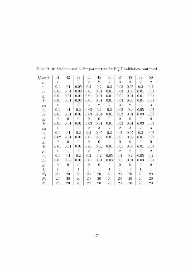
Table B.10: Machine and buffer parameters for EQIF validation-continued
Case # 41 42 43 44 45 46 47 48 49 50µ1 1 1 3 2 2 2 3 3 2 2r1 0.1 0.1 0.05 0.2 0.2 0.2 0.05 0.05 0.2 0.2p1 0.01 0.01 0.03 0.01 0.01 0.01 0.03 0.03 0.01 0.01g1 0.01 0.01 0.01 0.01 0.01 0.01 0.01 0.01 0.01 0.01f1 0.01 0.01 0.03 0.01 0.01 0.01 0.03 0.03 0.01 0.01µ2 1 1 2 3 2 2 3 2 3 3r2 0.1 0.1 0.2 0.05 0.2 0.2 0.05 0.2 0.05 0.05p2 0.01 0.01 0.01 0.03 0.01 0.01 0.03 0.01 0.03 0.03g2 0 0 0 0 0 0 0 0 0 0f2 0.01 0.01 0.01 0.03 0.01 0.01 0.03 0.01 0.03 0.03µ3 1 1 2 2 3 2 2 3 2 3r3 0.1 0.1 0.2 0.2 0.05 0.2 0.2 0.05 0.2 0.05p3 0.02 0.01 0.01 0.01 0.03 0.01 0.01 0.03 0.01 0.03g3 0 0 0 0 0 0 0 0 0 0f3 0.01 0.01 0.01 0.01 0.03 0.01 0.01 0.03 0.01 0.03µ4 1 1 2 2 2 3 2 2 3 2r4 0.1 0.1 0.2 0.2 0.2 0.05 0.2 0.2 0.05 0.2p4 0.01 0.02 0.01 0.01 0.01 0.03 0.01 0.01 0.03 0.01g4 0 0 0 0 0 0 0 0 0 0f4 1 1 1 1 1 1 1 1 1 1N1 20 20 20 20 20 20 20 20 20 20N2 20 20 20 20 20 20 20 20 20 20N3 20 20 20 20 20 20 20 20 20 20
170

B.3 Multiple quality information feedback case
Table B.11: Machine and buffer parameters for MQIF validation
Case # 1 2 3 4 5 6 7 8 9 10µ1 1 1 1 1 1 1 1 1 1 1r1 0.1 0.1 0.1 0.1 0.1 0.1 0.1 0.1 0.1 0.1p1 0.01 0.01 0.01 0.05 0.05 0.05 0.002 0.002 0.002 0.01g1 0.01 0.01 0.01 0.002 0.002 0.002 0.02 0.02 0.02 0.01f1 0.01 0.01 0.01 0.05 0.05 0.05 0.002 0.002 0.002 0.01µ2 1 1 1 1 1 1 1 1 1 1r2 0.1 0.1 0.1 0.1 0.1 0.1 0.1 0.1 0.1 0.1p2 0.01 0.01 0.01 0.05 0.05 0.05 0.002 0.002 0.002 0.01g2 0.01 0.01 0.01 0.002 0.002 0.002 0.02 0.02 0.02 0.01f2 0.01 0.01 0.01 0.05 0.05 0.05 0.002 0.002 0.002 0.01µ3 1 1 1 1 1 1 1 1 1 1r3 0.1 0.1 0.1 0.1 0.1 0.1 0.1 0.1 0.1 0.1p3 0.01 0.01 0.01 0.05 0.05 0.05 0.002 0.002 0.002 0.01g3 0.01 0.01 0.01 0.002 0.002 0.002 0.02 0.02 0.02 0.01f3 0.01 0.01 0.01 0.05 0.05 0.05 0.002 0.002 0.002 0.01µ4 1 1 1 1 1 1 1 1 1 1r4 0.1 0.1 0.1 0.1 0.1 0.1 0.1 0.1 0.1 0.1p4 0.01 0.01 0.01 0.05 0.05 0.05 0.002 0.002 0.002 0.01g4 0.01 0.01 0.01 0.002 0.002 0.002 0.02 0.02 0.02 0.01f4 1 1 1 1 1 1 1 1 1 0.1N1 10 20 30 10 20 30 5 10 15 10N2 10 20 30 10 20 30 5 10 15 10N3 10 20 30 10 20 30 5 10 15 10
171

Table B.12: Machine and buffer parameters for MQIF validation - continued
Case # 11 12 13 14 15 16 17 18 19 20µ1 1 1 1 1 1 1 1 1 1 1r1 0.1 0.1 0.1 0.02 0.05 0.5 0.1 0.1 0.1 0.1p1 0.01 0.01 0.01 0.01 0.01 0.01 0.001 0.005 0.02 0.05g1 0.01 0.01 0.01 0.01 0.01 0.01 0.01 0.01 0.01 0.01f1 0.01 0.01 0.01 0.01 0.01 0.01 0.01 0.01 0.01 0.01µ2 1 1 1 1 1 1 1 1 1 1r2 0.1 0.1 0.1 0.02 0.05 0.5 0.1 0.1 0.1 0.1p2 0.01 0.01 0.01 0.01 0.01 0.01 0.001 0.005 0.02 0.05g2 0.01 0.01 0.01 0.01 0.01 0.01 0.01 0.01 0.01 0.01f2 0.01 0.01 0.01 0.01 0.01 0.01 0.01 0.01 0.01 0.01µ3 1 1 1 1 1 1 1 1 1 1r3 0.1 0.1 0.1 0.02 0.05 0.5 0.1 0.1 0.1 0.1p3 0.01 0.01 0.01 0.01 0.01 0.01 0.001 0.005 0.02 0.05g3 0.01 0.01 0.01 0.01 0.01 0.01 0.01 0.01 0.01 0.01f3 0.01 0.01 0.01 0.01 0.01 0.01 0.01 0.01 0.01 0.01µ4 1 1 1 1 1 1 1 1 1 1r4 0.1 0.1 0.1 0.02 0.05 0.5 0.1 0.1 0.1 0.1p4 0.01 0.01 0.01 0.01 0.01 0.01 0.001 0.005 0.02 0.05g4 0.01 0.01 0.01 0.01 0.01 0.01 0.01 0.01 0.01 0.01f4 0.5 0.1 0.5 1 1 1 1 1 1 1N1 10 20 20 10 10 10 10 10 10 10N2 10 20 20 10 10 10 10 10 10 10N3 10 20 20 10 10 10 10 10 10 10
172

Table B.13: Machine and buffer parameters for MQIF validation - continued
Case # 21 22 23 24 25 26 27 28 29 30µ1 1 1 1 1 1 1 1 1 1 1r1 0.1 0.1 0.1 0.1 0.1 0.1 0.1 0.1 0.1 0.1p1 0.01 0.01 0.01 0.01 0.01 0.01 0.01 0.01 0.01 0.01g1 0.001 0.005 0.02 0.05 0.01 0.01 0.01 0.01 0.01 0.01f1 0.01 0.01 0.01 0.01 0.01 0.01 0.01 0.01 0.01 0.01µ2 1 1 1 1 1 1 1 1 1 1r2 0.1 0.1 0.1 0.1 0.1 0.1 0.1 0.1 0.1 0.1p2 0.01 0.01 0.01 0.01 0.01 0.01 0.01 0.01 0.01 0.01g2 0.001 0.005 0.02 0.05 0.01 0.01 0.01 0.01 0.01 0.01f2 0.01 0.01 0.01 0.01 0.01 0.01 0.01 0.01 0.01 0.01µ3 1 1 1 1 1 1 1 1 1 1r3 0.1 0.1 0.1 0.1 0.1 0.1 0.1 0.1 0.1 0.1p3 0.01 0.01 0.01 0.01 0.01 0.01 0.01 0.01 0.01 0.01g3 0.001 0.005 0.02 0.05 0.01 0.01 0.01 0.01 0.01 0.01f3 0.01 0.01 0.01 0.01 0.01 0.01 0.01 0.01 0.01 0.01µ4 1 1 1 1 1 1 1 1 1 1r4 0.1 0.1 0.1 0.1 0.1 0.1 0.1 0.1 0.1 0.1p4 0.01 0.005 0.01 0.01 0.01 0.01 0.01 0.01 0.01 0.01g4 0.001 0.01 0.02 0.05 0.01 0.01 0.01 0.01 0.01 0.01f4 1 1 1 1 1 1 1 1 1 1N1 10 10 10 10 20 10 10 20 20 10N2 10 10 10 10 10 20 10 20 10 20N3 10 10 10 10 10 10 20 10 20 20
173
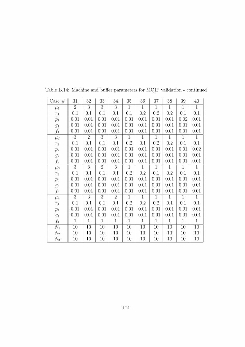
Table B.14: Machine and buffer parameters for MQIF validation - continued
Case # 31 32 33 34 35 36 37 38 39 40µ1 2 3 3 3 1 1 1 1 1 1r1 0.1 0.1 0.1 0.1 0.1 0.2 0.2 0.2 0.1 0.1p1 0.01 0.01 0.01 0.01 0.01 0.01 0.01 0.01 0.02 0.01g1 0.01 0.01 0.01 0.01 0.01 0.01 0.01 0.01 0.01 0.01f1 0.01 0.01 0.01 0.01 0.01 0.01 0.01 0.01 0.01 0.01µ2 3 2 3 3 1 1 1 1 1 1r2 0.1 0.1 0.1 0.1 0.2 0.1 0.2 0.2 0.1 0.1p2 0.01 0.01 0.01 0.01 0.01 0.01 0.01 0.01 0.01 0.02g2 0.01 0.01 0.01 0.01 0.01 0.01 0.01 0.01 0.01 0.01f2 0.01 0.01 0.01 0.01 0.01 0.01 0.01 0.01 0.01 0.01µ3 3 3 2 3 1 1 1 1 1 1r3 0.1 0.1 0.1 0.1 0.2 0.2 0.1 0.2 0.1 0.1p3 0.01 0.01 0.01 0.01 0.01 0.01 0.01 0.01 0.01 0.01g3 0.01 0.01 0.01 0.01 0.01 0.01 0.01 0.01 0.01 0.01f3 0.01 0.01 0.01 0.01 0.01 0.01 0.01 0.01 0.01 0.01µ4 3 3 3 2 1 1 1 1 1 1r4 0.1 0.1 0.1 0.1 0.2 0.2 0.2 0.1 0.1 0.1p4 0.01 0.01 0.01 0.01 0.01 0.01 0.01 0.01 0.01 0.01g4 0.01 0.01 0.01 0.01 0.01 0.01 0.01 0.01 0.01 0.01f4 1 1 1 1 1 1 1 1 1 1N1 10 10 10 10 10 10 10 10 10 10N2 10 10 10 10 10 10 10 10 10 10N3 10 10 10 10 10 10 10 10 10 10
174

Table B.15: Machine and buffer parameters for MQIF validation - continued
Case # 41 42 43 44 45 46 47 48 49 50µ1 1 1 3 2 2 2 3 3 2 2r1 0.1 0.1 0.05 0.2 0.2 0.2 0.05 0.05 0.2 0.2p1 0.01 0.01 0.03 0.01 0.01 0.01 0.03 0.03 0.01 0.01g1 0.01 0.01 0.01 0.01 0.01 0.01 0.01 0.01 0.01 0.01f1 0.01 0.01 0.03 0.01 0.01 0.01 0.03 0.03 0.01 0.01µ2 1 1 2 3 2 2 3 2 3 3r2 0.1 0.1 0.2 0.05 0.2 0.2 0.05 0.2 0.05 0.05p2 0.01 0.01 0.01 0.03 0.01 0.01 0.03 0.01 0.03 0.03g2 0.01 0.01 0.01 0.01 0.01 0.01 0.01 0.01 0.01 0.01f2 0.01 0.01 0.01 0.03 0.01 0.01 0.03 0.01 0.03 0.03µ3 1 1 2 2 3 2 2 3 2 3r3 0.1 0.1 0.2 0.2 0.05 0.2 0.2 0.05 0.2 0.05p3 0.02 0.01 0.01 0.01 0.03 0.01 0.01 0.03 0.01 0.03g3 0.01 0.01 0.01 0.01 0.01 0.01 0.01 0.01 0.01 0.01f3 0.01 0.01 0.01 0.01 0.03 0.01 0.01 0.03 0.01 0.03µ4 1 1 2 2 2 3 2 2 3 2r4 0.1 0.1 0.2 0.2 0.2 0.05 0.2 0.2 0.05 0.2p4 0.01 0.02 0.01 0.01 0.01 0.03 0.01 0.01 0.03 0.01g4 0.01 0.01 0.01 0.01 0.01 0.01 0.01 0.01 0.01 0.01f4 1 1 1 1 1 1 1 1 1 1N1 10 10 10 10 10 10 10 10 10 10N2 10 10 10 10 10 10 10 10 10 10N3 10 10 10 10 10 10 10 10 10 10
175

176

Appendix C
Matrix manipulation technique
Matrix A in equations (3.165), (3.166), and (3.167) contains elements which can be
different by several orders of magnitude (e.g., eλiNZji Y
ji and Y j
i ). When λ > 0 and
N is large, this may cause the reduction of the apparent rank of matrix A, which
will lead to errors. To prevent this, following technique is used for solving equations
(3.165), (3.166), and (3.167).
• Build a new matrix A′ by doing:
– For each column i in matrix A, check if the column contains eλiN .
– For the column that contains eλiN terms, divide all the elements in the
column by eλiN if λi > 0.
• Calculate X ′ which is a solution of A′X ′ = B using numerical methods.
• Divide the elements in X ′ by eλiN if corresponding column in A is modified.
This gives X which is the solution of the original equation AX = B.
177
Top Related