


Languages
Pages
Legal


RD-RI50 ?36 MODELING AND CONTROL OF LARGE FLEXIBLE STRUCTURES(U) 1/2SYSTEMS ENGINEERING FOR POWER INC ANNANDALE VA8 RYRAMOVIC ET AL. 31 JUL 84 SEPI-TR-84-9
EIEIIIR0IIIIIIIIIIIIIIIIII..fflfIEEEEEIIIIIIIIIIIIIIIIIIIIIlI I I IIIllll lfll

L 28 fl
:16
NtOA.BEAO SARS93MICROCOPY RESOLUTION TEST CHART '-.,
%.1.3%
UFOSR. 85-0075
*YWIMU ENMNEMNO FOR PO01, INCANNANOAL- VININ ° A
MODELING AND CONTROL OF LARGE FLEXIBLE STRUCTURES
Final Report on Phase I Research
Contract No. F49620-83-C-0l59
AFOSR/NADirectorate of Aerospace Sciences
Building 410Bolling APB
Washington, D.C. 20332
ATTN: Dr. A. Amos
July 31, 1984 DTICELECTEFEB 2 8 85
B
Bpproved f or pub1"- r-:".1.dis.tribut ionunliltode
85 02 13 052 ."0
- ~.... .............._.. ~............ ,.............,.....,,,.,,,......•.,.....--. ,...,-..-..

-...- *. - -. . . .. . --,-.,.--,--.- -
'E*RT CLASSIFICATICON OF THISPAEroDaenled6p
READ INSTRUCTIONSREPOT DOCUMENTATION PAGE BEFORE COMPLETING FORMQEPOR- NUJMBER 2. GOVT ACCESSION NO. 3. RECIPIENT'S CATALOG NUMBERAFSsR o - ,- '-' L4 >-lSo'.3 ..-
4. T IY L E(dindS. TYPE OF REPORT I PERIOD COVERED
Modeling and Control of Large Flexible Structures p ,a9Sept. 30, 1982-may 31. 1984-6. PERFORMING ORG. REPORT NUMBER
SEPI TR 84-97- AT OR &)S. CONTRACT OR GRANT NuMBER(s)B. Avramovic
B.avrk=zkai G.L. Blanken shipN. B a. KwatniF4962C-83-C-0:59
< ennt t L-""". _
P A 41ZW'C ;:4E AN D A r:R ES 5- 'C. PRC-RAME .E-EN-T.PROJEC T, ASKAREA W *rK UNT NCu8ERS
an e, S Uite 3., an VA 0 -
~11 C N7RAL!.ANG O,#FiCE -iAM~E AND ADCRESS $. FPCT ZATE
, L 7 -Z3 N-N5ER OF FACES k
74. U, NITORING AGENCYNAME A ADORESS - ii f dltfeng frog, Conr,ollng Off;ce) 15. SEC .RJTY C LASS. (of uf. ,Uh~a ) -p "
Unclassified15.. - tAiSF- CA ;N ;W.R A NG
SCEDULE
06. OSIT R SuTICN STAT EmENT (of A. eport)
Approved for public release; distribution unlimited.
!7. O;STR, SUT)ON STATEMENT (of t.' a .a: fv: f.,.d ,. S'.,cA 2Vi. 0, I rer? itoe erpo Reprt)
I6. StPPLEMENTARY NOTES
K iY WORDS (Co&n. on :e*e i.)neand Identify by b~ockn-b,
ACTIVE CONTROLS/ HOMOGENI ZATION.VIBRATION CONTROL, LATTICE STRUCTURE,DISTRIBUTED FEEDBACK CONTROL, PERIODICITY-SPECTRAL METHODS, <-
20. A S RACT' {' t re-e *i If .d Iden2,iy by bock nmbiw)
The main emphasis in the first phase of this work has been theadaptation and enhancement of certain Wiener-Hopf methods for control systemdesign used by J. Davis for the treatment of linear, dynamic, distributed
Iameter mde---o. -- Iiexible structur Davis developed a frequency domain.... .hodology_ for computing k=l=: -uula rgnht- febc ~ isrqecfrdmi_..i r, a 'sgu atcr fedbacr e ,-ns f r ifnearpotribused Wiener-Hopf spectral factorza~ion.
he numercal algforithms for executin-g the spectral factorization were asedon somae r'i- work of . Sten'er. -* r cas-4d
%..W~ 147 EDITIONO orINOV 6 S BSSOLETE UCA~FE
SECLR#Ty CL ASSIFI&77C l -4 ,F 'rmIS PA.E , Z-' E.. e )
,.F.
SECURITY CLASSIFICATION Or THIS PAGE(Wa DWI Ej lt . , p.
.
The Davis-Stenger methodology was adapted to the problem ofvibration control of flexible structures. The spectral factorizationmethodology avoids the difficult numerical problems associated with .the solution of the Riccati partial differential equations which arise4n the time domain approach for designing stabilizing controllers. Inthis way distributed phenomena, like travelling waves, whichcharacterize the macroscopic dy-namics of flexible structures areretained in the model, and their interaction with the control system
,. preserved :he analyt:cal design rr:cess. :omrutational.algor tnms were developed and several :rotot pe systems were treatedincluding the Euer Beam and a simple two dimersional system.
Second part of the research involved t1e use of a mathematicaltechnioue for asymptotic analysis called -omogenization. aoriginaiiydeveloped by I. Babuska, to produce simplified models for flexiblestructures with a regular (periodic) infrastructure. "omogenizationcf the model for a structure with a regulr infrastructure produces amodel with smoothly varying effective parameters for mass density,local tenc@ion, and damping that represents a flexible structure withu nif o r m ~hmg eiZe n t e r na st r u ct u re. . 4
The homogenization technique does not require the a prioriassumption of a specific continuum structure as the approximation fora given lattice structure. Instead, the asymptotic analysis of theoriginal structure produces the distributed continuum approximationmc~el of the lattice s:ructure in the :imt as some characteristic
m (e.g., inter-cell dimension in the structural model goes tozero. Moreover, the natural averaging process is developed in thecourse of the analsis. It is r.asy to construct examples in which the:rocedure of averaging :.arameters over a c"--racteristic volume leadsto incorrect approximations for thr system d-nami cs. Thehomogenization methods used in this re. earch are based on theassumption of a periodic infrastructure in the original model. Thisis not necessary, and random structures can also be treated, if therandomness has sufficient ergodicity properties (in the spatialvariables).
:omogenization and asymptotic analysis can also be carried out inthe context of control and state estimation problems for heterogeneousstructures. It is important that the control and homogenizationprocedure not be done separately, since one can construct examples inwhich control designs based on averaged models are not correct asapproximations to the optimal (e.g., regulator) control laws for theoriginal problem. While control and filtering theory withhomogenization is not very advanced at this stage, prototype problemscan be analyzed to a point where the basic features of design % :-algorithms are clear.
'C, C LA S SI JZ7 ED
SECI,. CLASSIFICAT,^ N F -, 4?.r, Z.:a £ ee'd
MODELING AND CONTROL OF LARGE FLEXIBLE STRUCTURES
Final Report on Phase I Research
Contract No: 149620-83-C-0159
APOSR/NADirectorate of Aerospace Sciences
Building 410Boiling APB
Washington, DC 20332
ATTN: Dr. A. Amos
31 July 19S4
C Submitted by: Prepared by:
SEPI B. AvramovicSuite 302 N. Barkakati
* ' 4300 Evergreen Lane W. BennettAnnandale, VA 22003 G.L. Blankenship(703)-941-6206 H.G. Kwatny
Approved for public release; Distribution unlimited
The views and conclusions contained in this report are those of theauthors and should not be interpreted as necessarily representing theofficial policies or endorsements, either expressed or implied, of theAir Force Office of Scientific Research or the U.S. Government.
'... AIR FORCE 07 ,?1 ,!TNT"YTC RCI kR) (A(..y),, l0TI CS OF TRP4'T TT .I" L D"T..
". . .' ~~This tethnr,: '- .- ' -, .d and is
Distribution i3 ualimitfd.MATTHEW J. X3WChief, Teshnical Informat o Division
"" -c,. . , -q .. .,-r .-. "+ q .q- .- t ,W% % , - . tV ... . % . . %- -% +,,%, ,, -. . .. .

CONTENTS
List of Figures
Summary of Phase I Research
Part I. Wiener-Kopf Methods for Control System Design
1. Background: Dynamical control of flexible 111tue
*1.1 Generic models of the dynamics of flexible structures 31.2 State space models and modal control 51.*3 Control of a vibrating flexible string 81.4 Control of a two-dimensional hyperbolic system 10
%1.5 Control of a simply supported beam 14
2. Wiener-Kopf Methods for Control System Design:The Davis-Stenger Algorithm 16
2.1 Davis's method 192.2 Stenger's algorithm for spectral factorization 25
3. Control of a One-Dimensional Structure 30
3.1 Control of a flexible beam 30
S3.2 Numerical results 34
4. Control of a Two-dimensional Prototype System 44
4.1 Dynamics of a vibrating membrane 454.2 Transfer function of the controlled membrane 524.3 Solution of the elliptic system using the
discretized Green's function 564.4 Nigenfunction expansion of the solution of the
generalized wave equation 594.5 Spectral factorization using the Hilbert transform 624.6 Gain computations 644.7 Software development and control system performance 66
Part II. Effective Parameter Models of Heterogeneous Structures
5. Homogenization of Regular Structures 70
5.1 A one-dimensional example 735.2 Homogenization of wave equations 755.3 Continuum approximations for lattice structures 80
5.3.1 Effective conductivity of a periodic lattice 81L5.3.2 Continuum model for motions of a truss element 91
6. Homogenization and Optimal Stochastic Control 102
-* T
%, **
- 6.1 A prototype problem 1026.2 Hamilton - Jacobi equation 1066.3 Identification and interpretation of the limit
problem 108
- 6.4 Application: Homogenization-optimization of lattice
7. Homogenization and State Estimation in HeterogenousP Structures 117
7.1 Problem statement and background 1177.2 Preliminary analysis 1177.3 The filtering problem 1257.4 A duality form and an expression for the conditional
density 1277.5 Homogenization 133
8. Open Problems and Further Work 142
References 147
Appendix A: Experimental Results for the Euler Beam Al
• .9
.9 .° -
Accession For
NTIS GPA*&IDTIC TAB E"Unannounced 0
DTIC%°.,* ,..'.°
copyIN4SPECTED By
Distribution/ '
.9 Availability Codes"Aval.l and/or
Dist Speclal-
d" .- '-
-e *., ° '.- ' '* .*
.p.,
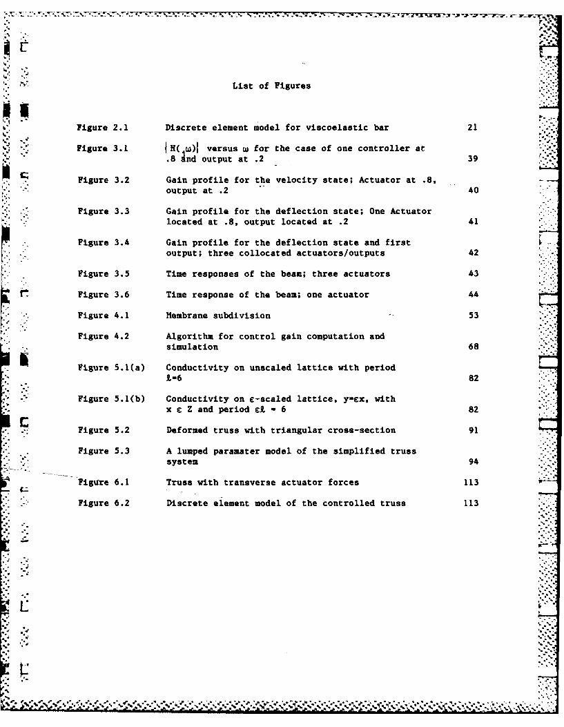
List of Figures
Figure 2.1 Discrete element model for viscoelastic bar 21
S'Figure 3.1 1H( w)1 versus w for the case of one controller at.8 Ind output at .2 39
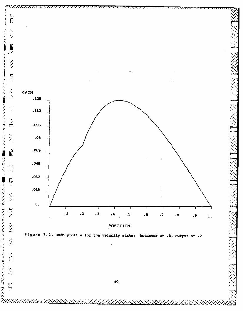
Figure 3.2 Gain profile for the velocity state; Actuator at .8,output at .2 40
Figure 3.3 Gain profile for the deflection state; One Actuatorlocated at .8, output located at .2 41
- Figure 3.4 Gain profile for the deflection state and firstoutput; three collocated actuators/outputs 42
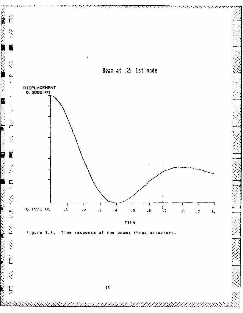
Figure 3.5 Time responses of the beam; three actuators 43
Figure 3.6 Time response of the beam; one actuator 44
-" Figure 4.1 Membrane subdivision 53
" Figure 4.2 Algorithm for control gain computation andsimulation 68
Figure 5.1(a) Conductivity on unscaled lattice with period
--6 82
Figure 5.1(b) Conductivity on c-scaled lattice, y-ex, withx c Z and period et - 6 82
. Figure 5.2 Deformed truss with triangular cross-section 91
Figure 5.3 A lumped paramater model of the simplified truss
system 94
Figure 6.1 Truss with transverse actuator forces 113
" Figure 6.2 Discrete element model of the controlled truss 113
.- ,'= -
.- . :. .,-:
?%, . . . V V *'* *. . . ...- '*....-....-,
. .
Summary of Phase I Research
Interaction of the control system with the structural dynamics ofthe physical system is one of the fundamental issues in large spacestructure applications. Our work is intended to contribute directly
* -. to understanding this interaction by using models which capture the
E7 essential distributed character of the system, and using analyticaltechniques vhich preserve the character of the physical system in themodel simplification process. The methods we have used -
Wiener-Hopf/spectml factorization methods for design of distributedcontrol systems and homogenization/asymptotic analysis for modelsimplification -- have tremendous potential for the analyticaltreatment of complex structural control problems, including thesyanthesis of computer-aided-design methods for large spacestructures. In Phase I of this project, we have concentrated on thetreatment of a few simple prototype systems. Further work is neededto adapt and enhance the methods to treat complex structures. Theanalytical methods themselves do not require substantial extensions.Rather, their potential for the treatment of complex flexiblestructures should be developed.
The main emphasis in the first phase of this work has been the* -adaptation and enhancement of certain Wiener-Kopf methods for control
system design used by J. Davis for the treatment of linear, dynamic,distributed parameter models of flexible structures. Davis developeda frequency domain methodology for computing optimal (regulator)feedback gains for linear distributed parameter control systems by
-: ~ Wiener-Hopf spectral factorization. The numerical algorithms forexecuting the spectral factorization were based on some earlier work
* of F. Stenger. We have adapted the Davis-Stenger methodology to theproblem of vibration control of flexible structures. A generic
* problem of this type is the figure control of a large space antenna.We have carried out the analysis and computed the optimal feedbackregulator control laws for several examples including theEuler-Bernoulli beam model and a two-dimensional prototype(experimental) system studied by J. Lang and D. Staelin.
~ This portion of the research has demonstrated the effectivenessof frequency domain -- spectral factorization methods for the designof control and state estimation algorithms for flexible structuresdescribed by linear distributed parameter models (hyperbolic partialdifferential equations). In this approach it is not necessary toreduce the models to finite dimensional (lumped parameter) models at
Lthe outset of the design procedure. The infinite dimensionalcharacter of the system is preserved throughout the design process.The spectral factorization methodology avoids the difficult numerical
*problems associated with the solution of the Riccati partialdifferential equations which arise in the time domain approach fordesigning stabilizing controllers. In this way distributed phenomena,
% like travelling waves, which characterize the macroscopic dynamics offlexible structures are retained in the model, and their interactionwith the control system is preserved in the analytical design process.
II o '-.4

%. .0
In the second part of the research ws have examined the use of amathematical technique for asymptotic analysis called"homogenization", originally developed by I.* Babuska, to producesimplified models for flexible structures with a regular (periodic)infrastructure. Homogenization of the model for a structure with aregular infrastructure produces a model with smoothly varying"effective" parameters for mass density, local tension, and dampingthat represents a flexible structure with a uniform "homogenized"internal structure. The derivation of continuum models for complexstructures with a regular infrastructure has been studied for manyyears in applied mechanics. In most cases the continuum models arebased on local averages of the physical parameters (e.g., massdensity, stress, strain, etc.) over some characteristic volume of thestructure. The averaged quantities computed in this way are relatedto the associated quantities in a postulated continuum structure. Forexample, the mass density and stress tensors in a long truss with aregular lattice structure have been related to the distributedparameters in a beam (in the work of Noor, Nayfeh, and Renton, amongothers).
Our technique does not require the a priori assumption of aspecific continuum structure as the approximation for a given latticestructure. Instead, the asymptotic analysis of the original structureproduces the distributed continuum rpproximation model of the latticestructure in the limit as some characteristic parameter (e.g.,inter-cell dimension) in the structural model goes to zero. Moreover,the natural averaging process is developed in the course of theanalysis. It is easy to construct examples in which the usualprocedure of averaging parameters over a characteristic volume leadsto incorrect approximations for the system dynamics. Thehomogenization methods used in our research are based on theassumption of a periodic infrastructure in the original model. Thisis not necessary, and random structures can also be treated, if the
0~ randomness has sufficient ergodicity properties (in the spatialvariables). Numerical evaluations of the averaged model are more
* difficult in this case.
Homogenization and asymptotic analysis can also be carried out inthe context of control and state estimation problems for heterogeneousstructures. It is important that the control and homogenizationprocedure not be done separately, since one can construct examples inwhich control designs based on averaged models are not correct as 1approximations to the optimal (e.g., regulator) control laws for theoriginal problem. While control and filtering theory with r7homogenization is not very advanced at this stage, it is neverthelesspossible to analyze some prototype problems to a point where the basic
*0 features of the theory are clear. Our work has contributed to thisprocess, but much more needs to be done.
el
.It
;,, "..-
,. ,-,,o',, .4.
: ") Part I: :i:
'i" '" Wierner-Hopf Methods for Design of Stabilizing Control Systems ::
Z'" ..-- -~
. . . . .. . . . . . . ... . . . . .......- ~ ... . S 5 * * .5 .. ** .*% - * 5*55 * . . . . % % ' * . ' % , . :.:.

-A-- - .. o°-.'- --- "
1. Background: Dynamical Control of Flexible Structures
Interaction of the control system with the structural dynamics of
the mechanical system is one of the fundamental issues in large space .- '-
structure applications. Our work is intended to contribute directly
to understanding this interaction by using models which capture the
essential distributed character of the system, and using analytical
techniques which preserve the character of the physical system in the
model simplification process. The methods we have used --
Wiener-Hopf/spectral factorization methods for design of distributed
control systems and homogenization/asymptotic analysis for model .- ,
simplification -- have tremendous potential for the analytical
treatment of complex structural control problems, including the
synthesis of computer-aided-design methods for large space structures.
In Phase I of this project, we have concentrated on the treatment of a
few simple prototype systems. The methods may be adapted to treat
complex structures. They do not require substantial extensions for
such cases. Rather, computational algorithms which translate their
strengths into effective design tools need to be developed.
The main emphasis in the first part of this work has been the
adaptation and enhancement of certain Wiener-Hopf methods for control
system design used by J. Davis for the treatment of linear, dynamic,
distributed parameter models of flexible structures (Davis 1978, ,
1979a,b 1982) (Davis and Barry 1977) (Davis and Dickenson 1983).
Davis and his colleagues developed a frequency domain methodology for
computing optimal (regulator) feedback gains for linear distributed
parameter control systems by Wiener-Hopf spectral factorization. The
1
.. . . . .. •.; ,-.,-. , ,.,'.r-, / ..... .. . ;; ./ . ',.'.. ,.','..'./,/.. -'.,. ,..% .. , ...
numerical algorithms for executing the spectral factorization vere
based on some earlier work of F. Stenger (1972). We have adapted the
Davis-Stenger methodology to the problem of vibration control of
C_ flexible structures. A generic problem of this type is the figure
control of a large space antenna. We have carried out the analysis
- and computed the optimal feedback regulator control laws for several
examples including the Euler-beam. and a two-dimensional prototype
(experimental) system studied by J. Lang and D. Staelin (Lang and
Staelin 1982a,b).
This portion of the research has demonstrated the effectiveness
of frequency domain -- spectral factorization methods for the design
of control and state estimation algorithms for flexible structures
I described by linear distributed parameter models (hyperbolic partial
* . differential equations). In this approach it is not necessary to
reduce the models to finite dimenaional (lumped parameter) models at
the outset of the design procedure. The infinite dimensional
character of the system is preserved throughout. The spectral
- factorization methodology avoids the difficult numerical problems
associated with the solution of the Riccati partial differential
equations which arise in the time domain approach for designing
ftstabilizing controllers. In this way distributed phenomena, like
travelling waves, which characterize the macroscopic dynamics of
- flexible structures are retained in the model, and their interaction
* with the control system is preserved in the analytical design process.
IL 2

I T' _Tt . .. C . -" -A
.- ".-.,. ,
5 1.1 Generic Models of the Dynamics of Flexible Structures
The flexible structures treated in this work are assumed to be5', ". '.5
continua described generically by the system of partial differential
equations
(1) m(x)h (tx) + D h (t,x) + Aoh(t,x) - F(t,x)tt 0ot0
where h(t,x) is an n-vector of instantaneous displacements away from
* its equilibrium of the structure S, a bounded open set in R n with
kt smooth boundary S. The mass density m(x) is positive and bounded on
S. The damping term D h contain both (asymmetric) gyroscopic and0 t
(asymmetric) structural damping effects. The internal restoring force
term A h is generated by a time-invariant differential operator A0
specific to the flexible structure. For most cases of interest, A 0
may be taken to be an unbounded operator with domain D(Aa) containing
smooth functions with the appropriate boundary conditions which is
dense in the Hilbert space - L2(S) with the natural inner product,
,>. In many cases A O has a discrete spectrum with associated2
eigenfunctions which constitute a basis for L 2(S).
The applied force distribution F(t,x) generally has three
components
(2) F ~t,x) Fd~t,.) + F (t,x) + Fa(t,x)
where F (t,x) is a vector of exogeneous disturbance forces and
torques, Fc(t,x) is a continuous, distributed, controlled force field
(as in an electrostatically controlled system); and Fa(t,x), -.5 ..
-' "n' 'i % %. -- " ,- - ,-''-'. *.%*. .' .. %* * '- .'_, *,- S'''' ._. . .,-. . .. 5." -S . * , . ... ." '" "
°'i.
represents the control forces due to discrete actuators
•A(3) F (t.,X) - Z b ()u t) - B U(t)
a j-l 0
The actuator amplitudes are u (t) and the actuator influence functions Ib*(x) are typically elements of H (which usually, but not always,
approximate delta functions 6 (x--.)o Observations are usually
" "" assumed to arise from a finite number p of sensors
S(4) Yit - <ch> + <s. > j-1, ..
or
,-.. (4') y Ch + C ; ylt) = I W Y. :-I
where the position and velocity influence functions c , cj,
j " t,...,p are elements of H which may represent point devices.
Note that Bo-Rn H , :R -0 Hot and 0 * H are bounded..0. % ILJ '.:
The control problem for ()-(4) is to choose the discrete control
amplitudes u (t), j a I,...,m, and the distributed control forces
S ( t , x ) , based on the observations yi(t), i 1 1,...,p to maintain the
state
h (t, x),!-l
: (5) v (t) =
as close to its equilibrium position (nominally zero) as possible. If
the disturbances are transient, this may be accomplished by using a
, . -.regulator control law which minimizes the quadratic performance index
.7.
*p -'
a.j°" ,:. ~~* Na~ aa *\.a . .: a

-T )]()+ dt(6) J() fo Cq v) + au (t)u(t) + QS' c
where q, Q are non-negative quadratic forms, and a is a positive
parameter. This is the generic control problem surveyed in (Balas
1982). It includes boundary and interior control of vibrating
strings, membranes, thin beams, and thin-plates.
1.2 State space models and modal control
Suppose for the moment that A0 is symmetric with compact -
resolvent and spectrum bounded from below. The spectrum of
consists, therefore, of isolated eigenvalues X,
and eigenvectora such that A - . Assume X > 0. Then Asatisfies
(8) <A0h,h>0 k elhiI12 'e> 0
and AO has a square root AOl Let D(A ) L 2 (S) be the domain of0 0A0 and D(A )c L 2(S) be that of At . Let H - L 2 (S) x L 2 (S), and010 0consider
(V AV- Fo,- "._). ~DA~
(1) - 0 C0
so that B:Rn R -oH and C:H-. RP. With v(t) defined by (5) we have
. M AB ,6(1) t =Av(t) +Bu(t), y(t) =Cv(t),
"."
-. W : .(% -"*%~.%d ~* .. ~
a * S a
which is the state space description of the original problem with the
additional assumptions on A.
The energy inner product <.,.> defined on H1 is
" "i":.',> iE" <vI'A0iV2>0 + <l'2i:(12) < L >": <V AV> + <1F
LLII! And so, in the energy norm we have ,
(13 II(t)II - <h,A 0 h> o + <htht >
which is a measure of the total potential and kinetic energy in
(h,ht ). The operator A on (H1 , <,.>E) generates a unitary group U(t)
" (Treves, 1975) and
cog .'kt W k sin Wt "-'-'0(14) U(t)v o - E jk
k-1i w sin wkt Cos Ua.,'Lk(O)
for any
(15) Vo I C Hk-~= k- ia (0) I --
- Thus, when u(t) 0 in (11), energy is preserved, i.e.,
-1u(t)v 'j'I " i ?, for any voe I. For any u(t), continuously
differentiable, the solution of (11) is
(16) v(t) - Ultlv 0 + f0 U(t-T)Bu(T) dT,"
S.. In fact,
"1. 6
%.. ... *. b<. ... .., ' ' at. .....
(17) v(t) 1 k
k=s ikk (t)]
with [1(t), k(t)], k = 1,2,..., defined by ordinary differential
equations.
By introducing finite dimensional subspaces H span (Ok'
k - 1,2,...,K of b, one can construct finite dimensional modal
approximations to the system (11); and from these, finite dimensional
control problems whose solutions may be used to compute suboptimal -
control las for the infinite dimensional control problem defined by .
(6)(11). (See, e.g., Balas 1978, 1982). The feedback controls
obtained in this way will stabilize the first K modes of the
distributed system. However, as noted in (Balas 1978) in all but a -
few special systems, the control actions will excite the higher order
modes. This 'spillover" effect invariably degrades system
performance. While this phenomenon has received considerable - -
attention in the literature, it is the unavoidable companion of design
methods based on lumped parameter models.
In this research we take a different approach to the control
system design which deals directly with the infinite dimensional
system. The method uses a frequency domain formulation of the control
problem, analogous to the setup for finite dimensional problems in -
(Willems 1971), and a spectral factorization algorithm to compute the
feedback gain. The formal algorithms are described in section 2.
Before developing the mathematics it is useful to look at some . ,
examples and prototype systems which illustrate the basic features of
the control problem.
.,,-.7 -.... >
• .. .. ........ ... ... ... . . ...o ... .o..-... ..
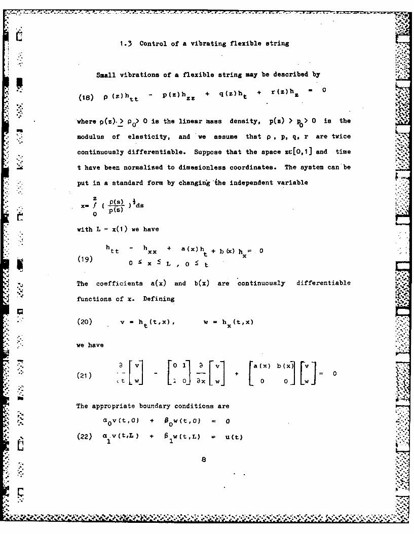
1.3 Control of a vibrating flexible string
Small vibrations of a flexible string may be described by * -
(18) p (z)htt - p(z) hz + qz(z)h + r.(z)h
where p(z)-_> P> 0 is the linear mass density, p(z) p > 0 is the0.() p0 0i th
modulus of elasticity, and we assume that p , p, q, r are twice
continuously differentiable. Suppose that the space ze[0,1] and time
t have been normalized to dimesionless coordinates. The system can be
-, -,put in a standard form by changing 6he independent variable
z I.
z p(s)%°s
with L = x(1) we have
h h + a(x)h + b )h= 0
" (19) 0 x_ L ,0 < t
The coefficients a(x) and b(x) are continuously differentiable
functions of x. Defining
" (20) v = (tx), W = h (t,x)
we have [- [0 [1 [] + x[b(x 'o [w(21) 0[. ] .] + 0
[o] 1]][~) ~j[J" t 1 3X W 0.c
The appropriate boundary conditions are
.5 % a 0 V(t, 0) + OW (t, 0) = 0
(22) a v (tL) + oW (t,L) = u(t)
8
i r.
44 %* -. ***.* 4~ 4~ ~ ~ ~ ," ** *;.** ' ;.% P
with the conditions +1, ( /$ +1 imposed to avoid
pathologies. Here $0 0 corresponds to a fixed endpoint, while
" 0 permits an end to move freely along the h axis, and a0 0,
B 0 represents an end free to move but with positive or negative- 0
• .V friction. The function u(t) is a boundary control.
One can generalize (21) to
(23) y'.. _ [ j.A.[v
with
(24[)f [a (x) a'2(x)1(24) Af = - f - al £If"-
Il a W 2 ~x a (X)21.x 22
p and the real coefficients ai j(x) are continuously differentiable on
0 x < L. By studying the finite time controllability of (22)-(24)
D.L. Russell (1972) was able to prove some interesting properties of
the eigenvalues and eigenfunctions of A. In particular, if the
* (complex) eigenvalues of A are IXk1 , then I eXk x k - 1,2 ... I forms a
Riesz basis for the space L2[O, 2L]. Moreover, there is a unique
control u e L2 [O,T] T-2L (recall that all variables are dimensionless)
which takes the solution of (22)-(24) to zero at tT2L from arbitrary
initial conditions (in the space L2 )
(25) v(,x) = v 0 (X) w(0,X) - w0 (x), 0 x L
and .
9, ..2:**-%*%..* A
-° -. -o-
IVO()I2+ IO(XI2 T ut)2
(26) kf' Ivo(x)l 2 Iwo x1 2dx : o 0 u~t)l dtlT-2.
Kf" Ivo(X) 12 + luo~x)l2 dx
for some positive constants k, K. The time T = 2L is "critical". In
general, it is not possible to make the transfer in T<2L; and for
T > 2L there will, in general, be many controls which accomplish the
transfer. By considering the special spectral *structure of the
operator A and its adjoint A , Russell was able to show that the
- unique control u(t), 0 St <2L, accomplishing the transfer could be
synthesized by a bounded linear functional of the state in (21).
From this analysis it follows that the optimal regulator problem
" for (21), that is, the problem
PO 2 L * 2 2
(27) min u (t) + fO + wt,x)I + IW t;X)I dx)]dt
%., ad
subject to (21) (22) with admissible controls consisting of bounded
(linear) feedback functionals of the state has a unique solution which
' produces a finite optimal cost. The problem (23)-(25) (27) is the
simplest example of the class of control problems treated in this
" -." work. It is a one dimensional version of the two dimensional *...:
prototype system discussed next.
1.4 Control of a two-dimensional hyperbolic system
* In an interesting paper J. Lang and D. Staelin (1982b) studied
the dynamical control properties of a simple experimental system as a
• ."prototype of an antenna design using electrostatic control to maintain
10
i.'...°°
m ~the antenna shape (Lang and Staslin 1982a). The experimental system r-
2)consisted of a flexible, conducting wire mesh (about 1 a suspended
e% vertically in tension by rigid rectangular boundaries and biased by a
high voltage source. A parallel surface of equal dimension, spaced a
short distance normal to the mesh, supported a 3 x 3 array of fixed
conducting plates independently addressable through bipolar, variable
low voltage sources which collectively served as a distributed,
electrostatic control. A similar set of plates, equally spaced from
the mesh on the opposite side, served to capacitively sense mesh
deflections. The balancing electrostatic pressures on the mesh
produced a grounded-control equilibrium geometry in which all three
surfaces were parallel.
A regulator control law was designed to modulate the voltages on
the 9 actuator plates in response to (filtered) observations of the
mesh deflections from the 9 sensor plates. Finite dimensional modal
U models representing the dynamics of 1 to 3 modes were used in the
control system design. The basic linear - quadratic - Gause'ian
regulator control law was not satisfactory in certain experimental
regimes (high bias voltage) due to 1-modeled physical factors.
Modifications were necessary to achieve mesh stabilization in these
cases. Spillover effects were also observed and compensated.
In (Lang and Staelin 1982b) the mesh was modeled as a flexible
membrane in tension. The transverse mesh deflection h(t,x,y), defined
~ as positive toward the sensor plates, satisfies
(28) mht T Th + T h~ Dh~ + f
tt 01 X Y11
Here K is (uniform) mass density, Ijt, To are (uniform) coefficients of
. a.e
mesh tension, and D is a viscous damping coefficient. Assuming a long
wave model for the electric field between the mesh and plates, the net
transverse electrostatic pressure, f(t,y,y), acting on the mesh
satisfies
V (V-u)l
(29) f j c H- - -
* *a.0 L(Hh) (H~h)2],j
where u u(t,x,y) is the potential of the actuator plates, V is the
mesh bias potential, H is the electromechanical plate-to-mesh
separation, and c is the permittivity of free space. Assuming
lhl<< H and iI << V
equation (29) was linearized, and the resulting linear control system
studied in (Lang and Staelin 1982b) was
i. (30) Mhtt =Tahxx + TShyy - Dht + Kh - But)
where K - 2%V 2/H 3and B -"oV/H2. Defining S - [0, L ,] x [0, IS] as
the location of the mesh, the mesh boundary conditions required zero
deflection at the perimeter.
If we identify Ah as the linear operator on the right in (30),
then the eigenfunctions of A are
" (31) Sn (x,y) - sin(mrx/L ) sin (n~ry/L 81
0x L -.. y L
and the corresponding eigenvalues are
12* ." a a

D2 1 2 .2
"'D D K T X n2 7= -±+ - - -.-
(32) mn 2 ;2 I14 ML 2
* These define the "open-loop" natural frequencies of the system.
Notice that the (m, n)-modo is unstable if
2 3 2 127, H T n2T
(33) V > - + -
Therefore, if V is large enough, a finite number of modes are
open-loop unstable.
The experimental system in (Lang and Staelin 1982b) has noise in
both actuator and sensor systems. This noise was represented by
Gaussian white noise. The overall performance index used in the
design was
4.L L1 1{ _i c+I)Tt LG L r2v2 '
. I (34) LM L 0 '1) [ a q 2 h 2 (t,x,y) v (t,x,y) dx dyldt}
k
where r V 01, with V0 the dynamic range on the voltage control
.i system, and q - 2 V/HvO .
The study of this small system provides a great deal of useful
information on control problems that can be expected for certain
classes of flexible structures. The control system performance
reported by Lang and Staelin provides one of the few available
benchmarks against which alternative control system designs may be
tested. We shall consider this system further in section 4.
13
l. , U, -,-, v ,, -.-.. :... , . .;.. ..: .. - ..;, -,)........,..... -,..-.......-.........,-..-,..-..--,'-..1,

1.5 Control of a simply supported beam
" .The Euler-Bernoulli equation for the dynamics of a simply
supported beam is
Mh + Dh + EIh " flt,x)tt tiX xxx
(35) o x<-L , o t
h(t,O) - 0 - h(t,L)
h (t,O) - 0 - h (t,L)
where N is the mass density (per unit length), D is a damping ratio, E U
is the modulus of elasticity, I is a moment of inertia, and f is an
applied force distribution.
If we ignore the damping, D 0 0, and normalize other parameters
to unity, then the mode shapes - eigenfunctions are fk(X) - sinkyrx and2k
the eigenvalues are k (kir) 2 . Control of vibrations of the beam, may
be based on the performance index
2 2 2 2 2"" "" (36) J(u) f [ f0(tx) + qlh (t,x) + q2ht(t,x)dx)] dt
Numerical studies of this problem were reported in (Balas 1978). A
point actuator and a point sensor
(37) f(t,x) = u(t) 8(x-
y(t) _ h (t,i 8 C* -X )
were used to effect control in the problem. Spillover into the
uncontrolled residual modes produced instability in the simulations,
14*" 14 "_
NP.1-7. -7 -7 02 -7 -7 -7- .- - - - -
I due in part to the absence of damping.
I.- This problem is considered in more detail in section 3.
15
2. Wiener-Hopf Methods for Control System Design:
The Davis-Stenger Algorithm
The connections among least squares optimization, spectral
factorization and algebraic Riccati equations have been considered
'- important in control theory for many years. (See, e.g., Anderson . -
(1967), Brockett (1970), Willems (1971), Molinari (1973a,b), Helton
S." (1976), and the references therein.) To see how the connection arises,
consider the standard finite dimensional, infinite time linear
r regulator problem .
"r f iu(t)1 2 + y(t)I 2
(I) x(t) = Ax(t) + Bu(t), x(O) = 0
y(t) = Cx(t) ,t 0
Suppose A is a stable matrix and (A,B,C) is a minimal finite
. dimensional triple realizing the transfer function
(2) G(s) = C(Is - A)-1B
Then the optimal feedback control for (1) is given by
-7.
" -(3) u(t) = -B*Kx(t)
with K the unique positive definite symmetric solution to the
algebraic Riccati equation
(4) A*K + K(A- BB*K) =-C*C
16
S. ~ ~ ?~ . . . . . . . . . . * . .* ' , .~ . ... *. .. ... . ..-. . . . . . . . .7-
An integral equation for the optimal feedback gain may be derivedj
from (4). Let a be a complex number not in the spectrum of -A*,
• : .-.*.
a(-A ), nor in the spectrum of A-BB*K, then C..
(5) K Is - (A-BB*K) .i + (-Is - A*) K = (-Is - A*) C*C[IS - (ABB*K)-
From standard results (Brockett 1970),a (A-BBOK) is contained in the
* open left half of the complex plane; and, by assumption,a (-A*) is in
the open right half plane. Let r be a closed rectifiable contour
encircling a(A-BBK) in the positive sense, and integrate (5)along I.
Since
S-- Iys - (A- B*K)J-ds =
"* (6) p..';
fr[I A*f-lds 0 0
S',we obtain
1_- -- ,---.-1-
(7) K - - A*I C*C [Is-(A-BB*K)I -ds21ri
. .and so
(8) KB - /i (Is - *]-c*c [Is- (A-BB*K)] "Bds
L7 Since the integrand is the product of two rational functions, the
contour may be deformed to yield
17
- * k-.:,.* .. * . .<~v- * .*'*. . .,. .~ :%*V..- ~ 9
?i :- S**-::*:-: . - -1-- -1 IN-1 V
KB m L[-iw- A C c*C (liW- (A-BB*K)] Bd.'.
The spectral factorization identity (Brockett 1970, illems 1971) :* "i
-1.-.,B , i w) x + Ov U w) G w) .
(10)= I+ B (1w-Afl 'C*C (11w- A]". ~(0) 1 + B* [-Ii * iw iU-l i '
...: :. = F* (1 ) F (1 ) ' ::
= [I + B* (-IiW - A*) - IK] K I + B* K (i- A) B)
and the identity
(11) C I Iiw- C BB*K)I B C (Iiw A)-B [ I + B*K (1iw A)-IB1
when used in (9) gives the result1
(12) S*K = £ IF* (iw) I B*R*(iw,A)C*CR(iw,A)dw
where R(s,A) - [Is-A] -lis the resolvent of A.
Hence, to compute the optimal feedback gain, we can either solve
the nonlinear algebraic Riccati equation (4) for its unique positive
definite solution or we can carry out the spectral factorization of
I+GOG in (10) and then compute the integral (12). In finite
dimensional control problems there may be little reason to favor
* formulation of the computational problem in one setting - the Riccati
equation - over the other - spectral factorization. In infinite
dimensional problems, however, the spectral factorization method
appears to have superior numerical stability properties over direct
integration of the Riccati equation.*
.18 e-
,4"* - ', ,,., . ,;. ."..'-.,. ° " . ," " " • - .-.* ,.":.".* . " " .*....*. * .'* ", . " .' -. .. . . .

* ' .%
&. "
VV
2.1 Davis's Method
In a series of papers, J. Davis and his students (Davis and
Barry (1977), Davis (1978a,b) (1979) (1982), Davis and Dickinson
9;- (1983)) have explored the application of spectral factorization
methods for control system design to a class of distributed parameter
models of long trains with multiple locomotives. The control problem
is to modulate the acceleration of individual locomotives to minimize
deviations in coupler stress throughout the train. Disturbances
include passage of the train over a grade, which tends to set up a
"travelling wave" along the train of stress deviations from nominal.
The first approach to this problem which comes to mind is to write out
the equations of motion of the cars and locomotives in the train and
formulate an optimal control problem for the overall system. The
large dimension of the resulting model and the absence of any special
structure inhibits this approach. Decentralized control schemes
(McLane, Peppard, and Sundareswaran (1973), Gruber and Bayoumi (1982))
- .are not particularly effective for these problems. As Davis and Barry
- "(1977) have observed, aside from the difficulties in solving large
scale control problems, one has trouble estimating the effects of
system parameter changes or of variations in the number of units in a
block based on lumped parameter models.
Davis recognized that the mass-spring nature of the
interconnected system could lead to traveling wave phenomena setup by
19
%.!%
"competing" local controllers (locomotive accelerations), Hie reauoned
that the macrosopic, widely coupled motions of the elements would
contain the bulk of the energy of motion of the total system. This
hypothesis suggests that a control scheme designed to suppress such
motions would achieve substantial reductions in the coupler stress
levels.
To represent the system in a fashion which would capture wave
phenomena most naturally, Davis reformulated the system as a
distributed parameter system with boundary controls. (Davis and Barry
1977). The resulting model proved to be mathematically tractable.
The effects of changes in both system parameters and the number of
units in a block were readily apparent. In fact, an increase in the
number of elements in a block increases the validity and usefulness of
the model. In contrast, finite dimensional models tend to become
increasingly intractable as the number of units in the system
increases.
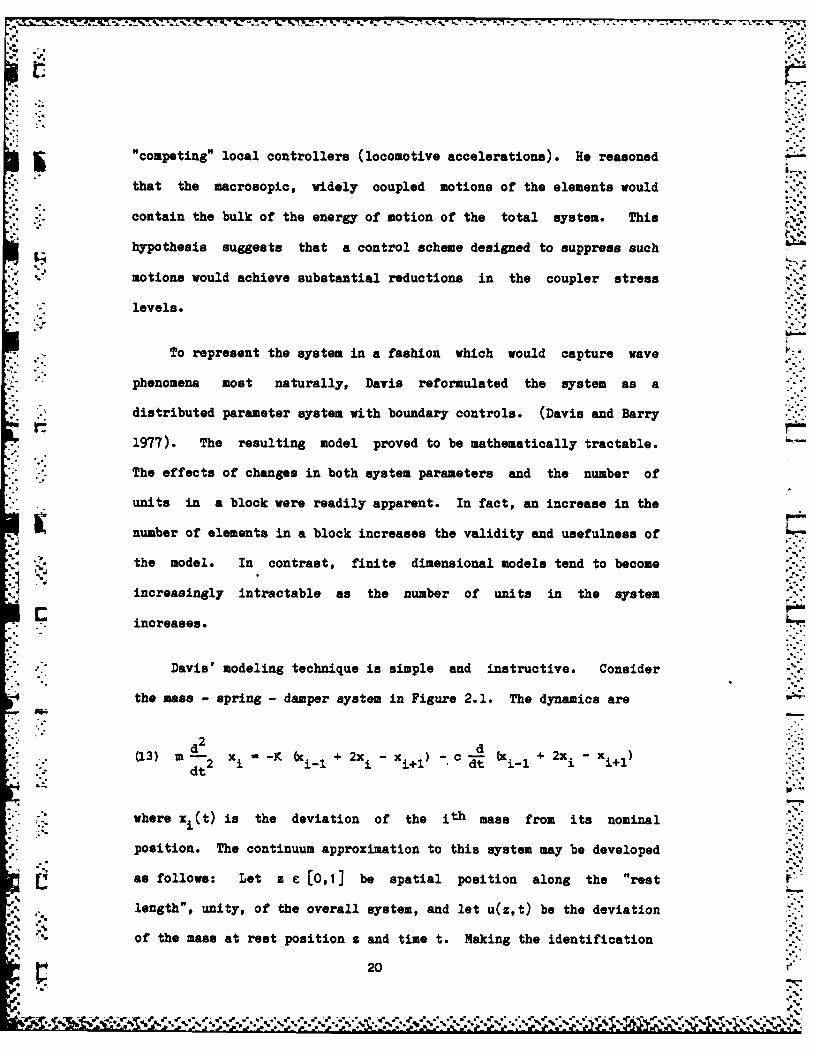
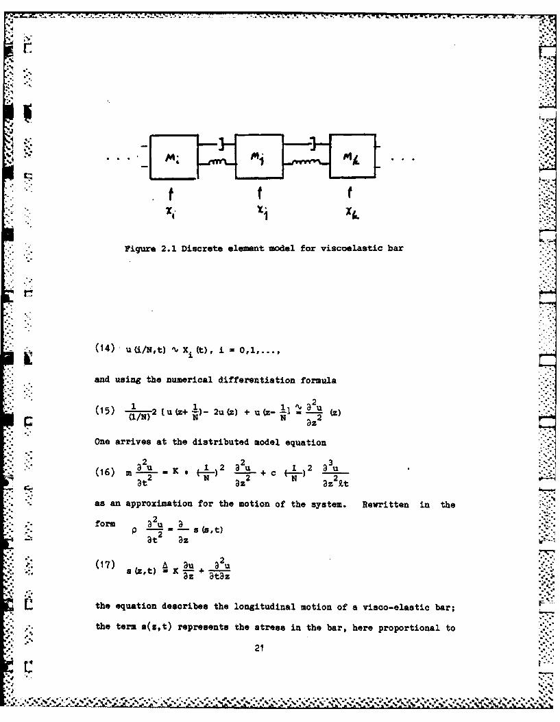
. Davis' modeling technique is simple and instructive. Consider
the mass - spring - damper system in Figure 2.1. The dynamics are
d 2 d ,..
3)m- x -- K (X + 2x -X )-c X + 2x -X )dt2
: -1 i i+d i-i i
where xi(t) is the deviation of the ith mass from its nominal
position. The continuum approximation to this system may be developed
as follows: Let - e [0,1] be spatial position along the "rest
length", unity, of the overall system, and let u(s,t) be the deviation
of the mass at rest position z and time t. Making the identification
20r. TV
}re~ %L%' %
_mm L.
Figure~~~~~ ~ ~~~~~ 2.1Dsrteeeetmde.o.icolsi a
(1 )u4.N t
On rie t th ditiuetodleuto
2 2 3
at z
Oae arrivesatithefdistiued moel ofeatewitenh
223
at 2Z azz
2~form au a uat az aa
the equation describes the longitudinal motion of a visco-elastic bar;
the term s(z,t) represent. the stress in the bar, here proportional to
21

a linear combination of the strain and stress rate (Davis and Barry
1977) (Greenberg, MacCamy Nisel and 1968). The natural boundary~.;
'? , : conditions for (17) are in terms of s(zt) at s-O and 1, i.e.,
-;" (18) s(o,t) fo(t), s(1,t) f Qt)
the applied forces and u(z,t), u (z,t) at t-O.t
Rescaling time at t' - t/k/c), the system (16) may be rewritten
in dimensionless form as
(19) ;- a +_2_ + O<x<lt<(19) a2 a z a
with a - c2/kKN3. And this may be written in matrix form as
['at u a OaS, ~(20a) La LI"
(2b N 1 U + uz](O't) f- (t)
Na lux ut)1t) Y 1 t)
,(o), u(zO) given
Let A be the matrix differential operator on the right in (20a).
Defining H IPL[O,1] x L2E,1] with the energy inner product,
.....
22us u ],'.' 9"

.. -.-.'
* q
(2) < ' > (sCup + vq) dzv q 0
(21) < f:] , r I - Po (au:.q d
then A on H has domain
D(A) - {[U]: u,v,v absolutely continuous u ,v eL (0,1],
(22) " -"u + V = 0 at x = 0,11
x
dense in H, A is a dissipative operator, and A is the infinitesimal
generator of a class C contraction semigroup T on H (Davis and Barry0 t
1978, Theorem 1). Moreover, the resolvent
(23) R(s,A) 00 e Tt dt.
of A may be computed explicitly. (See section 3 or Davis and Barry
1978.)
-- V
. ,. It is not possible to write the solution of (2) in the strong
form "
• " ,".(24) " = AU + Sflt)(24) -r+ft
where
T T(25) R nff
2B:R - I. H -'.
since the boundary forces correspond to generalized function "inputs".
Using L "1 as the inverse Laplace transform, Davis and Barry treat (20)
Si. n the form
(26) U(t) - T U(O) + L 1 {G(sgz) f (z)t
- . 5. - .23
. *- ,.1 , . ,?' , . , , .,*.1 ,_ . ', *,, V_. _ .. .. .. - .: - '-.-.... .' - -

I - 7.F 7 77.- ZI-...7-r-i-7
-S where G(s;z) represents the "transfer function matrix" associated with
the boundary value problem (20). -'.
The (optimal) control problem involves minimizing variations in
the stress distribution throughout the system. The quantity .
1 12 2"'12's2 (z,t) dz- at + .'"-z.'"a/
V, (27) 0 ,a
corresponds to the total stress in the system. Recalling the original
approkimation(13)-(16), we have the correspondence
1 2 2 Nx C 12
(28) f0 (us+ Uz) dz N X X + (X X0 z zt i i M-x
and so, the natural quadratic cost functional is
(29) J_ {Ifo() 2 + If12 + 1fo (u + u 2 d-}dt
This formulation includes stress contributions from spatial modes
of all wavelengths. In most physical systems high order modes will
". .- - .'-A *have a negligible contribution to the overall behavior. Using "r to
denote projection onto the subspace of H spanned by the first p
- eigenfunctions of A, and defining the system output as
(30) Y(zlt)- OL"r. [• 1 (z't)
the final formulation used by Da-is and Barry (1978) is
[7 { If0 (t) 2 + If (t) 12 + fy (z,t) 12dx} dt•~~ f ( ) n 0- - -
00
24L4 .... ,
-: t.... . ... . . .. . . .. . . .. . .A. ... .'. %. . .

it:%
U(.,t)- T, Co) () + L {G(s, (Z), (t,
y(z,t) - a[l,a ] [ U] (z,t)z p2 2
U(0) C D(A)C.L [0,11 x L [0,1]
The resulting optimization problem is a distributed control problem
with state cost restricted to a finite dimensional subspace.
Davis and Barry (1978) compute the optimal control law for this
problem using the spectral factorization algorithm described earlier.
A key step in the procedure is application of a numerical algorithm
for spectral factorization due to F. Stenger. In the next subsection
we summarize Stenger's algorithm.
2.2 Stenger's Algorithm for Spectral Factorization
To evaluate the control law for a given problem modeled as in the
last subsection, we must compute the spectral factor F(s) appearing in
equation (10). That is,
• *
(32) F (s) F(s) H(s) I + G (s) G(s)
where G(s) is the transfer function of the system being controlled.
The first problem is to determine conditions under which the spectral
factor exists. Since G(s) is the transform of a real vector valued
function, which we assume to be integrable and square integrable, it
follows that S(s) - G*(s)G(s) is a Hermitian positive semidefinite
(matrix valued) function and G*G is the transform of a function which
is in LI/ L2 _
25
-*. ,"Ile %L
L a -:>.. ',-;~S~ ~S .5

oIw
S ISince S(s) is the transform of a function in L2it follows from
the classical theory of Gohberg and Krein (1960) that H(s) has a
'S unique spectral factorization of the form (32) where
tl +F I £ F (L+) C-Fourier transform of L, flaCtionxs)
F U40) - F(-iad)
where L4 denotes those functions in L with positive support. As noted
S in (Davis and Dickcenson 1983), the assumptions on S(s) in fact imply
(34) F 1 C F(1fL 2)L
Sand F(iw) F(P-iw). These conditions, therefore, settle the question
.' . o.
of existence and uniqueness of the spectral factor.
In (Davis and Dickenson 1983) an iterative algorithm was given
for computing the spectral factor. Since this method is at the heart.
of our computational programs, and since it makes use of Stenger's
algorithm, we shall develop it here. The starting point for the
iteration in (Davis and Dickenson 1983) is the Newton-Raphson
- iteration for the solution of the algebraic Riccati equation (4);
that is,
:'"(35) n±l z * n' .l * n n:::
K (A BB K + (A- BE'
From this a simple calculation leads to the desired form of the
iteration for the spectral factor (see Davis and Dickenson 1983, pp.
5 290-291)
(36) F~~ P HPF)- S(F~) 1 F
.
= , °-.4.%t~.4.P.~4
. , __
whre Po[puti s the pcaual prjetnoprtor. Sidti e fine on ther
-_ ';ofou cmptatonl rorasandsiceitmaesuseofStngr'26
W .. ; :
1 2convolution algebra I0 L1 or on L "by
(37) P+ [I + f(t) e ldt - I + f f(t) e tdt
Stenger's algorithm is used to provide a numerical approximation to
the causal projection operator. Before discussing that, we note that
. under the assumptions on G(s), and therefore on S(S), that the
iteration may be shown to converge from a suitable initial guess to
2the uniquely defined (in L causal spectral factor F(s).
The algorithm (36) has a particularly simple form. As noted in
(Davis and Dickenson 1983), the computation of P+[-] is the most
• difficult step, but Stenger's result takes care of that. The
numerical approximation in (Stenger 1972) takes the form
(38) P4 If] I M (W). f(kh + ih) r h)) t ( k m (w-kh-ah).
Here h is the step size and r and a are parameters defined bym mStenger. Specifically,
(9) a r 4k __h__ 2M 1i m m 4kJK qC
r--i
where q is a parameter chosen in the algorithm and
2 2(40 xK (a/b) k - }xb2
- ~(40)k-w
an 2~ q b 1) +i2+ Z qm" - (-l m-l-..
m~l m~l .-.. '
27
Sle= n%. ,

7 17. 07 ,°-.°-
The step size is chosen based on the bandwidth of the transfer
function 1(s). If, in (38), one chooses to sample the projection f* .. A ° '
at the same sample points as f, then, as observed in (Davis and
Dickenson 1983)
..(41) f+(kh + fjh) f + m--
(k-j)h-a h + Jh
and it is clear that the required calculation is a convolution. Since
the range of sample points is finite this is naturally implemented by
a fast Fourier Transform (FFT); and this substantially improves the
computational time.
r-K Since we must compute (F*) S(F )- in the iteration (36) for theSI n n
spectral factor, it is best to rewrite the iteration as
(42) (FU- - (Fn)- ( + P+ [(F S(Fn ) -i]) -I1
and execute it in this form. As observed in (Davis and Dickenson
1983), the last factor in this expression is a perturbation of the
identity* (since (F*)-IS(F )-1 - I 0), and this has naturaln n "
advantages in the numerical realization of the iteration.
As suggested in (Davis and Dickenson 1983), a suitable choice for
the initial guess for the spectral factor F is the diagonal matrix
whose elements are (scalar) spectral factors of the corresponding
diagonal elements of S. This choice implies that the matrix
(F*)-Is(F )-1 is a matrix with ones on the diagonal and with all then n
off-diagonal elements less than one in magnitude. This tends to
prevent the iteration from blowing up. The diagonal factors may be
28[.. ,°'72

obtained by an FFT implementation of the scalar algorithm in (Stenger
1972).
The method as described here was implemented directly on the
problem of controlling the dynamics of the Euler-Bernoulli beam. The
results are shown in the next section. A careful consideration of
Stenger's method suggests an alternative implementation of them0
algorithm which takes advantage of the occurence of Hilbert transforms
in the course of the computations and the effective use of these
transforms in the representation of the causal spectral factor. This
observation permits an efficient numerical realization of the spectral
factorization procedure. We shall develop this in the context of
design of stabilizing controls for a two dimensional flexible
structure. This result and the associated algorithm are reported in
section 4.
2--,-.v
• -.. ° . ..
. . . . . . . . . . . . . . . . . . . . . . . . . .. .. '..... . . .
~ .~<yC *. .. ~.*.:-.:-.-;*.:* .:-.:* .. *..-. * .- ~ -: ~ ~ :, .- , *.... . . .--
-.. ..... . . . . . .'.-. - .-.-.- .."..- . P . -,
3. Control of a One-Dimensional Structure
The control of simple one dimensional structures serves to
illustrate the general analytical methods in the simplest form. Onedimensional models can also represent certain components, e.g.,
flexible beams, which appear in composite large space structures; and
they may represent certain two or three dimensional structures with
natural symmetry. In this section we consider a simple system, the
Euler-Bernoulli beam in detail working through the computation and
simulation of the optimal stabilizing feedback gain.r3.1 Control of a Flexible Beam
The dynamics of an undamped flexible beam undergoing transverse
notion are described by the Euler-Bernoulli partial differential
• .equationm ut (t,x) + EIu (t,x) f(t,x)
XXX •
1E(1) o <x < L, t>o
where u(t,x) is the transverse displacement of the beam, f(t,x) is an
applied force distribution, m is the mass per unit length, I the
- moment of inertia, E the modulus of elasticity, and L is the beam
length. To facilitate comparison of our results with earlier work
(Balas 1978b), we shall assume that m, E, I, and L are all unity. The '.
boundary conditions for pinned support are
u(t,O) = 0 - U(tl)(2)
u X(t,Q) =0 -u_ X(t1l)-
" :] The beam is controlled by a single point actuator
30V .° % .'
%4 .- ,--o -
(3) f(t,x) - 1 (x-a)v(t) O<a<l L
and a single sensor measures displacement
(4) y(t) u(t,b), O<b<l
The system is deterministic and actuator and sensor dynamics are not
modeled.
Balas (1978b) designed a feedback controller for the first three
modes of the beam which minimized the (unweighted) energy in tnose
modes. His controller includes a six-dimensional Luenberger observer
to reconstruct the state.. The energy in the fourth (residual) mode
increases rapidly due to spillover effects.
Our approach to this problem is based on the infinite dimensional
model. Taking the Laplace transform of (1), we have
U xxxx (s,x) + s2 U(s,x) - F(s,x)
(5) U(s,O) = 0 - U(s,l)
U (s,O) = 0 -U (s,l)3= 0
the Green's function for (1) (5) satisfies
(6) G (s,xjx") + s2G(s,xlx') -(x-x')-
Consider G in the form
fA sinh ,/ X) O<x<x' -.
(7) G('s,xlxb .sinhf (1-x)) x'<x<l
with A and B complex constants to be determined. Note that the
31
a~~~~ -.. . .:.i, - --- - - . &z. -
. % .
boundary conditions in (5) are satisfied by (7). At x-x' we have
G (8) + s G dx=UI
- mx 'I -I
(See Tai (1971) F From (6) (8) we have
x' +e(9) G I =1
r and from this
(j~ N -1 (5mb s (1X
B ) s3/2 sinh s sinh s x' /
which gives the Green's function. -.
The transfer function relating the input f(t,x) in (3) to the "'.
" . output y(t) in (4) may be written down immediately from G(s,xlx').
, fl C(r,xjx') F(s,x')dx' = - G(s,bla) V(s)""(11) Y(s) ff U(s,b) = foI"-
with V(s) the Laplace transform of v(t). Identifying
we have
32
'. . .*. "-"-"'"~ . .","'".'H ."771 F..5 . . % .
-(sinh a a) sinh (l-b) s)r'"3 /2 ~, x -a<b-x. -" 4 / 2- -3 / s n h / -"--
,:-~ ~ 31 ) T a (S) - :
-(sinh (1-a) s) (sinh b s)fi-3/2 i-a>b x
Balas~r 198us s = "::
Balas (1978) uses a b and for this case we have
6 6|2(14) TB (s) T (s) 2(sinhjs/)
:IB 13/2s2s sinhf a
To use the Davis-Stenger algorithm as described in section 2, we
must compute the spectral factorization of
(15) H (s) 1 + TB () TB (S)- F (s) F)
Substituting, we have
2 2
(16) H~iw-l+~ (sinh/ 6) (sinh !;i/6)
and the computational problem reduces to computing the spectral factor
F*(s) from (16), and then computing the optimal stabilizing feedback
gain
* 1 .-.. *. *
(17) BK [F* (iw)] G () CR iw, A) dw
by numerical integration. -%
33
L.; ,....| . . .- ,

L- .7* ;-.7 -U.-*
* 3.2 Numerical Results
In the computations and simulations which follow, we consider the
same beam parameters used by Balas (unit length, with parameters
normalized to one, and zero damping). The numerical requirements of
the algorithm are not changed for more realistic choices of
parameters. In addition to the case considered by Balas (with one
controller and one observer at opposite ends of the beam), we also
consider the effect of increasing the number of controllers and
observers, and finally the effect of delays in the control loops.*
Practical implementation of the algorithm requires frequency
sampling of the transfer function and spectral factors, and spatial
and frequency sampling of the resolvent. It was determined
experimentally that for the given beam parameters, a frequency range
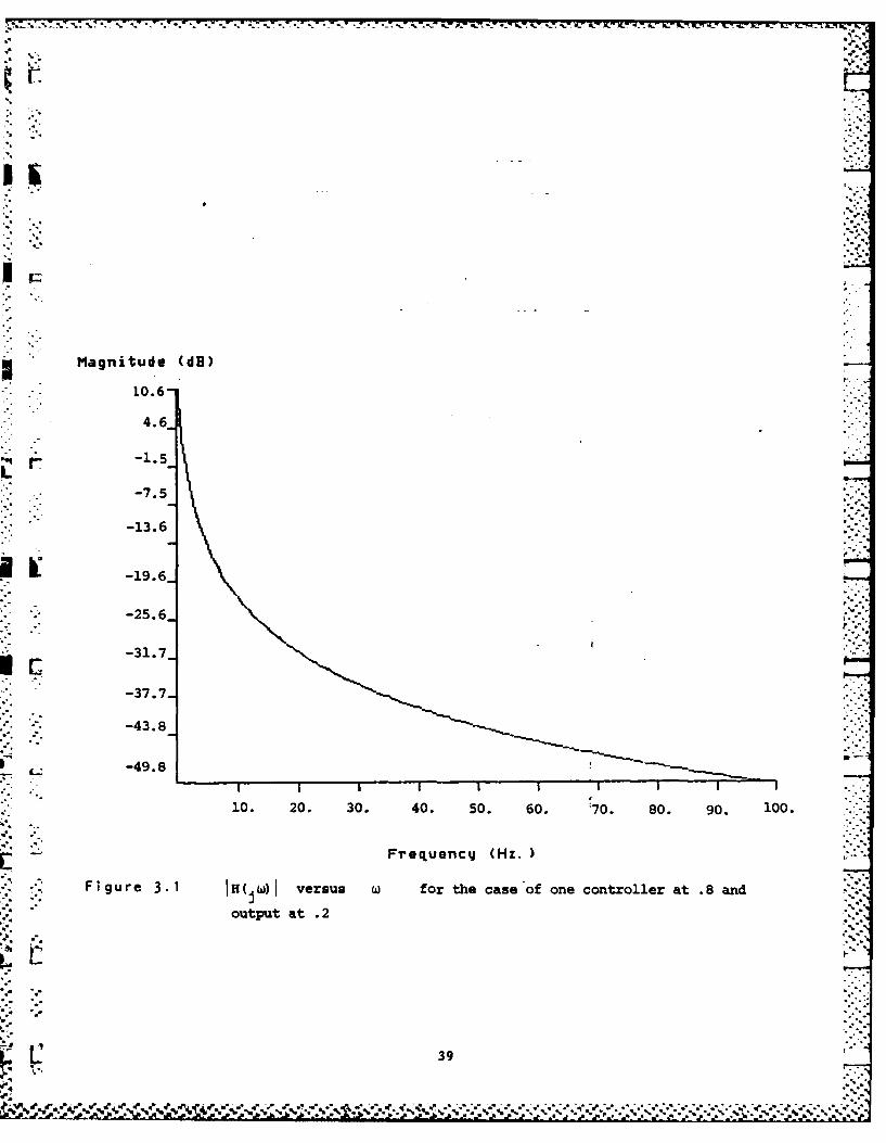
of plus/minus 30HZ is adequate, since the gain from input to output in
the range beyond this is insignificant, see Figure 3.1. The figure
also indicates a very smooth dependence of the transfer function on
frequency, so that the 256 sample points used in the program are quite
adequate. Spatial discretization is done using 100 equidistant
points.-
An example of the feedback gain is given in Figure 3.2, for the
velocity state variable, and in Figure 3.3 for the displacement state
* variable. (See Appendix A for other gains corresponding to different
*The issue of the effects of the delay on the control action andthe system stability was raised by Dr. J. Burns, formerly withAFOSR, and now with VPI&SU, Blacksburg, VA. We are grateful toProfessor Burns for his inputs on this problem.
34
arrangements of the controllers and outputs.) A sharp peak at the
point of observation for the deflection state indicates the control
effort to reduce the deviation at this point to zero, since only this
point contributes to the optimization cost. In this case we have
penalized the state deviation at the observation points (in the cost
criterion) 500 times more than the control, so this is "cheap
control."
The feedback gains, one for the speed state and the other for the
deflection state are integral operators as defined by (17). These
gains are computed off-line. Computation of the input function for a
given time requires evaluation of the integral operator B K acting on
the state. This is accomplished in the program by approximating the
integral as a sum of piecewise constant functions.
In controlling a physical beam one would need an observer for the
deflection and velocity variables that would use (point) observations
..of the beam deflection as inputs. For the simulation results here the
deflection and its derivative are obtained by numerical integration.
S*'" The case studied by Balas, where the controller and the observer
are at the opposite ends of the beam, exhibits poor observability and
controllability, which is reflected in the large control efforts and
long settling times to stabilize the motions (see Figure 3.6). Using
more observers and controllers substantially improves the
"controllability" of the system. For example, in the case of three
collocated, equidistant controllers/measurements, the margin of
improvement can be seen by comparing Figure 3.5 with Figure 3.6. See -
35.
. ~ ',..* .h/~..v .- ** - .. .~:s:. f..f /.~.j .Au .. LiL,~% AL%.~ VV
p.o. * .o
also Appendix A for the time responses corresponding to these two
cases.
Delays in physical control loops are inevitable due to the finite
time necessary to process measurements and compute the resulting
controls. Analytical treatment of delays using time domain models is
not nearly as convenient as it is in the frequency method described
.. here. For example, if the delay is T, then we need only multiply each
.. .- element of matrix H(s) in (15) by a factor exp(-sT). Therefore, H(s)
is invariant with respect to the delay, and the critical part of the
gain computation algorithm, i.e., spectral factorisation, need not be
recomputed for the delayed case. Of course, the delay appears in the
transfer function, and so, a new gain must be computed for each
* - different delay. (Numerical results displaying effects of delays are
discussed later.)
' To validate the program, we simulated the response of a beam
subject to an initial disturbance in the form of one of the spatial
modes, and with a feedback based on the optimal control discussed
above. Figure 3.5 is an example of a time variation of the beam at
the observation point. (Other such examples are given in Appendix A.)
Note that without the control this response would represent an
undamped oscillatory motion since the beam model does not include
damping. Damping has a stabilizing effect in this system; and the W.,
control action is enhanced if damping is present.
.: . ... ,3
• 36 -
The plots summarizing numerical work o h xml rbe
.C., n th examle poble
appear in several groups in Appendix A, and they are grouped asL
follows. For a given delay, an4 a given number and position of
V ,~ controls and observations, we first display gains for deflection and
velocity states, both for each of the inputs. Next is a group of
~ plots showing the beam response to the optimal control when the beam
is initially displaced in the form of one of the first three spatial
modes. (significant components of the matrix H(i )are well below
30Hz, i.e., below the frequencies induced by the 4th spatial mode.)
The meaning of the plot titles is as follows: "Beam at x, yth mode,"
t means that the beam is initially displaced by the y-th spatial mode,
and the deflection of the beam is observed as a function of time at-
point x. On the control plot we indicate the position of the point
control and the time evolution of the control at that point.
While the main purpose of conducting these experiments was to
verify the control algorithm, several phenomena were observed from
these experiments. Comparing responses of higher order modes with
those of the lover order modes, it is evident that more energy is
* needed to control higher order modes (note that our model has zero
damping). This reflects the poor controllability and observability of
the higher order modes. Second, the gains for the deflection state
have pronounced peaks at the observation points, suggesting use of
localized - decentralized feedback. Unfortunately, the speed gains
* indicate much more spatial, coupling, suggesting that decentralized
* control schemes may not be effective (at least for the parameter
ranges used in this problem). Third, the delay has a substantial
37
-- . -. .- ._
effect on the performance of the control. (Compare any case with
delay from Appendix A with a case with no delay.) Nevertheless, the
stability margin is remarkably wide. An example from Appendix A
indicates that a delay equal to one half period of the highest mode in
the chosen spectrum does not destabilize the system.
The numerical results presented above affirm the Davis-Stenger
algorithm as a practical tool for vibration control of flexible
structures, represented here by an Euler beam model. The results of .
this algorithm provide a means for assessing effects of
controller/observer placement on the system performance, as well as
give stabilizing feedback gains, once the controller locations have
been selected. It was also demonstrated that the underlying model
allows an efficient treatment of delays in the control loop.
38- .
:. ::S
8 "-.'. ''.'.0
, •.".//.-, ',-'" ; .".. .." " .: .,'..' -;.'.....-'..' - r -- : ." -, .- - '. ;'.'.'...; -... '
Magnitude (dB)
10.6-
4.6_
-7.5
-13.6
U h.-19.6-
-25.6_
-31.7.
-31.7-
-3.7
-43.8
10. 20. 30. 40. 50. 60. :70. 80. 90. 100.
Frequencyj (Hz. )
Figure 31 J(wlversus w for the case'of one controller at .8 and
output at .2
39
GA IN
1 .128
.112
M .096
.08
lh~ .069
.048
.032/
.016
0.
.2 ij .4./6 . .8 .POSITION
F FIgu re 32. Gain profile for the velocity state; Actuator at .8, output at .2
/40
%e te

..
GAIN
0.
-. 4
-.8
-1.2
* -1.6
* -2./
-2.4
* -2.8
-3.2
.1 .2 .3 .4 .5 .6 '.7 .8 .9 1
POSITION
F ig u re 3.-3.- Gain prof ile f or the def lection state; One Actuator located at .8,
output located at .2.
£41

*GAIN
0.
r6 -. 56
-. 84
-1.12
II -1.40
-1.68
-1.96
-2.24
*.1 .2 .3 .4 .5 .6 .7 .8 .9 1
POSITION
F ig u re 3. 4. Gain prof ile for the def lection state and f irst output; three
collocated actuators/outputs.
K 42
Beam at .2; 1st mode
DISPLACEMENT0. DOGtE-01
-0. 197E-01 .1 .2 .3 .4 .5 .6 .7 .8 .9 1
TI ME
Figure 3.5. Time response of the beam; three actuators.

Beam at . 5; 1st mode
DISPLACEMkENT0. 100
I. -
T I H L
a.° -
'a'.
Figur 3.. TmBepn e m of t beam; on autm o r.
• .-
0. PLCHN "00':"0
; O.TI O0
" .."- .... °.'
-" , -k.-
4. Control of a Two-Dimensional Prototype System
In this section we adapt our frequency domain control system
design procedure to treat a prototype two dimensional flexible system
! "- - a membrane/mesh whose dynamical behavior is sensed and controlled by
S.electrostatic forces. The model is patterned after an experimental
system studied by Lang and Staelin (1982b) as a paradigm for an
electrostatically- controlled large aperature reflecting satellite
antenna.
While the starting point.for the control system computations is
similar to that for the Euler beam, our analysis takes a somewhat
different tack. We shall exploit the appearance of Hilbert transforms
in the derivation of the spectral factor and the simple way in which
these transforms can be used to represent the spectral factor
appearing in the expression for the feedback gain. As we shall see,
there are some significant computational advantages obtained in this
modification of the Davis-Stenger procedure.
In the next subsection we describe the model and compute the
transfer function. In the following subsection we write the solution
for the mbsh dynamical system in terms of the eigenfunctions of the
evolution operator. This provides an effective and accurate basis for
numerically simulating the (controlled) system dynamics. It is
superior to nuwerical solution of the PDE model by finitq difference
Mmethods.
45
L "'o.4h .%. .. **:*" .. |. ~

..- .:.:.,-' - -.
r-7
4.1 Dynamics of a Vibrating Membrane
The physical structure of the prototype experimental system used
s by Lang and Staelin (1982a,b was described in section 1.3. We shall
describe the mathematical analysis of the system here. The linearized
equation describing the dynamics of the voltage controlled mesh is
32h T 32h T 2 2O O
at2 .. 2 2 2 M. at .'-W
h=O on boundary of [O,L) x [O,L-
h(O,%,0) ( 0, h: (0, ,) - 0"t
where the boundary conditions reflect the fact that the mesh is pinned
along its boundary. To reduce the computations, we make a change of
coordinates to remove the derivative term in (1); that is,
:i+_ (2) h (t) f (t) exp, --H t} .?.
2M22CL
We obtain 92 f Ta 92f T a a - 0 2C C 0 }--w .W- . -2 U t v...t2 N3 2 J4 2 4 3 H2 2m
(3) f=O on boundary of (O,L] x [0,L]
f (oct,B) = 0 ft (0,0,) = 0
Let us define thi parameters
-.. Y~2 2V/- "3-.'
(4) a:'= T/M, aB a T8/M, 2- 2""V-/M.-
(4)0 -w
-au -- expp t V
and using these in (3) we obtain
.• .*o o..•'
46
"- J.. ". .
+':: : N..-,
; "- *, '**' ' " ," "t* "- " ",%",.""b % .> " "- ".' '"-.-' -" " " . '''- .."" .. :. ;' ':" -" ... / ?:@

3 2 ,a_ 2
2 - s, 2 a ~2 y~at a(5) f 0 on boundary of [O,L x [0,L]
f ft -0 at t -0
It is possible to reduce the equation further to the standard form for ."
wave equations; but we shall not do this since it will complicate the
boundary conditions.
Taking the Fourier transform in (5), we obtain
2 2p2(-iw) F()= a - 2 - + a t + YF + au
F= 0 on boundary of [0,L] x [O,L] -
By splitting F and U into real and imaginary parts, respectively, we
are led to the following equation
} 2 H a 2H 2-'
(7) a + a H- + 2+W) H- -a v
Our immediate objective is to find the Green's function corresponding 6,
to the boundary value problem (7).
To accomplish this, we shall reduce the problem to a one
dimensional Sturm-Liouville problem. Consider the operator
2 2*'. L~ U-a a u-"w
.':- ". (8) .-
with u (0) - u(M) = 0
Using this in (7), we have
a -2 H L H--aau
H - 0 on the boundary
Lt 47
-Z; Z Z...

- -0 7 .7 -a -
3 and so, the Green's function satisfies the PDE
a K
* -: (10)*
K -0 on the bonayof [0,2.] x [0j2]
Let (c.) be the eigenfunctions of the operator L., ,
We shall compute the Green's function in the form
-k-1,' (lO) ,'.'-F'Tl);."~k
We define the weighted inner product
(12) < the> - f a ctos f where ope [ o x I
Substituting the expression (11) for K into (10), we obtain
...
-, (13) a , a"(n ) ' k ('6k ( ) ) (8-T)k.k=1 k-i k
E': WBut ( n) are eigenfunctions of L
(14) Lk (ac) =k a, k (a
Multiplying both sides of (13) by( ) , J k and integrating over-
we obtain
"* ': (1 [ a" (8) ( 0 (a) - -\(a .- () (- ** ,..;:-] dc
0k i k k l 0 .:).-.:(a"(15) 0
L- -I (ac~ 6(8 -TI ) dci
0
which implies (using the orthogonality of and the properties of the
delta function)
48-
• -. /
a .1 .a.
%* -S.-.,
(16) . :.
ak(O) = akL) -0
This is a classical Sturm-Liouville problem.
The eigenfunctions of the operator L satisfy
.(2 2"- L% =X k k* ,a* " - .::'
(17) ,
(0) - *k( ) - 0k k
It is a simple calculation to show that the eignevalues are
S(18) 2 n- ,2,...aa n.-.r'(1) n a a,
and the eigenfunctions are
2
(19) n 0) in (n W t) n= 1,2,...
Nov we have to solve the Sturm-Liouville problem (16). Referring
to (18), we have to consider the three cases: X > 0, X - 0, and
X < 0. Note that for each fixed w there is only a finite number of
negative eigenvalues. To solve (16), it suffices to solve
a" - Xa 6(a- n)(20)
a (0) =a (V) =0
We have dropped the indices for convenience and the term M ( ) whichn
.'. -'. will be handled by multiplying the resulting Green's function by the,..:.
same factor.
49
....
Ca se 1: =? .
It is a simple matter to show that the Green's function
associated with problem (20) is
(2) G (cr)) 1 sh ( -n)) Ash vB) 6<0<r.. .- (21) h sh I h41(, ) I89Ush
where sh(x) - sinh(x). To obtain the desired Green's function
associated with (16), we simply multiply (21) by (E). This gives
2 sin Sh ( sh" '") <a<_ _ n
"' i (22) Gn ' = s n . l s n )_ ',"
z. 1 sh 41 Z) sh (1 n) shlIn(L-I)n<8<"n n L n -n
where ui
2<Case 2: X=- <0
. -Arguing in a similar fashion we find that the Green's function
-' associated with (16) for this case is
2: ' , i n e 7 ) s h P ( k - f ) ) s h (p ) o < a<. .
(23) Gn ' " inSh .n £) sh n h n -8)) n<8<..
4° .1'
50
.3 ." :."j:AI
" -" Case 3: X-O
In this case the desired Green's function is
/2'sl ( t -r) o<B<n . .
(24) G (8,n) C .) _
Note that (22) and (23) can be given by the same formula if we
take n to be a complex number (either ih n I or I 1I). Also, (24) cann n-n
be obtained as the limit of either (22) or (23) asR n 0. However,
' it is best to split the expression as above to maximize computational
efficiency. The procedure we have followed in representing the
Green's function has two advantages over the classical expansion of
. the Green's function in terms of eignenfunctions of the whole problem
(as used in Lang and Staelin 1982b) First, it reduces the
expression of the Green's function to a single sum instead of a double
sum as in the classical representation. Second, the series has a
strong convergence property. Since there is only a finite number of
negative eigenvalues, the main part of the series is given by (22)
which can be expressed in terms of exponentials. This series
converges exponentially fast. In fact, the bilinear eigenfunction
expansion for the Green's function fails in this case since X0 0 is
an eigenvalue for an infinite number of w 's, and the series diverges
in these cases. The complete expression for the Green's function is 4
-. 51
e.Z-

.o- .,'_.:""L"". "" ." -. " - . .- - - . _. "-- .--- J -- --- , -. 'o '-'- -°
'-" .~ -- .- -V . r r r r r U-I V- ' . ' , , . . . ..
n1 2.- n no
';. " sin. A i 1..(25-: ) + E noj 2 c - n) .:,>
i -Ci)
sin ~ ~ Si ) sn 41(-T snWn
~Here we have used the notation " .
;:[ (26) no- = rw/
""1
k-i and [no].is the integer strictly less thatno, including the case when .-.-.
.it
i an intger. Also,
:
U0 not integer:- -. (27) £[nJ= 0
and•
..(28) snn = 22 - n,2,"
,.. ~Finally, note that the Green's function has the symmetry property ..-.
;'. ""(29) +,, ,8, ,n) K(?,n,ct,8) for n91<< "I
52 _52
• "..=.'.T) " .
,% . . . ,- , . ," e o , , % . ,, % % .& . , . . % , % •, , . . . . o . . . % ..a.•~~~ ~ .'a sin sin . .. sh' (A-11), s.h 0) _ ,',_ ,-,OPZ%' .s.'.." ", w e P4 , ,. .,. ,W.O ",T,,@'
*7 .7 7.- 7 - 2- -- 77°
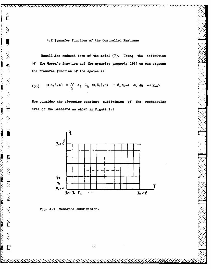
4.2 Transfer Function of the Controlled Membrane
Recall .the reduced form of the model (7). Using the definition
of the Green's function and the symmetry property (29) we can express
" '- the transfer function of the system as
(30) H( a.,,w) W ) f aB (O L,Bo, n) u (F,,lw) dE dn =<K. >(
Now consider the piecewise constant subdivision of the rectangular
j I" area of the membrane as shown in Figure 4.1
?A
- ' -.1
"i' "-- - -'"-"
.* . r.@... ho*
Fig. 4.1 Membrane subdivision.
53"

. %...:--.k
I 3 Assume that the control input is constant over each small
rectangle
( |)~ Iit =[ I i l X [ j, n + I] i,j, 1 , ... ,N"'".._.-.-
That is,
(32) u (,Te)=uij ) for i <i+l
Using this, the transfer function can be expressed
" - H ,8,W) 1ff a (ct,8, ,l) u. , Wth,) d dfl -
*.. (33) N N
iB . a u <T&ljf.....'d:d.i-l J 8 1
" . To compute the integral over f2"- it is necessary to distinguish
three cases: 8 < j., 8 > nj+ 1 and 8e I nj nj+ -"'"
Case 1: 8 < T-
Substituting the expression for the Green's function (25) into
" "(33), Ye obtain.w,-. ff i ,8 ,n d~df .. :
ii [
." .2 ff 2. sin )sin Tr a sin Q/n (in)) sin 41n6)d~dr"2 nij niln
.. ,.;n-1 z n
ij V s ?-'-. nk)
(34)"n 7r
t~~E sin E) "sin ( , (-)dtdn "-
,[.: Z :"F si ( "L".j
,=. -: i ....4
:.. -: :.:7:.

.+. 2° n+f 2s - sin -) sen -c) ,h , (L-i)) ",Oin) d '.'..
9', n-t n o+1 9 )1 sh tg).".0 n n
Each of the integrals in (34) may be computed in closed form. We
shall omit the details and state the final result
K U,8, n) dtdij
(ni-c n '
0. 2 s in I i n 1 ) on --
n-i 2 k vi1"n j+1nl-The - sin ea1 Z) t
.I" ,1,; n a n CO -Co
2Cr 7r _c-t-r T2
(35 +" i-I.i ch+n -) -1 s-+,
+ a) Sh) 4h% ' 1 ) nwn nl)'"._
,. _ osi) ea - - ")-Cos - "n-("J n I + 2 41 Z -ch (.)o ni~1 nhOCO i n +
Case 2:
.
j+
* The final result in this case is
XtK~t8~n d~di FCO Ojrl.I io 2 sin %Z W sinU~ (91-0) o2T )-Co i~C s
n L+ -CS( i4
(36) n--1 fllT). sin 0n Z~)
2 2n0 A~ 7 ~r-it ) -Y
- + sin Wi (9. a2-) S( i -- CosC2
rb 'T I: ,i.? 2
-* - ~~2 sin n'j-ct) shij (4~8)fo ~ .- o
* *..* n-E ~in 2 +1.0lrJ 2 *'ci (pi -
Case 3: 1 ZJ.
55. 8-?• • .-,'.,'g',- ,,-'-°, ;; .'." .'," .',.t'°.v ,'.-.'-.'.v,% ¢.'" .? .. .' * ..'? ' .:: .? ?< v ...v .: N ..: .% . ./ .# . ) .... . -

This case may be treated by substituting 8for n. in Case 1 or
for n+1in Case 2. The final result is
ff i *:t 8, , n) d~dT1
(n 1]- 2sin 9!La)-cs(-)m~~~ n)nisnt
2 - ji~ +si[@Si
n-1j)c ninif sin 0 ]+ n.1sO 9.)*n n
+shiz 8) chx ht8 41h~ (t-TiVi. 41 n]
+ I-Csi1
91 9 -
56r
c42si C
+sh~p 0) ch (4'n (Z - -c* (4 n -rl i n- .]+n~~ 0. nnsh(

4.3 Solution of the elliptic system using the
discretized Green's function
We can use the discretized Green's function as the basis for an
effective algorithm to compute approximate solutions to the system.
1L The algorithm is more efficient than direct numerical integration of
the partial differential equation. In general terms the procedure is
as follows: Consider the complex elliptic PDE
2 2aa H+b - + pH -bH in "ax a
(38)
H =0 on 30, Q O,L] x [O,L]
where a and b are as in (7) and p is a complex parameter (which will
depend on the frequency w ). Let
22n abL b- no =E[pL2/aw2] ann bi -r2 . '-
.': < 2 (39) 0
(9 -l no integerC0 0) otherwise
Assume that the domain 2 - [O,L] x [O,L] is subdivided into small
rectangles as in Figure 4.1
": :.:. (40) ij =[xi, xi+ 1 * "x yi, Yj I i=I,...,N, j=l,....,M-'.- ..."ii i+l - j+11
" Let h - L/N and k - L/M. Assume that the control is constant in space
over the rectangle and defined by its value at the center. That1)
- . is,
57
.; '-.;-;--..'. .'. .- ' % * % -. *. .- *.. *... *.'.. ......- ... " , .. '.. . ., . " -. " ." ." . ', .-. .. '."-.."-" .. "-" ".-". v % ."". v v
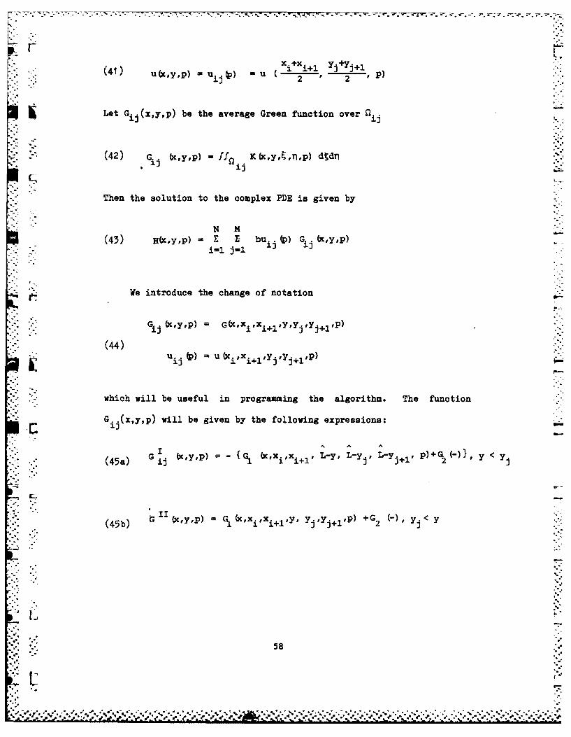
L.+ yj+yj+l(41) u (X,y,p) = uiP) U 2 2 p )
Let G. ij (x,) be the average Green function over i
(42) G. (X,y,p) HO K (,y,En,p) dgdj
L . .ij
Then the solution to the complex PDE is given by
N M(43) H(x,Y,P) = - - bu (p) G (x,y,p)
i-l j=1 ij
We introduce the change of notation
G. (XYP) = (XXi 1.
(44)°.UL ij * ) u (Xi +lYj Yj+l,p)
which will be useful in programming the algorithm. The function
G.j(x,y,p) will be given by the following expressions:13
(45a) ij 1 Y, xiP)i+l ' L-y, L-yj, L-yj+ , p)+ (-1,y < y
G (x,y,p) C7= (Xxi,xi+ly, yj,yj+l,p) +G (,yj < y
(45b) liil' 7 ~ 2j
58
• I.-
-14 V 7
. (45o) G (X,y,p) - G I X ,y-yjry,p ) +G (,xi,xi..lL-Y, L-yj L-Yp)
y. Y< y_.-V " - -j+Il_,
where
2nITX2 si (--- sh Un .-y) Ir., %_1-) .{ 2 Ln~
n7rx n7rx i+-Cos x {ch 4ly.+) -ch (11j)Y
{cS L L n + f
i.'.~ ~ --fntx ,, noV no~ I-.
(46b) G2 - H VIC nI' nj n L -)L- -Co
X 2 2 .-.2 J+n 0(46."b-)x2 % = J l - i ) "'""" %-X~ 1
The computational algorithm based on this representation of the
solution is given in Figure 4.2.
4.4 Eigenfunction expansion of the solution
of the generalized wave equation
In this subsection we shall use an eigenfunction expansion to
solve the system (1) as an evolution system in time. Using the
exponential transformation (2) we can rewrite the system as
*2 22"'" ' '[8_ +b '+dg +bu in a[2i• ~ ~ ~ a a-," x ay.,-
(47)
I., L g-O on g(x,y,t 0 ) go(x'y)' gt ,Y't0)= g9 c,y)
59
. %.- ,.-- .. ..-- .
'. .. . . ....:.,"
Here ve use general boundary conditions since ye want to use the
solution to simulate the response of the membrane system to inputs
based on its state at a given time. Our solution -7 expressed in
terms of an eigenfunction expansion. Let n (x,y) be the
eigenfunctions of the operator in (47) and suppose that the data and
L the control function have the form
u ', ,yt) Z u t) n (x,y)
m,n mn Mn
( 4 8 ) 0 x y t )r O n x y qxg (x'ytO) .. --. .C-y)
* -. m,n 1 m,n
We look for the solution in the form
(49) g (,y,t) M E ( nt) @ 'y)m~mn
This leads to an eigenvalue problem
(o 2 2 mn mn ton
0n~ onM
C and an initial value problem
a (t) C& a_ (t) +b u (t)a .(()) am On mn Ma (o)-=r , a. (o) =v
A simple calculation determines the eigenfunctions
(52) (mn Y) sin (T) sin
corresponding to the eigenvalues .,,_
va5-
() X~ -d- a 2+b pl) ]
60i , -
- . '*'." . .* . . . . . . . .-.

- - . : -
The initial value problem has different solution forms depending
on the sign of X . Let t0 be the initial time and let tf - t0 + T,
where T is the sampling period. WhenX < 0, we have.m b v1 -cos $
CL (t ) r coo 41 T)+ sin(J T)+ * Rnmn f in I mn
WI h nI U h
• ;..
(54a) WIinU. T
When X. 0, we have
T2-(t) r + i' T +b
rn f R UI -an 2
(54b) &l (tf)V + bUWIT
When X > 0, we have
hifl
(54c)1 &(f=JrWsiIT) + vM h (WT) + u sh IMT) -
_ These expressions permit us to solve the membrane system from any
-'. ~initial conditions for any control input satisfying the condition that "
(t". r c-O
it be constant over the area of the mesh element in Figure 4.1.
: * .- ..,
-- U
These exrsiospritu:osov.hemmrnesse fo ninital cndiionsfor ny ontrl inut atisyingthecondtiontha
"e. -1 ".',' " "i t"" " b e-- .c-o-n s t an- t .. o. v er..- .. - .th e, • • a r-e•a -o• •f -t• .h e• • m-e s•h. • •e l• -. ..e-n. .-. ...n F-.i- ,g- -r e ..-4 -,' ...0.• " - " . o "- o.. " . " ,J ' , , '- - -, ' ' ' '
S61: ,',: .', ,.,,: .:._.._. "._. . . .'_' .,'.' ."J ." " • "= ,-'-

*, .4, -.- * -T ,_'l . -. * -. ._
, " * * % ."-w...- . % % * . .. . . *. ".•:. •.",-" • . .*..-.- ... - ..-.-. -... .- .. .- * - .w_- _-
- - ,-
4.5 Spectral factorization using the Hilbert transform
Computation of the optimal stabilizing kain based on the Davis - :
Stenger spectral factorization procedure used for the Euler beam
problem proved to be infeasible in treating the two dimensional
system. The computational effort was too high to be practical; and
it was necessary to redesign the algorithm to achieve greater
numerical efficiency. The key idea was to use the Hilbert transform
"" :'to represent the spectral factors arising in the calculation. This -',
permitted the use of fast and efficient numerical Fourier transform
techniques in the gain computation algorithm.
Given a Fourier pair (fF) in L2 xL-.
(55) fx W L-x (s) ds, F (s) r sXf(x)dx
the Hilbert transform is defined by
____ 2f- (r dr CL(56) m(t) - .-.-d.-
.7! - t-r
where the integral is taken in the Cauchy principal value sense.
Givjen a complex function
(57) T(s) R(s) + iF(s)
then
(58) HT( w) HR( w) + iH}'( w)
k.,,.*
62
%'.~ %,. %- L. . . . . . ... . . .. . .. . . .. .. . . . . . . . :: :
The inverse Fourier transform of HT satisfies
* (59) F_1 fliT) -isgn(t) F-1 fT) __
Ifsw define
T - - r-i E), T- -
(60) +- 1
then .L.
0 t>O 0 > 7'6) -1
(61 C: t'4) 0 0J -.
This means that T +(respectively T ) is the projection of T onto the2 ~2 2
space L+(respectively La with the obvious intepretation of L + and
L.
Nov consider a function f(x) satisfying the condition .7
(62) lim f(x) -1
2if * (x) f(x) -1, then *e L .Applying the previous results to
L; the function
(63) (Fx) l og Ef(x)]I
(with the proper choice for the branch of log), then
(64) f~x W f+(x) f -W
where f+ and f- are the causal and anti-causal spectral factor.,
63

-7 TC -,P -3
respectively. For instance,
(65) f-(x) - f(x) explli Hiog f(z)1
2
This expression is used directly in the computation of the optimal :.
stabilizing feedback gain by spectral factorization. :.:
4.6 Gain computations
In abstract form the control system (1) takes the form
x(t) -Ax + Bu
(66) y(t)- Cx x x().-
The transfer function is . .
(67) G ij)) - CR W-o:A) B
where R(iw ;A) is the resolvent operator
(68) R (iw;A) - W-A-
If we compute the spectral factor of I *G*G
(69) F W3) F (oa- (I+c?G) (1w)
then the gain is given by
64
kt
In the present case the components are
• (71) 3' -- xx~+ W in + d "''
And we shall take
.'-~ 0 , -".
(72) c-i2 2 B.L)
L k 2which allows for weights on both the displacement and the velocity.
The resolvent operator is computed by solving the system
(73)
which leads to the system
+ b - (2-cs) f= (cu-v) -su
(74)
.x..
f=O on W, g-sf-u
The associated transfer function is
(75) Giw W ) .
-k 2 92 OW)•
where I"','
65
," ",- -.. . . . . - .... A , . . I . . . . . . . . . . . . . .. .. _ -
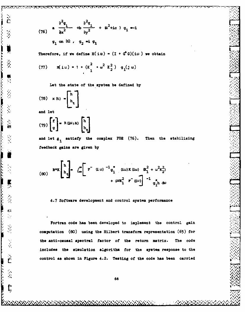
a2 9 2g' 2g 212
Sa - +b - + 2+ic ) g.-(76) 2 2.
gon al g 2 =ig
Therefore, if we define H(iw) - (I + *G)(iw ) we obtain
2 2
(77) (iw) + (K K ) ( ) ,.
Let the state of the system be defined by
(78) x(t) M j
.* and let
.I (79) 9 (JW A)-,-:":''
and let g1 satisfy the complex PDE (76). Then the stabilizing
feedback gains are given by
1~" (i-'"-"
h cF 2(80) ~ ~ - 1) ~ w G 1 w 2
+ W2 - 1
* • 4.7 Software development and control system performance
Fortran code has been developed to implement the control gain
S"computation (80) using the Hilbert transform representation (65) for
S'the anti-causal spectral factor of the return matrix. The code
includes the simulation algorithm for the system response to the
control as shown in Figure 4.2. Testing of the code has been carried
66 : i* ..,,.-

out for a few values of the weights in (72). The results indicate
that the stabilization of the system in significantly enhanced by the
P control action. Since we take the damping in (1) to be positive, the
~ system is stable for small enough bias voltages. Modest values of the
control weights (10 on a normalized scale), produce a 20% improvement
ILL in the settling time of the system. Kxtensive testing will require an
upgrading of the numerical routines in the code to produce faster
solutions of the system.
67
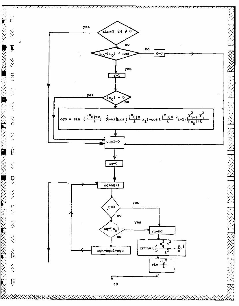
. . . . . . . . . .. . . . . . . . . . . .67-.. . . . . -. - 3 . ---
Iyes
yes n]-no 3,-
2 2
(00
]Tx go(Or(012 }-3J
ego= in( ){cos-x)-os,-n+
nof
La ng n4-~~r. cg-gl
r~i 68
iv3*~3*-3

~cp- (ch (Png y. -ch aing y.) sh 4±ng (-y))/sha 2.)j+-4-.
cgn-crp w cp +cgol
Figure 4.2 Algorithm for control gain computation and simulation
L0
- -~ * - .
Part II:
Effective Parameter Models of Heterogenous Structures
5- -
I2..
*9
5. Homogenization of Regular Structures
It is now generally accepted that large, low mass lattice -
structures, e.g., trusses, are natural for space applications. Their
large aiz'e and& repetitive infrastructure require special techniques
for structural analysis to cope with the large number of degrees of
freedom. As Noor, Anderson, and Greene (1978) point out, continuum .
models provide a simple means for comparing structural characteristics
of lattices with different configurations, and they are effective in
representing macroscopic vibrational modes and structural response due
to temperature and load inputs. Our approach to the construction of
such models is presented in this section. In the next two sections we
consider the problems of control and state estimation in combination
with the construction of continuum models. We shall begin with a few 0
remarks on related work on continuum models in the recent structural
mechanics literature.
Noor, et. al. (1978) use an energy method to derive a continuum
approximation for trusses with triangular cross sections in which the
modal displacements of the truss are related to a linearly varying
displacement field for an equivalent bar. In (Dean and Tauber 1959)
and (Renton 1969), exact analytical expressions for the solutions of.
trusses under load were derived using finite difference calculus. By * **-
expressing the difference operators in terms of Taylor's series Renton
(1970) vas able to derive continuum approximations to the finite
differen~ce equations resulting in expressions for equivalent plate
stiffneuses, for example. In a recent paper Renton (1984) used this
70

approach to give equivalent beam properties for trusses, and this
5 complements the earlier work of Noor, Anderson and Greene (1978) and
Nayfeh and Hefzy (1978). (See also (Anderson 1981).)
In these papers a continuum model is associated with the original
(lattice) structure by averaging the parameters of the lattice over
some natural volume (e.g. of a "cell" of the structure) and
identifying the averaged parameter value (mass density, stress tensor,
etc.) with the corresponding distributed parameter in the continuum
-model. A specific form for the continuum model is postulated at the
* outset of the analysis; e.g., a truss with lattice structure will ber-
approximated by a beam, with the beam dynamical representation assumed
* in advance. While this approach has an appealing directness and
simplicity, it has some problems.
First, it is very easy to construct an example in which the
"approximate model" obtained by averaging the parameters over a cell
1E is not a correct approximation to the system behavior. This is done
in subsection 5.1. Second, the averaging method (averaging the
* parameters over space) does not apply in a straightforward way to
systems with a random structure, since the appropriate averaging
procedure in this case may not be obvious. Third, the method cannot
be naturally imbedded in an optimization procedure; and controls and
state estimates based on the averaged model may not be accurate
reflections of controls and state estimates derived in the course of a
unified optimization - averaging procedure. The method does not
I provide a systematic way of estimating the degree of suboptimality of
controls and state estimates computed from the idealized model.
71
in this work we use a totally different technique called
IM homogenization from the mathematical theory of asymptotic analysis to
approximate the dynamics of structures with a repeating cellular
structure. Homogenization produces the distributed model as a
I L consequence of an asymptotic analysis carried out on a rescaled
version of the physical system model.
*Unlike the averaging method, homogenization can be used in
combination with optimization procedures; and it can yield systematic
estimates for the degree of suboptimality of controls and estimators
derived from idealized models. Results to this effect are given in
Isections 6 and 7. While our results are preliminary, they
nevertheless demonstrate the feasibility of the method; and they
* suggest its potential in the analysis of structures of realistic
complexity.
In this section, we first give an example illustrating some of
SEthe subtleties of homogenization; then we discuss homogenization for
abstract hyperbolic systems; then we illustrate the applications of
-: homogenization theory by deriving a diffusion approximation for the
thermal conductivity of a (random) lattice structure. In the final
* example we derive a homogenized representation for the dynamics of a
lattice structure undergoing transverse deflections. We show that the
behavior of the lattice is well approximated by the Timenshenko beam
equation; and we show that this equation arises naturally as the
limit of the lattice dynamics when the density of the lattice
structure goes to infinity in a well defined way. The mathematical
analysis used in the derivations is based on the book (Bensoussan,
72
* --.
Lions, and Papanicolaou 1978) and the paper (Kunnemann 1983)."
5,l A one-dimensional example
*" From (Bensoussan, Lions and Papanicolaou 1978) we have the
following example:
d e duo(x- ) =f () x C x 1):.
u- (X (0 u (X
where a(y) is periodic with period YO, a(y) > c > 0, and a'(x) -
a(y/e). It is simple to show that
(2 e1
CX W C (x12 + .4 (x), 2 c .-1_
-.,:c(2) H u I A f u dI <u --a
and so, u -u weakly in the space'HL• Moreover,
(3) ac M (a0f a(y) dy
YO 0
E and it is natural to suppose that ue u with the limit defined by
M (a) d )] - f(x) x C CXo 0 '1)(4) - dx
u(X ) -0 u (x )"' 1.,- .-
This is untrue in general (Bensoussan, Lions and Papanicolaou
*We are grateful to Professor George Papanicolaou for bringing
Kunnemann's paper to our attention.
73
.. I. " ~ *% ****.7 :~ I.. : '" 4

~ -...........
1978, pp. 8-10). The correct limit is given by
( -" C [ u)] f6), XC¢co x ), u (xO) -0- u (x1)
.. ' , - . -with u (X) mOuuc L
(6) a -
In general, 1(a) > a; and so, the error is identifying the limit, (4)
. versus (5), is fundamental.
The system (4) corresponds to averaging the parameter a (x) over
a natural cell; a procedure similar to that used in (Noor, Anderson
and Greene 1978), (Nayfeh and Hefzy 1978) and (Aswani 1982) to define
continuum models for lattice structures. As (5) shows, the actual
averaging process can be more subtle than one might expect, even for
simple problems. :. -
To see how (5) arises, let
(7) F,,),,e ( x) u-a, Wi 4' 'e'dx
Then :(x) is bounded in L2 (xoxl) and it satisfies
dxx-( d , (x)-f (x,), x e (Xo,xl )
One can show that e (x) has a strong limitg (x) in so
,o £..-a
7:. (9) e a-:,-Sa~
*weakly in I? (x x) But,.." ... ,,%y.*, ,, . t"""
"'7* -. ,. -
, ,. ...8,,*
- --: . > - ..." .''.<_"". .... ,0 1...-..:'..' ""
%T'
duu
S(11) =
dx
i ~ ~and since ,"
(12 d&; f
we have .
d "( M( 1 -1 du(13) 3i a ..
and the limit uc* u is weak in H1(x,x2 (the Hilbert space with norm
defined by (2)).
This example illustrates the pitfalls associated with simplistic
averaging procedures.
5.2 Homogenization of Wave Equations
As shown in Part I of this report, hyperbolic (wave) equations
are the most natural models for the dynamics of flexible structures.
General techniques for homogenization of wave equations are available
(Bensoussan, Lions and Papanicolaou 1978). The precise form of the
homogenization procedure depends on the scaling of the physical model;
i.e., the dependence of the system characteristic features on small
parameters. Since this is a sensitive modeling issue, we shall ""
discuss it in some detail. It may be necessary to consider several
scalings to determine the one most suitable for a given class of
75
. . ..*** .'% . .* .- . . . . . . . . . . . . . .'. ,
flexible structures.
Consider the Klein-Gordon equation
". tX) (x) Vu(t,x)] -3(x) u(t,x)tt
(14)u (,X)-f (k) u (ot)-9 (x), t>o, xc
t
where f and g are smooth functions of compact support, c2 (x) > 0 and
W(x) > 0 are smooth. Suppose c(x), W(x), f(x), and g(x) depend on a
small parameter e > 0. For example, suppose c and W vary slowly with
X, so we have°2.2
( ) c- 2 (E x), W-W (C x)
and suppose
(16) f fE g g g'
Let u be the solution of (14) with (15) (16). The behavior of u as
14 't0 in (14)-(16) is trivial if we consider (t,x) fixed. However, if
(t,x) become large as C *0, then an interesting limiting behavior
emerges (Bensoussan, Lions and Papanicolaou 1978, Chapter 4).
To see this most clearly, it is necessary to rescale t and x as
(17) t = ,
Dropping the primes, this yields
C2 C(t': X)-' -V (tx"'C2WVu ltIXl W) Ju IX./ "-. tt 2 tx "" ....
(18) -• u (o'x)-f , ut ; X- Rn, t >o0 ..
..
Notice that in rescaling a system with slowly varying coefficients,
* 76-e- . . *

-7l 47 W I 7
A. -.
one produces a system with a large coefficients.
To complete the specification of the problem it is necessary to -
define the dependence of the data f E and g e on d . The various choices
strongly influence the final form of the limiting system. Following
[ (Bensoussan et al. 1978), we shall distinguish three classes of data.
,A Case 1: Low frequency problem
*][ In this case fe and gC have asymptotic power series expansions
( 1 9 ) f (X ) N f0 W'g (X) ^ gO W + C .'. . 1-.-,
where the terms in the expansion are smooth functions. To produce a
problem with finite energy as C .0, it is necessary to take fo(x) = 0
in (19). (See (Bensoussan et al. 1978 p- 541).) Since the problem
is linear, it is not necessary to have the expansions begin with t
The analysis of this problem is comparatively simple, and the
limiting behavior as co 0 is elementary.
Case 2: High frequency wave propagation in a slowly varying medium
In this case th9 data take the apparently specialized form• =,
,".-'-"
o:f¢ W N" exp 0 1 s (x) / I f€ Wx :.
(20) , x.'i .)'9 (X - exp is (X) /C g¢ (x)
,* _.-,
77
NOWet
""
where S() is real-valued and smooth, and and e are complex-valued
and smooth and have asymptotic expansions like (19). Note that the
data in (20) are complex-valued. Since the problem (18) is linear,
*both the real and imaginary parts of u are solutions.
To understand the physical significance of the second case, k
suppose the "phase function" S(x) - k x, where k is a constant vector
V- and dot stands for the inner product in R2 . In this instance the data
in (20) are spatially modulated plane waves with rapidly varying
phase. As shown in (Bensoussan et al. 1978) virtually all cases of
interest (different scalings leading to nontrivial limiting behavior)
can be analyzed in terms of this case. For instance it is possible to
treat the case of wave propagation in slowly varying media with -"*
i spatially localized data or the form
l-n/2
f"(x) - f(x, )
(21)g. W -n/2 x . - .
where f and g are smooth functions of compact support in x and y
."(x/), and (x,y) £R2 . The scaling on the right in (21) is chosen
so that the terms are of order one as e+ 0. Problems with forcing
functions and/or inhomogenous boundary conditions can also be treated
by essentially the same method. "-.
The treatment of case 2 given - (Bensoussan et al. 1978) is'. ,---
based on the ideas of geometric opt -,. The solution uE is sought in
the form
C, 78
%' ;. : :. 0 . * .* .*. .a . a a .•
.... .. . . . . . .- "-*- , -.
u~ (x,t0 e iS Xt v (X, t)
(22)v (X, t) -v 0 (X, t) +ev1 (X, t) +..
Inserting (22) into (18) and equating coefficients of equal powers of
C leads to
(23) 1 V1 A 0
A v +Av 0Av-(2) 121 21 30
where 2 2 2Al -c (VS + (S ) -
2 2A n2 i S (VC a) + ic V S V iS
2 t t
(24)22
A 3 V (C V)-a3
The analysis of these equations leads to the reduced model for the
system behavior.
From the first expression in (23) we see that for v0 not to be0
identically zero ye must have
(25) S- (c 2() S 2+ 1/2 0
This is the eikonal (or Hamilton-Jacobi) equation, a nonlinear first
order PDE which controls the evolution of the phase function. It may
* * ~*be solved in terms of a system of nonlinear ODE's (Hamilton's
equations) for the "rays" and "momenta" associated with the
propagation of energy by the system. (See (Bensoussan et al. 1978,
79
.p77
'U * ~ ~ ~ ~ * K A .* . .. ~*;~~* ~ . >- - ..
The choice (25) for the phase makes the operator A, identically ,.
zero. Using this in the second equation in (3) leads to the
"transport equation"
(26) A2 v0 -0
Its analysis leads to expressions for the propagation of energy in the
system. L
The case of spatially localized data (21) may be treated using
the same techniques in combination with the method of multiple scales.
. e shall not develop the analysis of these general systems in more
detail. Rather, we shall turn our attention to the construction of
continuum models for lattice structures.
5.-3 Continuum approximations for lattice structures ,,.
In this section we shall apply homogenization and the associated
S"asymptotic analysis to derive continuum approximations for two
different types of problems. In the first case we show that the
problem of thermal energy conduction in a lattice can be well
approximated by a diffusion process in the macroscopic scale. In the
, second case we show that the in-plane macroscopic (2 dimensional)
motions of a simplified truss model can be well approximated by the
Timoshenko beam system.
-" 80
-,~..% . . 4 . 0 *--.* -:..0.. . ,, 4

5.3.1 Effective conductivity of a periodic lattice
A. Problem definition
* " Let Z - 10,+1,+2,..o) and - Z x...x Z (d times) be a
d-dimensional lattice. Let C >0 be a number small relative to 1. We
want to describe the effective conduction of thermal energy on the
-- spaced lattice C . Let ei - (0,...0,i,0,...0) with I in the ith
position, i - 1,2,...,d. If x is a point in Zd, then x + Ce1 ,
I < i< d, are the nearest neighbors of x. Let ai+(x) x zd
1 < i < d, be the two functions defined on the lattice, and assume
(26a) a.c):-a (x) =a (x+ei) x £ zd, 1 i < d•. ... ai ai+ : i
d < <(26b) 0 < A a. (k) - B < x C Z , 1 = i = d
(26c) *a (x) is periodic with period 2, > 1 in each direction,*
1 < i < d.
Next let
(27) a (x) ai x/) xEcZd 1 i 9 d
Equation (26b) means that the conduction process is reversible
and that the conductivity a( x) is a "bond conductivity", i.e.,
independent of the direction in which the bond (x,x + ei) is used by
the process.' Equation (27) means that the configuration of bondconductivities a* .) one . is simply ai+() on Zd "viewed from a
L distance." Assumption (26c) imposes a regularity condition on the
*The period may be different in different directions.
81

physics of the conduction process. An assumption like this is
essential for existence of a limit as e 0. In one dimension the
situation is illustrated in Figure 5.1. A system similar to this was
treated by KUnnemann, (1983) with random bond conductivities.-*..
Ergodicity replaced periodicity in (Kunnemann 1983).
A
Figure 5.l.a. Conductivity on unscaled lattice with period L6
/~ 7f%-
N0.-
Figure 5.1.b,. Conductivity on e-scaled lattice, y e x, with
x e Z and period c2s 6
One can associate with this system a random (jump) process
Ix t~),t > 0, xe CZ Ion the E-spaced lattice*. In effect, as
C -; 0, XC converges to a Brownian motion on the lattice; and the q
main result of the analysis is an expression for the diffusion matrix .
*Definition of this process is not necessary for the analysis, but it
bolsters the intuition.
82
e& I ft t. . . . . * * ttft tf f t.f
Q: i[q i ,j - 1,2,...,d] of this process. This matrix describes
the macroscopic diffusion of thermal energy in the system. It is the
effective conductivity.
We shall carry out the asymptotic analysis of this system in the
limit as C-1O using the theory of homogenization. Let
(Viu) (x): - Eu (x-Ce)-u (x)]
(28) +( U) (x: uZd e)-~~
X.Z , 1 S d,
for any u square summable on Z or square integrable on Rd with e
dthe ith natural basis vector in R . Then
au (tx) md -- C ( tx)V-[ V e@) V. u (')
at. i C I*-" (29) i--
--L U (t,x)
is the diffusion equation on the E-spaced lattice with density u(x)
and conductivity a1 (x/e). Our construction of an effective parameter
representation of the thermal conduction process as e + 0 will be
based on an asymptotic analysis of (29) using the methods in
(Bensoussan et al. 1978).
-, .' Remark: Although we shall not use probablistic methods in the
-- analysis, the associated probabilistic problem has a great deal of
intuitive appeal. The operator L e may be identified as the
infinitesimal generator of a pure jump process X£(s) in the "slow"L time scale a: E t; cf. (Breiman 1968). Moreover, L is
83.T " "Z-'

dselfadjoint on Z with the inner product
' ": (f~V') •" £ (f W lg Wx ';(30) xczdf").E
Hence, the backwards and forwards equations for the process X (s) are,
respectively,
Eap (Ytlx) - Cp£(yutI-]Ix)at -
3)(31)
-p (y,tlx), -[L£p (.,tlx)](y)at
So the process is "symmetric" in the sense of Markov processes
(Breiman 1968).
The asymptotic analysis of (29), when interpreted in this
context, means that as the bond lattice is contracted by e and time is
sped up by C , the jump process Ixe(s)} approaches a diffusion
process with diffusion matrix Q. In other words, on the microscopic
scale thermal energy is transmitted through the lattice by a jump
process; but when viewed on a macroscopic scale the energy appears to
diffuse throughout the lattice. The microscopic physics are described
. in (Kirkpatrick 1973) and (Kittel 1976).
Because the basic problem (29) is "parabolic", we can introduce
the probabilistic mechanism and make use of it in the analysis. In
the "hyperbolic" problems we treat later, this device is not
. available.
84
rTB. Asymptotic analysis-homtgenization
The essential mathematical step is to show strong convergence of
3 the semigroup of L say
(3"T (t):exp(L t)i (32)
Tit M=exp'lMt)
and identify the limiting operator
d a2i .-.- (33) L- Z. Mi x x... i,j l i
This is accomplished by proving convergence of the resolvents
(34) for a > o, [-L.E +a] - -L+a]-l
That is, if f is a given function and
£ E -
U (.):=[-L+at] f
(.):-[-L+zl 1f
then u u (in some sense).
The method of multiple scales developed in (Bensoussan et al.
1978) will be used to prove the limit. Because the conductivities
a (x) in (29) do not depend on time, we may work directly with L[ " irather than the parabolic PDE (3) (cf. (Bensoussan et al. 1978
Remark 1.6, p. 242). The method of multiple scales is convenient
because it is a systematic way of arriving at the "right answers" -
something which is not always simple in this analysis.
85
L%
AD-RI5B 736 MODELING AND CONTROL OF LARGE FLEXIBLE STRUCTURES(U) 2/2SYSTEMS ENGINEERING FOR POWlER INC ANNANDALE YRB1 MR8YRAMOYIC ET AL. 31 JUL 84 SEPI-TR-84-9 N
UNCLAISSIFIED RFOSR-TR-85-0075 F4962e-83-C-ei59 F/G 12/1i NiInhhhhhhhhhhI fflffl|lfll|fflfflfI lfflffllfllIlfllfIIIIIIIIIIIIIIIIIIIIIIIIIIIIIIIIIIIIfllfllfllfllflIIIIIIIIIIhm

J.,~
11111 11.631
M RI
i1ROCOPY RSUIO TES CARNATONA BREA O SAD193 -A
~~%%~11 1.1e C

oJFollowing (Bensoussan et al. 1978) and bearing in mind (35), we
consider
(36) (LCu) (x)-fW(x)
with boundary conditions to be specified later. We shall look for u
in the form
(3)u £ xA C (xM 2 NAh+.0 CC 2__
i:":(37) u (xlmuolx.E)+CUl """)+- 2" "
d .-with the functions u (x,y) periodic in y c Z for every j O, ,,....
(As it turns out the boundary conditions are somewhat irrelevant to
the construction of "right answers.") To present the computations in a
simple form, it is convenient to introduce y - x/c, to treat x and y
as independent variables, and to replace y by x/c at the end.
Recall the operators V from (29). Applied to a smooth
function u -u(x,x/e), we have
." -£u) tx,y) U u(x-ce i , Y-ei-u c,Y).
(u (y-e i) -u y)]
1:-1 l u) y-) -u +,-e) v'- '.. : + [u (x- e., y--.."~y-
1 2.u a u ('-2"+.
where on functions 0- 0(y).
86

,, . - - -*-. - - - S - - R -J . -r . o.
Defining
S(40) (V -"" y+ei) - *( :(Y)
S:-:, we also have '
1 +V)(xVI, (u ) (e.j2u(XY+y ) +0 L ...
(41) (V u(x,y) x ( X 3x (xy+ei) + 01 (
Now we substitute (37) into (36) and use the rules (39) (40).
Equating coefficients of like powers of c, this leads to a sequence of
equations for U, u ,... Specifically, (using the summation0 1
' 'convention)
"u) (X,y) - -V i V1 i
i iu-V C [ a au 0 ,y+e )]
1 2o
(42) i - cV i [a. ( ) -- ,y+e) +0(C)
. !V [a kfy) V u CY)"
au- 1
u x iY)] +0 ) f(X
That is, labelling each term by its order in ,
(f,)( V, V7ai(y)V+ u03 0'- -"(43) i,0; -
. 44 £- [ai (y) L2 (x,y+e )]+V (a (y)v u (x
- and (recall V t+- 0(1) in c)
87
L.

.2u: i (a fly) jx. (X'y+e,)]
0 e,2 au :;(45) o (xy+e )]
S - - a ) V+ u2 KY)] f (x)
From (43) we have w
a. (y-e u (x,y) - u (y-e ) ".
(46)
-ai (Y) [u (xy+ei) -u 0 0,y) m L
If we take u0(x,y) uO(x), this is trivially true. (We must justify
this choice in subsequent steps') And (44) simplifies to
(Y - + % (X,' ") 0 '-
(47) £V a (y) - (x) ] +V. [ai(Y) V -'."a
£At this point we invoke a standard device in homogenization asymptotic
analysis, namely, the use of "correctors." We assume %'d aul
0(48) Ul(X,y) m Xk(Y) . + u(X)u"(48) U
k-1 kwith xk() the correctors. Using this in (47), we have (agair
using the summation convention)
- au ° a u o- + 0~Y) 0~~1(a:i -- V ( + [ak (y - ek )- ak (y )]
(49) Vi (ai(y) V. Xk( ON +x k k.k-.0
O~"- 'k.'
If we take Xk(Y) as the solution ofk+
(50) V1 [a1 (Y) V×Xk(Y()] + [a (y-ek) -:.... 'C.. .- ..
',- (we have to verify the vell-posedness of (50)), then (49) is£Isatisfied. (The term () is determined (formally) from the 0(C)
88
* C C *C*C
• ". "' ' ' " "" '. '.,- '.- _ ., "'::, i. , . - - .. ... ,.-.- -- ..- -. ,'. .> -- ,%,%*

4'' term in the system (37) (42).) .
Regarding the well-posedness of (50), note that
(s) Vi-[ai(y) V. f(Y) I T ' (Y)
has a periodic solution onEZd which is unique up to an additive
constant if the average of the function '(y) over a period (ei) is,I..';.
zero; i.e.,
-: (52) Z " - (y+k )- 0 n-1, 2;,... dIk-I
* r' This condition clearly holds in-'(50), and so, Xk(Y) is well defined
(up to an additive constant).
We shall determine the equation for uo(X) by using (48) (50) in
(45). Using the Xronecker delta function 6 ik9 we have•ai ' ) Sik'
*: . a x a x : ' V
axiaxk
-, =~~~{ Vi - [ ai )6ikJ -Vi - [ ai 1 Vi+t Xk] } ai ...
.-V1.- ai () x ky)] 2 - -fa (y)V *u ]
i k i i 2The term in braces is zero from (50). To obtain the solvability
condition (52) for u2 in (53), we introduce the average
(54) qik symmetric part ( { -Vx a)2ii i~ k
Then solvability of (53) for u2 gives the equation
89
.. ... .. . .. . .. , , , . .. .. .. . ., .. . . -,
a~m - ~.. -
* (55) q 0Ai 3x "- f (x) "..
ik-1
And this is the diffusion equation which defines the limiting behavior
of the system (36) in the macroscopic x-scale in the limit as+0..
We can justify the asymptotic analysis by using energy estimates
or probabilistic methods as in (Bensoussan et al. 1978). (See also
Kunnemann 1983).) We shall omit this analysis here.
:* S C. Summary
Returning to the original problem (3O) for the evolution of
• .thermal energy on a microscopic scale, we have shown that the thermal
density u(t,x)*u u (t,x) as C+ 0 (in an appropriate norm) where
d 2(56) aU0 a 0
t 2 ~ q1 x xati,j-1 ax a
with
j * [a. (a 1.Y) l(s7) .- - k- l
+Vk [a ak f)X(
.and the correctorsXk, k i 2,...,d, are given by
[ .i ( VY) aXk ain' (] ck) 'ak (-Y)
.. (58) --k_ 1,2,...
To compute the limiting homogenied model (56), one must solve the ...
system (58) (numerically) and then evaluate the average (57).
90
777 -
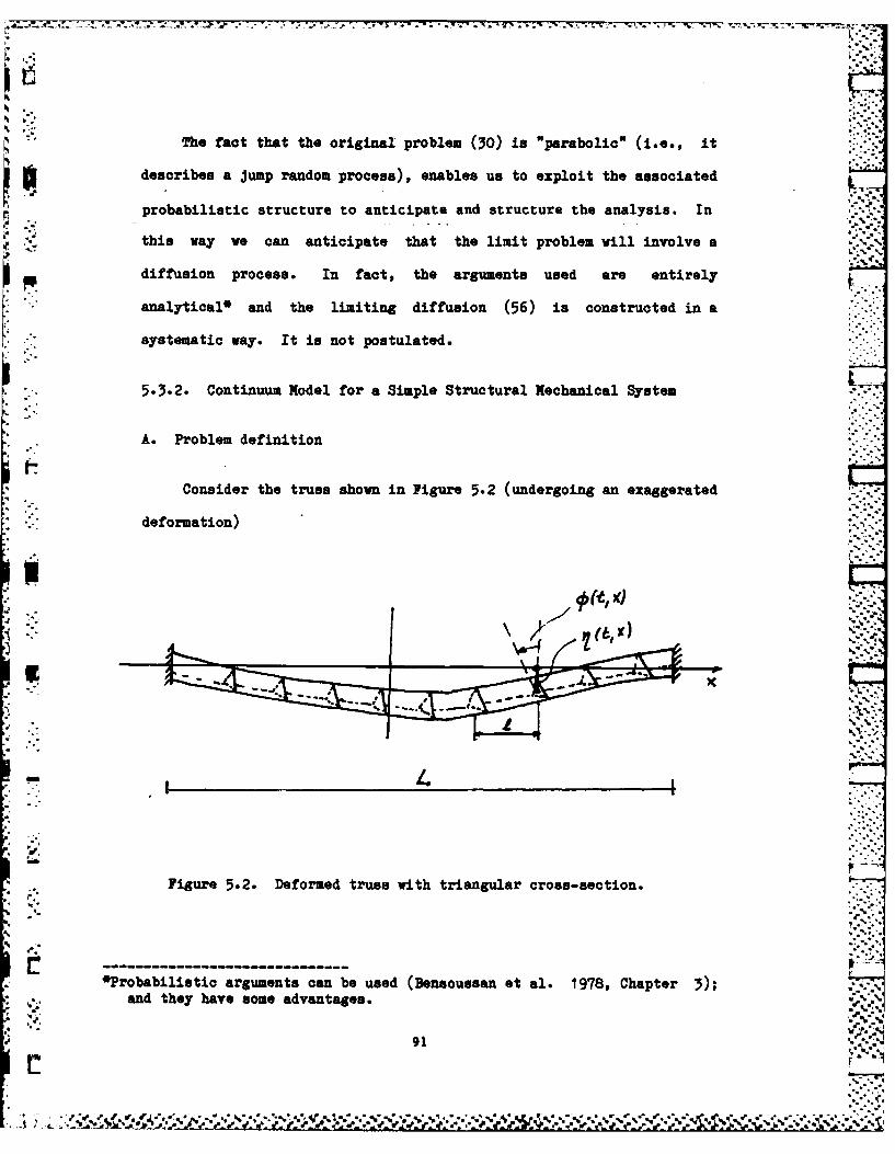
The fact that the original problem (30) is "parabolic" (i.e., it
describes a jump random process), enables us to exploit the associated
probabilistic structure to anticipate and structure the analysis. In
- this way we can anticipate that the limit problem will involve a
diffusion process. In fact, the arguments used are entirely
analytical* and the limiting diffusion (56) is constructed in a
systematic way. It is not postulated.
5.-3.2. Continuum Model for a Simple Structural Mechanical System -
A. Problem definition
Consider the truss shown in Figure 5.2 (undergoing an exaggerated
* -. deformation)
_ . :.:: .. :
Figure 52. Deformed truss with triangular cross-section...
robFabiuitrc argumentscan 5.2 be ous withrssan et l. 1978, Chapter );
* a'.'and they have some advantages.
• ' 91 ..
. ~ -- - ~ -. .-.---
We shall assume that the truss has a regular (e.g., triangular)
m U cross-section and no "interlacing" supports. We assume that the
displacements of the system are "small" in the sense that no
components in the system buckle. We are interested in describing the
dynamical behavior of the system when the number of cells (a unit
between two (triangular) cross sections) is large; that is, in the
limit as
(59) 0-= ,/L * o
We shall make several assumptions to simplify the analysis.
First, we shall assume that the triangular sections are essentially
rigid, and that all mobility of the system derives from the
flexibility of the members connecting the triangular components.
Second, we shall ignore damping and frictional effects in the system.
Third, we shall confine attention to small transverse displacements
n(t,x) and small in plane rotations V(t,x) as indicated in Figure 5.2.
We shall ignore longitudinal and out of plane motions and torsional
twisting. Fourth, we shall assume that the mass of the triangular
* cross members dominates the mass of the interconnecting links.
Systems of this type have been considered in several papers
including (Noor et al. 1978) (Nayfeh and Hefzy 1978) (Anderson 1981)
and (Renton 1984). In those papers a continuum beam model was
hypothesized and effective values for the continuum system parameters
were computed by averaging the associated parameters of the discrete
system over appropriate cell volumes or areas. Our approach to the
LL
i.': "" problem is based on homogenization-asymptotic analysis and is quite ...
492
4 . "" ..

different from the methods used in these paper.
pThe assumptions made above simplify the problem substantially. 7
By assuming the cross sectional components to be rigid and ignoring
out of plane, longitudinal and torsional motions, we have effectively
eliminated the geometric structure of the truss. We can retain this
structure by writing dynamical equation. for the nodal displacements
'] of the truss members. For triangular cross sections nine parameters
describe the displacements of each sectional element. The analysis
which follows may be carried over to this case, but the algebraic
complexity prevents a clear presentation of the main ideas. As
suggested in (Noor et al. 1978) one would need a symbolic
manipulation program like MACSYNk to carry out the complete details of
the calculations. We shall take up this problem on another occasion;
'for now we shall treat the highly simplified problem which, as we
shall see, leads to the one dimensional Timoshenko beam (and from
there, under certain constraints on the parameters, to the Rayleigh"I,- and Euler beam models).
We shall begin by reformulating the system in terms of a discrete .,.
element model as suggested in (Crandal et al. 1980); see Figure 5.3.
In this model we follow the displacement T(t) and rotation *,(t)
of the ith mass N. The bending springs (I ) tend to keep the system
straight by keeping the masses parallel and the shearing (k!) tend to
keep the masses perpendicular to the connecting links. We assume
small displacements and rotations so the approximations
93

'Ir
Figrure 5.3 A lunped parameter model of the sinplified truss system.
sin (t)
1/
(60)tan (hl C t) P. Z n W)/
are valid.
In this case the (approximate) equations of motion of the ith
mass are
~L ~ 5 ~ i+l MM k'
S "
(The spring constants depend on a since they represent the restorative
forces of flexed bars, bend by different amounts.)
94 . , ..-
sin I S (41•.".
" M -t + (t)(61b) t) - I { YO ]-
where we have normalized a 1 and defined
(62) Sn- i
and similarly for (We shall omit trwa :er:, of the boundary
conditions at the ends of the system.)
To proceed, we shall introduce the nondimensional variable C = t/L
and rewrite the system (61) as
M) fVcn (t) - o*i (t) +V1+ {V mV""r 8 .
(63) T i(t) = - -{K Vn.t)- A i t ) )1 M M1
where K.'.'i-
- k L, X k
-. . (64)+ 1-. :::.:. _V Ci = (ni+1 - ni ) , V ni (ni_ i-l) -:"'
Next we associate a position in the system xiC-1/2, 1/2]
. (normalizing L 1 1) with each mass; and we introduce the -notation
(65) l(t,x.) = n( t), *(t,x.) = Mt)
Having normalized L 1 , we have e-I and xi -x. - x. + e.
Let - }x be the set of all points in the system. In this notation
95
.. -~~ ::->~~.'.-."
6. .7-
(66) (t, x) - (r[(t,x+) - r(t,x)]" ~( 6 6 ) : ' L -
1 C"'.'- "A
- . (V r') (t,X) - [(t,x) - f(t,x-C)] , xC Z
* '. 2and the system is
"e(tx F.. (x.){V£+-C(tx) - (tx i .
.(67) +V+]
Ti (tx) - VV£K S(x.)[V C+TiC(t,x) (t,x)IW
The scaling of (67) may be interpreted in the following way:
Formally, at least, the right sides of both terms in (67) are 0(C2).
" -This implies that the time variations are taking place in the "fast
time scale" T - t/C. Also, the spatial variations are taking place in
the microscopic scale" x which varies in C-increments (e.g., xi+1 - xi
+ C ). Introducing the macroscopic scale z - Cx, and the slow time
scale a -CT , we may rescale (67) and observe its dynamical evolution
on the large space-time scale on which macroscopic events (e.g.,
"distributed phenomena") take pl.ace.
Rewritten in this spatial scale, the system becomes
7. C Y2,lZ ) i Z.U-
dt 2 C S C-'
(68a) Zi"" - (C - }+""
2C Ci z.
..d T'-(t
+ c- C-L(68b) C _ 1k z 6~c(~' cc(~2 2 CC {C( 6 ~ Ct- C t-]dt
96
-' - *" . bY. h t R K 9 a % ok>~
where
C + C+(69) 6 = V -o(1) in e
The essential mathematical problem is to analyze the solutions
IP, flof (68) in the limit as e+0.
' B. Mathematical analysis
To proceed, we shall generalize the problem (68) slightly by
allowing K and K to depend on z.as well as z/. This permits thes b
restoring forces in the model system to depend on the large scale
shape of the structure as well as on local deformations. We use the
method of multiple scales; that is, we look for solutions of (10) in
the form
.. :: fl:(t) = T(t,z,y) YZ/L
and we have
*(7) K=K (Z,y), Kb K(z Y)u y z• (71) Ks s ".j
On smooth functions P(zi ) the operators satisfy
(6 1p) (Z,y) - 1P (Z+E;y+1) -* (Z,Y)
=.4. (z,y+l) - P (z,y) + 4' (z+e, y+l) - 4' (z,y+l).(72a) 1(Y) +C (zy+l) + (z,y+l) + 0 ( 3)
az2 2
2 --. 9-
,...o o;.* * **-. . -..-... . . .'.o ... '. . ... ,..-....,. ,,.........,.. . .' '.., - .- - - - - -

r° (6 E- ' ) (z,y) - 4 (z,y) - 4 (z-C,y-l) .
N(72b) - 4 zY) - (z,y-l) + (Z,y-l) -AP (Z-,y-"
. ... = - ) ( ,y ) - (z , y - l ) + 2 (Z , y -1 ) + 0 (E.
We assume that , Ti may be represented as
4' (t,z,y) - ' 0 (t,z) + 1 (t,z,y)+...
(73)n (t,z,y) - no (t,z) + E nI (t,z,y) +...
and substituting (73) in (68) and using (71) (72), we arrive at a
sequence of equations for (V nl )', ('l, ' by equating the
coefficients of like powers of e.r
-~-1 0Starting with £-, - 0 '.we have
-(74) r K(z,y) S 0 (t,z)] = 0
which is trivially true from (72b) (73). The same term for (68b) is
trivially satisfied by the assumption (73). Continuing
.1[ r K (z,y) S lI (t,z,y)1 + K (Z,y) {Sn (t,z) -'0 (t,z) }]=0*(75) b (S 0 r
S-which may be solved by using the corrector X (z,y) and taking
T (76) 'l (t,z,y)= x (Zy) o (t,:Z)
with
(77) (z,y) SX (z,y)J K (z,y)
If we regard s as a parameter in (77), then there exists a solution
98

X- -f7 - ----V -7 1; - Z -. . .
XO unique up to an additive constant, if K(,), K(z,-) are
periodic in y, if there exist constants A,B so that
(78) 0 <A < Kb(z y)<B<
and if the average of X (z,.) is zero
(7 1 .2 K (,y) dy-OL() -L/2 S
which holds if the system is pinned at the ends as indicated in Figure
5.3. Let us assume that (78) (79) hold, and
(80) 0 < A < K (z,gy) < B <
(which we shall need shortly).
Considering (68b), the 0(e-1) term in the asymptotic expansion is
(81) [s{K (z,Y) (S n (t,z,y) (t,z))}] -0
Again we introduce the corrector X(s,y), and take in the form
(82) n- (tz,y)- (z,y)0 0t,z)
which gives the equation for the corrector
(83) S { (z,y) IS+X, (zy) -1 -0
or
+(84) s{ '(z,y) s X-(z {.,y)} K (Z,y) -Ks (z,Y-l)
By hypothesis the right side in (84) is periodic in y and has zero
99 t- "'
average (79). Hence, (84) has a periodic solution, unique to an
additive constant.
Continuing, the 0(cO) term in (68a) is
S + {r ]Kb (z'y) S '2 (tr,,y),
+Ks (z,y) ts n (t,z,y) *1 (t,z,y) I0
+K (z,y) (t, Z)
... +S+ {r Kb (z'y) , -1P (tz'y)})'
(85) +s+ {r Kb (zY) (t,z)}2 V'oaz
az:. : +-(rir ,(zy+1)}-'o(,z)3Z a: 2
0 0a!2 r t(z'y+l)} (t at2 a
2. -. This should be regarded as an equation for 1P as a function of y with
(t,z) as parameters. In this sense the solvability condition is as
:- before, the average of the sum of all terms on the left in (85),
except the first, should be zero. We must choose 4) so that this in
fact occurs; and that defines the limiting system.
Using the correctors (76) (82), we must have
s( S+ --Average { (z,y)+- b (s,y) (z,y)i-1. .-. y) i~ 2 i~ 2 ,.-?
-. Bs+at2 a 2 S -
(8E) 0o (r Kb (zy+l))] a 0 K (z ,Y)
"(z y)y LS
+ K & n (z,y) - x (z,y)ll - o ""0
: ~Defining the functions EI(z), G(z) by the associated averages in (86),
100

NT--
* the averaged equation is
(87) - - z . -)+ az HOJ0
which is the angular component of the Timoshenko beam system (Crandall
et al. 1980 p. 348).
Arguing in a similar fashion, we can derive the equation for the
displacement n (t,z) in the Timoshenko beam system -0(
2 3(a.)..2 i 1 3n %,"
2(88) !2no L (z) ( -0 (t,z))
C. Summary
We have shown that a simplified model of the dynamics of the Etruss with rigid cross sectional area may be well approximated by the
Timoshenko beam model in the limit as the number of cells (%L/L)
becomes large. The continuum beam model emerges naturally in the
analysis, as a consequence of the periodicity and the scaling. ',
r° .
To compute the approximate continuum model, one must solve (77)
and (84) (numerically) for the correctors and then compute the
parameters in (87) (88) by numerically averaging the quantities in
(86) (and its analog for (68b)) which involve the correctors and the
data of the problem.
'°- .** 44
101

Ii
. '6. Homogenization and Optimal Stochastic Control
In this section and the next ws show that the process of deriving
effective "continuum" approximations to complex systems may be
developed in the context of optimal control and state estimation -*
- ; designs for those systems. This procedure is more effective than the
procedure of first deriving homogeneous/continuum approximations for
. the structure, designing a control or signal processing algorithm for
* the idealized model, and then adapting the algorithm to the physical
- model. In fact, separation of optimization and asymptotic analysis
can lead to incorrect algorithms or approximations, particularly in
control problems where nonlinear analysis (e.g., of the Bellman
dynamic programming equation) is required. The problems treated here
" "and in the following section are abstract systems which illustrate the
basic techniques. At the beginning of section 7 we shall present a
simple argument which shows how the class of models treated here might
arise. In subsequent work we shall apply the combined homogenization
- optimization procedure described here to the problem of controlling
S"-. the dynamics of lattice structures like the truss structure analyzed
" -in the previous section.
6.1 A Prototype Problem
The interaction of homogenization and stochastic control was
discussed briefly in the book (Bensoussan, Lions and Paponicolaou
1978), and in (Bensoussan 1979) and (Blankenship 1979). The recent
paper (Bensoussan, Boccardo and Murat 1984)* provides the first
systematic analysis of an abstract control problem involving
L homogenization. We shall briefly summarize its main results against
L102
.. ..- the background of the lattice system discussed in section 5.
The problem is to control x (t) given by
dx g X , X ,v) +-bx (% x), dt + G~ ,- 1 dwFt
x(0) mX, 0<t
with x e( t) defined in a bounded domain 0 C R with smooth boundary.
K:Here g, b, and a are smooth functions of their arguments, w(t) is a
standard Rn - valued Wiener process, v is the control and c> 0 is a
parameter. We assume that g, b, and a are periodic in their second
* argument with period one on the unit torus ' in R
e- -Let T be the first exit time ofi C t) from the domain 0. The
cost function is
(v(1) - Ed ( f ~~d L(,e, 1 x ,v) exp -fc(1,- vd)dt
and we define
Cu (x) -inf J (v(*))
V (1
We assume that the cost rate L~x,yv) is periodic in y on the torus,
and has linear growth in v. The discount factor c(x,y,v) is uniformly
bounded, positive, and periodic in y. The set of admissible controls
U adconsists of feedback funct-ions v(-)
£ 1C
[ We are grateful to Professor A. Bensoussan for transmitting apreprint of this paper to us.
103
(Ve shall justify this presumed structure for the control law in more
detail later.) The system has highly oscillatory coefficients; and,
as in section 5, one would expect the solutions of the control problem
to be well, approximated by the corresponding control problem with
4 ;. g(x,y,v), b(x,y), o(xy), L(xy,v), and c(x,y,v) replaced by their
averages (appropriately defined) over y. This is not precisely the
case and one must carry through a complete asymptotic analysis to
determine the exact nature of the limit and the approximation. -
In (Bensoussan, Boccardo, and Murat 1984) this analysis was
carried out in terms of the Hamilton-Jacobi-Bellman (HJB) equation for
the optimal cost,*
AU = H (X, 1 X, U£, DUE), U£Ir 0
2x,. .(6) A -a. (XE ) .xa bi ( -)'-"61 A -aij e, axi axj J e '-C.-X
where a i iOT aij 2 1)
(7) H( x,y,q,p) = inf {L (x,y,v) + p-g (x,'y,v) - q c (x,y,v)}
Notice that the Hamiltonian H is periodic in y. The objective of the
analysis is to determine the limit
u(x) = lin U (x)
(8) C - 0
* _ LHere and in the following we use the summation convention thatrepeated indices ij are summed over their full range.
104.- ..- ".'.. . ..-.. . , W . * , . . .. .
* - ' . . .- ~% . -1
• • ..
to identify u(x) as the solution to a HJB equation, and through this
to associate a "limiting stochastic optimal control problem" with the
original problem. The method is "homogenization" of the nonlinear
'.' partial differential equation (5). To accomplish this, it is
p necessary to impose further regularity and growth conditions on the
coefficients in ()-(7).
Assume U is a nonempty subset of a compact metric space U; andad
(9) L(x,y,v) R x x U -Rad
is continuous, periodic in y, and
(10) mo1vl 2 m, < L (x,y,v) < k (+1v1 2 ) m0>0, ml > 0
Also,
g(x,y,v): Rnx R x Ud -R
aO(Xy,v): Rnx an x Uad +Rnx n
are periodic in y, continuous in their other arguments, and satisfy
Igl < gI i 1+Ivl) ::-:-(12)
0< c< c< c
Under these assumptions standard selection theorems guarantee the
existence of a control law v(x,y,q,p) achieving the infimum in (7) and
for any q,p fixed
' 105

.. (,v) (vy,q,p) _ . ( C 1+ IPI +
I H(xy,q,p)l < c( 1+ 1PI 2 + lqi)
Moreover,
H(14) H(x,y,q,o) < c (1+ IvI 2) - q >o .
H(Xy,q,O) >-C + qc-qS, q < o
I. for some non-negative constants c, cI and some arbitrary e £ Uad
Also,
-.4H(x,y,q,p)- H(x,y,s,t) < (P-0) q (x,y,V-(xyvq,P)) '".-
-" 4~15) - (q-s) c (x,y,V^(x,y,q,p)) " "":. ,
< ci P-t I ("+,i'+ )+cl*-sl
and a similar condition holds with the roles of (q,p) and (s,t) ""
reversed. These grovth conditions suffice for the asymptotic analysis
of (5).
6.2 Invariant Measures and Correctors
Consider the second order operator
2
(16) A = A X- -aij (X,y) -a - b. (x,y) -
and its formal adjoint
a a a) aY7(17) A - (a (x,y)i) i- i [ ba- y a IT ij
ij a y Y Y-.106i.:'. 106 ""
-a Y . -- - . a ,- .V -I-
For any x fixed let m(xy) be the solution of
A m-0, m(x,y) periodic in y(18)
m > 0, m(x,ydy -1Y
with n regular (in WV', 2 < p <) Since x is restricted to a
compact subset, we may assume
(19) 0 < m < m(x,y,) < m,
for some constants m and m. Thus, m(x,y) defines a probability
" measure on Y for each x, which we call the invariant measure
associated with A.
A key assumption in the method is that the drift term b(x,y) in
(I).is "centered" in the sense
(20) f m(x,y) b (x,y) dy -0
If this assumption fails, then the asymptotic analysis takes a very
different form from what follows, and the results (i.e., the limits)
have a totally differ.ent character.
The centering hypothesis and the regularity assumptions mean that
the "correctors" defined by
A X (x,y) - -b (x,y) , i-,2,..., n
* *- (21) -
Y x (,y) periodic, f~ X (,y) dy -0
2
exist and are smooth (i.e., they are C functions). These functions
107
11%
play a key role in the homogenization procedure (Densoussan, Lions and
Papanicolaou 1978) in defining the limiting system. Solution of the
system (21) is the key numerical problem in applying the
homogenization technique.
6.3 Identification and Interpretation of the Limit Problem
Using the invariant measure and the correctors, we define
S(x)- m(x,y) [aij (x,y)- a -ax"; ""Y a Yk
(22) ayk- -2 4 (b. x +b.X " )dy
lk
r. x) =- y m(x,y) [ a (x,y) -aik ]dy
":~~ su au :i:](23) U -r. (x)i j aX ax.
(24) H (x,q,p) 4 m(x,y) H(x,ygq (I-DX)p) dy,
(DX) =O. .xp Pk.
Using the definition (21) of the correctors, we can rewrite
Q (z) as
Q (x) Im(X,) (a _x a ( a[ (25) Qij xy ij j a +ark a dyY Y k k Yr Yk .-
1.
", 108
:LB: - :..:.. -
which is uniformly positive definite. This with the other assumptions
means that
(26). A u= H (x,uDu) u u o 2• - (26) -r -. 0.has a unique solution in W pe [2, .
Equation (26) defines the "limiting control problem" associated
with (1) - (4).
THEOREM (Bensoussan, Boccardo and Murat 1984) Under the assumptions of
regularity and nondegeneracy of a.. (x,y)
(27) ue u weakly in W' 0 -
for some p 0 > 2.
- The function H in (24) may be rewritten as
H (x,q,p) = inf { I mix,y) [L (x,y,v(y))°
+ P. (gi (x,y,v(y)) (xy,v(y))"i 1 k
(28) -q c(XuY,v(,))] dy.
A inf { L (x,v(')) + p • g (x,v ('))
-q c (x,v ()}
•. ,--.- |
o..109 '
- '-.
_ * .. . :,,-* % . . 2 %~
where v(.) is any Borel function on Y with values in Uad. From the
final expression it is clear that H is the Hamiltonian of a control
problem.
Using (22) (23) and (28), we can identify this problem explicitly
as
(29a) u(x) inf J (v (-)V(.)
(v(-)) Ev. fT (x(t), v(t))
X v((29b)
.exp (-0 c (x,(s), v(s)) ds) dt]
dx= [g (X (t), v(t) +r (x (t))]dt
(29c + '2Q (x (t)) dw (t)
x(O)-x, 0 < t
with T- the first exit time of the (controlled) process x(t) from thex
compact domain 0.
A key property of the limiting control problem is that the
admissible control laws depend on y, the "rapidly varying state
variable", as may be seen from (28). Thus, the "fine structure" of
the original problem (1) - (4), that is, the periodic dependence of
S.-controls on y t) - x (t)/£ ., is retained in the limiting problem. In
effect, the limiting optimal control law depends on the fine structure
- property which may not be desireable in some engineering
implementations.
LI
.. .,-.*..:
. . . . . . .. . . . . . . . . . . . . . . . . . . . . . . . .__ __ _ __ _ __ _ __ _ __ __ _ __ _ __ _ __ _ __ __ _ __ _ __ _ __ _ __ __ _ __ _ __ _ _o_ ".. ,'""'".. .
Notice that the limiting state dynamics (29c) emerge naturally
fron the asymptotic analysis (see Bensoussan, Boccardo and Murat
1984 for details) of the nonlinear HJB system (5) - (7). Note
further that simply averaging the functions g, b, a , L, c with
respect to y, and then posing an optimal control problem in terms ofIre
the averaged (y independent) functions leads to wrong answers for two
*reasons. First, the appropriate averaging process involves the
invariant measure and the correctors, and the role of the latter is
not obvious in a naive application of averaging methods. Second, as
(29) shows, the optimal control law that emerges in the limiting
I' process depends on y, which cannot be the case when the averaging
process is separated from the optimization process.
The key numerical problems in applying the homogenization-
S optimization procedure to a specific problem, e.g., control of the
lattice structure described in section 5, are
1. solviz4 for the invariant measure (18),
2. verifying the centering hypothesis (20), solving for the
correctors (21),
3.computing the averaged quantities (22) -(24), and
-4. solving the limiting control problem (26) -(29).
Sequential solutions of these problems constitute algorithms for
simultaneous homogenization and control.
V7T

.." . - - . - -: s. 6 6 :6-
6.4 Application: Homogenization - optimization
of lattice structures
To illustrate the techniques of the last sections, we shall
reconsider the model for the lattice structure analyzed in subsection .
5.3.2 with control actuators added. The truss shown in Figure 5.3 is
again constrained to move in the plane and torsional motion is
excluded to simplify the model and confine attention to the basic
- ideas. Now, however, we include a finite number of actuators acting
to cause transverse motions. The truss with actuator forces indicated
by arrows is shown in Figure 6.1. The corresponding discrete element
model is shown in Figure 6.2.
-"Suppose that the physical actuators act along the local normal to
the truss midline as shown in the figures, and that the forces are
small so that linear approximations to transcendental functions (e.j.,
sin VI qi, etc.) are valid. Then the controlled equations of motion
of the discrete element system are (recall equation (5.63))
C C+ i C- C(30 £ t( t ) )V I t V *. (t)]
i r s
-'(30) C _V- i C V-n Ct "
T 1 (t) { nV-Ti (t) t)} + E 6 i ij) U t)
where the notation in (5.64) has been used,
i112
.l ..e

Figure 6.1 Truss with transverse actuator forces.
41,
Figure 6.2 Discrete element model of the controlled truss.
113
A.'. W q% -r' V. 7.-7 . . 7
r -
6 (i,j)(3I i=:i
and ij, J-l,...,m are the locations of the actuators. Hence, if
6(i,i.) - 0 for all j-1,...,m there is no actuator located at the ith
point which correponds to the physical point x. e [O,L]. The number m
of actuators is given at the outset and does not, of course, vary with
the scaling.
The control problem is to select the actuator forces as functions
of the displacements and velocities of components of the structure to
damp out motions of the structure. Measurements would typically be
available from a finite number of sensors located along the structure.
We shall not elaborate on this component of the model, and shall
instead assume that the entire state can be measured. To achieve the
hstabilization, we shall associate a cost functional with the system
(30). Let
(32) u(t) = (u.(t), ..., u (t)]
be the vector of control forces, and
O N 2 2 (t 12-
jy [ u (0 j 1 aI (t)] + b. [ (t)] + I (t)]
(33)2£ 2 m2+8. [ i :i. t)] + 6 i,i.) u. (t)} eYt dt1 1 3~
where (a:,b ) and (a 8) are non-negative weights. Formally, the -
control problem is to select 6(ii)u (t), i-1,...,N, J-1,...,m to
achieve
(34) inf Ey u (.)]uC)
114

subject to (30) (31) and the appropriate boundary conditions. The
case Y+ 0 corresponds to stabilization by feedback.
The analysis of this control problem is based on the scaling used
in section 5, equations (5.63) - (5.69). Let t- t/E be the fast ____
time scale, then t
C ' '£'i- 2 +b C%_r 2*" I u ( -) 1 0 e Z {a. P I I b i (I T )l
(35 -0 i=l
+iC2 (T) 2 + 2 C 2 "J 21 M (t) + Z 6(1,1.) Iu. (T) I eC dT
with "E) etc.
Let (IP, IP, T ,I ) be the state vector of the system (30) with
*" " ii " [)1J2""" ' J] and similarly for the other terms. Let
V - V Y(' 4', nT ) be the optimal value function for the problem
(30) (35). Then the Bellman problem associated with (30) (35) is
N .,.
E £ + 1 VT1 rE.'- Pi
* (3 6 ) + -2 7 i (V[ l -F + -V ' b]1 -
i=1 r
+ E -V - t 1(1 (V TI. - l V, +
N M 2miri teZ E (i~i) uj VI 6 U 1 ~ ~
u j ..,
j=a d
N 2 a2 ' +b £2 2 + 2. _C )-cy V -0+ i bl
. ... /j. * : % % %.y * *% * * . ..:.....

• - . ,
RMARKS:
1. Note that the minimization in (36) is well defined if the admissible.-
range of the control forces is convex since the performance measure has
been assumed to be quadratic in the control variables 6(i,i )u
2. Since we have not included the effects of noise in the model, the state
equations are deterministic and the Bellman equation (36) is a first
order system. To "regularize" the analysis, at least along the lines
- .followed in conventional homogenization analysis, it is useful to
include the effects of noise in the model and exploit the resulting
coercivity properites in the asymptotic analysis.
3. If we introduce the macroscopic spatial scale z e x, the mesh xi ,f
* and the variables
(37) , (tzQ - i (t), q (tz i ) - e (t), etc.
then the sums c Z may be regarded as Riemann approximations to
i" -integrals over the macroscopic spatial scale z. The asymptotic
" analysis of (36) with this interpretation defines the mathematical
problem constituting simultaneous homogenization - optimization for
this case.
We shall return to this challenging problem in subsequent work.
• S. •
116
77
-.- % -. -
7. Homogenization and State Estimation in
Heterogeneous Structures
7.1 Problem Statement and Background
• ..*,
signal processing problems arise in the control of large space
structures in several ways. Our special interest here is in the
treatment of a nonlinear filtering problem for a prototype abstract
jysteu with a homogeneous infrastructure. We shall give j% detailed
S". treatment of the filtering problem fqr the system
. dx M(t) - [ dt+ G[ x(t)dw(t)C C
tC"() dz (t) h[x-(t) ]xc(t)dt + dv(t)
S(O) ,z (0) 0, 0 < t < T ,> 0
U nwhere E is an R- valued random variable, g, a, and h are periodic on
' - the (unit) torus in R , and w(t) and v(t) are independent, standard
vector-valued Wiener processes which are independent of E . The
filtering problem for (1) is to estimate xC(t), i.e., compute its
Cconditional density, given Z G {zC(s), 0 < s < tj, the a-algebra oft
observations. We are interested in the behavior of this filtering
problem in the limit as C 1 0.
In the model (1) the vector x t) may be regarded as the
composite state of the overall system formed from the lexicographical----------------------------------------
The results in this section are joint work with A. Bensoussanat INRIA in Versailles. This research was also supported in part bythe Department of Energy.
117
" -4 '''.
•-, .,..t-.*.

. .' -. ' h... -:
listing of the states of each of the components of the system. The
periodicity of g, a , and h represents a regularity property of the
array; the small parameter e represents a natural, non-dimensional
"distance" or "coupling" variable characterizing component
interactions. In a subsequint paragraph we shall describe a prototype
tL system in this class.
One would expect the system (1) to be well approximated as 0 + 0
" by a similar system with g(x/e), a(x/e), and h(x/C) replaced by their
*i~i .:averages g, t, and h over the torus. This is the case, although the
precise nature of the average is difficult to guess from a cursory
" inspection of (1). The filtering problem for the associated limiting
system is just the Kalman-Bucy filtering problem which has a simple,
closed form solution. By constructing an asymptotic expansion for the
b conditional density of x t) given , we can obtain a family of
finite dimensional linear filters which (presumably) provide
increasingly accurate, e.g., O(C), Oe),...,etc., approximations of
the conditional density of x (t). The technique used to derive the
-*result is "homogenization" of a linear stochastic partial differential
e. .equation for the (unnormalized) conditional density of x t) given Z
While the system (1) is obviously only an example of a larger
-* class of problems, we shall see that its analysis has all the
essential difficulties of more general problems. Before starting the
analysis it is useful to illustrate how a problem like (1) might
-' arise.
° .118
., .5 %%:-.-:* ** .5

Consider the prototype System:
g dx (t) -afx (t), u(t)]dt + N bo t d ()iNSi N ij~~t]w~ti ,,.~N
a and b are smooth functions of their (vector-valued) arguments,
I L and wk r standard (vector) Wiener processes which are
jendent for (ij) $ (k,2t) and u~t) is a vector of control
*bles. The functions a and b are the same for all the subsystemsT
the overall system with state x(t) [xrr(t),...,xn(t)] has a
eneous structure. The coupling is random and normalized by 1/N
flect the assumption that each subsystem has 0(l) coupling to the
nder of the system (as opposed to 0(N), 0(1/N), etc.), no matter
arge the latter is.
* Associated with (2), we define
N.*SMt Z x x(t) "the aggregate output"
c 0(t) r x ~()="the average output"
as that in the process of controlling the system, we observe not
but the aggregate S(t) through the measurement
dz(t) h[S(t)]dt + dv(t)
h smooth and v(t) a standard Wiener process. Suppose further
the control u(t) is defined by u(t) - f[S(t)] with S(t) an
mate of SWt derived from t(a), s < t. We would like to analyze
L (4) in the limit as N-' and, more precisely, to show that this
119 L
analysis involves the asymptotic analysis of systems scaled like (1).
Defining Sx. (t) - xi(t) - G(t), we have iE 6 r.(t) 0 0. The
aggregate output S(t) satisfies
dS (t) = (x (t) , u (t))dt.i1
N Nu (5) + b (Kb (t)) £ dw. (t) .-N i-i J 1
=Na (r(t) u (t))dt
1 N
i,j=IN N-"+b (0 Mt) E 6xi (t) E. t) .....- x wij" ".
x1.1 - I 1+0 (1. 6 2() )dwi ' (-t)lxi
where w(t) is a vector Wiener process defined from the components of
wig(t). Neglecting terms, we haveII
Ndo (t). = a(a(t), u(t))dt + b(a( Z d"ij (t)
* N i,j-1(6)NN
1 N 1 N .-'.I C + b(o(t)) Z 6xipt). - dwi.(t) [
" To treat the last term, we use the formal argument in (Geman 1982)
which goes as follows: As N-1 a "local chaos" condition prevails in
which each subsystem with state 6xi(t) behaves "independently" of
N- every other subsystem, and, in effect, of the noises (/
i-l,...,N. That is, a law of large numbers applies to the last term
as N -0 Since
£ 6x (t) -0
120
120
* * ~ s * ? .. *', .* S .,

by the definition of a(t), the last term in (6) is zero. (In a more
general situation, this term would approach zero as N-i -. ) Notice that
N. ._. w.N . .t.
2 wij
in the second term behaves like a standard' Wiener process for each N.
I Thus, for large N we obtain the approximate model
do(t) " a(c(t),u(t))dt + b(a(t))dw(t)
Now let a(a,S) = a(a,S) and assume that S and S have the same
order behavior in N for N large. Defining e:= 1/N, we have two
descriptions of the aggregate behavior of (2) for N large
L
da(t) ; (o(t), -o(t))dt + b(o(t))de(t)
(8a) -
dz(t) h( -a (t))dt + dv(t)
dS(t) - - &(cS(t),S(t))dt + - b(cS(t))d(t)Cab)I ,.-.8b)
dz(t) - h(S(t))dt + dv(t)
So to analyze the aggregate behavior of the original system (2) as
N-)o, we can study (8a) or (8b) as e'* 0. If a, b, and h have a
periodic or randomly recurrent dependence on their arguments, then the
' analysis of (8a,b) involves a homogenization problem.
121
4%
* -S -. *%...-I..*.*~ **-***--,-*.
" The literature in mathematical physics and engineering contains
many examples of systems scaled like (8) which can be effectively
treated using homogenization theory (Keller 1977) (Larsen 1975, 1976).
Homogenization methods have not been developed in control theory,
other than the brief treatments in (Blankenship 1979) (Bensoussan .7
1979).
7.2 Preliminary Analysis
Let (9,F,P) be a probability space on which are defined two
independent Wiener processes w(t) and s(t) with values in Rn and Rd,
respectively. Let be a Gaussian random variable with values in Rn -
* which has mean xO and covariance P0. Suppose -is independent of w(t)
* and z(t). Let Ft , t > 0, be a family of a-algebras with F = F, such
that w(t) and z(t) are adapted to 9: and E-is F - measureable. Let
Z ac Iz(s), s<tI. Let Y be the unit torus in Rn and
(9) a(y) e L (Rn; Rn) ; invertible
h(y) c L (R; Rd )LZ
which are defined on the torus Y, and which are sufficiently smooth
there.
Let x (t) be the solution of the Ito equation
122
dxC (t) [ xC(t) ]dW(t)(10) .
x(0) 0 ;,o< t <_T i ::
and note that x (t) is independent of z(t). Consider the processes
w (t) _t o g( e-)x ds +(t)
0 C-- (11) :i: C::
v£(t) - - f h(2L-)x ds + z(t)0
and
C -P M(t) exp{ ft h(-)x£ dz + f a g (-)x - dw0- 0 . 0 C
(12)x 2 )- x C2
- ft lh ()xl. ds - t (- ) I2 ds0 0 £U0
For any finite T, one has
C" (13) E - (T) <
which is a consequence of the following condition (see A. Bensoussan,
J. L. Lions 1978)
(14) E exp Slxe(t)I < c, V t Cto,T]
1 *
To check (14), consider the backward Cauchy problem (a 2 " 00
and we shall use the summation convention from here on)
123
~ *.~**~* ~ * ~ **.*.-~ - - ~ . a **' %*' *** .*% %'~.*~ %*% ~ - %
22
u(xt) -exp, (6jx
Then
(16) E exp (61x~ (t)l 2)-E u(FO).
Consider the function
(1) (x,s) =exp[P(s)lxi2 + P(j) ],P(s) > 0-
P(t) = 6 ,p(t) -0
We have
r2+ a.. ax.~. = i+ .2t a j+4ax1 2 P2]
~~(p2t a PP4lal4
(19) p+ 4llallP2 0, p+ 2n 11llaP 0
we.~ hav
124

F'E exp 61xr(t)l < E ex 6C2/141 ai11 6 tL(1 -4 11 a 1 ~/
(21)exp6((l-411 all 6t)I - 2P% ]1Xl2
1I(1-4 11 all6t) - 26P0 1
Therefore, sufficient conditions for (14) to hold are
1 - 4 all1 6T > 0(22)
(1 -4 11al 6T) I > 26P.
which hold if 63 is sufficiently small. These conditions are
independent of c.
Because of (15) we can consider the change of probability given
by the Girsanov transformation
* (23) dPC iFa(
Under the probability PC the processes wC(t) and vc(t) are independent
standard Wiener processes. Since w (t) and v (t) are independent of170CF under P , is independent of v (t) and v (t). Further, since
* '(), Fl is a martingale, E has the same distribution under P as
under P.
7.3. The Filtering Problem
In the space (i1 ,F,P ,Ft) we can write
125
'U%
dx£ g@() x Cdt + (
X (0)= -* * (24)
C
-dz h() x dt + dv (t)
£ C
where w and v are standard F -Wiener processes which are mutually'. .0
* -- independent. Moreover, & is a - Gaussian random variable with mean
x0 and covariance matrix P0. The filtering problem associated with t
(24) consists in computing
* (25) rc(t)(,) = Ec[,(x C(t)) I zt]
for ' any Borel bounded test function on R It is easy to check that
1r (t)(,) E[4)(x (t))ue(t) Zt.j
E[,c(t)I Zt.
(26)=
• , ~p~ (t) (l) i:i:
where
(27) P£(t)(,) - Eb[(x£(t))ue(t)j Z-"
Our purpose here is to study the behavior of this quantity as £ 0.
In subsequent arguments it is useful to have the bound
S- (28) . E U (T) 2 < C.
To ensure this, we proceed as follows: For s > 1 we write
u (T.) exp{2 fT(hx dz + (a-lg)x dw -'
(29).--"-:2s f0 T (h+a-lg)xe 12 d t} exp { (2s-1) f0 T (h+a-'glxaI'dt),
-0 00h£gx d
S126
From this ye have
(30) E Uc(T)2 < (E exp s(2s-1) fT (h+a-lg)xC2 d12 ) s_s(s-dtT --
S- 0P°
Note that s(2s-l)/(s-l) has a minimum on [1,-) at some so > 1. Thus,
I L it suffices to check that
.- (1) E exp0 s0 h x"-1) -1
This is similar to (14) except that the parameter 6 is fixed. Taking
(32) 6 so T s°2°i
we require (22) which reads
2. s0(S-l h4,a-lg 2
1 > 4 aIl T2- : '- (33) ,-..
(1- 60)1 > 26P 0
These conditions restrict the size of T, and the extent to which they
are necessary is not clear.
7.4. A Duality Form and an Expression for the Conditional Density
By introducing a certain duality formula it is possible to obtain _
an expression for the conditional density which is convenient for the
homogenization and convergence analysis.
127L. '.:::

• .. .. '-. = .-.- =- -" m .-
2 :'. -
.4 4
: Let 8 be a deterministic function in L (O,T;R and
S(34) (t) exp {.f 8 dz - f0 IBI2ds}
It is known that VT, the set of random variables, IP(T)), obtained by
varying in LW(O,T;Rd) is dense in L (lZp;Rd).
nLet Y be a smooth, bounded function on R and let 8 (t) be a
. " dsmooth, bounded deterministic function on [O,T] with values in R . We
introduce the deterministic function ve(x,t) which is the solution of
"- 2v€ + C-
+ a X
~3)+ V~ h (!,xB1 C-t) 0
."v ( x,T) = (X) T > t > 0 "'
Because the doefficients are smooth, (35) has a solution in
C2'1(I x [0,T]). Moreover, it satisfies the growth conditions
(6) Iv: (x,t) < C 6 exp 61x12
SI -Dv (X,t)t < , xp 26 x.2
where 6> O.can be chosen arbitrarily small. Note that the first
constant C 6 in (36) can be chosen independent of C, but not 6.%
One way to verify (36) is to use a probabilistic formula for
v (x,t). Consider the equation
128"" 128
XdEC - g-xdt + (x-)db£ C
(37)
x (t) x
on a probability space (not necessarily the original one) where b(s) . ..
is a standard Wiener process. Then
. (38) v£(xt) - E {t(x (T)) exp f1 h -)x Sds}.
Therefore,
CT "
* :. Iv (x,t)l < K f E exp Clx (s)l ds .
(39)
- K f T E exp 61X (s)I 2 ds6 tIL
* where 6> 0 may be chosen arbitrarily small. A calculation similar to
(18) shows that
(40 E:; exp 6 lxc(t)1 2 < t ep p(O)lx .-..
Iwheret~t
P M 6. t > ::-
6
• .'" '" it + 4(Pt) 2 11ail + 2 I'{gll Pt 0 , ..'"""
-k t
, . . + 2 P n f l a l l " 0 k t ( t ) = ' .
Now6Pt (S)= ".
expf-2 lIgl (t-s) - 4 11a116(t-s)] (1-exp[-2 tIgh (t-s)])2 II gII (t-s)
* ' .4.4
129
V%
"" .'.,+ +.-' , , .i,"*
"--,". - - .-. -+T .,_-. +,,, .++ .. - * ,P * - - -* -+ . **--*-=*-*-. ---
r..%. .. ,
(42) 2jllgl(t-s) exp(- 2 IIkl (t-s)] > 2 liill T exp [-2 IIII TI
1-exp[- 2 lIg~l (t-s)) 1-exp[2 IIUgI TI
Since the function xexp(-x)/[l-exp(-X)] is decreasing on [Om], one
has
.(l-exp[-2 Illl (t-s)]) [.?.l[(t-slexp[2 1lMB (t-s)] -4 1if.1 (t-)].1-exp[-2 lIgIl (1-s)] -
If we choose 6 > 0 so that
r
(44) 4 Ill T 211g11 exp[-2 11i T1 ,6T--exp[-2 Ilil T).
then
(45) IPt(s)l < 26 IgIT- 2 IlgiI T exp(- 2 IIhlg T]-4 lIail 6T(l-exp[-2 lIgl TI)
And from this the first estimate in (36) follows.
To prove the second estimate in (36), one may proceed by
-2differentiating the expression (38). Namely,
1.30
L. +. + +
T C.!....{;-." " ([" h ) OCds-
ax dx ,
(46) C + .
Ct'. T -x
+ *(X (T)) (exP( f~ h( )X Ods])
T a h ik c h X ( )e
and from (37), . ." "
C R ax C ax Ct1 Kj -.- ) ds,- , x j x i""'
(470d + x i db+"X "C' ax__, x k x
1 ki >0
It follows from (47) that .
(49) (I -(s < Ctl + lxi).: :
UsiHnce the fucinv( •) ti osbet banacnein
It frostion Unraion (9uwe fhe ony tate eq uality
Usn 4 12
(48) "".." expesson or t ) ax -"-. < "E 1
*.o * . ... °. :
i :-andProm tion e can reiyde duc asuptos he saeo estimate alt '.36)-
Usn th".-to.vT.'.i s osil o ban ovein
" ~131 ' -

(50) E~pE (T)(*)p(T)1 - EvcYC(EO)]
where f vc(,O0)7F0 (x) dx
15 rep -t(- Ti- (-(51) lto~) - (2w) det%1 - xxP 0 (- 0 ]
Proof. From (27) we have
(5) E[pC (T)(*~)B(T)1 E(4,(xC(T))uc(T)B(T)1
-E(v c (x c (T),Th c (T)Bcr)]1'
But
c £ av ~ a2Vdv (x Mtt . 0-+ ajj tx
(53) at a i )
+ a dwS.ax ij j
and
d(ljcp)= pu fh( x£ *cdz + a g(- xc dwl
* .. (54)
+ pV6i-dz + piiB-h( 3 -)xcdt
Using this and (35), we have
d~v (x (t),t)u ct)p(t)] - I£tp)K (-)Dv x()tc
E1 x£ M c(5)+ V~ (xC())a g( - )x (t)) dw
+ V£c(x c (t),t) (h( ~)x£ (t) + S(t)hdzl.
132
Because of the estimates (36) one can take the expectation of the
stochastic integrals obtained by integrating (55). Integrating and
I U taking the expectation gives
E v (C, 0) - E[vc(xC(T),T) uc()p(T)]
which is the desired result.
QED.
Remark. Note that (50) is well defined if T is Borel bounded and
8 L(O,T;Rd). In this case the function v, is not C2 'R n x [O,T]);."
but this is not essential for the right hand side of (50) to be well
defined. Thus, by regularization, it follows that (50) also holds
when 1 is Borel bounded and 8 e LU(OT;R).
7.5. Homogenization
Our objective is to derive a homogenization representation of the
conditional distribution p t) (T) as e1 0. We shall begin by
considering the homogenization of (35), which is a relatively
classical problem. Formally, the method is as follows: We consider
an expansion of the form
0' 2 "'-.: ~~(s6) v£(x,t) " Vo(X,t) + £Vl(x, -, t) +, )+ xt '-
"" "Introducing y - x/c and using the expression
3 ' _ 1 3 .?
". (57) xI x yi
133

we obtain
av~ , a,, 02.. + !.. . + C + 32..Y. a ( )
22 23v: v 0y)(5)" (Y)x ( v2 +3 + 2 (Y) +Xy 3 -.
i 3 2vIax i 2 2..-
+ 2 ai (Y) yi j a -+ ajj(y)xj(£ + V2 vh(y)xB"
2i aava-
qav2 2v2 2v -0"-""
(?+ gA (y) x (C ) + + F v h(y)x () xi -A ""
where we have setcho
(60-v 1 x!yt) v1 xit
C a2v av9 v -a (y) + g(y)x x v h (y)x-
-" .;.:with y "x/ • We choose :2
aFv2 -
S(60) VlI(X,y,t ) -vI(Xt)
"- and "]
0+ ai(Y ) xj + g j(Y)X aY]Y-
:L ,. ~(61)"<'..
'-_ .. + vohi (y)xj 0i ai (y) yiy - 0 ''""
. To deal with the latter, we introduce m(y) the unique solution of
134
-v (62) 3Y aYj (aij(y) r(y)) 0
_ m periodic on Y, a >0, me C2, fym(y)dy 1 (cf. Bensoussan, .
Lions, and Papanicolaou 1978, p. 530). Then the solvability "
-'[ condition (Fredholm Alternative) for (61) is ....
0 a 0ax + + B -+0g0+vh(63) ix+ oij "
v0 (x,T)- (x), T> t> 0
vhere ve have set
(64) - = f al (y) m(y)dy(64) aij Y j ,.
.", y
*:' and similarly defined gi. and I.
It we, in fact, choose
• (65) vl(xt) 0"- " , "-w7%
then 'v"'(x,t) is the solution of
2 v2v2 v
--- +A v = (2a x gijx .-atii ay 3x iix ay.
(66)2 - )2 22 +g 2 h x.3.)'
av 22+ +( +a v2 hiji• ij ax ax 2 ij:: .
- v (x,T) =0 , T > t > 0
135-..
.A . 13 5 .:'
*o* --4 .o--.. -**
.-' . ",.."-".." .4 4-,-'.. "-d. .% **- % ; v .: T ? %. ik i-: -''L-.''';".". 4'.'''v'"%-

To estimate v , we proceed as follows: First, we derive an
explicit formula for v(x,t) which is similar to (38). Consider the
Gaussian process
(67) d& - & dt + ;db C(M -x
9 - wherea - (2a)f . Using this
T.,- .:(68) Vo(x,t) - E(i (x,t(T)) exp. [ h
I
and we can easily check that
vo(XKt) l IC exp(61x12)
(69)
• IDvo(x,t)l :E. K exp(61x 2).
for some K and anyS > 0. An additional calculation shows that6 f%
22
IacVi-; -":(70) < .K x ( x •":",
ax ax. -.
These estimates mean that
LZ (70) j -'- K6 exp(6lxi •
From (61)-(63) we can assert that
(1)o is not the average of 0. This is a slight abuse of notation.
136
, '-'%' ~ % ~ %***%~u

vVo av0v2 (x,y,t) - Xij(Y) a: ax + n Xj(y)x. "
F. -. (72)" 4 Voj(Y) Xj si
for some smooth, bounded functionsi i.1 *i, and jon Y. Since theii.'i-* higher order derivatives of v0 also satisfy the bounds (69) - (71), we
p can deduce from (66) and (72) that
. (73) -v _ c V (x.T) -o
where
I(xt) < K6 exp(6lx12)
" - Again considering (37), we can write
C- cE- 1 T.(7)T(~) c fC(xc(s),s) (exp[ /p h ( x -$dr])ds} j
t t £
And, by using arguments similar to those which led to the first
estimate in (36), we obtain
(76) Iv (x,t)1 eK6 exp(61x 2)"
where S> 0 can be chosen arbitrarily small. Combining this estimate
with the expression (72) for v2, we have proved the following:
Proposition 2. Under the assumption (1) we have the estimate
£ 2(7) IvC(x, t) V 0o(, t) I K 6 exp(6jx 2 I
137".. I;
L,:,-.:.,
="*-°.

where 0 can be chosen arbitrarily small.
By adapting this procedure we can provide a similar analysis of
the homogenization properties of the conditional distribution (27) in
the nonlinear filtering problem. This is the main result of this "
section.
First, consider the "limiting filtering problem" defined as
follows: Let
dx - g xdt + adw
(78) dz hxdt + dv
x(O) =, z(O) =0, 0 < t T
and let
.3 (79) p (T) (,P) - E[*(x(T))V0 (T)j ZI
where
(80) jO(t) exp I fthx d0 l hxl 2ds " .
- in which z is a standard Wiener process. ((78) follows from a
4 Girsanov transformation as used in (24)). In fact, we have the
well-known formula
,,~~ ~ --1:/-:
(81) pO(T)(0) - exp(-P(T)) •f (y)exp-(y-x(T))TP-(T)(y-x(T))] dy
R (2r) n 2(det P(T))
in which
138
(82) PMti ft 1EX1 2s f t 'x0 0
and x(t) is the state of the Kalman filter
dx - gx dt -+ Ph (dz -hx dt)
X(0) X0(83) + -~,T
P(0) P0
As in Proposition 1, ye can show that
0E~p (T)(ij)p(T)1 ~ 0)]
(84)-f v (X,0)r, (x) dx.
* -Using this, we can state the following:
S Theorem. 'Under the assumptions (9) and (33) we have
* .(85) p (T)(p(T)*C -
weakly in L2 C Q,z TP) for every bounded, uniformly continuous .
Proof. First note that we can assume, without loss of generality,
that ip is smooth and bounded. Indeed, let ,p L 2( 20ZTrp), then
* using (28)
139
W*77- 7 7... ...... .....
IE[pE(T)(*)CT! - IE O(xC(T))iJC (T)&TI
T I~I. T':::. (86) IILIT T)...,
L L "
Since i is uniformly continuous and bounded, it can be approximated in
the sup norm by a sequence of smooth, bounded functions. This and the
uniform estimate (86) means that it suffices to estabish (85) fr -
smooth 1p 's.
Note also that the estimate (86) proves that pc(T)(i) is bounded
2 Tin L2 (S ,P). Therefore, it is sufficient to prove that
~(87) E~pE(T)(*)p(T)j ...- E~pO0(T)) p (T)].-':C 0
for any 8 , since the corresponding set of p(T)'s is dense in
L2( ,ZTP), as we have already noted.
But from formulas (50) and (84), the assertion (87) is equivalent
to
f :"(,O -n '-*d v '(x 0) it (x)'d
" Since this is immediate from Proposition 2, the Theorem is proved.
"* Remark. The Theorem implies the convergence of the conditional
.'" probability itself in a very weak sense. Indeed we have for any
T
. EC (T) (*)& T E!(xe (T)) it (T) T =Ep
* <.. %>-
140
4.. ".-,-.- ..-,..-p.-, . .*.,.. .. *.. . -.. ;,.-.',. .', .-;. , - ' ,,, . '.-',,.. ::'..-'.' .'.%'***** .'. '.'..
where 0(T)(p) - -)p°(T) (1)
0denotes the limit conditional probability, and E refers to the
probability on Q for which z satisfies (78). Therefore, we can assert /
I- that0 0
E (T) (0)i T E 0r (T) (4) T VV 'V T
It would be nice to prove stronger convergence results, but it must be
kept in mind that the processes (1) themselves converge just in law
and not in a stronger sense (cf. Bensoussan, Lions, and Papanicolaou
1978, p. 405).
II;
141
8. Open Problems and Further Work
The two main issues which we plan to develop in subsequent phases
of this research program are the integration of the modeling and
control methodologies along the lines initiated in sections 5, 6 and
7, and the development of numerical software to facilitate the
application of the integrated methodology to complex structures. The
specific issues which we intend to address in Phase II of this
research program are:*
1. Homogenization and asymptotic analysis of control (including state
estimation) for large lattice type structures.
r*2. Wiener-Hopf - spectral factorization methods for the control of
complex space systems with hybrid (lumped and distributed)
structure.
* -3.Development of stabilizing control strategies for nonlinear
distributed models, including nonlinear beam and plate models.
*4. Synthesis of a design methodology for hybrid nonlinear structures,
* * including the nonlinear differential geometric methods which have
been used for finite dimensional control problems and the (linear)
methods which we have developed for the treatment of distributed
* * linear models.
142
1 ~ ~.- .A..%...'.... . . .A. . .

r -- ,;- .- -. .* - .-.- ,- -.-.-.-- - e . -. * . * .- - - - -. . p 1 - - * *, . -._ -. - -_ -, _.
. -1. Asymptotic Analysis and Homogenization of Control Problems
for Lattice Type Structures.
In Phase I of this program the use of homogenization in
connection with control system designs was demonstrated in the
analysis of two abstract control and filtering problems. This
analysis established the mathematical feasibility of the technique.
Previously, homogenization had been used only for model reduction, and
it had not been applied in a control theoretic setting. Since the
basic optimization techniques, like the Bellman equation, are
inherently nonlinear, it was not clear how the methodology could be
used. The feasibility of the homogenization methodology has now been
demonstrated in the context of abstract control problems.
We have also demonstrated use of the methodology in the
construction of simplified models for certain kinds dynamical
phenomena propagating on lattice structures. We have treated heat,-
conduction type problems, by exploiting the connection between such
problems and an associated probabilistic structure, and simple one
dimensional lattice structures using purely analytical (PDE) methods
for model simplification. The asymptotic analysis method involves a
study of the convergence of the resolvents of certain operators using
the theory of "correctors" introduced for this class of problems by
Bensoussan, Lions, and Papanicolaou (1978). The method handles the
transition from the "discrete" operators characterizing lattice type
structures to the PDE operators characterizing the continuum
L approximations of the structures. It also produces the natural
continuum model in the course of the asymptotic analysis; that is, it
143
. ,~.- " ' ... ... ,- ..

. iz
is not necessary to postulate the model a priori. For example,
homogenization of the one dimensional lattice structure in section 5
produced the Timoshenko beam model rather than the Euler beam model
which one might have expected from the symmetry of the orginal
formulation.
*In the second phase of this program we shall develop the
methodology to treat the combined problem of modeling and control of
lattice type structures; that is, we shall develop the homogenization
-optimization methodology described in section 6 to treat realistic
models of the dynamical control of large lattice and plate structures.
2. Wiener-Hopf - spectral factorization methods for the control
*of complex space systems with hybrid (lumped and distributed)
* structure.
Thus far we have applied our control theory qnly to purely
distributed models of a very simple character. While it is clear that
the methods can be used for the design and analyis of control systems-
for structures with both distributed and lumped components, it would
be useful to treat a problem including both kinds of elements with an
overall linear model. The NASA challenge problem is of this type and
*we shall consider it, adapting our frequency domain methods as
required to carry out the design. Since this problem is being
considered by several researchers using a variety of methods,
comparison of results and capabilities will be possible. While there
are no conceptual problems in this extension of our methods, we do
~' L expect to encounter challenging numerical problems.
144
F F

t- 7.
3. Development of stabilizing control strategies for nonlinear
distributed models, including nonlinear beam and plate models.
Many of the applications of large space structures require
, ?. maneuvers which cannot be faithfully described by linear models. For
example, large attitude excursions of telescope and antenna structures
require equations for the evolution of the Euler angles through the
course of the maneuver. We plan to extend our methods to treat
certain aspects of this class of problems. It will be necessary to
use differential geometric methods to describe the global dynamics of
" the system undergoing large angle maneuvers. Recent work by Baillieul
(1983), El Baraka and Krishnaprasad (1964), among others has led to a
theory for the attitude dynamics for articulated structures. Elements
of this theory in combination with the methods for the control of
distributed systems which have been used in Phase I of this project
should be a useful starting point for the development of a
comprehensive theory for large scale motions of complex, distributed
structures.
Specific issues to be addressed include the use of stabilization
" techniques for semilinear distributed systems. These are systems in
which the controls enter the dynamics by multipling the state. Common
examples include the dynamics of a beam in which the applied load can
".. be manipulated. When the load is used as a feedback control, the
*; system is nonlinear, and the theory of nonlinear semigroups is the
% .~ most convenient setting for the analysis. In a series of papers Ball
and Slemrod have derived conditions for the stabilization of such
*' systems. In particular, they show that stabilization of the Euler
145.'.f" '!i145
beam by semilinear feedback is a delicate problem, and that the most
natural conditions tend to lead to a weak form of stability.
In the second phase of this program we plan to combine this
theory with the corresponding theory for the stabilization of finite
dimensionil nonlinear systems undergoing large attitude motions.
4. Synthesis of the Nonlinear and Distributed Design Methods
Resolution of the problems in 1.-3., will lead to a design __
" procedure for (a class of) control systems for large space structures.
Work will be necessary to unify the various methods into a software
f system for computer-aided-design. We shall use software systems for
. symbolic manipulation (either MACSYMA or SMP) to implement the complex
analysis involved in the initial reduction of the modeling and control
problem (for example, by carrying out an asymptotic analysis in the
context of the control system design). This will permit us to base
"- the selection of numerical routines for the implementation of the
* models and control laws on simplified structural models. This will in
"" turn reduce the number and diversity of costly computer runs which
must be made with conventional design tools.
4.-
Z
146
• p. o% .%o
146 :'''
References
B.D.O. Anderson 1967, An algebraic solution to the spectral .factorisation problem, IEEE Trans. Automatic Control, AC-12, pp.
**. 410-414.
N. Anderson 1981, Buckling of periodic lattice structures, AIAAJournal, 19, pp. 782-788.
M. Aswani 1982, Development of an Analytical Model for Large SpaceStructures, DTIC Report ADA 119349.
* -, I. Babuska 1975, Homogenization and its applications. Mathematicaland computational problems, .Technical Note BN-821, Institute for Fluid
- Dynamics and Applied Mathematics, University of Maryland, College Park.
M.J. Balas 1978a, Modal control of certain flexible dynamic systems,* SIAM J. Control, 16, pp. 450-462.
M.J. Balas 1978b, Feedback control of flexible systems, IEEE Trans.,AC-23, pp. 673-679.
. M.J. Balas 1982, Trends in large space structure control theory:fondest hopes, widest dreams, IEEE Trans., AC-27, pp. 522-535.
J. Baillieul 1978, Geometric methods for nonlinear optimal controlproblems, J. Opt. Theory. Appl., 25, pp. 519-548.
J. Baillieul 1981, Controllability and observability of polynominaldynamical systems, Nonlinear Analysis: Theory, Methods, and Appl., 5,pp. 543-552.
. J. Baillieul 1983, Modelling and control of flexible and articulatedspacecraft, preprint.
A. Bensoussan 1979, Homogenisation theory, Conf. del Seminaria deS"Math. dell'Univ. de Bari, No. 158.
A. Bensoussan and J.L. Lions 1978, Applications des InequationsVariationelles en Controle Stochastique, Dunod, Paris.
- A. Bensoussan, J.L. Lions, and G.C. Papanicolaou 1978, Asymptotic
" "Analysis for Periodic Structures, North Holland, Amsterdam.
G.L. Blankenship 1979, Asymptotic analysis in mathematical physics and* ."control theory: Some problems with common features, Richerchi di
Automatica, vol. 10, pp. 265-315.
J.F. Bourgat 1978, Numerical Experiments of the Homogenization Method ..*.for Operators with Periodic Coefficients, INRIA Report No. 277.
147

L. Brieman 1968, Probability, Addison-Wesley, Reading, Mass.
R.W. Brockett 1970, Finite Dimensional Linear Systems, John Wiley, New* York.
S.H. Crandall, et al. 1979, Dynamics of Mechanical andElectromechanical Systems, McGraw-Hill, New York.
R.F. Curtain 1976, Estimation theory for evolution equations excited " ."by general white noise, SIAM J. Control Optim., 14, pp. 1124-1150.
R.F. Curtain and A.J. Pritchard 1976, The infinite-dimensionalRiccati equation for systems defined by evolution equations, SIAM J.Control Optim., 14, pp. 951-983.
R. Datko 1971, A linear control problem in abstract Hilbert space, J.Diff. Equs., 9, PP. 343-359.
R. Datko 1970, Extending a theorem of A.M. Lyapunov to Hilbert space,J. Math. Anal. Appl., 32, pp. 610-616.
j J.H. Davis, 1978, A distributed filter derivation without Riccatiequations, SIAM J. Control Optim., 16, pp. 584-592.
J.H. Davis 1979a, Models and filters for travelling wave disturbanceproblems, IEEE Trans. Automatic Control, AC-24, pp. 283-289.
J.H. Davis 1979b, Wiener-Hopf methods for open-loop unstabledistributed systems, SIAM J. Control Optim., 17, pp. 713-728.
J.H. Davis 1982, Hybrid models for state estimation in unit traincontrol, IEEE Trans. Automatic Control, AC-27, pp. 306-319.
J.H. Davis and B.M. Barry 1977, A distributed model for stresscontrol in multiple locomotive trains, Appl. Math. Optim., 3, PP-163-190.
J.H. Davis and R.G. Dickinson 1983, Spectral factorization by optimalgain iteration, SIAM J. Appl. Math., 43, pp. 289-301.
D.L. Dean and S. Tauber 1959, Solutions for one dimensional latticestructures, J. Eng. Mech. Div., ASCE, 85, pp. 31-41.
M.C. Delfour 1974, Numerical solution of the optimal control problemfor linear hereditary differential systems with a linear- quadratic
I ~ cost function and approximation of the Riccati differential equation,Technical Report CRM-408, Centre de Recherches Mathematiques,Universite de Montreal.
M. El-Baraka and P.S. Krishnaprasad 1984, Geometric methods for* multibody dynamics, Proc. AIAA Dynamics Specialists' Conf., Palm
Springs, May 1984, AIAA Paper No. 84-1022-CP.
148

t ..
M. El-Baraka 1983, Nonlinear Invertibility and Disturbance Decouplingof Altitude Control Systems, M.S. Thesis, Elec. Engrg. Dept., Univ.of Maryland, College Park.
.. A. Feintuch and M. Rosenfeld 1978, On pole assignment for a class of | .infinite dimensional systems SIAM J. Control Optim., 16, pp. 270-276.
S. Geman 1982, Almost sure stable oscillations in a large system ofrandomly coupled equations, SIAM J. Appl. Math., vol. 42, pp.695-703.
J.S. Gibson 1979, The Riccati integral equations for optimal controlproblems on Hilbert Spaces, SIAM J. Control Optim., 17, pp. 537-565.
J.S. Gibson 1980, A note on stabilization of infinite dimensionallinear oscillators by compact feedback, SIAM J. Control Optim., 18, -pp. 311-316.
I.C. Gohberg and M.G. Krein 1960, Systems of integral equations withkernel depending on the difference of the arguments, Amer. Math. Soc.Tranal., 14, pp. 217-287.
I.C. Gohberg and M.G. Krein 1962, Integral equations on the half-linewith kernel depending on the difference of the arguments, Amer. Math.
" Soc. Transl., 22, pp. 163-288.
F. Gruber and M.M. Bayoumi 1982, Suboptimal control strategies formultilocomotive power trains, IEEE Trans. Automatic Control, AC-27,pp-
J.M. Greenberg, R.C. MacCamy, and V.J. Mizel 1968, On the existence,uniqueness, and stability of solutions of the equation d'(u )U +U = , J. Math. Mech., 17, pp. 707-728.
.I . E. Hlille and R.S. Phillips 1957, Functional Analysis and Semigroups,Colloquium Publications, vol. 31, American Math. Soc., Providence.
J.W. Helton 1976, A spectral factorization approach to the distributedstable regulator problem: the algebraic Riccati equation, SIAM J.Control, 14, pp. 639-661.
T. Kato 1966, Perturbation Theory for Linear Operators,Springer-Verlag, New York.
S. Kirkpatrick 1973, Perculation and conduction, Rev. Mod. Phys.,45, pp. 574-588.
C. Kittel 1976, Introduction to Solid State Physics, Wiley, New York.
J.B. Keller 1977, Effective behavior of heterogeneous media, inStatistical Mechanics and Staistical Methods in Theory and Application,
j L U. Landman, ed., Plenum, New York, pp. 613-644.
149I? ~ ' .*......* I

R. Kunnemann 1983, The diffusion limit for reversible jump processeson Z with ergodic random bond conductivities, Commun. Math. Phys., --
90, pp. 27-68.
J.H. Lang and D.H. Staelin 1982a, Electrostatically controlled large
aperature reflecting satellite antennas, IEEE Trans. AutomaticControl, AC-27, pp. 666-670.
J.H. Lang and D.H. Staelin 1982b, The computer-controlledstabilization of a noisy two-dimensional hyperbolic structure, IEEETrans. Automatic Control, AC-27, pp. 1033-1043.
E. Larsen 1975 1976, Neutron transport and diffusion in inhomogeneous" media, I, J. Math. Phys., vol. 16, pp. 1421-1427; II, Nucl. Sci.
Eng., vol. 60, pp. 357-368.
J.L. Lions 1971, Optimal Control of Systems Governed by Partial
Differential Equations, Springer-Verlag, New York.
D.L. Lukes and D.L. Russell 1969, The quadratic criterion fordistributed systems, SIAM J. Control, 7, pp. 101-121.
P.J. McLane, L. Peppard, and M. Sundareswaran 1973, Decentralizedfeedback control for the brakeless control of multi-locomotive trains,IEEE Trans. Automatic Control, AC-21, pp. 358-363.
M.M. Mikulus 1918, Structural efficiency of long lightly loaded trussand isogrid columns for space application, NASA TM 78687.
B.P. Molinari 1973a, The stabilizing solution of the algebraic Riccatiequation, SIAM J. Control, 11, pp. 262-271.
B.P. Molinari 1973b, Equivalence relations for the algebraic Riccatiequation, SIAM J. Control, 11, pp. 272-285.
A. Nayfeh and M.S. Hefzy 1978, Continuum modeling of three- -"
dimensional truss-like space structures, AIAA Journal, 16, pp.".". 779-787.
rA.K. Noor, M.S. Anderson, and W.H. Greene 1978, Continuum models forbeam- and plate-like lattice structures, AIAA Journal, 16, pp.1219-1228.
I.S. Pace and S. Barnett 1972, Comparison of numerical methods forsolving Lyapunov matrix equations, Int. J. Control, 15, pp. 907-915.
J.D. Renton 1984, The beam-like behavior of space trusses, AIAA- . Journal, 22, pp. 273-280.
J.D. Renton 1973, Buckling of long, regular trusses, Int. J. Mech.Sci., 9, PP. 1489-1500.
150
ri
J.D. Renton 1970, General properties of space grids, Int. J. Mech.Sci., 12, pp. 801-810.
J.D. Renton 1969, Behavior of Hove, Pratt and Warren trusses, J.S Struc. Div., ASCE., 95, PP- 185-202.
D.L. Russell 1972, Control theory of hyperbolic equations related tocertain questions in harmonic analysis and spectral theory, J. Math.Anal. Appl., 40, pp. 336-368.
F. Stenger 1972, The approximate solution of Wiener-Hopf integralequations, J. Math. Anal. Appl., 37, pp. 687-724.
C. Tai 1971, Dyadic Green's Functions in Electromagnetic Theory,Intext, San Francisco.
L.W. Taylor, Jr. and A.V. Balakrishnan 1984, A mathematical problem a-and a spacecraft control laboratory experiment (SCOLE) used to evaluatecontrol laws for flexible spacecraft, NASA/IEEE design challenge,Spacecraft Control Branch, NASA Langley Research Center, Hampton, VA.
R. Triggiani 1975, On the stabilizabilfty problem in Banach space, J.Math. Anal. Appi., 52, pp. 383-403.
R.B. Vinter 1977, Filter stability for stochastic evolution equations,SIAM J. Control Optim., 15, pp. 465-485.
h. R.B. Vinter and T. L. Johnson 1977, Optimal control of nonsymmetric
hyperbolic systems in n variables on the half-space, SIAM J. ControlOptim., 15, pp. 129-143.
N. Weiner and E. J. Akutowicz 1969, A factorization of positive
Hermitian matrices, Math. Mech., 8, pp. 111-120.
J.C. Willems 1971, Least squares stationary optimal control and thealgebraic Riccati equation, IEEE Trans. Automatic Control, AC-16, pp.621-634.
- G. Tunnicliffe Wilson 1972, The factorization of matricial spectraldensities, SIAM J. Appl. Math., 23, pp. 420-426.
G. Tunnicliffe Wilson 1978, A convergence theorem for spectral
factorization, J. Multivar. Anal., 8, pp. 222-232.
* D.C. Youla 1961, On the factorization of rational matrices, IRE Trans.Information Theory, IT-7, pp. 172-189.
1' 151-. , .-. -.-

APPEZVDIX A
Experimontal Results For The Eulcr Dcam
-S The plots appear in groups. A first page of each group contains parameters
of the run. For example the first group is preceeded by a page with the
following parameters. CONTROL: .2,.5.,.8. The number designate locations
of point actuators. Similar remarks apply for the OBSERV, where this
OBSERY designates the points on the beam whose displacement is penalized in
the cost criterion. FREQUENCY RANGE is the range of frequency over which
we evaluate the transfer function matrix, the spectral factors, and the
. resolvent. RELATIVE WEIGHT OF X VS U is the weight of the norm of
-. observation vector, assuming the weight of the control vector to be one.
The name of the file is a working variable. WHAT MODE: here we list all
" - the spacial modes that are used to displace the beam (one at a time), and
the next line provides the amplitude of this disturbance. FEEDBACK GAIN:
is -1 for the optimal gain and it is 0 for the open loop. The meaning of
. . the plot titles is as follows: "Beam at x, yth mode," means that the beam
"" is initially displaced by the y-th spacial mode, and the deflection of the
- - beam is observed as a function of time at point x. On the control plot we
- . indicate the position of the point control and the time evolution of the
control at that point.
L Al
o% o•. ... . *.* D * *,~** *.. * . * ~ **%* *

LLfl
0
cv
N OD0cs
4.i
4J
LL..
ini
0- N
A2
7- 7-7:7J-
en'
IcI
'.00
I-IL
A3]

4WDD
9-n
no-
4.4.
("4 N
enn
ii -
A40
48 40
1-4
4WOW
cgs~
04
A5N

crii
.4 ............
- Ch
3 A6
% %
I..IL
LL. 0
In
F0.
L.A.
I'I
A70

8
0
/
'0*
F; -Ij.I-J 'I
4-
a.
C,
-4 N* 0
In0
o-4 41
gil VC
zI 0
4a V
Cuan
S4.4a'
Cu4.40
4.4
0I.-
C" .
a ~-
41an 41
.~ *~-J ~
LA.. a.
C,
N
>4 Li
-. I I § a'0
o 0 0L 0
A8

S 06,
is Sis AA~do
aca
* 4C4
inru0
an en
too
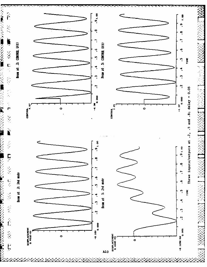
%0
C4C
.in-* ~ "in
I;;: 1
-a.. 4*tooU.n
* a1
'OU
m *m
Nw N
A10
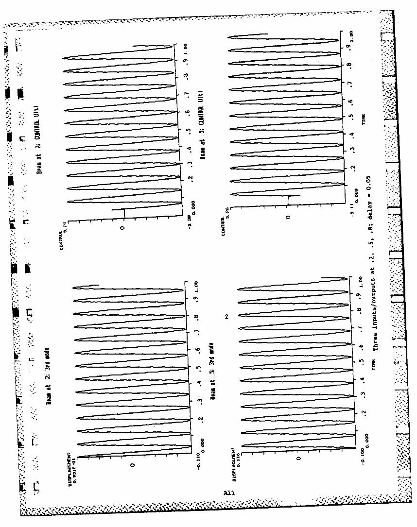
* -
0'4
p.C4 tn
414,
dbpCL
4 U1
p. 4
N IA
S All
.42,
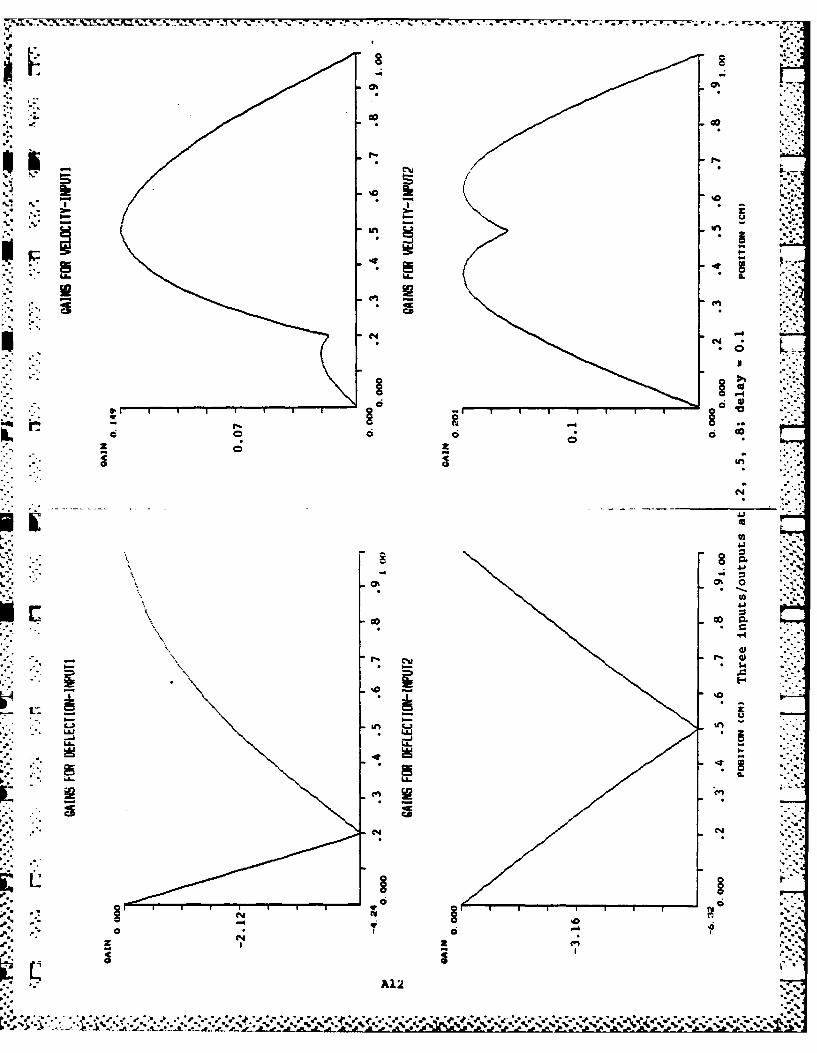
I IL
44
cv
N -.
NIO :N
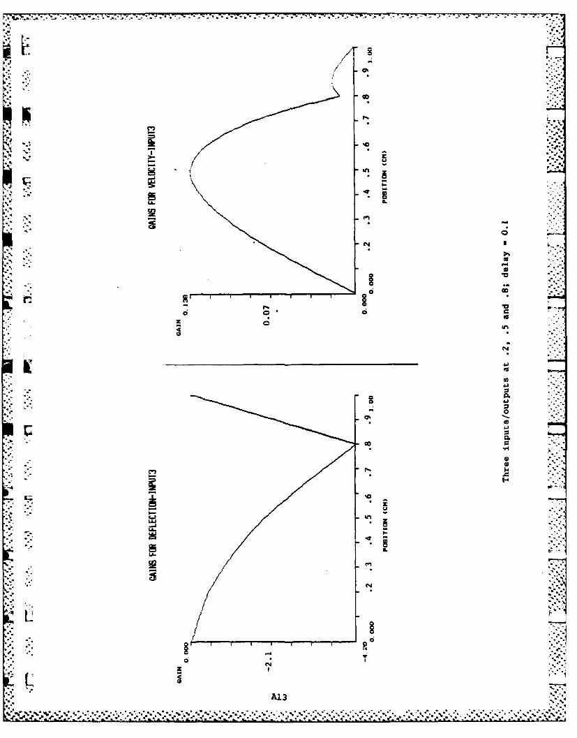
CDC
-~4-j
9-7 I..
CL
CD,
Nk.

." $*,. .
. . .o ,
.U-::,':
4., . : -
( :'.e :
U* U , .
" ,,,Ce, E
* '*C.
* "• U,
• 00 ,
I.- - _ : p.
.. 4: . 4. _/ '_-
4. 4 -:
o 0Le "
A14-"'' "" 'K , I '. " .1""K ' :.A.,", ." ' ". ",. .' ,, ," .'''."% \ "'.".. * , .'.... ',.s ..".. n, " ,'.' ":'. . .."""""""''. ". "., - ~..
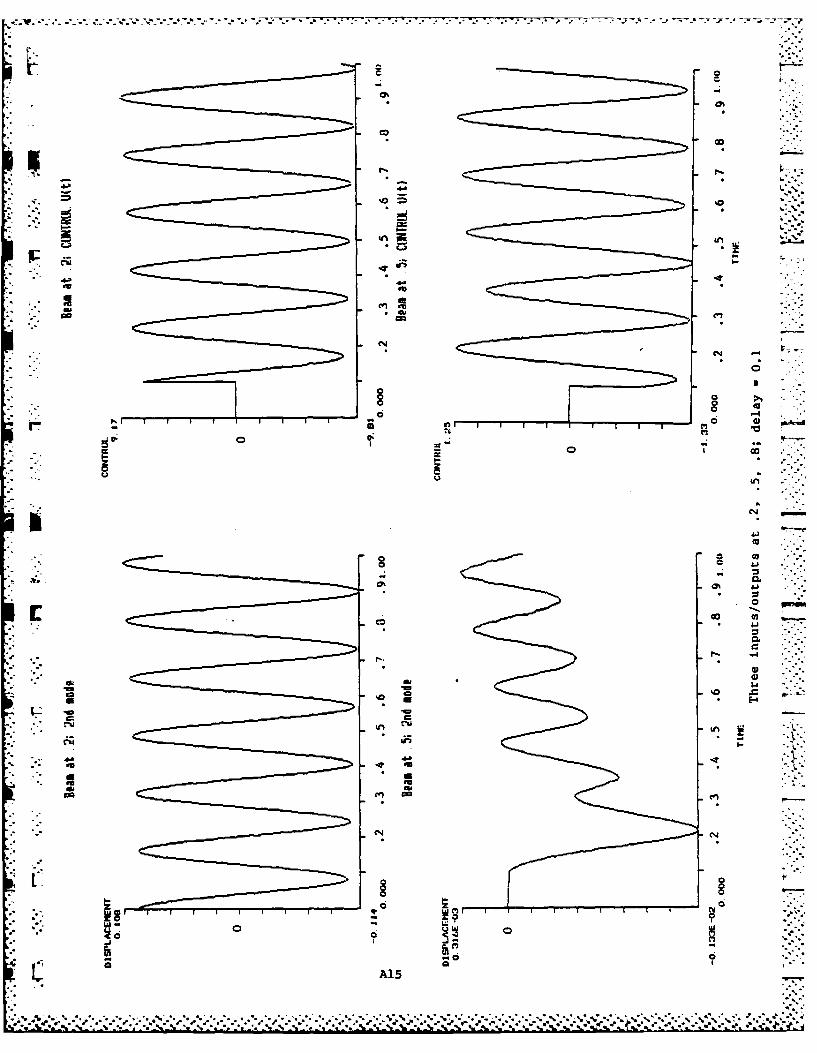
co
00
cS In-
.0 03
ICL
aU
04
I f I I I 0
U. Z, .
AIS_
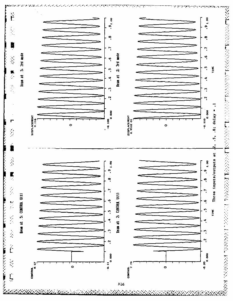
a -E
re r- e
0'
C=,
04
A16

Mcu
* IL
'0
LLI
4 4 04
CM
CI
A17~
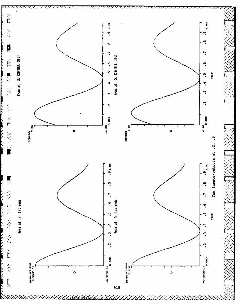
Vi 7 IL
0% 0%
/
9% 9%
.4-
-. mn~ ** V.. ~.. I
I. 9-~. ~-u
4- 4 4.. 4'U * 'U
* - C', a.
NN
§ §r a a
0 .6 0 4
* * - a9-
N
*0
U)4-9
/ S* 4-9
0% 0% 0
U)4-II-'4
09% 9% ~
* s-I
a. a.'0 F
C '0U
* U* 4.8 4.8
* U~ U'
* Ii,9-
4- 4.8'U 4E~ 4U * U'Ua. a.
N N
4 *, I- 0 __________________ 0
* I0
-o 0 0L AJB
* ** 4E.~.. q~I~ .~* ** ~. .~* ** V ~* *.* *.* - * V *. -~ *.~*'.-\*-. -\g...\..--~..- ~* ~ ~~*}i*J*~,J~** ~ ~*****~*4****~***** *..*-**.**.~. - -
~ - - - -*~ ~ 8,~. ~ ~ .* ~. * ~
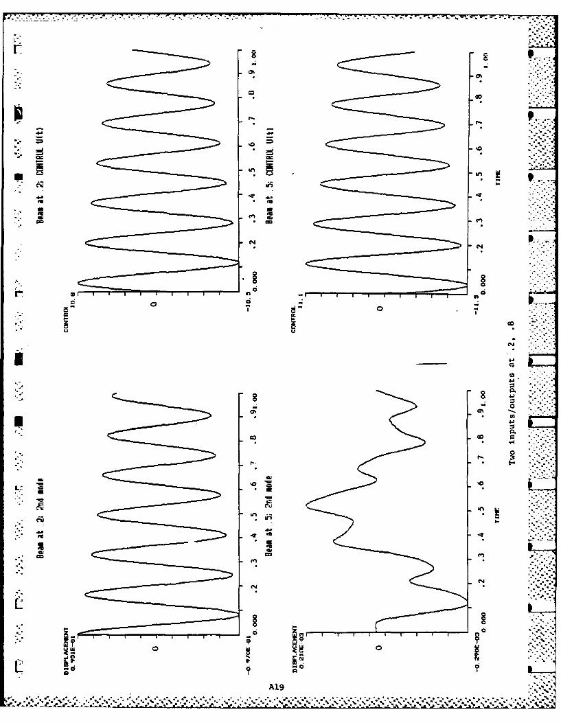
0%0
t0%
'04
to[AIA.
CJ IAGo
4 4., 4
em * Go
* Un
to '
SJ U'
N pA19
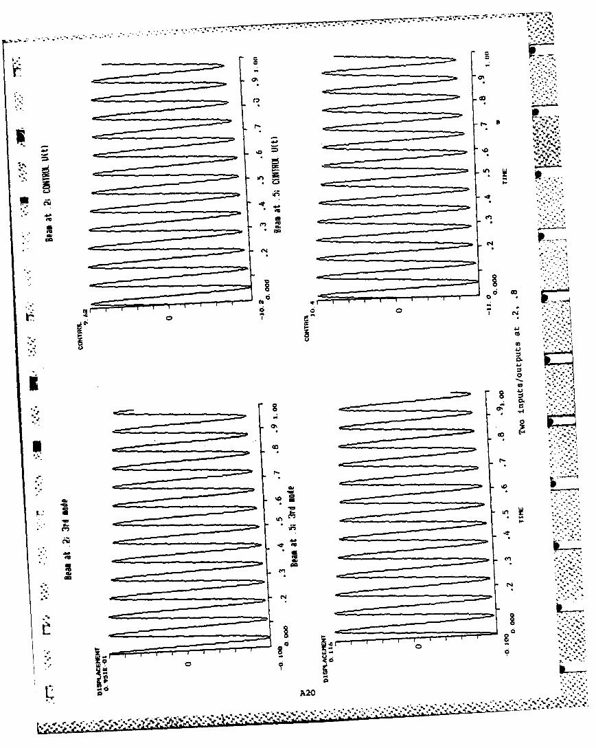
-
* W
a
inC *
am'
N c
'-C A20
i.'.f.f% . *. *C.Vc.*

a ~*. -. . - - - . - -.
8 8
0' -
0'
N
'-a
'a-
* '0* '0
/ Z--8
~j~J'a, En --J S,~ La.J I-
LI.. a. - -
* V CD* b N
N
§ U
'a- 0 0 '-4r 0 a Eno - "Iz * I- 0 z'C
- -4o 'CC a
N
4.1(U
0,4.1*
8N 4-aa'
-* .
a' -a--*
*
1-aa)
a)
0- I--I-
14
*~ '0- I- Uk -
In*~
. -7.LL a.
GD CD
N
N
* * § ___________ ILt a ___________a* Sn q-- ru - 'a- *,X h'
o 0* z -0'C
o "Va..,,
LA2 1
~,'.*a **-,~
a.. ~
J. * ~ ~I t~P~***~ a * * * *- * - *. . % ~ * ~. * *~% %*%**
*~*,*~***.** **a* .,. . .- '.~,'.- .%."..~'.V*'.. * * *
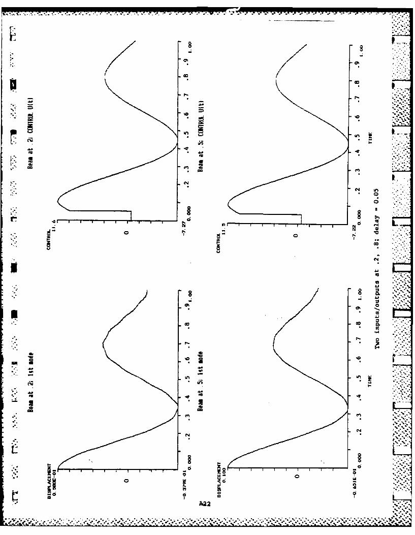
-5 -. 1 T-* I T. T. 9 -9 -. -.-
0% 0 0
I-
4- 4 22
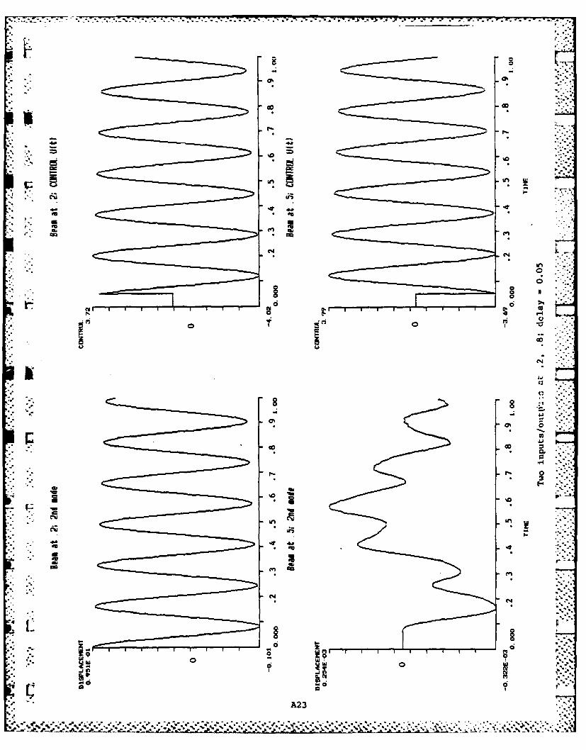
6-. VI-
0-0
0 4.1
in
c-Il
Ig~;01
NoN
Inn
ci0
A20

*I SI
du up *
am.* .3 *~ .0
go* en* u
-g
No
A24A
0 0P.

Pc~0
Oll, '6'. -
A25
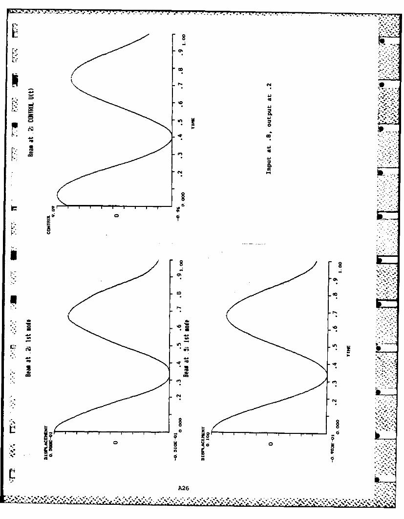
S. k
S.
0%
N
'aU
an 'a
I- 0*3
S
.b.
'aUS 'a
N -
o=
~ -
I-
k
B S
0%
r-.
a. Si
'0S.
Sb.-S
-
-a.. l.a
.~
an _
S. C*~J
an
I-
Eu
4
U
SDEu
.3
.5 ma
S
-cw*~
N
(N
__________ ________
a- C
0 U.
0
II -I~0~0
0a
Cr2* *~ 55555 ~ ~ -X -.
-S * * * * -. ~ ..s:%~: :~;~;~v*.~*. 5 .%;*:%* * ~ <-'
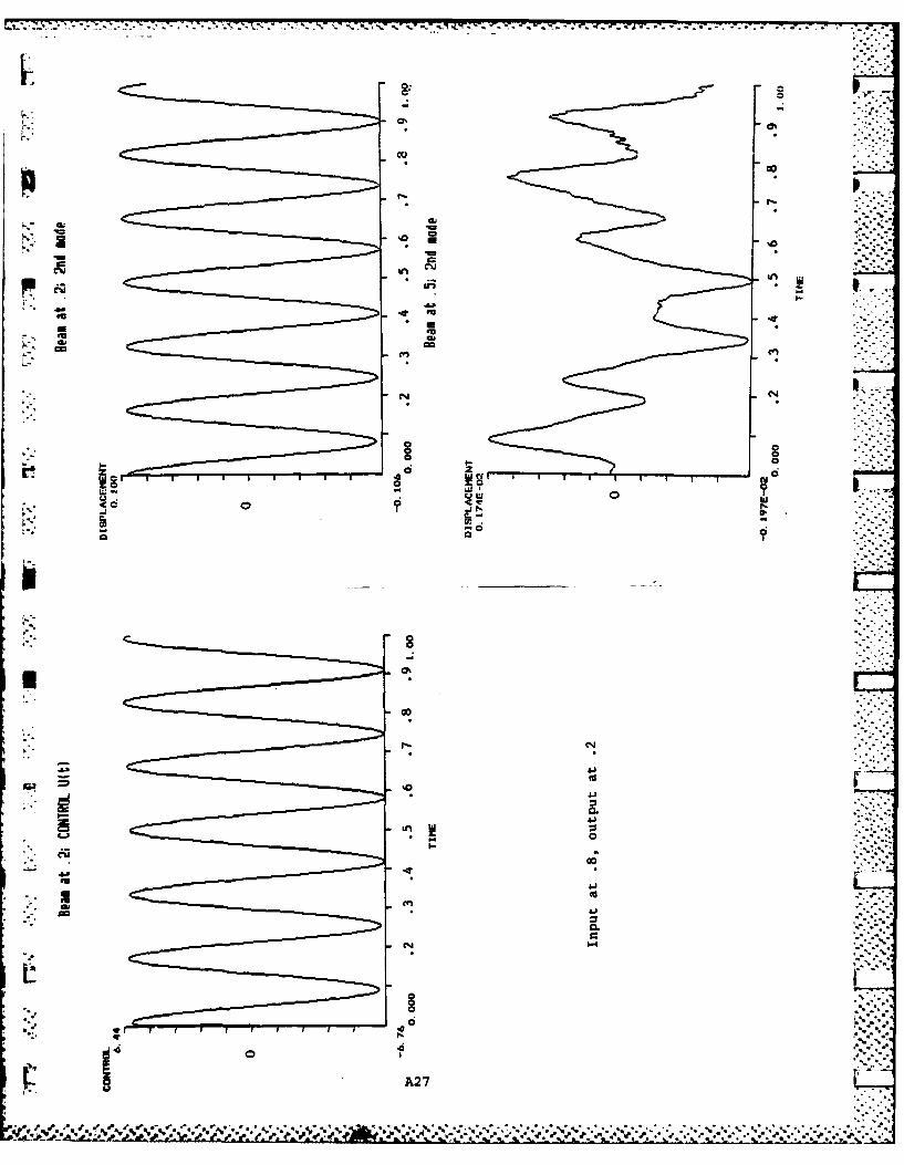
000
ci d
sJi
I.
4W f2U 4U*
r. 'UA27
J, e f e
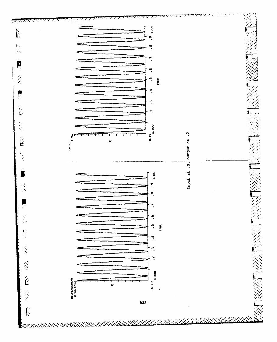
4111
Go'
d-
A2

FILMEL
DTI
Top Related