


Languages
Pages
Legal


Geostatistical Modeling and Upscaling Permeability for Reservoir Scale Modeling in Bioturbated, Heterogeneous Tight Reservoir
Rock: Viking Fm, Provost Field, Alberta
by Amy I. Hsieh
B.Sc. (Earth Sciences), Simon Fraser University, 2013
Thesis Submitted in Partial Fulfillment of the
Requirements for the Degree of
Master of Science
in the
Department of Earth Sciences
Faculty of Science
Amy I. Hsieh 2015
SIMON FRASER UNIVERSITY Summer 2015

ii
APPROVAL
Name: Amy Hsieh
Degree: Master of Science
Title of Thesis: Geostatistical modeling and upscaling permeability for reservoir
scale modeling in bioturbated, heterogeneous tight reservoir
rock: Viking Fm, Provost Field, Alberta
Examining Committee:
Chair: Dr. Andy Calvert
Professor
_______________________________________________
Dr. James MacEachern
Senior Supervisor
Professor
_______________________________________________
Dr. Diana Allen
Co-Supervisor
Professor
_______________________________________________
Dr. Shahin Dashtgard Supervisor
Associate Professor
By video conference from Edmonton Dr. Murray Gingras
External Examiner
Professor, University of Alberta
Date Defended/Approved: August 13, 2015 _
iii
Abstract
While burrow-affected permeability must be considered for characterizing reservoir flow,
the marked variability generated at the bed/bedset scale makes bioturbated media
difficult to model. Study of 28 cored wells of the Lower Cretaceous Viking Formation in
the Provost Field, Alberta, Canada integrated sedimentologic and ichnologic features to
define recurring hydrofacies possessing distinct permeability grades. Transition
probability analysis was employed to model spatial variations in biogenically enhanced
permeability at the bed/bedset scale. Results suggest that variations in permeability are
strongly related to variations in hydrofacies rather than grain size. The variability in
permeability at the bed/bedset scale was simplified by calculating an equivalent
permeability that represents the thickness-weighted sum of permeability at the
bed/bedset scale using expressions for layered media. Numerical block models were
then generated for both the bed/bedset hydrofacies and the upscaled hydrofacies.
Vertical and horizontal flows were simulated at both scales, and the volumetric flows in
each direction were compared to verify the representativeness of the equivalent
permeability. Vertical and horizontal flows simulated for bed/bedset scale and
composite hydrofacies differ by less than 5%, suggesting that permeabilities at the
bed/bedset scale can be simplified through upscaling. Reservoir-scale groundwater flow
was simulated along a hydrogeological cross section comprised of the composite
hydrofacies. The resulting flow regime was consistent with those simulated using
permeability estimates from tight reservoir units of the Viking Formation. This approach
may lead to improved reserve calculations, estimates of resource deliverability, and
understanding of reservoir responses during recovery.
Keywords: Bioturbation; Permeability; Statistical modelling; Upscaling; Numerical Modeling

iv
Dedication
To my Family

v
Acknowledgements
I was lucky to have not one, but two amazing supervisors, Dr. James
MacEachern and Dr. Diana Allen, who continuously guided me throughout the last two
years. Thank you both for your patience, expertise, critiques, and most of all for
strengthening my love of science. I would also like to thank Dr. Shahin Dashtgard and
Dr. Murray Gingras for their insights and suggestions for my thesis, and Kevin Gillen for
his motivation and assistance in the analyses of data.
A very big thank-you goes to my amazing GRRG and ARISE lab mates for all the
fun over the past two years, and especially for your incredible support during the
stressful times that made my hair fall out. I am truly grateful for having you as lifetime
friends. Also, Glenda Pauls, Tarja Vaisanen, Rodney Arnold, and Matt Plotnikoff are
thanked for their endless dedication to the Earth Sciences Department.
Finally, I would like to thank my family for their unconditional support and trust.
Thank you for encouraging me to go off the beaten path…

vi
Table of Contents
Approval .......................................................................................................................... ii Abstract .......................................................................................................................... iii Dedication ...................................................................................................................... iv Acknowledgements ......................................................................................................... v Table of Contents ........................................................................................................... vi List of Tables ................................................................................................................. viii List of Figures................................................................................................................. ix List of Acronyms ............................................................................................................xiv
Introduction ............................................................................................. 1 Chapter 1.1.1. Research Goals and Objectives ............................................................................. 4 1.2. Scope of Work ........................................................................................................ 5 1.3. Overview of Methodology ....................................................................................... 5 1.4. Study Area .............................................................................................................. 8 1.5. Geologic Setting ................................................................................................... 10 1.6. Background .......................................................................................................... 12
1.6.1. Biogenic Modification of Porosity and Permeability .................................. 12 1.6.2. Vertical Transition Probability/Markov Chain Analysis.............................. 16 1.6.3. Reservoir-Scale Modeling ........................................................................ 19
Defining Hydrofacies at Different Scales ............................................. 21 Chapter 2.2.1. Core Logging ........................................................................................................ 21 2.2. Permeability Data ................................................................................................. 22 2.3. Bed to Bedset Scale HFs ...................................................................................... 23 2.4. CHFs Descriptions and Process Interpretations.................................................... 30
2.4.1. CHF 1: Apparently structureless mudstone with siltstone to sandstone interbeds/interlaminae ............................................................ 30
2.4.2. CHF 2: Bioturbated silty to sandy mudstone ............................................ 32 2.4.3. CHF 3: Bioturbated muddy to silty sandstone .......................................... 35 2.4.4. CHF 4: Interbedded mudstone and silty sandstone ................................. 38 2.4.5. CHF 5: Sandstone with mudstone interlaminae/interbeds ........................ 41
2.5. Stratigraphic Cross Sections................................................................................. 42
Statistical Modeling of Biogenically Enhanced Permeability in Chapter 3.Tight Reservoir Rock ............................................................................. 46
3.1. Introduction ........................................................................................................... 46 3.2. Geologic Setting ................................................................................................... 49 3.3. Geostatistics ......................................................................................................... 51 3.4. Methodology ......................................................................................................... 53
3.4.1. Core Logging ........................................................................................... 53 3.4.2. Permeability Data .................................................................................... 54 3.4.3. Hydrofacies and Parameter Class Divisions ............................................ 54 3.4.4. Transition Probability Analysis ................................................................. 56

vii
3.5. Results and Discussion ........................................................................................ 57 3.5.1. Hydrofacies ............................................................................................. 57 3.5.2. Transition Probability (Markov Chain) Analyses ....................................... 62
3.6. Conclusions .......................................................................................................... 65
Upscaling Permeability for Regional Flow Modeling .......................... 67 Chapter 4.4.1. Average Hydraulic Conductivity for Bed to Bedset Scale HFs ............................... 67 4.2. Hydraulic Conductivity Estimation for Composite HFs .......................................... 68 4.3. Validation of Equivalent K ..................................................................................... 69 4.4. Regional Flow Simulations ................................................................................... 75
4.4.1. CHF Model Setup .................................................................................... 75 4.4.2. Additional Simulations Based on Literature K Values .............................. 82 4.4.3. CHF Simulation Results ........................................................................... 84 4.4.4. Results of Flow Simulations using Literature K Values ............................ 88
4.5. Discussion ............................................................................................................ 90
Conclusions ........................................................................................... 92 Chapter 5.5.1. Hydrofacies .......................................................................................................... 93 5.2. Transition Probability Analysis .............................................................................. 93 5.3. Validation of Equivalent K ..................................................................................... 94 5.4. Regional Flow Simulations ................................................................................... 95 5.5. Limitations ............................................................................................................ 95 5.6. Final Remarks ...................................................................................................... 97
References... ................................................................................................................ 98 Appendix A. AccuMap Data ............................................................................... 108 Appendix B. Core Log Data and Geophysical Well Logs .................................... 144 Appendix C. Horizontal Equivalent K .................................................................. 145 Appendix D. Vertical Equivalent K ...................................................................... 148

viii
List of Tables
Table 2.1. Bed/bedset scale hydrofacies descriptions. The calculated kave (mD) or representative kave based on previous studies for each HF are also reported. ................................................................................... 26
Table 3.1. Bed/bedset scale hydrofacies descriptions. The calculated kave (mD) or representative kave based on previous studies for each HF are also reported. ................................................................................... 58
Table 4.1. Bed/bedset scale hydrofacies identified in core and the calculated average hydraulic conductivity (Kave) in m/s or representative Kave based on previous studies for HF 1. Kave values calculated in Chapter 3 are also shown below. ........................................................... 67
Table 4.2. Minimum, maximum, and average horizontal (Kh) and vertical (Kv) conductivities for each composite hydrofacies. ....................................... 75
Table 4.3. Hydraulic conductivity (K) values of the Viking Formation measured in published literature, including the measurement techniques used as well as the lithology in which the measurements were taken. .................................................................... 83
Table 4.4. Global water balance, average hydraulic flux (q) and average hydraulic conductivity (K) from the MODFLOW simulation over cross-section B-B’. ................................................................................. 88
Table 4.5. Hydraulic flux (q) values calculated from MODFLOW results using hydraulic conductivity (K) values published in literature. ......................... 89

ix
List of Figures
Figure 1.1. Flow chart of the methodologies used in this thesis. ................................. 7
Figure 1.2. Map of the study area showing the locations of the wells and cross sections. ................................................................................................... 9
Figure 1.3. Map showing the major hydrocarbon-producing fields of the Viking Formation in Alberta (MacEachern et al. 1999). ..................................... 10
Figure 1.4. Stratigraphic correlation diagram of the Viking Formation in central Alberta showing the overlying Westgate Formation, underlying Joli Fou Formation, as well as its stratigraphic equivalents, the Paddy Member and Bow Island Formation (MacEachern et al., 1999). ............. 11
Figure 1.5. Sand-filled trace fossils, such as Thalassinoides (Th) and Planolites (Pl) create potential flow paths in an otherwise low-permeability unit. Mud-filled traces are dominated by Phycosiphon (Ph). .................................................................................. 15
Figure 2.1. Schematic diagram of the bioturbation index (BI), modified from Reineck (1963), Taylor and Goldring (1993) and Taylor et al. (2003) by MacEachern and Bann (2008). Bioturbation grades correspond to: BI 0 = 0% bioturbation; BI 1 = 1-5% bioturbation; BI 2 = 6-30% bioturbation; BI 3 = 31-60% bioturbation; BI 4 = 61-90% bioturbation; BI 5 = 91-99% bioturbation; and BI 6 = 100%. ................... 24
Figure 2.2. Core log of PCP Verger 14-30-22-16W4. ............................................... 27
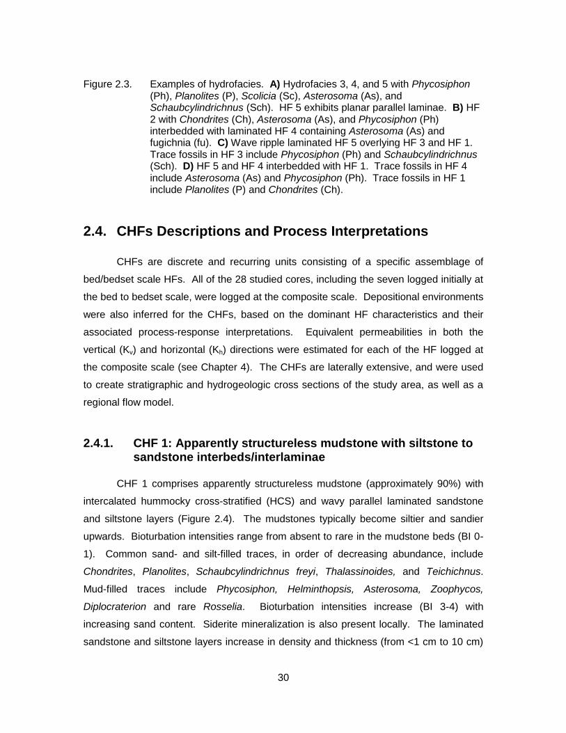
Figure 2.3. Examples of hydrofacies. A) Hydrofacies 3, 4, and 5 with Phycosiphon (Ph), Planolites (P), Scolicia (Sc), Asterosoma (As), and Schaubcylindrichnus (Sch). HF 5 exhibits planar parallel laminae. B) HF 2 with Chondrites (Ch), Asterosoma (As), and Phycosiphon (Ph) interbedded with laminated HF 4 containing Asterosoma (As) and fugichnia (fu). C) Wave ripple laminated HF 5 overlying HF 3 and HF 1. Trace fossils in HF 3 include Phycosiphon (Ph) and Schaubcylindrichnus (Sch). D) HF 5 and HF 4 interbedded with HF 1. Trace fossils in HF 4 include Asterosoma (As) and Phycosiphon (Ph). Trace fossils in HF 1 include Planolites (P) and Chondrites (Ch). ............................................ 30
Figure 2.4. Examples of CHF 1. A) Mudstone showing BI 0-2, with interbedded wavy laminated silty sandstone. Trace fossils include Schaubcylindrichnus freyi (Sf), Phycosiphon (Ph), Asterosoma (As), and Chondrites (Ch). B) Bentonitic mudstone displaying BI 0-1, with laminated silty sandstone lenses. Trace fossils include Chondrites (Ch), Planolites (P), and Asterosoma (As). C) Mudstone showing BI 0-2 with interbedded HCS to planar parallel laminated sandstone and silty sandstone layers. Trace fossils include fugichnia (fu), Chondrites (Ch), Asterosoma (As), and Phycosiphon (Ph). .................................................................................. 32

x
Figure 2.5. Examples of CHF 2. A) Bioturbated silty to sandy mudstone (BI 4) with interbedded structureless mudstone and laminated to structureless sandstone. Trace fossils include Chondrites (Ch), Planolites (P), Asterosoma (As), Diplocraterion (D), Phycosiphon (Ph), Schaubcylindrichnus freyi (Sf), and Zoophycos (Z). B) Bioturbated silty to sandy mudstone (BI 4-5) with interbedded structureless mudstone. Trace fossils include possible Diplocraterion (D?), Chondrites (Ch), Schaubcylindrichnus freyi (Sf), Teichichnus (T), Zoophycos (Z), and Planolites (P). C) Bioturbated silty to sandy mudstone (BI 4-5) with interbedded structureless mudstone. Trace fossils include Planolites (P), Phycosiphon (Ph), possible Diplocraterion (D?), possible Thalassinoides (Th?), Helminthopsis (H), and Asterosoma (A). D) Bioturbated silty to sandy mudstone (BI 4-5) with interbedded structureless mudstone and laminated to structureless sandstone. Trace fossils include Schaubcylindrichnus freyi (Sf), Planolites (P), Chondrites (Ch), Rosselia (Ro), Phycosiphon (Ph), and Asterosoma (As). E) Bioturbated silty to sandy mudstone (BI 5). Trace fossils include Thalassinoides (Th), Zoophycos (Z), Asterosoma (As), Planolites (P), Phycosiphon (Ph), Schaubcylindrichnus freyi (Sf), and Chondrites (Ch). ............................. 35
Figure 2.6. Examples of CHF 3. A) Lower very fine- to lower fine-grained bioturbated muddy to silty sandstone. Units show BI 4-5. Trace fossils include Asterosoma (As), Planolites (P), Zoophycos (Z), Phycosiphon (Ph), Schaubcylindrichnus freyi (Sf), and Diplocraterion (D). B) Lower fine-grained bioturbated silty sandstone (BI 4-5) with interbedded mudstone and laminated sandstone. Trace fossils include Palaeophycus (Pa), Asterosoma (As), Planolites (P), Siphonichnus (Si), Chondrites (Ch) and fugichnia (fu). C) Lower fine-grained bioturbated muddy to silty sandstone (BI 4-5) with interbedded mudstone and laminated sandstone. Trace fossils include Schaubcylindrichnus freyi (Sf), Chondrites (Ch), Teichichnus (T), Asterosoma (As), Planolites (P), Diplocraterion (D), Palaeophycus (Pa), and Thalassinoides (Th). D) Lower fine-grained bioturbated muddy to silty sandstone (BI 5). Trace fossils include Diplocraterion (D), Phycosiphon (Ph), Planolites (P), Rhizocorallium (Rh), Chondrites (Ch), and Asterosoma (As). E) Lower very fine-grained bioturbated muddy to silty sandstone (BI 4-5). Trace fossils include Schaubcylindrichnus freyi (Sf), Chondrites (Ch), Phycosiphon (Ph), Planolites (P), Teichichnus (T), and Asterosoma (As). F) Lower fine-grained bioturbated silty sandstone (BI 4-5) with interbedded mudstone and laminated sandstone. Trace fossils include Phycosiphon (Ph), Schaubcylindrichnus freyi (Sf), Chondrites (Ch), Planolites (P), and Rosselia (Ro). ................................ 38

xi
Figure 2.7. Examples of CHF 4. A) Interbedded mudstone and silty sandstone. The mudstone beds are structureless, and the sandstone beds exhibit planar parallel laminae. Units show BI 0-2. The trace -fossil suite includes Thalassinoides (Th), Chondrites (Ch), Diplocraterion (D), Planolites (P), and Phycosiphon (Ph). B) Apparently structureless mudstone, interbedded with planar parallel to wavy laminated silty sandstone. Bioturbation intensities range from BI 0-3. Trace fossils include fugichnia (fu), Planolites (P), Phycosiphon (Ph), Chondrites (Ch), and possible Skolithos (Sk?). C) Interlaminated mudstone and silty sandstone with bentonite cementation. Units show BI 0-1. Trace fossils are diminutive and include Planolites (P), Chondrites (Ch), and Phycosiphon (Ph). D) Apparently structureless mudstone interbedded with laminated silty sandstone. ........................................... 41
Figure 2.8. Examples of CHF 5. A) Lower medium-grained sandstone with low-angle planar parallel laminae and possible cryptic bioturbation. B) Wavy laminated, upper fine-grained sandstone. Unit shows BI 0-1. Trace fossils include Chondrites (Ch) and Zoophycos (Z). C) Lower medium-grained sandstone with HCS. The rip-up clast (rc) layer in the photo is likely composed of eroded and transported fragments of Rosselia, Palaeophycus, or Asterosoma. D) Lower medium-grained sandstone. The trace-fossil suite includes Rosselia (Ro), possible Asterosoma (As?), Chondrites (Ch), Skolithos (Sk), Planolites (P), and Phycosiphon (Ph). ....................................................................................................... 42
Figure 2.9. Stratigraphic cross-section A-A’ constructed using composite hydrofacies (CHF). ................................................................................. 44
Figure 2.10. Stratigraphic cross-section B-B’ constructed using composite hydrofacies (CHF). ................................................................................. 45
Figure 3.1. Sand-filled trace fossils such as Thalassinoides (Th) and Planolites (Pl) create potential flow paths in an otherwise low-permeability unit. Mud-filled traces are dominated by Phycosiphon (Ph). .................................................................................. 48
Figure 3.2. Map showing the major hydrocarbon-producing fields of the Viking Formation in Alberta (MacEachern et al., 1999). .................................... 49
Figure 3.3. Stratigraphic correlation diagram of the Viking Formation in central Alberta showing the overlying Westgate Formation, underlying Joli Fou Formation, as well as its stratigraphic equivalents, the Paddy Member and Bow Island Formation (MacEachern et al., 1999). ............. 50
Figure 3.4. Schematic diagram of the bioturbation index (BI), modified from Reineck (1963), Taylor and Goldring (1993) and Taylor et al. (2003) by MacEachern and Bann (2008). Bioturbation grades correspond to: BI 0 = 0% bioturbation; BI 1 = 1-4% bioturbation; BI 2 = 5-30% bioturbation; BI 3 = 31-60% bioturbation; BI 4 = 61-90% bioturbation; BI 5 = 91-99% bioturbation; and BI 6 = 100%. ................... 55

xii
Figure 3.5. Example of a Markov chain transiogram. The transition probability value at which the curve reaches its limit is the “sill”. The lag distance at which the Markov chain reaches the sill is the “range”. The slope of the tangent line is the transition rate of the material, and the point at which the tangent line intersects the x-axis is the mean les length of the material. ............................................................. 56
Figure 3.6. Core log of PCP Verger 14-30-22-16W4. ............................................... 59
Figure 3.7. Examples of hydrofacies. A) Hydrofacies (HF) 3, 4, and 5 with Phycosiphon (Ph), Planolites (P), Scolicia (Sc), Asterosoma (As), and Schaubcylindrichnus (Sch). HF 5 exhibits planar parallel laminae. B) HF 2 with Chondrites (Ch), Asterosoma (As), and Phycosiphon (Ph) interbedded with laminated HF 4 containing Asterosoma (As) and fugichnia (fu). C) Wave ripple laminated HF 5 overlying HF 3 and HF 1. Trace fossils in HF 3 include Phycosiphon (Ph) and Schaubcylindrichnus (Sch). D) HF 5 and HF 4 interbedded with HF 1. Trace fossils in HF 4 include Asterosoma (As) and Phycosiphon (Ph). Trace fossils in HF 1 include Planolites (P) and Chondrites (Ch). ............................................ 62
Figure 3.8. Vertical transition probability matrix for kmax (solid black line) vs. grain size (dashed gray line). fL: lower fine-grained; fU: upper fine-grained; mL: lower medium-grained. ............................................... 63
Figure 3.9. Vertical transition probability matrix for kmax (solid black line) vs. hydrofacies (dotted gray line). ................................................................ 64
Figure 4.1. Upscaling hydraulic conductivity (K) at the bed to bedset scale to a single equivalent hydraulic conductivity in both the vertical (Kv) and horizontal (Kh) directions for a composite hydrofacies using the expressions for layered media (see Equations 4.1 and 4.2). ............ 68
Figure 4.2. Boundary conditions for A) horizontal flow simulations and B) vertical flow simulations. h refers to the assigned hydraulic head. ......... 70
Figure 4.3. A) Example of a MODFLOW block model of a cored section with hydrofacies logged at the bed/bedset scale. Each colour represents a different hydrofacies. B) Block model of the same cored section with hydrofacies logged at the composite scale. ............... 72
Figure 4.4. Discharge in Q (m3/s) for bed/bedset scale and composite scale fluid flow simulations in the A) horizontal and B) vertical directions. ....... 74
Figure 4.5. Hydrogeological cross-section B-B’ constructed using Composite Hydrofacies (CHF). ................................................................................ 76
Figure 4.6. Contours of hydraulic head in the Viking Formation, showing the locations of cross-sections A-A’ and B-B’. Contour intervals are in metres. The solid black arrow shows the simplified direction of the groundwater flow, and the dotted gray arrows show actual groundwater flow directions (Modified after Bachu et al., 2002). Estimates of the hydraulic head are shown for the ends of each cross section. ......................................................................................... 78

xiii
Figure 4.7. MODFLOW domain for hydrogeological cross-section B-B’ showing the hydraulic heads (h) at the NW and SE boundaries. ............ 81
Figure 4.8. Equipotential head contour map of cross-section B-B’. Contour units are in metres. The zoomed section illustrates the deviation of flow lines in red arrows. The maximum arrow length
corresponds to a maximum velocity of 4.610-4 m/s, to which all other vectors are scaled. ........................................................................ 85
Figure 4.9. Fluid flow velocity vector map for cross-section B-B’. The maximum arrow length corresponds to a maximum velocity of
4.610-4 m/s, to which all other vectors are scaled. ................................ 87
Figure 4.10. Distribution of hydraulic flux (q) values calculated using ranges of Viking Formation hydraulic conductivities found in literature. The q from the CHF simulation falls between 10-12 and 10-11 m/s. ................. 90

xiv
List of Acronyms
BI Bioturbation Index (grades of bioturbation intensity)
CHF Composite hydrofacies
fL Lower fine-grained
fU Upper fine-grained
GMS Groundwater Modelling Software
h Hydraulic head
HCS Hummocky cross-stratification
HF Hydrofacies
K Hydraulic conductivity
kave Average permeability
Kave Average hydraulic conductivity
Kh Horizontal hydraulic conductivity
kmax Maximum permeability
Kv Vertical hydraulic conductivity
mL Lower medium-grained
Q Discharge
q Darcy flux
rc Rip-up clast
T-PROGS Transition Probability Geostatistical Software
Trace Fossils
As Asterosoma
Ch Chondrites
D Diplocraterion
fu fugichnia
P Planolites
Pa Palaeophycus
Ph Phycosiphon
Rh Rhizocorallium
Ro Rosselia
Sc Scolicia

xv
Sch Schaubcylindrichnus coronus
Sf Schaubcylindrichnus freyi
Sk Skolithos
T Teichichnus
Th Thalassinoides
Z Zoophycos

1
Chapter 1. Introduction
The storage capacity and productivity of a reservoir are determined by its
porosity and permeability. Permeability is also an important factor that controls reservoir
response during enhanced hydrocarbon recovery. Correspondingly, understanding and
projecting variations in porosity and permeability within a reservoir are vital to
maximizing the acquisition of the resource. Recently, there has been considerable
interest in recovering hydrocarbons from marginal (generally lower-quality) reservoirs
using horizontal drilling techniques and fracturing, particularly in areas prone to light oil.
The so-called “Tight Oil” play of the Viking Formation in east-central Alberta and west-
central Saskatchewan constitutes one example. “Tight” reservoirs are characterized by
permeabilities that range from 0.01–0.1 mD (Spencer, 1989; Holditch, 2006; Clarkson
and Pedersen, 2010). In such reservoirs, subtle changes in the distribution of
sedimentary media, such as that generated by bioturbation, can greatly affect the
porosity and permeability distribution of the facies.
Bioturbation remains an under-appreciated mechanism by which porosity and
permeability of a sedimentary facies are modified (cf. Pemberton and Gingras, 2005).
Even when considered, bioturbation is generally perceived to be detrimental to bulk
permeability, through reduction of primary grain sorting, homogenization of the sediment,
and introduction of mud through linings, biogenic deposits, and feces (Qi, 1998; Dornbos
et al., 2000; Qi et al., 2000; McDowell et al., 2001; Pemberton and Gingras, 2005;
Tonkin et al., 2010; Lemiski et al., 2011; La Croix et al., 2013). Recent studies have
shown, however, that several ichnogenera and their associated biogenic fabrics are
capable of increasing a reservoir rock’s porosity and permeability (Gingras et al., 2004;
Pemberton and Gingras, 2005; Hovikoski et al., 2007; Volkenborn et al., 2007;
Cunningham et al., 2009; Tonkin et al., 2010; Lemiski et al., 2011; Gingras et al., 2012;

2
La Croix et al., 2013; Knaust, 2014). Ichnogenera that form branching burrow networks
can create flow pathways in otherwise less permeable units where the burrow fills
consist of coarser grains and better-connected intergranular pore space relative to the
surrounding matrix (Gingras et al., 2004; Pemberton and Gingras, 2005; Lemiski et al.,
2011; Gingras et al., 2012; La Croix et al., 2013). Additionally, burrows are capable of
increasing vertical permeability in laminated sedimentary rocks where horizontal
permeability tends to dominate (Gingras et al., 2012). Burrow fills also may undergo
diagenetic changes that may lead to higher permeability than that of the surrounding
matrix (Pemberton and Gingras, 2005; Tonkin et al., 2010; Gingras et al., 2012).
Despite increasing evidence of biogenic enhancement of permeability and
porosity, permeability across unfractured sedimentary reservoirs is commonly assessed
solely on the basis of average grain size (e.g., lithostratigraphic units). Indeed,
bioturbation is generally neglected in permeability assessments of rock units owing to
the complexity of bioturbated media (Gingras et al., 2012). Unless bioturbation
intensities are high, and the burrows are filled with (i) a contrasting lithology, (ii) coarser
sediment, or (iii) media with different degrees of sorting relative to the surrounding matrix
(e.g., abundant mud-filled traces in a sandstone matrix), burrowed and unburrowed units
are assigned the same permeability values. This is particularly problematic in tight
oil/gas reservoirs, where even small disturbances in the sedimentary fabric caused by
bioturbation can significantly increase permeability in these otherwise impermeable units
(e.g., Pemberton and Gingras, 2005; Hovikoski et al., 2007; Gingras et al., 2012; La
Croix et al., 2013; Knaust, 2014).
While burrow-affected permeability trends in reservoirs must be considered in
order to properly characterize reservoir parameters, the marked variability generated at
the bed to bedset scale makes such bioturbated media difficult to model. To simulate
flow in such heterogeneous media, the spatial variations in hydraulic conductivity must
be characterized accurately to simulate the true geologic and hydrogeologic
heterogeneities that are observed and measured in core (Park et al., 2004). Instead of
defining permeability on the basis of average grain size alone, herein the use of
“hydrofacies” (HF) in reservoir characterization is proposed. Such a “hydrofacies” is

3
defined as a recurring unit possessing a distinct permeability that is associated with a
combination of sedimentological and ichnological characteristics.
To analyze vertical and lateral facies relationships, and to characterize
subsurface heterogeneities and uncertainties, geostatistical methods based on Walther’s
Law can be applied. Walther’s Law states:
The various deposits of the same facies area and similarly the sum of the rocks of different facies areas are formed beside each other in space, though in cross section we see them lying on top of each other. As with biotopes, it is a basic statement of far-reaching significance that only those facies and facies areas can be superimposed primarily which can be observed beside each other at the present time.
(Walther, 1894 as translated by Middleton, 1973).
This law implies that sedimentary environments tend to experience gradual spatial shifts
with time (cf. Dalrymple, 2010). Thus, the occurrence of biogenically induced permeable
layers may be statistically predictable by understanding the cyclic repeatability of
sedimentary processes.
Traditionally, geostatistical models such as variograms, coupled with data
interpolation, have been used to simulate spatial variability in the hydraulic properties of
geologic media. These methods, however, have strict requirements (e.g., Gaussian
distribution, stationarity) that are unrealistic in geologic environments. In addition, these
methods may generate results that are too smooth and continuous, particularly in data-
sparse areas (Park et al., 2004). Alternatively, a more intuitive, mathematically compact,
and theoretically effective method was proposed by Carle and Fogg (1996) – a transition
probability approach coupled with Markov chain analysis – which permits the integration
and subjective interpretation of geologic data (Park et al., 2004).
In this thesis, transition probability analysis is explored as a possible statistical
tool for modeling the spatial variations in biogenically enhanced permeability at the small
scale (bed and bedset scales as expressed in core), and for defining “hydrofacies”. An
approach is tested for logging “hydrofacies” at a composite scale and assigned
“upscaled” permeability values that can be used for reservoir-scale modeling. Such an

4
approach may lead to improved reserve calculations, estimates of resource
deliverability, and understanding of reservoir response throughout all stages of recovery.
1.1. Research Goals and Objectives
To characterize heterogeneous, “tight” reservoirs, it is necessary to consider not
only the lithologic, but the biogenic and hydraulic properties of the facies as well.
Different “hydrofacies” could be defined based on properties. The combination of these
properties at the bed to bedset scale, which can be observed in core, then need to be
upscaled in order to model permeability trends at the three-dimensional reservoir scale.
This requires not only a means to map “hydrofacies” at the reservoir scale, but also a
method to assign appropriate upscaled hydraulic properties to those composite
“hydrofacies”.
The purpose of this study is to explore the use of Markov transition probability
analysis in combination with conventional core logging techniques and permeability data
as a means for defining “hydrofacies” and their associated hydraulic properties at two
scales: the bed to bedset scale and the composite scale. The study is focused on a
biogenetically enhanced reservoir from the Viking Formation of the Provost Field,
Alberta. The study integrates sedimentology, ichnology, hydrogeology, and geostatistics
to characterize flow in bioturbated, heterogeneous media.
The objectives of the research are:
1. To establish criteria that define hydrofacies (HF).
2. To explore the transition relations between permeability and various properties measureable at the bed/bedset and composite scales, including sedimentology and ichnology, as a means to identify which parameter (or combination of parameters) best reflects the permeability transitions.
3. To estimate and verify the equivalent permeability for each composite hydrofacies.
4. To test the use of upscaled composite hydrofacies for representing geological heterogeneity in a flow model.

5
1.2. Scope of Work
The following tasks were undertaken for this research:
Objective 1:
1. Core logging at the bed/bedset scale and composite scale of selected cores within the Viking Formation of the Provost Field, Alberta.
2. Defining different hydrofacies based on lithology, sedimentary structures, sedimentary accessories, ichnological suites, bioturbation index (BI), grain size, porosity, and permeability.
Objective 2:
1. Using the T-PROGS software (GMS version 6.0, Copyright © 2013 Aquaveo) to produce vertical transition probability matrices for permeability, average grain size, and bed/bedset hydrofacies to identify which parameter (or combination of parameters) best reflects the permeability transitions.
Objective 3:
2. Estimating equivalent permeability for composite hydrofacies using the multi-layer equivalent permeability approach.
3. Generating block models using the defined bed/bedset scale and composite scale hydrofacies and their corresponding equivalent permeability values to evaluate whether the upscaled hydrofacies yield consistent results with the bed/bedset hydrofacies representations.
Objective 4:
4. Constructing a cross section in the direction of the regional hydraulic gradient and the regional structural dip of the study area using the composite hydrofacies and their corresponding equivalent permeability values, and then simulating flow along the cross section using MODFLOW.
1.3. Overview of Methodology
The methodology used in this research project involved a combination of steps
as shown in Figure 1.1:

6
1. Core logging the bed to bedset scale and identification of bed to bedset scale hydrofacies (HFs).
2. Permeability analyses from plug and full-diameter core measurements (kmax).
3. Transition probability analysis for evaluating the bed to bedset scale HFs as an indicator of permeability.
4. Calculation of average hydraulic conductivities (Kave) for each HF identified at the bed to bedset scale.
5. Core logging according to composite HFs. 6. Estimation of the “upscaled” equivalent hydraulic conductivity in both the
horizontal (Kh) and vertical (Kv) directions for the composite HFs using the Kave values for the bed to bedset scale HFs.
7. Validation of the equivalent hydraulic conductivities using numerical flow modeling.
8. Regional numerical flow modeling along a cross section in the study area using the “upscaled” equivalent hydraulic conductivities for the composite HFs.

7
Figure 1.1. Flow chart of the methodologies used in this thesis.

8
1.4. Study Area
The study area (Figure 1.2) for this research project lies within the Provost Field
of southeastern Alberta, Canada. Twenty-nine cored sections of the Viking Formation
were selected for this project. Wells of the Viking Formation were chosen because the
hydrocarbon-producing successions in the area consist of tight sandstones that exhibit
interlayering of impermeable and permeable beds with variable but locally pervasive
bioturbation. The type, distribution, and intensity of bioturbation are influenced by both
allogenic and autogenic variations in the sedimentary environment (e.g., MacEachern et
al., 2010). The trace-fossil suites observed in the facies successions reflect proximal-
distal as well as along-strike shifts in the causative environment. The cores selected
were drilled post-1970s, have core analysis data, and extend for two townships and
three ranges in area (TP 34-35, R08-10W4M; representing and area of approximately
530 km2).

9
Figure 1.2. Map of the study area showing the locations of the wells and cross sections.

10
1.5. Geologic Setting
The Lower Cretaceous (Upper Albian) Viking Formation is a prolific oil- and gas-
producing interval that was deposited in the Western Canada foreland basin during a
period of active tectonism and eustatic sea level fluctuations. During Viking deposition,
a shallow epicontinental seaway extended from the Arctic Ocean to the Gulf of Mexico
(Figure 1.3; Williams and Stelck, 1975; Caldwell, 1984; Walker, 1990; Reinson et al.,
1994), into which was deposited a complex succession of mudstones, heterolithic
bedsets of sandstone and shale, sandstones, and minor conglomerates.
Figure 1.3. Map showing the major hydrocarbon-producing fields of the Viking Formation in Alberta (MacEachern et al. 1999).
The Viking Formation stratigraphically overlies the Joli Fou Formation and
underlies the Westgate Formation (Figure 1.4; Stelck, 1958). It is generally regarded to
be roughly equivalent to the Paddy Member of the Peace River Formation of

11
northwestern Alberta (Leckie et al., 1990), and the Bow Island Formation of southern
Alberta and southwestern Saskatchewan (Figure 1.4; Stelck and Koke, 1987;
Raychaudhuri and Pemberton, 1992). The stratigraphic relationships were addressed
by the work of Stelck (1958), Glaister (1959), McGookey et al. (1972), Weimer (1984),
Cobban and Kennedy (1989), Stelck and Leckie (1990), Bloch et al. (1993), Caldwell et
al. (1993), and Obradovich (1993).
Figure 1.4. Stratigraphic correlation diagram of the Viking Formation in central Alberta showing the overlying Westgate Formation, underlying Joli Fou Formation, as well as its stratigraphic equivalents, the Paddy Member and Bow Island Formation (MacEachern et al., 1999).
The Upper Albian Viking Formation comprises a siliciclastic succession mainly
reflecting shoreface, delta and estuarine incised valley deposits (cf. Boreen and Walker,
1991; Pattison, 1991; Pattison and Walker, 1994; Reinson et al., 1994; Walker, 1995;
Burton and Walker, 1999; MacEachern et al., 1999; Dafoe et al., 2010). These clastic
sediments were supplied from the rising Cordillera in the west and reflect northward and
eastward progradation of environments into the Alberta foreland basin.

12
Despite the Viking deposits only ranging from 15 to 30 m in thickness, they are
discontinuity bound and depositionally complex, resulting in sedimentary successions,
facies, and geometries that are challenging to characterize and correlate. Beaumont
(1984), Boreen and Walker (1991), Pattison (1991), Posamentier and Chamberlain
(1993), Reinson et al. (1994), Pattison and Walker (1994), Walker (1995), Burton and
Walker (1999), and MacEachern et al. (1999), among others, have attempted to provide
allostratigraphic and sequence stratigraphic assessments of the Viking, with varying
levels of success. Viking Formation discontinuities have been linked to the global
changes of sea level outlined in Kauffman (1977), Vail et al. (1977), Weimer (1984), and
Haq et al. (1987). A cored interval of the Viking Formation from the Verger Field was
selected for this study because it exhibits stacked parasequences characterized by the
interstratification of impermeable and permeable beds with variable but locally pervasive
bioturbation.
1.6. Background
1.6.1. Biogenic Modification of Porosity and Permeability
Bioturbation is the modification of sedimentary media by epifaunal and/or
endobenthic organisms. It includes tracks, trails, burrows, feeding structures, and
escape structures. These features are not the organisms themselves, but instead a
record of the organisms’ activities in the environment. The distribution of trace-fossil
assemblages is largely controlled by complex environmental factors, including sediment
type, substrate consistency, sediment grain size, food-resource types, energy
conditions, salinity, oxygenation, water turbidity, and deposition rate (e.g., Ekdale et al.,
1984; Pemberton et al., 1992; MacEachern et al., 2005; Gingras et al., 2007).
Softground trace-fossil assemblages reflect the condition(s) of the sedimentary
environment in which the trace-making animals lived. Organisms and their
corresponding burrowing behaviours are extremely sensitive to changes in their habitats
and, as a result, trace fossils provide excellent indicators of changing depositional
conditions at various temporal scales.

13
In sedimentary geology, autogenically induced sedimentary cycles are
depositional events that recur within a single sedimentary system and result from
changes that are intrinsic to the system (cf. Beerbower, 1964; Cecil, 2003). The effects
of these autogenic events tend to range from local to regional (e.g., from current ripple
migration through channel migration, to avulsion-driven delta lobe switches or lateral
shifts of submarine fan lobes). These events may be periodic and occur geologically
instantaneously (Reading, 1996). Allogenically induced sedimentary cycles, on the other
hand, comprise recurring events that are imposed externally on the sedimentary system
(cf. Beerbower, 1964; Cecil, 2003). Examples of allogenic events include effects of
climate change, Milankovitch processes and orbital forcing, and tectonically or
eustatically driven sea-level changes, although the latter two are more aperiodic
(Reading, 1996). Progressive recurring changes in depositional conditions owing to
shifts of environments (either autogenically or allogenically induced) can be marked by
cyclic changes in the resulting rock properties (e.g., Bernard and Major, 1963; Krumbein
and Sloss, 1963; Beerbower, 1964; Reading, 1996). This includes changes in
bioturbation intensity and trace-fossil assemblages (e.g., Pemberton et al., 1992; Taylor
et al., 2003; McIlroy, 2004; MacEachern et al., 2010).
It is generally assumed that bioturbation reduces porosity and permeability by
altering grain sorting, disturbing primary sedimentary layering, "piping" sediment and
fluids between sedimentary units, adding or removing organic matter and clay, creating
pathways for mineralizing pore fluids, or changing pore fluid chemistries (e.g., McDowell
et al., 2001; Pemberton and Gingras, 2005; Tonkin et al., 2010). By contrast, some
studies have shown that bioturbation is capable of enhancing bulk permeability and
vertical permeability in otherwise impermeable or marginally permeable rock units (e.g.,
Gingras et al., 1999; Pemberton and Gingras, 2005; Gingras et al., 2007; Tonkin et al.,
2010; Baniak et al., 2012). For example, in their study of the Upper Cretaceous
Medicine Hat Formation of Alberta, Canada, La Croix et al. (2013) demonstrated that
several ichnogenera served to improve permeability by approximately two orders of
magnitude compared to the unburrowed matrix.
In the Upper Triassic Montney Formation of northeastern British Columbia and
the Upper Cretaceous Alderson Member of southwestern Saskatchewan, spot

14
permeability tests show that small and interconnected Phycosiphon are associated with
increased porosity and permeability values (0.23–30.4 mD) compared to those of the
surrounding matrix (0.02–0.06 mD; Hovikoski et al., 2007 and Lemiski et al., 2011,
respectively). These studies show that bioturbation is analogous to natural fractures,
with large surface areas capable of enhancing flow within lower permeability units
(Lemiski et al., 2011).
Volkenborn et al. (2007) provide a modern analogue of biogenically enhanced
permeability by the burrowing of lugworms (Arenicola marina). This large-scale
experiment of lugworms in 400 m2 of intertidal fine-grained sand showed that not only
are these polychaetes capable of significantly increasing porosity and permeability by
creating flow paths through their burrows, but that a lack of these infauna resulted in an
influx of organic particles that obstructed the pores, causing an eight-fold decrease in
permeability. These results show the effectiveness of bioturbation in creating and
maintaining a permeable condition within some sedimentary facies (Volkenborn et al.,
2007).
Examples of biogenically enhanced reservoirs also include the Biscayne aquifer
in Florida (Cunningham et al., 2009) and the Ghawar Field of Saudi Arabia (Pemberton
and Gingras, 2005). The highly permeable layers of the Biscayne aquifer (known as
“Super K” zones) are the result of Thalassinoides- and Ophiomorpha-induced
macroporosity networks, coupled with minor moldic porosity from the dissolution of
fossils (Figure 1.5; Cunningham et al., 2009). The Hawiyah portion of the Ghawar Field
in Saudi Arabia also exhibits such “Super K” zones, generated by firmground
(palimpsest) Thalassinoides boxworks filled with detrital sucrosic dolomite (Pemberton
and Gingras, 2005). These palimpsest burrows have diameters ranging from 1–2 cm
and lengths of up to 2.1 m (La Croix et al., 2013).
Permeable flow paths created by bioturbation result from lithological contrast
between the trace-fossil fill and the rock matrix (Figure 1.5), changes in sorting, and/or
geochemical heterogeneities within the matrix (Tonkin et al., 2010). Biogenic flow paths
occur in both clastic and carbonate reservoirs, wherein burrow fills consist of differing
lithologies, sediment calibres, or degrees of sorting relative to those of the host

15
substrate; and correspondingly may be subject to different diagenetic processes
(Pemberton and Gingras, 2005).
Figure 1.5. Sand-filled trace fossils, such as Thalassinoides (Th) and Planolites (Pl) create potential flow paths in an otherwise low-permeability unit. Mud-filled traces are dominated by Phycosiphon (Ph).
The morphology and density of traces constitute important factors in the resulting
porosity and permeability distributions (La Croix et al., 2013). For example, whereas
both Ophiomorpha and Thalassinoides tunnels are large in diameter and prone to
branching geometries, laboratory analyses show that Ophiomorpha may be less
effective at enhancing permeability and may even reduce permeability owing to their
pelleted mud linings (Tonkin et al., 2010). In addition to the density of bioturbation and
size of burrows, the geometry of the ichnogenera can affect the connectivity of flow
pathways. Burrows that branch both vertically and horizontally such as Thalassinoides
are more effective in creating an isotropic flow network (La Croix et al., 2013). Trace
fossils that do not branch, such as Skolithos, rely on chance interpenetrations to connect

16
individual flow paths. Cryptobioturbation results in such thoroughly interconnected flow
paths that the entire rock body can be considered to be essentially isotropic (La Croix et
al., 2013).
Elevated bioturbation intensities associated with permeability-enhancing burrows
can result in higher effective porosities by increasing the number of permeable flow
pathways and/or by enhancing burrow interpenetrations, leading to more continuous flow
paths (La Croix et al., 2013). Bioturbated “dual-porosity” systems are regarded as those
where most of the rock volume conducts flow and the permeability of the matrix lies
within two-orders of magnitude of the burrow permeability (Gingras et al., 2004). Such
dual-porosity scenarios are generally created by the movement of organisms through the
sediment, by sand-dwelling organisms that ingest sediment and rework the deposits,
through passive filling or active backfilling of burrows with coarser grains, and (in
carbonates) burrow-associated diagenesis (Gingras et al., 2004, 2012; La Croix et al.,
2013). Common burrow fabrics that are associated with the generation of dual-porosity
systems include cryptobioturbation, pervasive burrowing with Macaronichnus, and suites
with abundant ichnogenera such as Thalassinoides, Zoophycos, Planolites,
Ophiomorpha, Skolithos, and Arenicolites (e.g., Pemberton and Gingras, 2005; Gingras
et al., 2012; La Croix et al., 2013). In sedimentary media where the matrix permeability
is three-orders of magnitude or higher or lower than that of the burrow permeability, the
system has been termed a “dual-permeability” network (see Gingras et al., 2004;
Pemberton and Gingras, 2005; Gingras et al., 2012).
1.6.2. Vertical Transition Probability/Markov Chain Analysis
To determine the strength of the relationship between permeability and each of
the logged parameters (e.g., grain size, BI, porosity, and HF) at the bed/bedset scale,
vertical transition probability analyses were undertaken. Using this method, the
probability of each class passing upwards into another was calculated using the
Transition Probability Geostatistical Software (T-PROGS) developed by Carle (1999)
within the Groundwater Modelling Software (GMS version 6.0, ©2013 Aquaveo).

17
The transition probability method is a modified form of indicator kriging that can
simulate spatial heterogeneity in subsurface geology (Park et al., 2004). A two- or three-
dimensional Markov chain model is developed using measurable geologic and/or
hydraulic properties, such as volumetric proportions, mean lens lengths, and
juxtapositional relationships that are estimated using the transition probability approach
(Park et al., 2004).
In a geologic sense, the transition probability approach assumes the sedimentary
rock type that occurs in a stratigraphic column depends solely upon the type of rock
preserved directly below the interval of interest, and not on rock types preserved
sequentially below that (Jones et al., 2003). For example, in a prograding shoreface
environment, one would expect to find a gradual upward-coarsening succession of
facies. If the rock type observed is fine-grained laminated sandstone of the middle
shoreface, the unit that is mostly likely to occur above this is medium-grained cross-
stratified sandstone of the upper shoreface, regardless of what rock type was deposited
before the fine-grained laminated sandstone. In terms of spatial distributions, the
probability of occurrence of a class (e.g., rock type) is dependent upon the nearest
occurrence of another class over a specified lag interval. The probability of class 1
passing into class 2 can be defined by:
𝑝12ℎΦ = 𝑃𝑟{(𝑐𝑙𝑎𝑠𝑠 2 𝑜𝑐𝑐𝑢𝑟𝑠 𝑎𝑡 𝑥 + ℎΦ)|(𝑐𝑙𝑎𝑠𝑠 1 𝑜𝑐𝑐𝑢𝑟𝑠 𝑎𝑡 𝑥)} (1.1)
where hΦ represents the lag distance in the direction Φ (Carle, 1999).
The spatial correlation among different sedimentary facies can be calculated
using a Markov chain analysis; a mathematical model that transitions from one state to
another between a fixed number of possible discrete states (Carle, 1999). For example,
a succession of sedimentary facies may be characterized by a preferred tendency for
sediment A to be deposited after sediment B, but not sediment C. Therefore, the spatial
occurrence of sediment A may be dependent on the pre-existence of sediment B but
independent of sediment C (Li et al., 2005). Additionally, if sediments A, B, and C tend
to be deposited upwards as a sequence ABC, this asymmetric relationship also can be
characterized using Markov chain analysis (Li et al., 2005).

18
The Markov chain is described as follows: There are a set of classes, S = {s1, s2,
…, sr}, that pass sequentially from one to another in steps. The probability of class s1
moving to class s2 is represented by p12, otherwise known as the transitional probability
from s1 to s2. If the transition remains in the same class s1, it is denoted by the
probability p11 (Grinstead and Snell, 1997). For example, Carle (1999) assessed the
transition probabilities down a well log using an embedded analysis of the Markov chain
with respect to a matrix of vertical transitions from one discrete sedimentary facies to
another. In that study, an embedded Markov chain analysis of a vertical succession was
defined by three facies (A, B, and C) according to the following steps (Carle, 1999):
1. Disregard the lag or spatial dependency and relative thicknesses of the beds.
2. Log the embedded occurrences of A, B, and C down the borehole (e.g., ABCABACABCABABC).
3. Count the number of transitions from one state to another in a transition count matrix.
A B C
A - 5 1
B 2 - 3
C 3 0 -
Self-transitions (e.g., from A to A) are unobservable in single or stacked beds, and are therefore blank (null) in the transition matrix.
4. Divide each transition count by the sum of the row to find the embedded transition probabilities.
A B C
A - 0.833 0.167
B 0.4 - 0.6
C 1 0 -
This final matrix shows the transition probabilities for each combination of units.
Diagonal elements are self-transition probabilities within a category (A to A, B to
B, C to C), and the off-diagonal elements are the probabilities of transition between
categories (i.e. cross-transition, Carle, 1999)

19
The Markov transition probability approach is generally useful for stratigraphically
confined simulations. As is clearly stated in Walther’s Law, genetic and predictable
relationships exist for facies successions that occur between stratigraphic breaks, and
are absent in facies separated by such breaks. Markov transition probability can be
used to demonstrate the lack of correlatibility of facies across such stratigraphic breaks
(Weissmann, 2005). Another advantage of using Markov chain models is that the
simulation assumes stratigraphic stationarity (statistical homogeneity; i.e., the mean and
standard deviation do not change over time or space) across the modeled reservoir
(Weissmann, 2005). In other words, by dividing the vertical stratigraphic succession in a
core into facies, the proportions and geometries of different facies within the
environment are maintained. In a transgressive marine environment, for example, the
proportion of fine-grained facies is higher than coarse-grained facies across the
environment, and the probability of fine-grained facies being deposited is likewise
greater. This ensures that the facies represented in the model is not a result of random
variables, but instead is reflective of the character of the depositional conditions.
Further, the distribution of facies within the stratigraphic unit theoretically can be
simulated, resulting in a quantifiable conceptual model that facilitates the interpretation
of the reservoir’s heterogeneity (Weissmann, 2005).
1.6.3. Reservoir-Scale Modeling
Reservoir-scale modeling involves the simulation of both vertical and lateral
facies to produce a 3-D model. As stated above, however, it is difficult to simulate lateral
facies transitions using observations from spatially discrete vertical wells (Li et al., 2005;
Ye and Khaleel, 2008; Purkis et al., 2012). Outcrop surfaces, seismic data, and
horizontal wells are less readily available, and provide only localized or low-resolution
images of horizontal facies relations (Purkis et al., 2012). A viable method of simulating
lateral facies transitions from vertical facies transitions is the Markov chain approach.
The approach is capable of producing probable simulations even with a small number of
spatially distant cores (Purkis et al., 2012). The Markov chain method uses vertical
juxtapositional trends to infer horizontal juxtapositional relationships between different
facies, based on Walther’s Law (Doveton, 1994; Parks et al., 2000; Elfeki and Dekking,
2001, 2005; Purkis et al., 2005).

20
Another difficulty with facies-based reservoir modeling is the subject of scale.
Many bioturbated reservoirs are dominated by complex small-scale heterogeneities.
While such small-scale heterogeneities can be observed in core, they are impractical to
log. Such complex heterogeneities also cannot be effectively simulated laterally if only
vertical well data are available. Therefore, the fine-scale, observable properties (e.g.,
permeability, porosity, grain size, bioturbation index (BI)) observable in core must be
upscaled such that the resulting coarse-scaled system effectively simulates the small-
scale heterogeneities (Qi and Hesketh, 2005). The conventional methods used for
reservoir upscaling generally involve calculating averages of heterogeneous, fine-scale
properties and replacing the heterogeneities with single, larger-scaled, homogeneous
units (Qi and Hesketh, 2005). The problem with numerical averaging techniques is that
they underestimate the effects of extreme values (Qi and Hesketh, 2005), such as
fracture permeability or biogenic permeability produced by large, interconnected, sand-
filled burrows.
The hydrogeological community has adopted different ways to characterize
permeability at the reservoir scale. These include identifying hydrostratigraphic units,
which are laterally extensive rock units that are defined based on variations in
permeability (Maxey, 1964; Seaber, 1988), or hydrostructural domains that classify
bedrock based on the density and character of fracturing (Surrette et al., 2008; Surrette
and Allen, 2008). One potential method of characterizing permeability at the reservoir
scale involves identifying hydrofacies. A hydrofacies is traditionally defined as a
lithological unit with distinct permeability characteristics (Anderson, 1989; Gaud et al.,
2004), formed under discrete conditions that lead to distinct hydraulic properties
(Klingbeil et al., 1999). For the purposes of this study, a hydrofacies is defined as a
recurring sedimentological/ichnological facies possessing a distinct relative permeability.
Such a hydrofacies takes into account the lithology, textural characteristics, physical and
biogenic fabric, and the presence of sand-filled trace fossils, all of which serve to create
porous and permeable flow pathways (vertically and laterally) in heterogeneous facies.

21
Chapter 2. Defining Hydrofacies at Different Scales
The studied cores were logged at two different scales: the bed to bedset scale and the
composite scale. First, discrete hydrofacies were defined at the bed to bedset scale using the
information obtained from core logging on sedimentology, ichnology, and bioturbation intensity,
as well as the permeability measurements from plug and full-diameter samples. The variability
of the bed to bedset scale hydrofacies was then compared to that of permeability using
transition probability analysis to verify that hydrofacies are representative of small-scale
changes in permeability (see Chapter 3).
Second, hydrofacies were assigned at the composite scale. Composite hydrofacies
(CHF) consist of distinct assemblages of hydrofacies at the bed to bedset scale, and they are
discrete and recurring. Each CHF also corresponds to a unique depositional environment that
was interpreted on the basis of process-response mechanisms. The CHFs were used for the
upscaling of permeability and the construction of stratigraphic cross sections as well as a
regional hydrogeological flow model (see Chapter 4).
2.1. Core Logging
Twenty-nine subsurface cores of the Viking Formation in the study area were logged and
assessed. The software AppleCORE (courtesy of Mike Ranger 2011), a core-logging program
that allows the user to record descriptive geological data and convert the data into a graphic
litholog, was used to collect and archive core descriptions. All of the features observed in the
core, including lithology, sedimentary structures, sedimentary accessories, ichnology,
bioturbation index (BI), and grain size were logged from the base to the top of the cored interval
in the Viking Fm in order to define hydrofacies (HF). Examples of sedimentological features
include lithology, grain size, physical sedimentary structures (e.g., current ripples, laminae, etc.),

22
textures, and lithological accessories. Ichnologic assessments include bioturbation intensities,
trace-fossil diversity, and identification of ichnogenera. Bioturbation intensities are defined
using the Bioturbation Index (BI), where an absence of bioturbation equates to BI 0, and
complete bioturbation (i.e., no preservation of primary sedimentary structures) equates to BI 6
(cf. Taylor and Goldring, 1993; Taylor et al., 2003). Process-response models for observed
features of the HFs were used to interpret depositional environments.
2.2. Permeability Data
The permeability data for each well were obtained from AccuMap, an oil and gas
mapping, data management and analysis software for companies operating in the Western
Canadian Sedimentary Basin and Frontier areas (AccuMap IHS; accessed 06 February, 2013).
For Objective 2, a single well (14-30-22-16W4) was used. The AccuMap data for this well
include 44 horizontal permeability values (expressed as kmax in AccuMap1) that were measured
at discrete locations over the length of the core. Each kmax value was measured using either
plug or full diameter samples from the core. The permeability measurements in AccuMap are
biased towards coarser-grained units; measurements for muddier units are not available
because typically these are not of interest as potential reservoir rocks.
For the transition probability analysis, the kmax values were classed by increasing
magnitudes in logarithmic scale (0.01, 0.1, 1, 10, and 100 mD) to enable comparison firstly
between permeability and grain size, and secondly between permeability and HF. These
divisions were chosen because, in general, units classed as HF 1 had permeabilities less than
0.01 mD, HF 2 had permeabilities that fall within 0.01-0.1 mD, HF 3 from 0.1-1 mD, HF 4 from
1-10 mD, and HF 5 from 10-100 mD (Appendix A). As kmax values were not available for the
muddier units (i.e., HF 1), the geometric mean (geomean) of mudstone permeabilities measured
in other studies was used (e.g. Mesri and Olson, 1971; Long, 1979; Long and Hobbs, 1979;
Nagaraj et al., 1994; Dewhurst et al., 1998, 1999; Yang and Aplin, 2007, 2010). The
1 In AccuMap, kmax indicates the maximum permeability in the horizontal direction. For full-diameter samples, horizontal permeability is measured at two locations 90° from each other. The higher permeability is called kmax and the lower is called k90. For plug samples only one kmax value is measured along the length of the plug.

23
permeability measurements were also categorized based on the bed/bedset scale HFs from
which they were measured, and an average permeability (kave) value was calculated for each
bed/bedset scale HF using all available kmax values for that HF, as shown in Table 2.1.
For Objective 3 of this thesis, only permeability measurements from plug samples taken
at discrete locations along the length of the 28 cores were available. In total, 485 horizontal
permeability values (kmax in mD) were extracted from the AccuMap database. Again, at the
bed/bedset scale, a kave was assigned to each HF. Ultimately, these kave values were converted
to hydraulic conductivity (Kave) in m/s, using the assumption that one Darcy equals to 0.831
m/day under hydrostatic pressure of 0.1 bar/m at a temperature of 20ºC (Duggal and Soni,
1996). The Kave for the individual bed to bedset scale HFs were then used to calculate the
equivalent permeabilities of the CHFs in the vertical (Kv) and horizontal (Kh) directions (see
Chapter 4).
2.3. Bed to Bedset Scale HFs
The integration of core logs and permeability data measured using plug samples yielded
five discrete and recurring HFs. For Objectives 1 and 2, core 14-30-22-16W4 was logged at the
bed to bedset scale to define five HFs at this scale, and to verify the relationship between
permeability and HFs (Figure 2.2; see Chapter 3). HFs were qualitatively defined at the
bed/bedset scale based on discrete sedimentary, ichnological, and potential permeability
attributes observed and measured in the cores. HFs are distinct from facies and do not replace
facies. At the bed to bedset scale, HFs are generally not laterally extensive. The average grain
sizes observed in the core were divided according to the Wentworth (1922) grain-size
classification scale: clay, silt, lower fine-grained sand, upper fine-grained sand, and lower
medium-grained sand. Bioturbation index (BI) reflects grades of bioturbation intensity, and were
assigned values from 0 to 6, with 0 being unburrowed, and 6 being the most intensely burrowed
(Figure 2.1; Reineck, 1963; Taylor and Goldring, 1993; Taylor et al., 2003). BI values of 6
(complete bioturbation) were not observed in the cored interval. For Objectives 3 and 4, seven
of the remaining 28 cores were logged at the bed to bedset scale initially, and then used to
define HFs at the composite scale.

24
Figure 2.1. Schematic diagram of the bioturbation index (BI), modified from Reineck (1963), Taylor and Goldring (1993) and Taylor et al. (2003) by MacEachern and Bann (2008). Bioturbation grades correspond to: BI 0 = 0% bioturbation; BI 1 = 1-5% bioturbation; BI 2 = 6-30% bioturbation; BI 3 = 31-60% bioturbation; BI 4 = 61-90% bioturbation; BI 5 = 91-99% bioturbation; and BI 6 = 100%.
Five HFs were identified at the bed/bedset scale in the core section of well 14-30-22-
16W4 (Table 2.1): bioturbated/non-bioturbated mudstone; bioturbated silty mudstone;

25
bioturbated muddy sandstone; bioturbated sandstone; and sandstone. For the logged core,
only plug permeability data were available for HF 4 and 5, and only full-diameter core
permeability data were available for HF 2 and 3. The plug and full-diameter core analyses
capture permeability at different scales. The plug permeability represents k at the bed scale,
whereas full-diameter permeability analyses capture bulk permeability. In heterogeneous units,
for example, the plug permeability may be biased towards coarser-grained and more permeable
units, while full diameter analyses capture the permeability of both coarse- and fine-grained
units and is more representative of the overall permeability. Due to the paucity of data,
however, the plug and full diameter permeability measurements are assumed to be equivalent.
Additionally, because the plug samples only measure kmax in the horizontal direction, the
horizontal kmax measured in the full diameter samples were used instead of vertical k. The
average permeability (kave) is calculated for HF 2, 3, and 5. For HF 4, only one permeability
measurement was available, so that value (kmax) is assumed to be representative for all HF 4 at
the bed/bedset scale. As stated in Section 2.2, the geometric mean of a range of mudstone
permeabilities measured in previous work was used to represent the permeability of HF 1 (e.g.,
Mesri and Olson, 1971; Long, 1979; Long and Hobbs, 1979; Nagaraj et al., 1994; Dewhurst et
al., 1998, 1999; Yang and Aplin, 2007, 2010). Table 2.1 reports the average or representative k
values for each HF.

26
Table 2.1. Bed/bedset scale hydrofacies descriptions. The calculated kave (mD) or representative kave based on previous studies for each HF are also reported.
Hydrofacies Lithology Grain Size Sedimentary Structures BI Trace Fossils (in approximate order of decreasing abundance)
kave (mD)
1 Apparently structureless mudstone
Mudstone Clay Apparently structureless, sharp-based mudstone
Apparently low (BI 0-1) or high (BI 4-5) if bioturbation is present and observable
Rare Chondrites and Planolites 1.31E-04a
2 Bioturbated silty mudstone
Mudstone with moderate proportions of interstitial silt and sand
Lower to upper silt
No sedimentary structures observed
4-5 Phycosiphon, Chondrites, Helminthopsis, Planolites, Asterosoma, Schaubcylindrichnus, Thalassinoides, Teichichnus, Zoophycos, Diplocraterion, with rare Rosselia and fugichnia 0.35
3 Bioturbated muddy sandstone
Sandstone with moderate proportions of interstitial silt and clay
Lower fine- to upper fine-grained sand
No sedimentary structures observed
3-5 Phycosiphon, Chondrites, Helminthopsis, Planolites, Asterosoma, Teichichnus, Schaubcylindrichnus, Zoophycos, Thalassinoides, Palaeophycus, Diplocraterion, Skolithos, Ophiomorpha, Rosselia, Rhizocorallium and fugichnia 1.24
4 Bioturbated sandstone
Sandstone Lower fine- to upper fine-grained sand
Apparently structureless 4-5 Phycosiphon, Asterosoma, and fugichnia
5.03b
5 Sandstone Sandstone Lower fine- to upper fine-grained sand
HCS or horizontal to low-angle (5°) planar parallel laminated or wave ripple laminated, sharp-based
0 Not observed
4.20
a Calculated geometric mean of values from the literature
b Only one value available for the core

27
Figure 2.2. Core log of PCP Verger 14-30-22-16W4.

28
HF 1 encompasses apparently structureless, sharp-based mudstones (Figure
2.3). Bioturbation may appear absent (BI 0-1) owing to a homogeneous muddy matrix,
but bioturbation intensities may range from 4-5 where interstitial silt and sand contents
are slightly higher or burrows reflect sand or silt segregation from the matrix. Trace
fossils, which are listed in order of approximate decreasing abundance for all HFs,
include rare Chondrites and Planolites. The kave calculated from previous work is 1.31E-
04 mD (cf. Mesri and Olson, 1971; Long, 1979; Long and Hobbs, 1979; Nagaraj et al.,
1994; Dewhurst et al., 1998, 1999; Yang and Aplin, 2007, 2010).
HF 2 corresponds to bioturbated silty mudstone with moderate proportions of
interstitial silt and sand (Figure 2.3). Primary stratification is not preserved. Bioturbation
intensities are high (BI 4-5) with a diverse trace-fossil suite consisting of Phycosiphon,
Chondrites, Helminthopsis, Planolites, Asterosoma, Schaubcylindrichnus,
Thalassinoides, Teichichnus, Zoophycos, Diplocraterion, with rare Rosselia and
fugichnia, in order of approximate decreasing abundance. The kave value for HF 2 is
0.35 mD.
HF 3 is characterized by bioturbated muddy sandstones with moderate
proportions of interstitial silt and clay (Figure 2.3). No primary sedimentary structures
are preserved in HF 3 due to the high bioturbation intensities (BI 3-5). The diverse
trace-fossil suite comprises Phycosiphon, Chondrites, Helminthopsis, Planolites,
Asterosoma, Teichichnus, Schaubcylindrichnus, Zoophycos, Thalassinoides,
Palaeophycus, Diplocraterion, Skolithos, Ophiomorpha, Rosselia, Rhizocorallium and
fugichnia. The kave value for HF 3 is 1.24 mD.
HF 4 consists of sandstones with rare preserved primary sedimentary structures
due to bioturbation (Figure 2.3). Bioturbation intensities range from BI 4-5, and the
trace-fossil suite includes isolated Phycosiphon, Asterosoma, and fugichnia. The
representative k value for HF 4 is 5.03 mD.
HF 5 is composed of unburrowed (BI 0), well-sorted sandstones that are
hummocky cross-stratified, horizontal to low-angle (5°) planar parallel laminated, or
wave-ripple laminated (Figure 2.3). The kave value for HF 5 is 4.20 mD.

29
30
Figure 2.3. Examples of hydrofacies. A) Hydrofacies 3, 4, and 5 with Phycosiphon (Ph), Planolites (P), Scolicia (Sc), Asterosoma (As), and Schaubcylindrichnus (Sch). HF 5 exhibits planar parallel laminae. B) HF 2 with Chondrites (Ch), Asterosoma (As), and Phycosiphon (Ph) interbedded with laminated HF 4 containing Asterosoma (As) and fugichnia (fu). C) Wave ripple laminated HF 5 overlying HF 3 and HF 1. Trace fossils in HF 3 include Phycosiphon (Ph) and Schaubcylindrichnus (Sch). D) HF 5 and HF 4 interbedded with HF 1. Trace fossils in HF 4 include Asterosoma (As) and Phycosiphon (Ph). Trace fossils in HF 1 include Planolites (P) and Chondrites (Ch).
2.4. CHFs Descriptions and Process Interpretations
CHFs are discrete and recurring units consisting of a specific assemblage of
bed/bedset scale HFs. All of the 28 studied cores, including the seven logged initially at
the bed to bedset scale, were logged at the composite scale. Depositional environments
were also inferred for the CHFs, based on the dominant HF characteristics and their
associated process-response interpretations. Equivalent permeabilities in both the
vertical (Kv) and horizontal (Kh) directions were estimated for each of the HF logged at
the composite scale (see Chapter 4). The CHFs are laterally extensive, and were used
to create stratigraphic and hydrogeologic cross sections of the study area, as well as a
regional flow model.
2.4.1. CHF 1: Apparently structureless mudstone with siltstone to sandstone interbeds/interlaminae
CHF 1 comprises apparently structureless mudstone (approximately 90%) with
intercalated hummocky cross-stratified (HCS) and wavy parallel laminated sandstone
and siltstone layers (Figure 2.4). The mudstones typically become siltier and sandier
upwards. Bioturbation intensities range from absent to rare in the mudstone beds (BI 0-
1). Common sand- and silt-filled traces, in order of decreasing abundance, include
Chondrites, Planolites, Schaubcylindrichnus freyi, Thalassinoides, and Teichichnus.
Mud-filled traces include Phycosiphon, Helminthopsis, Asterosoma, Zoophycos,
Diplocraterion and rare Rosselia. Bioturbation intensities increase (BI 3-4) with
increasing sand content. Siderite mineralization is also present locally. The laminated
sandstone and siltstone layers increase in density and thickness (from <1 cm to 10 cm)

31
upwards. Some of these beds exhibit normal grading. Bioturbation intensities in these
layers are generally lower (BI 1-2, in rare cases BI 3-4), as are trace-fossil diversities.
Phycosiphon, Planolites, Thalassinoides, Schaubcylindrichnus freyi, Asterosoma, and
fugichnia are present.
The apparently structureless mudstones are interpreted to have been deposited
below fairweather wave base by suspension sediment settling during ambient marine
conditions, whereas the laminated siltstone and sandstone layers reflect deposition by
storm events or fluvial influx. The apparent lack of bioturbation in the mudstone layers
suggests either stressed conditions for trace makers (e.g., slightly reduced oxygen
conditions, cf. Dashtgard et al., 2015; or fluid mud substrates, cf. MacEachern et al.,
2005), or that the traces are not visible owing to a lack of colour/lithological contrast
between the mudstone matrix and the traces themselves (cf. MacEachern et al., 1999).
Correspondingly, only rare sand- or silt-filled traces are readily observed in the CHF.
The interpretations suggest that this CHF reflects deposition in a distal prodeltaic
environment below fairweather wave base with minor storm and fluvial influence.
For the purpose of this study, bentonite beds of similar average grain size and
hydraulic conductivity to CHF 1 were also categorized as CHF 1, despite different
depositional processes (i.e., bentonite was deposited from suspension as volcanic ash).

32
Figure 2.4. Examples of CHF 1. A) Mudstone showing BI 0-2, with interbedded wavy laminated silty sandstone. Trace fossils include Schaubcylindrichnus freyi (Sf), Phycosiphon (Ph), Asterosoma (As), and Chondrites (Ch). B) Bentonitic mudstone displaying BI 0-1, with laminated silty sandstone lenses. Trace fossils include Chondrites (Ch), Planolites (P), and Asterosoma (As). C) Mudstone showing BI 0-2 with interbedded HCS to planar parallel laminated sandstone and silty sandstone layers. Trace fossils include fugichnia (fu), Chondrites (Ch), Asterosoma (As), and Phycosiphon (Ph).
2.4.2. CHF 2: Bioturbated silty to sandy mudstone
CHF 2 is composed of bioturbated mudstone with less than 50% interstitial silt
and sand and intercalated structureless mudstone beds 1-2 cm in thickness (Figure 2.5).
Units exhibit rare sedimentary structures, such as intercalated wavy parallel laminae and
hummocky cross-stratification. Bioturbation intensities are high (BI 4-5), and trace-fossil
suites are diverse. The trace fossils, in order of decreasing abundance, include
Phycosiphon, Chondrites, Helminthopsis, Planolites, Asterosoma, Thalassinoides,
Palaeophycus, Zoophycos, Diplocraterion, Schaubcylindrichnus freyi,
Schaubcylindrichnus coronus, Teichichnus, Rhizocorallium, and Scolicia. Up to two

33
beds of bentonite (average 25 cm in thickness) are also present towards the top of the
CHF in some wells.
The diverse trace-fossil suite and high bioturbation intensities characteristic of
CHF 2 suggest deposition in an ambient (unstressed), fully marine environment
characterized by slow sedimentation rates, which allowed thorough bioturbation by a
highly diverse paleocommunity of trace-making organisms. The general lack of
preserved sedimentary structures is interpreted to be the result of intense bioturbation.
The laminated sandstone layers in CHF 2 likely reflect storm events. CHF 2 is
interpreted to reflect deposition in an unstressed, upper offshore to distal lower
shoreface environment subjected to minor storm influence.

34

35
Figure 2.5. Examples of CHF 2. A) Bioturbated silty to sandy mudstone (BI 4) with interbedded structureless mudstone and laminated to structureless sandstone. Trace fossils include Chondrites (Ch), Planolites (P), Asterosoma (As), Diplocraterion (D), Phycosiphon (Ph), Schaubcylindrichnus freyi (Sf), and Zoophycos (Z). B) Bioturbated silty to sandy mudstone (BI 4-5) with interbedded structureless mudstone. Trace fossils include possible Diplocraterion (D?), Chondrites (Ch), Schaubcylindrichnus freyi (Sf), Teichichnus (T), Zoophycos (Z), and Planolites (P). C) Bioturbated silty to sandy mudstone (BI 4-5) with interbedded structureless mudstone. Trace fossils include Planolites (P), Phycosiphon (Ph), possible Diplocraterion (D?), possible Thalassinoides (Th?), Helminthopsis (H), and Asterosoma (A). D) Bioturbated silty to sandy mudstone (BI 4-5) with interbedded structureless mudstone and laminated to structureless sandstone. Trace fossils include Schaubcylindrichnus freyi (Sf), Planolites (P), Chondrites (Ch), Rosselia (Ro), Phycosiphon (Ph), and Asterosoma (As). E) Bioturbated silty to sandy mudstone (BI 5). Trace fossils include Thalassinoides (Th), Zoophycos (Z), Asterosoma (As), Planolites (P), Phycosiphon (Ph), Schaubcylindrichnus freyi (Sf), and Chondrites (Ch).
2.4.3. CHF 3: Bioturbated muddy to silty sandstone
CHF 3 is characterized by apparently structureless, lower very fine- to lower fine-
grained sandstone with less than 50% interstitial silt and clay (Figure 2.6). Units display
rare intercalated beds of HCS or wavy/undulatory parallel laminated lower fine-grained
sandstone. Sandstones with greater interstitial clay typically become siltier and better
sorted upwards. The muddy sandstone units exhibit moderate to high bioturbation
intensities (BI 3-5). Trace-fossil suites are highly diverse, and include, in order of
decreasing abundance, Phycosiphon, Chondrites, Planolites, Palaeophycus,
Asterosoma, Schaubcylindrichnus freyi, Teichichnus, Thalassinoides, Helminthopsis,
Skolithos, Zoophycos, Diplocraterion, Schaubcylindrichnus coronus, Scolicia, Rosselia,
Rhizocorallium, and fugichnia. Traces vary from sand- to mud-filled, and suites are
more diverse in units with greater mud contents. Sand-filled trace fossils are less
common than mud-filled traces. The intercalated laminated sandstone beds range from
1-5 cm in thickness, and show low intensities of bioturbation (BI 0-1). The trace-fossil
suite of these stratified beds includes Phycosiphon, rare Asterosoma, and fugichnia.
Rare, structureless and sharp-based mudstone beds ranging from 1-2 cm in thickness
are also locally intercalated. Bentonite beds approximately 20 cm thick are present in
some wells, and locally contain Phycosiphon.

36
CHF 3 is interpreted to have been deposited under ambient (fully marine)
conditions, which would have permitted the colonization of the substrate by a wide
diversity of tracemakers that employed a number of different specialized feeding
strategies. Slow rates of sedimentation coupled with ambient (unstressed) conditions in
this setting favoured intense bioturbation and the destruction of primary sedimentary
structures. The variations in bioturbation intensity and mud content upward are
interpreted to reflect changes in wave energy owing to shallowing during progradation.
The HCS sandstone beds are attributed to storm events. The sharp-based mudstone
beds, which are largely unburrowed and drape underlying units, suggest rapid
accumulation and are interpreted to be fluvially sourced, possibly as hypopycnal plumes
delivered along strike. CHF 3 is interpreted, therefore, to record deposition in a distal
delta front of a wave-dominated delta.

37

38
Figure 2.6. Examples of CHF 3. A) Lower very fine- to lower fine-grained bioturbated muddy to silty sandstone. Units show BI 4-5. Trace fossils include Asterosoma (As), Planolites (P), Zoophycos (Z), Phycosiphon (Ph), Schaubcylindrichnus freyi (Sf), and Diplocraterion (D). B) Lower fine-grained bioturbated silty sandstone (BI 4-5) with interbedded mudstone and laminated sandstone. Trace fossils include Palaeophycus (Pa), Asterosoma (As), Planolites (P), Siphonichnus (Si), Chondrites (Ch) and fugichnia (fu). C) Lower fine-grained bioturbated muddy to silty sandstone (BI 4-5) with interbedded mudstone and laminated sandstone. Trace fossils include Schaubcylindrichnus freyi (Sf), Chondrites (Ch), Teichichnus (T), Asterosoma (As), Planolites (P), Diplocraterion (D), Palaeophycus (Pa), and Thalassinoides (Th). D) Lower fine-grained bioturbated muddy to silty sandstone (BI 5). Trace fossils include Diplocraterion (D), Phycosiphon (Ph), Planolites (P), Rhizocorallium (Rh), Chondrites (Ch), and Asterosoma (As). E) Lower very fine-grained bioturbated muddy to silty sandstone (BI 4-5). Trace fossils include Schaubcylindrichnus freyi (Sf), Chondrites (Ch), Phycosiphon (Ph), Planolites (P), Teichichnus (T), and Asterosoma (As). F) Lower fine-grained bioturbated silty sandstone (BI 4-5) with interbedded mudstone and laminated sandstone. Trace fossils include Phycosiphon (Ph), Schaubcylindrichnus freyi (Sf), Chondrites (Ch), Planolites (P), and Rosselia (Ro).
2.4.4. CHF 4: Interbedded mudstone and silty sandstone
CHF 4 consists of mudstones interbedded with lower very fined-grained silty
sandstone beds (Figure 2.7). The mudstone to silty sandstone ratios range between 3:1
and 1:2, respectively. The discrete mudstone beds range in thickness from centimetres
to decimeters, and are generally unburrowed, apparently structureless, and locally
carbonaceous. These beds are undulatory in morphology, laterally continuous, and may
be sharp-based or draped over silty sandstone beds. The silty sandstone beds are cm-
scale in thickness and exhibit planar to wavy parallel laminae, current ripples, or rare
HCS. Some laminated sandstones also show normal grading. Bioturbation intensities
range from low to moderate (BI 2-4) and occur only locally in some mudstone beds. The
trace fossils are reduced in size compared to those observed in other HFs (i.e.,
comparatively diminutive) and include, in order of decreasing abundance, Phycosiphon,
Chondrites, Planolites, Schaubcylindrichnus freyi, Thalassinoides, Skolithos,
Palaeophycus, and Diplocraterion.
In CHF 4, the sharp-based mudstone beds suggest rapid deposition, possibly by
hyperpycnal plumes, whereas the mud drapes are regarded to reflect suspension
39
settling of mud from hypopycnal plumes. The presence of either mud bed type suggests
proximity to a fluvial source. The current ripples observed in some silty sandstone beds
reflect unidirectional flow, whereas the wavy parallel laminae reflect oscillatory flow,
suggesting a mixed wave- and fluvial-influenced environment. The silty, laminated
(locally HCS-bearing) sandstone beds with normal grading are interpreted as
tempestites. The general lack of bioturbation indicates stressed conditions, such as
overall high-energy conditions, and/or rapid sedimentation rates. The diminution of
trace-fossil sizes suggests chemical stresses, such as salinity fluctuations associated
with fluvial influence. CHF 4 is interpreted to have been deposited in a storm-influenced,
proximal prodelta to distal delta-front. In this study, deposits from both proximal prodelta
and distal delta-front represent the same CHF because they have similar average
hydraulic conductivities.

40

41
Figure 2.7. Examples of CHF 4. A) Interbedded mudstone and silty sandstone. The mudstone beds are structureless, and the sandstone beds exhibit planar parallel laminae. Units show BI 0-2. The trace -fossil suite includes Thalassinoides (Th), Chondrites (Ch), Diplocraterion (D), Planolites (P), and Phycosiphon (Ph). B) Apparently structureless mudstone, interbedded with planar parallel to wavy laminated silty sandstone. Bioturbation intensities range from BI 0-3. Trace fossils include fugichnia (fu), Planolites (P), Phycosiphon (Ph), Chondrites (Ch), and possible Skolithos (Sk?). C) Interlaminated mudstone and silty sandstone with bentonite cementation. Units show BI 0-1. Trace fossils are diminutive and include Planolites (P), Chondrites (Ch), and Phycosiphon (Ph). D) Apparently structureless mudstone interbedded with laminated silty sandstone.
2.4.5. CHF 5: Sandstone with mudstone interlaminae/interbeds
CHF 5 comprises upper fine- to lower medium-grained sandstones with less than
10% discrete mudstone interlaminae, interbeds, and rare rip-up clasts (Figure 2.8). The
sandstone beds vary from cm- to dm-scale in thickness. Beds vary from apparently
structureless to stacked successions bearing HCS or horizontal to low-angle (10-15°)
planar parallel laminae. Bioturbation intensities are low or absent in the sandstone beds
(BI 0-1), with a trace-fossil suite that includes (in order of decreasing abundance)
Phycosiphon, Schaubcylindrichnus freyi, Schaubcylindrichnus coronus, Diplocraterion,
Rosselia, Asterosoma, Zoophycos, Palaeophycus, Skolithos, fugichnia, and rare
Ophiomorpha. Discrete mudstone laminae and beds are undulatory and laterally
continuous across the width of the core. These units range from millimetres to
centimetres in thickness and tend to be sharp based. Bioturbation intensities in the
mudstone range from absent to moderate (BI 0-3), with Chondrites, Planolites,
Teichichnus, Thalassinoides, Palaeophycus, and Bergaueria comprising the suite.
The massive to laminated sandstone beds suggest high-energy deposition and
elevated sedimentation rates. The amalgamated laminated sandstone beds were likely
deposited by successive storm events that scoured into underlying storm beds. The low
bioturbation intensities, the presence of escape structures, and rip-up clasts are likewise
consistent with high depositional energy. The unbioturbated, sharp-based mudstone
interlaminae are attributed to fluvially sourced mud deposition, probably from flocculation
associated with hypopycnal plumes. CHF 5 is interpreted to reflect deposition in a
storm-dominated distal delta-front.

42
Figure 2.8. Examples of CHF 5. A) Lower medium-grained sandstone with low-angle planar parallel laminae and possible cryptic bioturbation. B) Wavy laminated, upper fine-grained sandstone. Unit shows BI 0-1. Trace fossils include Chondrites (Ch) and Zoophycos (Z). C) Lower medium-grained sandstone with HCS. The rip-up clast (rc) layer in the photo is likely composed of eroded and transported fragments of Rosselia, Palaeophycus, or Asterosoma. D) Lower medium-grained sandstone. The trace-fossil suite includes Rosselia (Ro), possible Asterosoma (As?), Chondrites (Ch), Skolithos (Sk), Planolites (P), and Phycosiphon (Ph).
2.5. Stratigraphic Cross Sections
In addition to permeability data, AccuMap also archives geophysical well logs.
For stratigraphic correlation, gamma-ray logs are particularly useful (Slatt, 2006).
Gamma radiation is naturally emitted by uranium, thorium and potassium. In general, an
increase in gamma radiation indicates the presence of shale or mudstone, because

43
these rock types are composed of clay minerals, potassium feldspar, and organic
material (Slatt, 2006). Coarser-grained sedimentary rocks, such as sandstones, contain
less of the materials that emit gamma radiation, with the exception of arkose, which is
rich in potassium feldspar. Correspondingly, most sandstones are characterized by a
decrease in gamma radiation in the gamma-ray logs (Slatt, 2006).
Using the interpreted core logs (logged for CHFs) and gamma-ray logs,
stratigraphic cross sections along A-A’ and B-B’ were constructed (see inset maps in
Figure 2.9 and Figure 2.10). Cross-section A-A’ is oriented along the regional
depositional dip and trends NE to SW for a total length of 15.83 km (Figure 2.9). Cross-
section B-B’ is strike-oriented and trends NW to SE for a total length of 19.95 km (Figure
2.10).
First, discrete CHFs were correlated over cross sections A-A’ and B-B’ using 13
wells and their corresponding gamma-ray logs. The interval used in the construction of
the cross sections corresponds to the top and bottom of the Viking Formation. The
Viking Formation overlies marine shale of the Joli Fou Formation and is capped by
marine shale of the Westgate Formation. These low-permeability shale intervals are
also indicated on the gamma-ray logs (Appendix B). Consequently, HF 1 is extended
above and below the logged interval for both the stratigraphic and hydrogeological cross
sections. The cross sections were constructed based on depositional stratigraphy using
a laterally continuous bentonite bed as the datum. The bentonite bed is apparent in both
the logged cores and on the geophysical well logs. On the geophysical logs, the
bentonite is indicated by an increase in the gamma-ray signature. The CHFs, however,
do not reflect genetically related facies deposited in the changing environment, and
therefore cannot be used for the interpretation of depositional environments. Instead,
the depositional stratigraphic sections of A-A’ and B-B’ show the distribution and
architecture of the different hydrofacies as they were deposited.
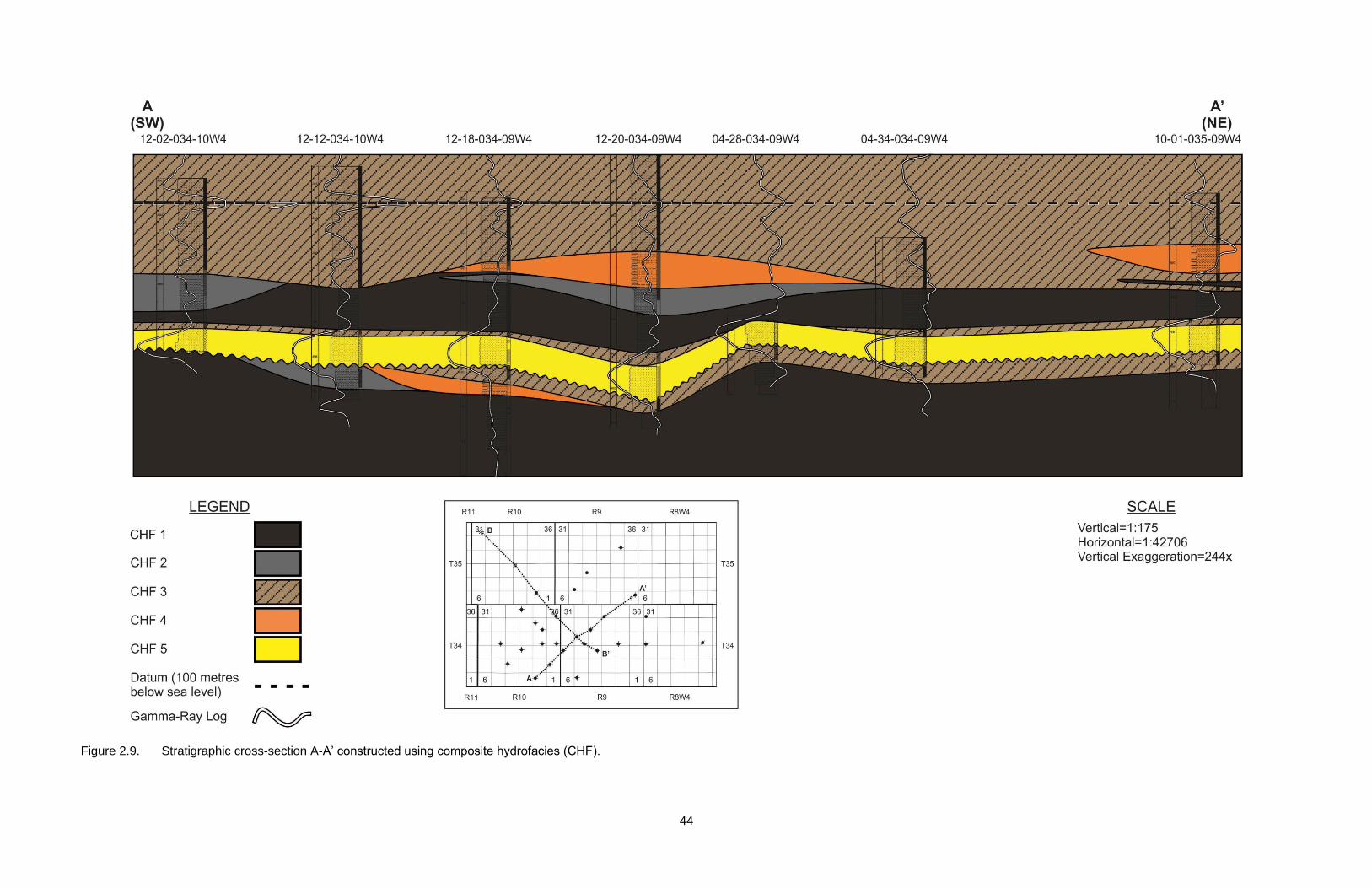
44
Figure 2.9. Stratigraphic cross-section A-A’ constructed using composite hydrofacies (CHF).

45
Figure 2.10. Stratigraphic cross-section B-B’ constructed using composite hydrofacies (CHF).

46
46
Chapter 3. Statistical Modeling of Biogenically Enhanced Permeability in Tight Reservoir Rock
This chapter has been published as Hsieh, A.I., Allen, D.M., and MacEachern,
J.A., 2015. Statistical modelling of biogenically enhanced permeability in tight
reservoir rock. Journal of Marine and Petroleum Geology 65, 114-125.
3.1. Introduction
The storage capacity and productivity of a reservoir are determined by its porosity and
permeability. Permeability is also an important factor that controls reservoir response during
enhanced recovery. Correspondingly, understanding and projecting variations in porosity and
permeability within a reservoir are vital to maximizing the acquisition of the resource. Recently,
there has been considerable interest in recovering hydrocarbons from marginal (generally
lower-quality) reservoirs using horizontal drilling techniques and fracturing, particularly in areas
prone to light oil. The so-called “Tight Oil” play of the Viking Formation in east-central Alberta
and west-central Saskatchewan is one example. “Tight” reservoirs are characterized by
permeabilities that range from 0.01-0.1 mD (Spencer, 1989; Holditch, 2006; Clarkson and
Pedersen, 2010). In such reservoirs, subtle changes in the distribution of sedimentary media,
such as are generated by bioturbation, can greatly affect the porosity and permeability
distribution of the facies (e.g., Gingras et al., 1999; Pemberton and Gingras, 2005; Gingras et
al., 2007; Tonkin et al., 2010; Baniak et al., 2012).
Bioturbation remains an under-appreciated mechanism by which porosity and
permeability of a sedimentary facies are modified (cf. Pemberton and Gingras, 2005). Even
when considered, bioturbation is generally perceived to be detrimental to bulk permeability,
through reduction of primary grain sorting, homogenization of the sediment, and introduction of
47
mud through linings, biogenic deposits, and feces (Qi, 1998; Dornbos et al., 2000; Qi et al.,
2000; McDowell et al., 2001; Pemberton and Gingras, 2005; Tonkin et al., 2010; Lemiski et al.,
2011; La Croix et al., 2013). Recent studies have shown, however, that several ichnogenera
and their associated biogenic fabrics are capable of increasing a reservoir rock’s porosity and
permeability (Gingras et al., 2004; Pemberton and Gingras, 2005; Hovikoski et al., 2007;
Volkenborn et al., 2007; Cunningham et al., 2009; Tonkin et al., 2010; Lemiski et al., 2011;
Gingras et al., 2012; La Croix et al., 2013; Knaust, 2014). Ichnogenera that form branching
burrow networks can create flow pathways in otherwise less permeable units where the burrow
fills consist of coarser grains and better-connected intergranular pore space relative to the
surrounding matrix (Figure 3.1; Gingras et al., 2004; Pemberton and Gingras, 2005; Lemiski et
al., 2011; Gingras et al., 2012; La Croix et al., 2013). Additionally, burrows are capable of
increasing vertical permeability in laminated sedimentary rocks, where horizontal permeability
otherwise tends to dominate (Gingras et al., 2012). Burrow fills also may undergo diagenetic
changes that may lead to higher permeability than that of the surrounding matrix (Pemberton
and Gingras, 2005; Tonkin et al., 2010; Gingras et al., 2012).

48
Figure 3.1. Sand-filled trace fossils such as Thalassinoides (Th) and Planolites (Pl) create potential flow paths in an otherwise low-permeability unit. Mud-filled traces are dominated by Phycosiphon (Ph).
Despite this, permeability across unfractured sedimentary reservoirs is commonly
assessed solely on the basis of grain size (e.g. lithostratigraphic units). By contrast, this paper
proposes the use of “hydrofacies” (HF) in reservoir characterization. A hydrofacies is defined
herein as a recurring sedimentary facies possessing a distinct permeability grade generated by
a combination of sedimentological and ichnological characteristics. Such a hydrofacies takes
into account the lithology, textural characteristics, physical and biogenic fabric, the presence
and distribution of trace fossils, and the expression of burrow fill(s), all of which serve to affect
permeable flow pathways (vertically and laterally) in heterolithic facies. The Markov chain
approach proposed in this paper is used to compare vertical transitions in permeability within a
borehole with transitions in a) grain size, and b) hydrofacies at the bed to bedset scale, in order
to determine which variable best reflects the observed permeability variations.

49
3.2. Geologic Setting
The Lower Cretaceous (Upper Albian) Viking Formation is a prolific oil- and gas-
producing interval that was deposited in the Western Canada foreland basin during a period of
active tectonism and eustatic sea level fluctuations. During Viking deposition, a shallow
epicontinental seaway extended from the Arctic Ocean to the Gulf of Mexico (Figure 3.2;
Williams and Stelck, 1975; Caldwell, 1984; Walker, 1990; Reinson et al., 1994), into which was
deposited a complex succession of siliciclastics, dominated by mudstones, heterolithic bedsets
of sandstone and shale, and sandstones, with minor conglomerates.
Figure 3.2. Map showing the major hydrocarbon-producing fields of the Viking Formation in Alberta (MacEachern et al., 1999).
The Viking Formation stratigraphically overlies the Joli Fou Formation and underlies the
Westgate Formation (Figure 3.3; Stelck, 1958). It is generally regarded to be roughly equivalent
to the Paddy Member of the Peace River Formation of northwestern Alberta (Leckie et al.,
1990), and the Bow Island Formation of southern Alberta and southwestern Saskatchewan

50
(Figure 3.3; Stelck and Koke, 1987; Raychaudhuri and Pemberton, 1992). Whereas the Viking
sediments only range from 15 to 30 m in thickness, they are discontinuity bound and
depositionally complex, resulting in sedimentary successions, facies, and geometries that are
challenging to characterize and correlate (e.g. Pattison, 1991; Reinson et al., 1994; Walker,
1995; Burton and Walker, 1999).
Figure 3.3. Stratigraphic correlation diagram of the Viking Formation in central Alberta showing the overlying Westgate Formation, underlying Joli Fou Formation, as well as its stratigraphic equivalents, the Paddy Member and Bow Island Formation (MacEachern et al., 1999).
The Late Albian (Lower Cretaceous) Viking Formation comprises a siliciclastic
succession consisting of interstratified mudstones, sandstones and rare conglomerates, mainly
reflecting shoreface, delta and estuarine valley deposits. These clastic sediments were
supplied from the rising Cordillera in the west and reflect northward and eastward progradation
of environments into the Alberta foreland basin. The Viking Formation overlies marine shale of
the Joli Fou Formation and is capped by marine shale of the Westgate Formation (Figure 3.3).
The stratigraphic relationships were addressed by the work of Stelck (1958), Glaister (1959),

51
McGookey et al. (1972), Weimer (1984), Cobban and Kennedy (1989), Stelck and Leckie
(1990), Bloch et al. (1993), Caldwell et al. (1993), and Obradovich (1993).
The Viking Formation is internally complex stratigraphically, and characterized by
numerous internal discontinuities. Beaumont (1984), Boreen and Walker (1991), Pattison
(1991), Posamentier and Chamberlain (1993), Reinson et al. (1994), Walker (1995), Burton and
Walker (1999), and MacEachern et al. (1999), among others, have attempted to provide
allostratigraphic and sequence stratigraphic assessments of the Viking, with varying levels of
success. Viking Formation discontinuities have been linked to the global changes of sea level
outlined in Kauffman (1977), Vail et al. (1977), Weimer (1984), and Haq et al. (1987). A cored
interval of the Viking Formation from the Verger Field was selected for this study because it
exhibits stacked parasequences characterized by the interstratification of impermeable and
permeable beds with variable but locally pervasive bioturbation.
3.3. Geostatistics
In this study, the transition probability method is used to model bioturbated,
heterogeneous sedimentary media. The transition probability method is a modified form of
indicator kriging that assumes the type of sediment that will be deposited in a stratigraphic
succession depends solely upon what is currently being deposited in the present environment
and not on the rock types deposited in past environments (Jones et al., 2002). For example, in
a prograding shoreface environment, one would expect to find a gradual upward-coarsening
succession of facies. If the rock type observed is fine-grained parallel laminated sandstone of
the middle shoreface, the next unit to be deposited is more likely to be coarser-grained cross-
stratified sandstone of the upper shoreface, regardless of what rock type was deposited before
the fine-grained parallel laminated sandstone. In terms of spatial distributions, the probability of
the occurrence of a class is dependent on the nearest occurrence of another class over a
specified lag interval. The probability of class 1 passing into class 2 can be defined by:
𝑝12ℎΦ = 𝑃𝑟{(𝑐𝑙𝑎𝑠𝑠 2 𝑜𝑐𝑐𝑢𝑟𝑠 𝑎𝑡 𝑥 + ℎΦ)|(𝑐𝑙𝑎𝑠𝑠 1 𝑜𝑐𝑐𝑢𝑟𝑠 𝑎𝑡 𝑥)} (3.1)
where ℎΦ represents the lag distance in the direction Φ (Carle, 1999).

52
The spatial correlation among different sedimentary facies can be calculated using a
Markov chain analysis; a mathematical model that transitions from one state to another between
a fixed number of possible discrete states (Carle, 1999). For example, a succession of
sedimentary facies may be characterized by a preferred tendency for sediment A to be
deposited after sediment B, but not sediment C; therefore, the spatial occurrence of sediment A
may be dependent on the pre-existence of sediment B but independent of sediment C (Li et al.,
2005). Additionally, if sediments A, B, and C tend to be deposited upwards as a sequence
ABC, this asymmetric relationship also can be characterized using Markov chain analysis (Li et
al., 2005).
The Markov chain is described as follows: There is a set of classes, S = {s1, s2, …, sr},
which pass sequentially from one to another in steps. The probability of class s1 moving to
class s2 is represented by p12, otherwise known as the transitional probability from s1 to s2. If
the transition remains in the same class s1, it is denoted by the probability p11 (Grinstead and
Snell, 1997). For example, Carle (1999) assessed the transition probabilities down a well log
using an embedded analysis of the Markov chain with respect to a matrix of vertical transitions
from one discrete sedimentary facies to another. In that study, an embedded Markov chain
analysis of a vertical succession was defined by three facies (A, B, and C) according to the
following steps (Carle, 1999):
1. Disregard the lag or spatial dependency and relative thicknesses of the beds.
2. Log the embedded occurrences of A, B, and C down the borehole (e.g. ABCABACABCABABC).
3. Count the number of transitions from one state to another in a transition count matrix.
A B C
A - 5 1
B 2 - 3
C 3 0 -
Self-transitions (e.g. from A to A) are unobservable in single or stacked beds, and are therefore null in the transition matrix.

53
4. Divide each transition count by the sum of the row, in order to find the embedded
transition probabilities.
A B C
A - 0.833 0.167
B 0.4 - 0.6
C 1 0 -
This final matrix shows the transition probabilities for each combination of units.
The Markov transition probability approach is generally useful for stratigraphically
confined systems. As is clear from Walther’s Law, genetic and predictable relationships exist
for facies successions that occur between stratigraphic breaks, which are absent in facies
separated by such breaks. Markov transition probability can be used to demonstrate the lack of
correlatibility of facies across such stratigraphic breaks (Weissmann, 2005). Another advantage
of using Markov chain models is that the approach assumes stratigraphic stationarity (statistical
homogeneity; i.e. the mean and standard deviation do not change over time or space) across
the modeled reservoir (Weissmann, 2005). In other words, by dividing the core into facies, the
proportions and geometries of different facies within the environment are maintained. In a
transgressive marine environment, for example, the proportion of fine-grained facies is higher
than coarse-grained facies across the environment, and the probability of fine-grained facies
being deposited is likewise greater. This ensures that a facies represented in the model is not a
result of random variables, but rather is reflective of the character of the depositional conditions.
Furthermore, the distribution of facies within the stratigraphic unit theoretically can be simulated,
resulting in a quantifiable conceptual model that facilitates the interpretation of the reservoir’s
heterogeneity (Weissmann, 2005).
3.4. Methodology
3.4.1. Core Logging
Well 14-30-22-16W4 in the Verger Field contains core through the Viking Formation, and
was selected for this study because it exhibits the interlayering of impermeable and permeable
beds (e.g. mudstones and sandstones) that are thoroughly bioturbated in certain sections. All of

54
the physical and biogenic features observed in the core, including lithology, grain size,
bioturbation index (BI) and ichnological suites, were logged from the base to the top of the well
using AppleCORE, a core-logging program that allows the user to record descriptive geological
data and convert the data into a strip log (Figure 3.6).
3.4.2. Permeability Data
The permeability data for the well were obtained from AccuMap, an oil and gas mapping,
data management and analysis software for companies operating in the Western Canadian
Sedimentary Basin and Frontier areas (AccuMap IHS; accessed 06 February, 2013). The
AccuMap data for well 14-30-22-16W4 include 44 horizontal permeability (kmax) values that were
measured at discrete locations over the length of the core. Each kmax value was measured
using both plug and full diameter samples from the core. At the bed/bedset scale, an average
kmax value was calculated from the raw permeability data to represent each HF as described
below. For the transition probability analysis, the kmax values were classed by increasing
magnitudes in logarithmic scale (0.01, 0.1, 1, 10, and 100 mD) to enable comparison firstly
between permeability and grain size, and secondly between permeability and HF.
3.4.3. Hydrofacies and Parameter Class Divisions
Hydrofacies (HF) were qualitatively defined at the bed/bedset scale based on distinct
sedimentary, ichnological, and potential permeability attributes. The average grain sizes
observed in the core were divided according to the Wentworth (1922) grain-size classification
scale: clay, silt, lower fine-grained sand, upper fine-grained sand, and lower medium-grained
sand. Bioturbation index (BI) reflects grades of bioturbation intensity, and were assigned values
from 0 to 6, with 0 being unburrowed, and 6 being the most intensely burrowed (Figure 3.4;
Reineck, 1963; Taylor and Goldring, 1993; Taylor et al., 2003). BI values of 6 (complete
bioturbation) were not observed in the cored interval.

55
Figure 3.4. Schematic diagram of the bioturbation index (BI), modified from Reineck (1963), Taylor and Goldring (1993) and Taylor et al. (2003) by MacEachern and Bann (2008). Bioturbation grades correspond to: BI 0 = 0% bioturbation; BI 1 = 1-4% bioturbation; BI 2 = 5-30% bioturbation; BI 3 = 31-60% bioturbation; BI 4 = 61-90% bioturbation; BI 5 = 91-99% bioturbation; and BI 6 = 100%.
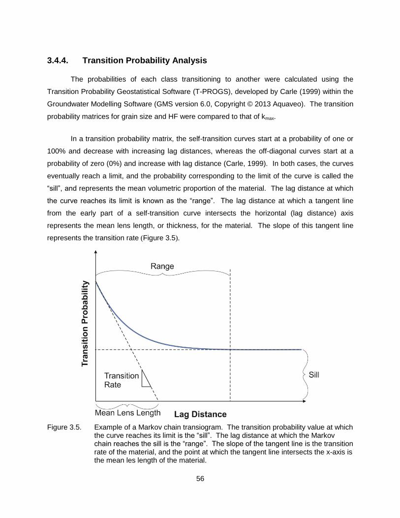
56
3.4.4. Transition Probability Analysis
The probabilities of each class transitioning to another were calculated using the
Transition Probability Geostatistical Software (T-PROGS), developed by Carle (1999) within the
Groundwater Modelling Software (GMS version 6.0, Copyright © 2013 Aquaveo). The transition
probability matrices for grain size and HF were compared to that of kmax.
In a transition probability matrix, the self-transition curves start at a probability of one or
100% and decrease with increasing lag distances, whereas the off-diagonal curves start at a
probability of zero (0%) and increase with lag distance (Carle, 1999). In both cases, the curves
eventually reach a limit, and the probability corresponding to the limit of the curve is called the
“sill”, and represents the mean volumetric proportion of the material. The lag distance at which
the curve reaches its limit is known as the “range”. The lag distance at which a tangent line
from the early part of a self-transition curve intersects the horizontal (lag distance) axis
represents the mean lens length, or thickness, for the material. The slope of this tangent line
represents the transition rate (Figure 3.5).
Figure 3.5. Example of a Markov chain transiogram. The transition probability value at which the curve reaches its limit is the “sill”. The lag distance at which the Markov chain reaches the sill is the “range”. The slope of the tangent line is the transition rate of the material, and the point at which the tangent line intersects the x-axis is the mean les length of the material.

57
3.5. Results and Discussion
3.5.1. Hydrofacies
Five hydrofacies were identified at the bed/bedset scale in the studied core (Table 3.1):
bioturbated/non-bioturbated mudstone; bioturbated silty mudstone; bioturbated muddy
sandstone; bioturbated sandstone; and sandstone. For the logged core, only plug permeability
data were available for HF 4 and 5, and only full-diameter core permeability data were available
for HF 2 and 3. The plug and full-diameter core analyses capture permeability at different
scales. The plug permeability represents k at the bed scale, whereas full-diameter permeability
analyses capture bulk permeability. In heterogeneous units, for example, the plug permeability
may be biased towards coarser-grained more permeable units, while full diameter analyses
capture the permeability of both coarse- and fine-grained units and is more representative of the
overall permeability. Due to the paucity of data, however, the plug and full diameter
permeability measurements are assumed to be equivalent. Additionally, because the plug
samples only measure kmax in the horizontal direction, the horizontal kmax measured in the full
diameter samples were used instead of vertical k. The average permeability (kave) is calculated
for HF 2, 3, and 5. For HF 4, only one permeability measurement was available, so that value
(kmax) is assumed to be representative for all HF 4 at the bed/bedset scale. Permeability was
not measured for any of the mudstone hydrofacies (HF 1); therefore, the geometric mean
(geomean) of the range of mudstone permeabilities measured in other studies was used (e.g.
Mesri and Olson, 1971; Long, 1979; Long and Hobbs, 1979; Nagaraj et al., 1994; Dewhurst et
al., 1998, 1999; Yang and Aplin, 2007, 2010). Table 3.1 reports the average or representative k
values for each HF.

58
Table 3.1. Bed/bedset scale hydrofacies descriptions. The calculated kave (mD) or representative kave based on previous studies for each HF are also reported.
Hydrofacies Lithology Grain Size Sedimentary Structures BI Trace Fossils (in approximate order of decreasing abundance)
kave (mD)
1 Apparently structureless mudstone
Mudstone Clay Apparently structureless, sharp-based mudstone
Apparently low (BI 0-1) or high (BI 4-5) if bioturbation is present and observable
Rare Chondrites and Planolites 1.31E-04a
2 Bioturbated silty mudstone
Mudstone with moderate proportions of interstitial silt and sand
Lower to upper silt
No sedimentary structures observed
4-5 Phycosiphon, Chondrites, Helminthopsis, Planolites, Asterosoma, Schaubcylindrichnus, Thalassinoides, Teichichnus, Zoophycos, Diplocraterion, with rare Rosselia and fugichnia
0.35
3 Bioturbated muddy sandstone
Sandstone with moderate proportions of interstitial silt and clay
Lower fine- to upper fine-grained sand
No sedimentary structures observed
3-5 Phycosiphon, Chondrites, Helminthopsis, Planolites, Asterosoma, Teichichnus, Schaubcylindrichnus, Zoophycos, Thalassinoides, Palaeophycus, Diplocraterion, Skolithos, Ophiomorpha, Rosselia, Rhizocorallium and fugichnia 1.24
4 Bioturbated sandstone
Sandstone Lower fine- to upper fine-grained sand
Apparently structureless 4-5 Phycosiphon, Asterosoma, and fugichnia
5.03b
5 Sandstone Sandstone Lower fine- to upper fine-grained sand
HCS or horizontal to low-angle (5°) planar parallel laminated or wave ripple laminated, sharp-based
0 Not observed
4.20
a Calculated geometric mean of values from the literature
b Only one value available for the core

59
Figure 3.6. Core log of PCP Verger 14-30-22-16W4.

60
HF 1 encompasses apparently structureless, sharp-based mudstones (Figure
3.7). Bioturbation may appear absent (BI 0-1) owing to a homogeneously muddy matrix,
but where interstitial silt and sand contents are slightly higher or burrows reflect sand or
silt segregation from the matrix, bioturbation intensities may range from 4-5. Trace
fossils in HF 1 include rare Chondrites and Planolites. The kave calculated from previous
work is 1.31E-04 mD (cf. Mesri and Olson, 1971; Long, 1979; Long and Hobbs, 1979;
Nagaraj et al., 1994; Dewhurst et al., 1998, 1999; Yang and Aplin, 2007, 2010).
HF 2 corresponds to bioturbated silty mudstone with moderate proportions of
interstitial silt and sand (Figure 3.7). Primary stratification is not preserved. Bioturbation
intensities are high (BI 4-5) with a diverse trace-fossil suite consisting of Phycosiphon,
Chondrites, Helminthopsis, Planolites, Asterosoma, Schaubcylindrichnus,
Thalassinoides, Teichichnus, Zoophycos, Diplocraterion, with rare Rosselia and
fugichnia, in order of approximate decreasing abundance. The kave value for HF 2 is
0.35 mD.
HF 3 is characterized by bioturbated muddy sandstones with moderate
proportions of interstitial silt and clay (Figure 3.7). No primary sedimentary structures
are preserved in HF 3 due to the high bioturbation intensities (BI 3-5). The diverse
trace-fossil suite, in order of approximate decreasing abundance, comprises
Phycosiphon, Chondrites, Helminthopsis, Planolites, Asterosoma, Teichichnus,
Schaubcylindrichnus, Zoophycos, Thalassinoides, Palaeophycus, Diplocraterion,
Skolithos, Ophiomorpha, Rosselia, Rhizocorallium and fugichnia. The kave value for HF
3 is 1.24 mD.
HF 4 consists of sandstones with rare preserved primary sedimentary structures
due to bioturbation (Figure 3.7). Bioturbation intensities range from BI 4-5, and the
trace-fossil suite includes isolated Phycosiphon, Asterosoma, and fugichnia. The
representative k value for HF 4 is 5.03 mD.
HF 5 is composed of unburrowed (BI 0), well-sorted sandstones that are
hummocky cross-stratified, horizontal to low-angle (5°) planar parallel laminated, or
wave-ripple laminated (Figure 3.7). The kave value for HF 5 is 4.20 mD.

61

62
Figure 3.7. Examples of hydrofacies. A) Hydrofacies (HF) 3, 4, and 5 with Phycosiphon (Ph), Planolites (P), Scolicia (Sc), Asterosoma (As), and Schaubcylindrichnus (Sch). HF 5 exhibits planar parallel laminae. B) HF 2 with Chondrites (Ch), Asterosoma (As), and Phycosiphon (Ph) interbedded with laminated HF 4 containing Asterosoma (As) and fugichnia (fu). C) Wave ripple laminated HF 5 overlying HF 3 and HF 1. Trace fossils in HF 3 include Phycosiphon (Ph) and Schaubcylindrichnus (Sch). D) HF 5 and HF 4 interbedded with HF 1. Trace fossils in HF 4 include Asterosoma (As) and Phycosiphon (Ph). Trace fossils in HF 1 include Planolites (P) and Chondrites (Ch).
3.5.2. Transition Probability (Markov Chain) Analyses
The transition probability matrices are shown in Figure 3.8 for grain size vs. kmax
and in Figure 3.9 for HF vs. kmax. The transitions from class 1 to 2 are read from rows to
columns. The dominant control on permeability should have similar transition probability
curves as kmax. The Markov chains for grain size (Figure 3.8) show similar transition
probability trends only in column 1 and column 5. Units with clay-sized grains typically
appear structureless, and mud-filled trace fossils dominate the trace-fossil suite
observed within these units. Units dominated by lower medium (mL)-grained sandstone
typically lack bioturbation, and are structureless or laminated. This suggests that grain
size only influences permeability where the rock units are relatively homogeneous,
whereas intermediate permeabilities (i.e., 0.1-10 mD) are controlled by a number of
variables captured by the hydrofacies. The kmax values were classed for the transition
probability analyses to enable comparison of the two approaches.
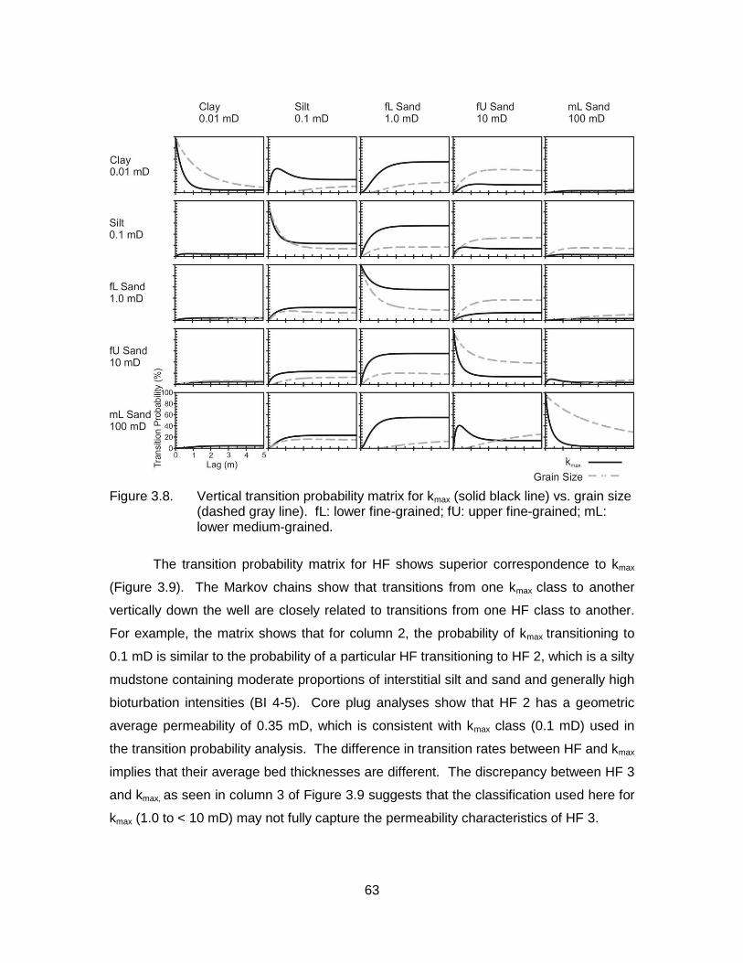
63
Figure 3.8. Vertical transition probability matrix for kmax (solid black line) vs. grain size (dashed gray line). fL: lower fine-grained; fU: upper fine-grained; mL: lower medium-grained.
The transition probability matrix for HF shows superior correspondence to kmax
(Figure 3.9). The Markov chains show that transitions from one kmax class to another
vertically down the well are closely related to transitions from one HF class to another.
For example, the matrix shows that for column 2, the probability of kmax transitioning to
0.1 mD is similar to the probability of a particular HF transitioning to HF 2, which is a silty
mudstone containing moderate proportions of interstitial silt and sand and generally high
bioturbation intensities (BI 4-5). Core plug analyses show that HF 2 has a geometric
average permeability of 0.35 mD, which is consistent with kmax class (0.1 mD) used in
the transition probability analysis. The difference in transition rates between HF and kmax
implies that their average bed thicknesses are different. The discrepancy between HF 3
and kmax, as seen in column 3 of Figure 3.9 suggests that the classification used here for
kmax (1.0 to < 10 mD) may not fully capture the permeability characteristics of HF 3.

64
Figure 3.9. Vertical transition probability matrix for kmax (solid black line) vs. hydrofacies (dotted gray line).
The results of the Markov transition probability were also analyzed for correlation.
A correlation of +100% indicates a perfect direct relationship between two variables, and
a correlation of -100% indicates a perfect inverse relationship. A correlation of zero
indicates a lack of correlation (Davis, 1986). The Markov chains show that the
volumetric proportions, as indicated by the sill values of different kmax classes, correlate
with grain size by 15%, even though it is commonly assumed that grain size and
permeability have a high, positive correlation (coarse grain sizes being associated with
high permeability). However, permeability correlates with the established hydrofacies by
97%, indicating that variations in permeability down the well are strongly related to
variations in the HF.

65
3.6. Conclusions
The results from the transition probability analyses show that horizontal
permeability does not correlate well with conventional grain size classifications alone,
suggesting that permeability is controlled by additional factors, such as sedimentary
structures, bioturbation, and sedimentary accessories. In the studied core intervals,
bioturbation plays an important role in the creation and alteration of permeable flow
paths within these fine-grained units by generating sand-filled burrows and destroying
primary sedimentary structures. Therefore, in order to show a consistent correlation
between rock type and permeability, it is important to characterize the rock on the basis
of all of its physical, chemical, biogenic, and hydraulic properties by defining the
hydrofacies. These hydrofacies show a clear and quantifiable relationship to
permeability in the vertical direction. The results show that in the studied well, grain size
only correlates closely to permeability in homogeneous, very coarse- or very fine-grained
rock units such as sandstone (HF 5) or mudstone (HF 1). In contrast, the transiograms
for HF show similar sill values with kmax, indicating that the two attributes have
comparable volumetric proportions within the cored interval. Nevertheless, the
difference in transition rates between HF and kmax indicates that their average bed
thicknesses are different.
The T-PROGS software used for the transition probability calculations limits the
geologic data to a maximum of five different classes, which may be insufficient to
adequately represent some geologically complex reservoirs. Other limitations to this
study include the small number of permeability values for the studied cored interval.
Only horizontal kmax values were available for the transition probability analysis.
Additionally, permeability measurements are historically only conducted on the coarsest-
grained units, despite the fact that these facies types may not be representative of the
dominant flow unit in tight reservoirs. The paucity of permeability analyses in muddy or
strongly heterolithic bedsets limits the applicability of statistical analyses.
Micropermeametry may be used to refine the kave of each HF, as it measures detailed
and precise permeability at the centimetre scale. Nonetheless, the approach for defining
hydrofacies is directly applicable to all low-permeability reservoirs, wherein grain size
may not be the dominant factor but rather only one of many controls on permeability

66
distributions. This approach can potentially be used as a conceptual framework for the
spatial modeling of permeability in low-permeability reservoirs.

67
Chapter 4. Upscaling Permeability for Regional Flow Modeling
4.1. Average Hydraulic Conductivity for Bed to Bedset Scale HFs
As discussed in Chapter 2, five discrete and recurring composite hydrofacies
(CHFs) were identified in 28 wells of the Viking Formation from the Provost Field. These
are composed of varying proportions of five bed/bedset scale hydrofacies (HFs) defined
in Chapter 3, but with different geometric average permeabilities as shown in Table 4.1.
The average permeability (mD) calculated for these bed/bedset scale hydrofacies were
converteda to average hydraulic conductivity (Kave in m/s) for flow modeling.
Table 4.1. Bed/bedset scale hydrofacies identified in core and the calculated average hydraulic conductivity (Kave) in m/s or representative Kave based on previous studies for HF 1. Kave values calculated in Chapter 3 are also shown below.
HF: bed/bedset Ch. 3 Kave (m/s) Kave (m/s)
1* Apparently structureless mudstone/siltstone
1.2610-12 1.2610-12
2 Bioturbated silty mudstone 3.3710-09 7.1410-09
3 Bioturbated muddy
sandstone
1.1910-08 3.0610-08
4 Bioturbated sandstone 4.8410-08 7.9810-07
5 Sandstone 4.0410-08 1.2710-06
* The average hydraulic conductivity for
HF a was calculated from Mesri and Olson (1971), Long
(1979), Long and Hobbs (1979), Nagaraj et al. (1994), Dewhurst et al. (1998, 1999), and Yang and Aplin (2007, 2010).
a 1 Darcy equals 0.831 m/day under hydrostatic pressure of 0.1 bar/m at a temperature of 20ºC (Duggal and Soni, 1996).

68
4.2. Hydraulic Conductivity Estimation for Composite HFs
The bed/bedset scale HFs are on the order of centimetres thick – a scale that is
impractical to capture at the reservoir scale. Therefore, upscaling of the permeability is
required. To do this, the cores were re-logged according to composite HFs (CHFs, see
Chapter 2), and an upscaled equivalent K estimated for each CHF. The equivalent K
represents the thickness-weighted sum of Kave of the bed/bedset scale HFs comprising
the CHF. The equivalent K values were calculated for each CHF in both the horizontal
(Kh) and vertical (Kv) directions using the following expressions for layered media
(Freeze and Cherry, 1979; Figure 4.1):
Figure 4.1. Upscaling hydraulic conductivity (K) at the bed to bedset scale to a single equivalent hydraulic conductivity in both the vertical (Kv) and horizontal (Kh) directions for a composite hydrofacies using the expressions for layered media (see Equations 4.1 and 4.2).
𝐾ℎ = ∑𝐾𝑎𝑣𝑒𝑚𝑏𝑚
𝑏
𝑛𝑚=1 (4.1)
𝐾𝑣 =𝑏
∑𝑏𝑚
𝐾𝑎𝑣𝑒𝑚
𝑛𝑚=1
(4.2)

69
where m is the particular bed/bedset scale HF, b is the total thickness of the CHF, Kavem
is the average hydraulic conductivity measured from plug samples for a particular
bed/bedset scale HF, and bm is the thickness of individual beds (cf. Freeze and Cherry,
1979). As only horizontal permeability measurements were available from plug samples,
it was assumed that the bed from which the plugs were taken are isotropic at the plug
scale. Equations 4.1 and 4.2 likewise assume that each layer is isotropic and
homogeneous (Freeze and Cherry, 1979).
4.3. Validation of Equivalent K
To test the equivalency of the Kh and Kv values assigned to the CHF against
those of the layered bed/bedset HFs system, a series of steady state, two-dimensional
numerical flow models were run. Each block model corresponds to an interval of core
that represents a single CHF. The CHF is, in turn, made up of bed/bedset scale HFs.
First, for each block model, a horizontal and a vertical flow simulation were run over the
width and length of the core, respectively. The models were first run using the Kave for
the individual bed/bedset scale HFs that constitute the section of core. Following that,
the models were run again over the same section of core, but using a single Kh or Kv for
the CHF. The models were constructed in the modeling software Visual MODFLOW, a
three-dimensional, finite-difference, block-centred groundwater flow model (Version
2011.1, © Schlumberger Water Services).
For the block models, the x direction represents the diameter of the core (10 cm),
and the y direction represents length (vertical height) of the CHF (Figure 4.2). As
MODFLOW only accepts integers for defining the model domain, the length and
diameter of the cored sections were scaled up by 100. Thus, the resulting dimensions
of the models extend 10 m in the x direction, and vary in the y direction depending on
the length of the CHF. A 1 x 1 m grid spacing was used. A single model layer of unit
thickness in the z direction was used because only the vertical (y direction) and
horizontal (x direction) flow were simulated. Thus, the models are essentially two-
dimensional.

70
For horizontal flow simulations, the left and right boundaries were assigned
specified head values of 10 m and 9 m (Figure 4.2 A), whereas the top and bottom of the
model were no flow boundaries. To generate a flow field for the vertical flow simulations,
the top and base of the model were assigned specified head values of 10 m and 9 m,
respectively (Figure 4.2 B). Thus, depending on the length of each model, the hydraulic
gradient was differentb. The left and right margins were assigned as no flow boundaries.
No other boundary conditions were applied.
.
Figure 4.2. Boundary conditions for A) horizontal flow simulations and B) vertical flow simulations. h refers to the assigned hydraulic head.
b The hydraulic gradient is defined as the difference in head (here, 10 – 9 m) divided by the vertical separation (here, the length of the composite HF for vertical flow simulations).

71
The only assigned property was hydraulic conductivity, which varies as described
below. Other parameter values in Visual MODFLOW are not needed for steady state
flow simulations.
As mentioned above, for each interval of core, two separate steady state models
were run: one at the bed/bedset scale and one at the composite scale (Figure 4.3).
1. First, flow was simulated using the hydraulic conductivities of the individual
beds/bedsets that comprise the interval of core.
a) A vertical flow field was generated. This vertical flow depends only on
the K values of the stacked sequence and the vertical hydraulic gradient.
The hydraulic gradient varies according to the height of the core. Each
layer (bed) has an isotropic and homogeneous K of magnitude Kave
corresponding to the respective HF.
b) Next, a horizontal flow field was generated. This horizontal flow depends
on the hydraulic conductivities of layers. The hydraulic gradient is
uniform for all models, owing to the same core widths.
2. Simulations were then run over the same interval of core at the composite
scale using each equivalent hydraulic conductivity that represents the section
(Kh or Kv).
3. The discharge (Q in m3/s) from 1) and 2) were compared to verify that flow
through a heterogeneous, bioturbated unit is the same as that through the CHF
in each direction.
4. The resulting horizontal and vertical discharges for the composite scale
simulations were grouped according to CHF, and average horizontal and
vertical discharges (Q) were calculated for each.
5. Average hydraulic conductivity values in the horizontal and vertical direction
were then calculated for each of the five CHFs using the average horizontal
and vertical discharge (from step 4), according to the following equation:
K = −𝑄
𝐴×
𝑑ℎ
𝑑𝑙 (4.3)
where K is the hydraulic conductivity, Q is the discharge, A is the cross-sectional area perpendicular to the flow direction, and dh/dl is the hydraulic gradient (Darcy, 1856). This final step was to confirm that any numerical errors did not affect the results. If the calculated K was the same as the equivalent K in the respective direction, then the simulations were considered robust.
In addition, the water balance was calculated for each simulation to confirm that
mass was conserved in the numerical simulation. Given the very small bed thicknesses

72
for some models and/or the low hydraulic conductivities of the muddier units, the solver
settings had to be carefully adjusted to assure water balance closure.
Figure 4.3. A) Example of a MODFLOW block model of a cored section with hydrofacies logged at the bed/bedset scale. Each colour represents a different hydrofacies. B) Block model of the same cored section with hydrofacies logged at the composite scale.
The results of the numerical block modeling showed that for the horizontal flow
models, the discharges Q (m3/s) for the bed/bedset HF and the CHFs had an average
discrepancy of 0.47%, disregarding one outlier value resulting from poor model
convergence (Figure 4.4A; Appendix C). For the vertical flow models, the average

73
discrepancy is 1.27% (Figure 4.4B; Appendix D), disregarding five outliers. In general,
a discrepancy less than 5% is considered acceptable, and simulations that yielded a
discrepancy greater than 5% were considered outliers (Anderson and Woessner, 1992).
This suggests that both vertical and horizontal flow through heterogeneous, bioturbated
media can be simplified using an upscaled equivalent K that represents the variability in
permeability at the bed/bedset scale.

74
Figure 4.4. Discharge in Q (m3/s) for bed/bedset scale and composite scale fluid flow simulations in the A) horizontal and B) vertical directions.
The average horizontal hydraulic conductivity (Kh) generally increases from CHF
1 to 5 (Table 4.2). The resulting average Kv, however, did not increase consistently.
CHF 3, though finer in average grain size than CHF 5, has a higher average Kv. CHF 3
is moderately to intensely bioturbated, and some of the bioturbation may serve to
generate vertical flow paths, thereby increasing overall vertical conductivity. Also, the

75
discrete and laterally continuous mudstone laminae/beds observed across some cored
sections of CHF 5 are potentially capable of decreasing vertical conductivity.
Table 4.2. Minimum, maximum, and average horizontal (Kh) and vertical (Kv) conductivities for each composite hydrofacies.
Composite HF
Min Kh
(m/s) Max Kh
(m/s) Avg Kh
(m/s) Min Kv
(m/s) Max Kv
(m/s) Avg Kv
(m/s)
1 1.2610-12 1.2510-07 7.1810-10 1.2610-12 3.7910-12 1.5010-12
2 1.2610-12 1.6110-08 7.7510-10 1.2610-12 2.6610-12 1.7610-12
3 8.0310-09 2.6410-07 7.3210-08 1.4710-12 3.6910-08 4.4210-11
4 9.7610-09 1.8110-07 6.6010-08 2.7610-12 1.4610-11 6.5510-12
5 7.0410-07 1.1310-06 9.5210-07 1.2310-11 8.9110-11 3.0410-11
4.4. Regional Flow Simulations
4.4.1. CHF Model Setup
A hydrogeological cross section along B-B’ was constructed to show the present-
day geological structures that control fluid migration (Figure 4.5). Section B-B’ is aligned
with the regional hydraulic gradient (as described below). For this cross section, the
datum is sea level, and each hydrofacies is correlated above or below the datum
according to its present-day position.

76
Figure 4.5. Hydrogeological cross-section B-B’ constructed using Composite Hydrofacies (CHF).

77
The regional hydraulic gradient of formation waters was estimated from the
regional-scale hydraulic head distribution map for the Viking Formation constructed
using approximately 3600 drill stem tests (Figure 4.6; Bachu et al., 2002). The hydraulic
heads vary from >800 m in the south and <600 m in the east to <300 m in the southwest
(Figure 4.6). Cross-section B-B’ intersects a trough, and has an estimated hydraulic
gradient that trends roughly SE to NW along the regional strike, parallel to the line of
section. The estimated SE-NW trending hydraulic gradient is an oversimplification of the
actual system. The hydraulic head contours shown in Figure 4.6 indicate that
groundwater flow actually converges from SE to NW. This suggests that the direction of
formation water flow is not solely controlled by the regional structural dip towards the
SW. In addition to topography, the flow of formation waters is driven by other
mechanisms, including compaction, tectonic compression, erosional rebound, and
buoyancy, several of which may be active in a basin at any given time (Bachu, 1999). In
the Viking Formation, the regional extent of underpressuring and the inward flow of
formation waters is driven by erosional rebound and gas zones in the deep basin (Bachu
et al., 2002).
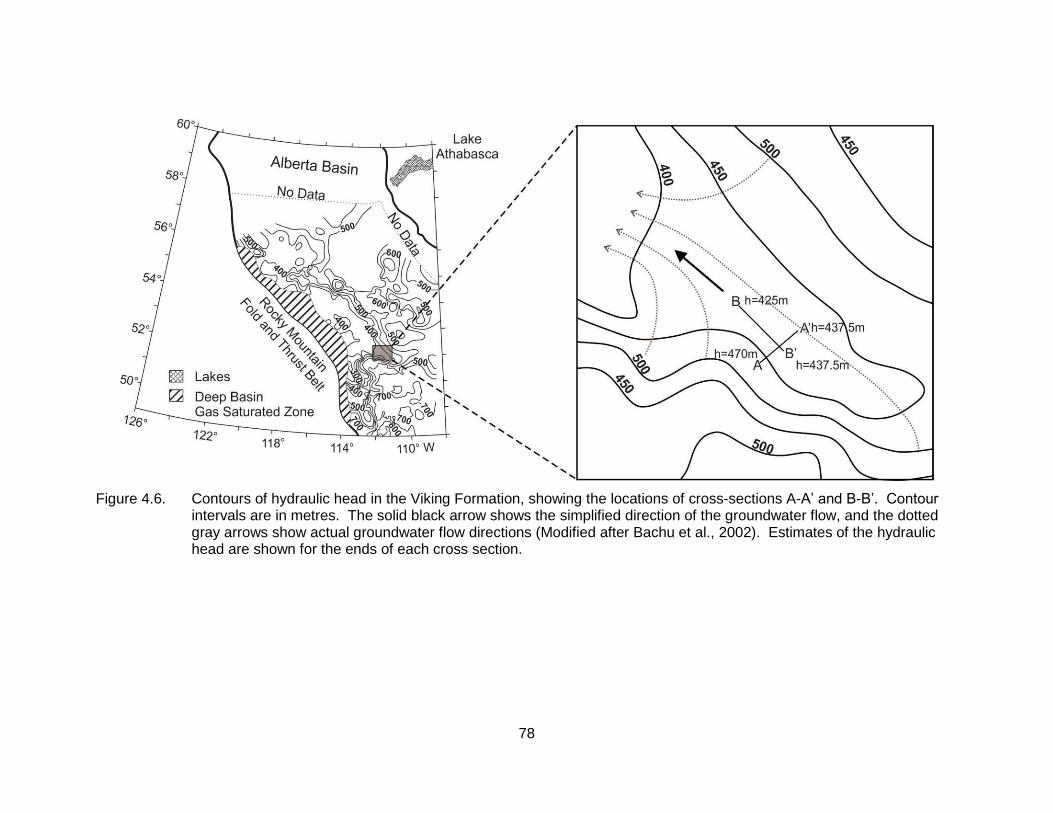
78
Figure 4.6. Contours of hydraulic head in the Viking Formation, showing the locations of cross-sections A-A’ and B-B’. Contour intervals are in metres. The solid black arrow shows the simplified direction of the groundwater flow, and the dotted gray arrows show actual groundwater flow directions (Modified after Bachu et al., 2002). Estimates of the hydraulic head are shown for the ends of each cross section.

79
The hydraulic gradient along cross-section B-B’ was estimated as follows:
𝑑ℎ
𝑑𝑙=
437.5 𝑚−425.0 𝑚
19.95 𝑘𝑚×1000 𝑚
𝑘𝑚
= 6.3 × 10⁻⁴ 𝑚/𝑚 (4.4)
where dh is the difference in hydraulic head from B to B’ (Figure 4.6) and dl is the length
of B-B’. Flow is roughly from SE to NW.
The hydrogeological cross section was reproduced in Visual MODFLOW by
visually transferring the contacts between CHFs (Figure 4.7). The model domain was
discretized to 250 x 100 m in the x and z directions, respectively. A single, 1 m model
layer in the y direction was used; thus was model was effectively two-dimensional. The
hydraulic conductivities assigned to the CHFs in the cross section are the average Kv
and Kh values for each CHF (refer to step 4 in Section 4.3).
The actual hydraulic head values at the NW and SE ends of the profile are 437.5
m and 425.0 m; however, because the base of the MODFLOW model is at 0 m rather
than -121.64 m below sea level, the specified head boundaries were adjusted to 1 m and
13.5 m, respectively. Thus, the hydraulic gradient remains the same (1 – 13.5 / 19950 m
= 6.3 x 10⁻⁴ as in Equation 4.4). It was assumed that only a horizontal gradient exists,
because no data for the vertical gradient are available. The specified head values were
assigned across the full vertical thickness of each end of the profile. The top and bottom
boundaries of the profile were assigned no flow boundaries. These no flow boundary
conditions assume that the flow is constrained to the units in the cross section and that
there is no transfer of formation water from this sequence to either an overlying or
underlying sequence of rocks, which is likely an oversimplification of the actual system
locally.
The model was run under steady-state conditions, and the water balance
calculated. The average fluid flux along the cross section was calculated using the
following equation:
𝑞 =𝑄
𝐴 (4.5)

80
where q is the flux (m/s), Q1 is the discharge (m3/s), and A is the cross-sectional area
(m2) of the profile (Freeze and Cherry, 1979). Q was estimated from the water balance
in Visual MODFLOW (flow exiting the model domain from the specified head boundary in
the NW), and A is the total thickness of the domain at that same end.
1 Q is a volumetric flow rate for groundwater moving along a hydraulic gradient; Q is not a production rate.

81
Figure 4.7. MODFLOW domain for hydrogeological cross-section B-B’ showing the hydraulic heads (h) at the NW and SE boundaries.

82
4.4.2. Additional Simulations Based on Literature K Values
Flow was also simulated along the line of section B-B’ using hydraulic
conductivity ranges for the Viking Formation as published in literature (Table 4.3). In
general, the hydraulic conductivity and Darcy flux measured by various sources
represent an average of fine- to medium-grained sandstones in the Viking Formation.
The measurements were taken from both drill stem tests and core analyses. Bekele et
al. (2002) measured maximum permeability parallel with bedding using 69,532 core
plugs from both sandstone and mudstone samples. BlackPearl Resources Inc. (2012)
performed a pumping test in a Viking Fm sandstone unit and obtained regional estimates
for such sandstones. Cao et al. (2014) estimated the permeability range based on low-
energy depositional environments such as delta-front, prodelta, tidal flat, or transitional
facies between shoreface and offshore facies (e.g., upper offshore regimes).

83
Table 4.3. Hydraulic conductivity (K) values of the Viking Formation measured in published literature, including the measurement techniques used as well as the lithology in which the measurements were taken.
K (m/s) Technique Lithology
Lerand and Thompson (1976) 1.6410-06 -------- Sandstone
Alho et al. (1977) 9.6210-08 to 1.4410-06 --------
Fine- to medium-grained sandstone
Bachu (1985) __ a Drill stem test (DST), core analyses Average of Viking sandstone
Bachu (1988) 1.5010-07 DST, core analyses Average of Viking sandstone
Bachu (1999) __ a DST, core analyses Average of Viking sandstone
Bekele et al. (2002) 9.6210-11 to 9.6210-05 (sandstone)
Core plug analyses Sandstone and shale 9.6210-15 to 9.6210-06 (shale)
Cenovus FCCL Ltd. (2009) Kh=1.0010-06, Kv=1.0010-08 DST Average of Viking aquifer
BlackPearl Resources Inc. (2012) 1.6010-07 to 6.0010-06 Regional estimates, pumping test Average of Viking aquifer
Matrix Solutions Inc. (2012) 2.0010‐07 to 7.0010‐06 DST, core analyses Average of Viking sandstone
Cao et al. (2014) 9.6210-10 to 9.6210-08
Estimates of deposits from low-energy environments such as delta-
front, prodelta, tidal flat, or transitional zone between shoreface and offshore
deposits
--------
a No hydraulic conductivity values were given. However, an estimated Darcy flux (q) in m/s is available.

84
Flow simulations were run using the K values reported for each study in Table
4.3. Where there is a range of K, two simulations were run using the lower limit and the
upper limit of the given range. For Bekele et al. (2002), CHFs 1-2 were assigned the K
for shale, and CHFs 3-5 were assigned the K for sandstone. Again, one simulation was
run using the lower limits of Ks for shale and sandstone, and another was run using the
upper limits of Ks. For Cenovus FCCL Ltd. (2009), the Kh and Kv were assigned to the
entire section. Darcy flux values were calculated for each model using the same
approach described in the previous section (Equation 4.5) and compared with the flux
calculated from the simulation using the average equivalent K calculated for the CHFs.
4.4.3. CHF Simulation Results
Groundwater flows from the SE boundary to the NW boundary, based on the
distribution of the equipotential contours generated from the model. The simulated flow
regime is consistent with the general regional groundwater flow of the Viking Formation
(Figure 4.8). The equipotential contours are relatively parallel throughout CHF 1, but
deviate through the CHFs with higher hydraulic conductivities (hydrofacies 3, 4, and 5).
This deviation in the equipotential contours is expected for flow through a heterogeneous
system and reflects the varying hydraulic conductivities across the section.

85
Figure 4.8. Equipotential head contour map of cross-section B-B’. Contour units are in metres. The zoomed section illustrates
the deviation of flow lines in red arrows. The maximum arrow length corresponds to a maximum velocity of 4.610-4 m/s, to which all other vectors are scaled.

86
The resulting flow velocity vectors from the simulation also show that fluid flows
preferentially through CHFs 3, 4, and 5, where the equivalent hydraulic conductivities
are high compared to CHF 1 and 2 (Figure 4.9).

87
Figure 4.9. Fluid flow velocity vector map for cross-section B-B’. The maximum arrow length corresponds to a maximum velocity
of 4.610-4 m/s, to which all other vectors are scaled.

88
The global water balance from the simulation shows that over a period of 3650
days, the total volumetric discharge (Q) of fluid into the system is 3.4910-01 m3, and the
Q out of the system is 3.4710-01 m3, with a discrepancy of 0.41% between the two
values. Therefore, mass is conserved and the simulation is robust.
The average hydraulic flux (q) calculated from the simulation is 3.6810-11 m/s
over an area of 31 m2 (31 m depth by 1 m thick), and the average hydraulic conductivity
is 5.8710-08 m/s (Table 4.4).
Table 4.4. Global water balance, average hydraulic flux (q) and average hydraulic conductivity (K) from the MODFLOW simulation over cross-section B-B’.
In Out Average
Total Q
(m3/3650 days) 3.4910-01 3.4710-01 3.4810-01
Total Q (m3/s) 1.1110-09 1.1110-09 1.1010-09
q (m/s) 3.6910-11 3.6710-11 3.6810-11
% Discrepancy
0.41
K (m/s)
5.8710-08
4.4.4. Results of Flow Simulations using Literature K Values
Flow simulations using hydraulic conductivity values for the Viking Formation
gave a total of 15 hydraulic flux values (q) ranging from 1.8910-14 m/s to 2.7410-05 m/s
(Table 4.5).

89
Table 4.5. Hydraulic flux (q) values calculated from MODFLOW results using hydraulic conductivity (K) values published in literature.
K (m/s) q (m/s)
Lerand and Thompson (1976) 1.6410-06 1.0710-09
Alho et al. (1977) 9.6210-08 to 1.4410-06 6.3110-11 to 9.3710-10
Bachu, S. (1985) -------- <2.7410-05
Bachu, S. (1988) 1.5010-07 5.1810-06
Bachu, S. (1999) -------- 2.7410-05
Bekele, et al. (2002)
9.6210-11 to 9.6210-05 (sandstone) 1.8910-14 to 4.4110-09
9.6210-15 to 9.6210-06 (shale)
Cenovus FCCL Ltd. (2009) Kh=1.0010-06, Kv=1.0010-08 6.5010-10
BlackPearl Resources Inc. (2012) 1.6010-07 to 6.0010-06 1.0410-10 to 3.9010-09
Matrix Solutions Inc. (2012) 2.0010‐07 to 7.0010‐06 1.3110-10 to 4.5510-09
Cao et al. (2014) 9.6210-10 to 9.6210-08 6.3110-13 to 6.3110-11
Figure 4.10 shows the distribution of the published hydraulic flux values. The
majority (8 out of 15) of the published q values range from 10-9 to 10-10 m/s, while the q
calculated from the CHF simulation is one magnitude lower (10-11 to 10-12 m/s). The
equivalent hydraulic conductivities of the CHFs reflect the conductivities of tight reservoir
rocks, whereas published estimates for the Viking Formation are generally biased
towards more permeable, coarser-grained reservoir rocks.

90
Figure 4.10. Distribution of hydraulic flux (q) values calculated using ranges of Viking Formation hydraulic conductivities found in literature. The q from the CHF simulation falls between 10-12 and 10-11 m/s.
4.5. Discussion
In the composite HF flow model, the average hydraulic flux (q) is 3.6810-11 m/s,
and the average hydraulic conductivity is 5.8710-08 m/s. The flow simulations
conducted using the hydraulic conductivity values from literature resulted in hydraulic
flux values that ranged from 1.8910-14 m/s to 2.7410-05 m/s. This range of hydraulic
flux is log-normally distributed, with a mean of -8.86 (1.410-09 m/s) and a standard
deviation of 2.55 (-6.31 to -11.41) corresponding to a range in K from 3.910-12 to
4.910-07 m/s. The log of the hydraulic flux from the regional flow modeling is -10.43

91
(3.710-11 m/s), which falls within one log-standard deviation below the logarithmic
mean. This is not surprising because the majority of the average hydraulic conductivity
values for the Viking from the published literature are estimates of the Viking Formation
as a whole, and these estimates are based on hydraulic tests that are largely conducted
within the coarser-grained reservoir facies and not the tight reservoir rocks. By contrast,
some CHFs identified in this study are fine grained and have low permeabilities. The
studies by Alho et al. (1977), Bekele et al. (2002), and Cao et al. (2014), in contrast,
include K estimates of the lower permeability facies found in the Viking Formation (e.g.,
fine-grained silty sandstone and mudstone deposited in lower energy environments) –
facies that are characteristic of the types of CHFs typical of tight reservoir rocks. The
hydraulic flux calculated using the CHF model (10-11 m/s) falls within the range of
magnitudes calculated using the K estimates from Alho et al. (1977), Bekele et al.
(2002), and Cao et al. (2014).
Overall, the results suggest that the method for upscaling hydrofacies and
equivalent K can represent permeability generated at the bed to bedset scale. Regional
flow modeling of the CHFs yields results that are representative of the flow properties in
a Viking tight reservoir, where coarse-grained units are not the dominant control of flow.
The results also emphasize the importance of fine-grained and bioturbated units in flow
characterization, which are largely disregarded in permeability studies. The methods
used in this chapter may be adopted for the upscaling and modeling of other
hydrocarbon or groundwater reservoirs, where permeability is highly variable at the bed
to bedset scale.

92
Chapter 5. Conclusions
The main objectives of this study are: 1) to establish criteria that define
hydrofacies (HF); 2) to explore the transition relations between permeability (kmax) and
various parameters at the bed/bedset scale as a means to identify which parameter (or
combination of parameters) best reflects the permeability transitions; and 3) to estimate
and verify the equivalent hydraulic conductivity (K) for each composite hydrofacies
(CHF). The scope of work accomplished to meet the study objectives included
compiling permeability data and logging 28 cores from the Viking Formation of the
Provost Field in southeastern Alberta. The cores were logged at the bed/bedset scale
and composite scale, and the logged data were used to define different HFs based on
lithology, sedimentary structures, sedimentary accessories, ichnology, (BI), grain size,
porosity and permeability. The geostatistical software T-PROGS was used to produce
vertical transition probability matrices for permeability, porosity, average grain size, BI,
and bed/bedset HFs in order to identify which parameter (or combination of parameters)
best reflects the permeability transitions. Equivalent K was estimated for the composite
HFs using the multi-layer equivalent K approach in the horizontal (Kh) and vertical (Kv)
directions. Numerical block models that simulated vertical and horizontal fluid flow were
generated using Visual MODFLOW at the defined bed/bedset scale and composite scale
HFs using their corresponding Kh and Kv values to evaluate whether the upscaled HFs
yield consistent discharges compared to the bed/bedset HFs representations. A
hydrogeological cross section was constructed along the regional hydraulic gradient of
the study area using the CHFs and their corresponding equivalent K values. Regional
flow was simulated along the cross section for both the CHF model as well as using
estimates of Viking Fm K values from published literature. The resulting hydraulic flux
values were compared to determine whether the CHFs and equivalent K values are
representative of tight reservoir rocks of the Viking Formation.
93
5.1. Hydrofacies
In tight reservoir rock, bioturbation has the potential to create and alter flow
pathways in low-permeability units by generating sand-filled burrows, introducing mud,
and disrupting primary fabrics and sedimentary structures. Correspondingly,
characterization of the rock on the basis of all of its physical, chemical, biogenic, and
hydraulic properties through the defining of hydrofacies is essential for predicting
permeability variations. At the bed to bedset scale, the HFs reflect the small-scale
variability in permeability observed in the studied cores. When upscaled, the composite
HFs can be correlated laterally for the construction of cross sections showing the
distribution of flow units. Moreover, owing to their adherence to Walther’s Law, stacked
CHFs have the potential to form predictable CHF associations that show genetic
relationships between CHFs, similar to that provided by depositional facies associations.
Hydrofacies, however, do not replace facies. At the bed to bedset scale, hydrofacies are
generally not laterally continuous, and while the composite hydrofacies can be correlated
laterally, they do not necessarily reflect the original depositional architecture or
stratigraphy of the succession. Rather, hydrofacies, composite hydrofacies and
composite hydrofacies associations complement conventional sedimentary facies
analysis by mapping variations in the permeability of the different sedimentary units and
predicting the distribution and geometry of flow units.
5.2. Transition Probability Analysis
The transition probability analysis was used primarily to identify a “sampling unit”
that captures small-scale variations in permeability in the studied cores. The results
showed that average grain size classifications are not sufficient for predicting variability
in permeability at the small scale. The hydrofacies (HFs) defined at the bed to bedset
scale, on the other hand, show a clear and quantifiable relationship to permeability. This
indicates that permeability is controlled by additional factors than grain size, including
sedimentary structures, bioturbation intensity, trace fossil suites, and sedimentary
accessories.

94
Additionally, transition probability analysis is capable of quantifying how much of
a particular HF is in a system (volumetric proportion), what its average thickness is along
the well (mean lens length of each HF), and the likelihood of one HF transitioning into
another over different lag distances in each well. These additional uses of the transition
probability analysis could be explored in other geological settings.
Finally, the transition probability approach can also be used to create a three-
dimensional geologic model by defining the Markov chains in the strike and dip
directions assuming that the units transition laterally in a predictable manner. However,
because core data are commonly sparse in the horizontal direction (wells are separated
by large distances), there may be insufficient data to use this technique as it was applied
here vertically. The software used in this study – T-PROGS – applies Walther’s Law to
create strike- and dip-related Markov chains, such that the transition rates in the
horizontal direction are derived from the transition rates in the vertical direction (Carle,
1999). It is assumed that the volumetric proportions of HFs are the same in the
horizontal and vertical directions. The ratio of the mean lens lengths in the horizontal
directions relative to the vertical direction is estimated, and the transition matrices in the
strike and dip directions are calculated. Three-dimensional models are then generated
by interpolating the Markov chain models for each of the strike, dip, and vertical
directions (Carle, 1999; Jones et al., 2003). Such a three-dimensional approach could
be explored further, particularly in study areas with higher well densities.
5.3. Validation of Equivalent K
The numerical block modeling showed that the variability in both vertical and
horizontal permeability generated at the bed/bedset scale in heterogeneous, bioturbated
media can be simplified and upscaled using CHFs characterized by upscaled equivalent
K values. Discarding a total of six outlier values resulting from poor model convergence,
there is an average discrepancy of 0.47% between the horizontal discharge simulated
at the two scales (bed/bedset scale and composite scale); the vertical flow models have
an average discrepancy of 1.27%. The vertical flow models also show that bioturbation
has the potential to increase flow in the vertical direction by enhancing permeability

95
across horizontal mud laminae or other low-permeability beds. This constitutes a
powerful approach in estimating effective permeabilities at the reservoir scale for use in
reservoir modeling. Additional case studies in tight reservoirs are needed to refine this
approach for upscaling permeabilities for mappable flow units.
5.4. Regional Flow Simulations
The regional MODFLOW simulation using the CHFs showed that groundwater
flows preferentially through CHFs 3, 4, and 5, which have relatively high average
permeabilities compared to CHFs 1 and 2. For regional flow simulations carried out
using K estimates from published literature, the hydraulic fluxes (q) range from 1.8910-
14 m/s to 2.7410-05 m/s, and are log-normally distributed. The q simulated using the
equivalent K values (3.7x10⁻¹¹ m/s) falls within one log-standard deviation below the
logarithmic mean of the distribution. Therefore, the average hydraulic conductivity for
the assemblage of CHFs is, in general, consistent with the literature values, although
they tend toward the lower end of the range. This is not surprising because the K
estimates for the Viking formation found in external literature are biased largely towards
coarser-grained facies. However, the q for the CHF model is on the same order of
magnitude as the fluxes estimated using the K values from studies where the K
estimates include low-permeability facies that are representative of the CHFs found in
tight reservoir rocks. These studies include Alho et al. (1977), with a q of 6.3110-11 to
9.3710-10 m/s, Bekele et al. (2002), with a q of 1.8910-14 to 4.4110-09, and Cao et al.
(2014), with a q of (6.3110-13 to 6.3110-11).
5.5. Limitations
The T-PROGS software used for the transition probability calculations limits the
classification of data to a maximum of five classes; however, proper characterization of
complex reservoir systems typically requires more than five units. One of the early
objectives of this study was to use T-PROGS to model the composite hydrofacies
(CHFs) as well as the bed- to bedset-scale hydrofacies (HFs). Correspondingly, several
units had to be combined into the same CHFs based on their similar average

96
permeability values despite the fact that the sedimentological data indicate that they
were deposited under different conditions. Unless T-PROGS is being used for transition
probability analysis, there is no need to limit the number of hydrofacies (either bed to
bedset or composite) to five.
One limitation of the hydrofacies approach used in this study is, therefore, that
the hydrofacies represent units of rock unified by similar combinations of
sedimentological, ichnological, and hydraulic characteristics, rather than discrete and
genetically related depositional facies. In other words, the five hydrofacies defined in
this study are insufficient to properly characterize their lateral distribution or position in
vertical succession across the reservoir. That said, while depositional facies are
representative of recurring environments, a single sedimentary facies may exhibit a wide
range of permeability, and different facies may also have very similar permeabilities so
that purely facies-driven mapping need not yield consistent flow units. Instead, a
combination of the two approaches is recommended to be employed. Ideally, a
hydrofacies should reflect a unique depositional facies with a unique permeability. For
example, a marine mudstone facies and a bentonite (volcanic ash) bed, while both low in
permeability, should be treated as separate hydrofacies in order to permit accurate
interpretation of the mapped hydrofacies distribution. Likewise, a silty sandstone
sedimentary facies with permeabilities that range from very low to very high should be
separated into discrete low-permeability and high-permeability silty sandstone
hydrofacies in order to properly model flow, despite the commonality of its depositional
interpretation. Hydrofacies defined on the basis of an understanding of genetically
related units and the interpretation of their respective depositional environments would
allow for the construction of more meaningful geologic conceptual models for such
reservoirs.
Finally, a further limitation of this study is that the permeability data for the cored
intervals are limited. Most of the data were derived from small core plugs, and therefore
only horizontal measurements were available for the transition probability analysis.
Additionally, most measurements available from the industry are biased towards the
coarser-grained units (both at the bed and bedset scale), which may not be
representative of the dominant flow units in tight reservoirs. The lack of permeability

97
data in muddy or markedly heterolithic bedsets limits the applicability of the statistical
analyses provided in this study. At the regional scale, there is also a lack of permeability
data from tight reservoirs in the Viking Formation. Future studies should be undertaken
in intervals with a wide range of full diameter core, small core plug, spot-
minipermeametry, and nanopermeametry analyses to capture the full range of
permeability variations within these complex tight reservoirs.
5.6. Final Remarks
Based on the results of this study, it can be concluded that bioturbation plays an
integral role in the creation and alteration of permeable flow paths within fine-grained
units, by generating sand-filled burrows, introducing biogenic mud, and destroying
primary sedimentary structures. Correspondingly, in order to show a consistent
correlation between rock type and permeability, it is important to characterize the rock on
the basis of all of its physical, chemical, biogenic, and hydraulic properties by defining
hydrofacies. This approach for defining hydrofacies is directly applicable to low-
permeability reservoirs, wherein grain size may not be the dominant control on
permeability distributions. Moreover, the technique for estimating equivalent K values
for bioturbated, heterogeneous layered media can represent permeability at the bed to
bedset scale. These approaches have the potential for upscaling permeabilities relevant
to reservoir-scale modeling in tight oil and gas reservoirs, where there is high variability
in permeability at the bed/bedset scale.

98
References
AccuMap IHS. Available from: http://www.ihs.com/products/oil-gas-information/analysis-software/accumap/index.aspx. Accessed 06 February 2013.
Anderson, M.P., 1989. Hydrogeologic facies models to delineate large-scale spatial trends in glacial and glaciofluvial sediments. Geologic Society of America Bulletin 101, 501-511.
Anderson, M.P., and Woessner, W.W., 1992. Applied groundwater modeling: simulation of flow and advective transport (Vol. 4). Gulf Professional Publishing.
Bachu, S., 1985. Influence of lithology and fluid flow on the temperature distribution in a sedimentary basin: A case study from the Cold Lake area, Alberta, Canada. Tectonophysics 120, 257-284.
Bachu, S., 1988. Analysis of heat transfer processes and geothermal pattern in the Alberta Basin, Canada. Journal of Geophysical Research 93, no. B7, 7767-7781.
Bachu, S., 1999. Flow systems in the Alberta Basin: Patterns, types and driving mechanisms. Bulletin of Canadian Petroleum Geology 47, 455-474.
Baniak, G.M., Gingras, M.K., Burns, B.A., and Pemberton, S.G., 2015. Petrophysical characterization of bioturbated sandstone reservoir facies in the Upper Jurassic Ula Formation, Norwegian North Sea, Europe. Journal of Sedimentary 85, 62–81.
Beaumont, E.A., 1984. Retrogradational shelf sedimentation: Lower Cretaceous Viking Formation, central Alberta. In: Tillman, R.W., and Siemers, C.T. (Eds.). Siliciclastic Shelf Sediments. SEPM Special Publication 34, pp. 163-177.
Beerbower, J.R., 1964. Cyclothems and cyclic depositional mechanisms in alluvial plain sedimentation. In: Merriam, D.F. (Ed.), Cyclic Sedimentation, State Geological Survey of Kansas Bulletin 169, pp. 31-42.
Bekele, E. B., Person, M. A., Rostron, B. J., and Barnes, R., 2002. Modeling secondary oil migration with core-scale data: Viking Formation, Alberta basin. AAPG Bulletin 86, 55-74.
99
Bernard, H.A., and Major, C.F. Jr., 1963. Recent meander belt deposits of the Brazos River: an alluvial ‘sand’ model. AAPG Bulletin 47, 350.
BlackPearl Resources Inc., 2012. Application for Approval of the BlackPearl Resources Inc. Blackrod Commercial SAGD Project, Volume 3. Submitted to the Alberta Energy Resources Conservation Board & Alberta Environment and Water, May 2012.
Bloch, J., Schröder-Adams, C., Leckie, D.A., McIntyre, D.J., Craig, J., and Staniland, M., 1993. Revised stratigraphy of the lower Colorado Group (Albian to Turonian), Western Canada: Bulletin of Canadian Petroleum Geology 41, 325-348.
Boreen, T. and Walker, R.G., 1991. Definition of allomembers and their facies assemblages in the Viking Formation, Willesden Green area, Alberta. Bulletin of Canadian Petroleum Geology 39, 123-144.
Burton, J.A. and Walker, R.G., 1999. Linear transgressive shoreface sandbodies controlled by fluctuations of relative sea level: Lower Cretaceous Viking Formation in the Joffre-Mikwan-Fenn area, Alberta, Canada. In: Bergman, K.M., and Snedden, J.W. (Eds.). Isolated Shallow Marine Sand Bodies: Sequence Stratigraphic and Sedimentologic Perspectives. SEPM, Special Publications 64, pp. 255-272.
Cahn, M.D., Hummel, J.W., and Brouer, B.H., 1994. Spatial-analysis of soil fertility for site-specific crop management. Soil Science Society of America Journal 58, 1240-1248.
Caldwell, W.G.E., 1984. Early Cretaceous transgressions and regressions in the southern Interior Plains. In: Stott, D.F., and Glass, D.J. (Eds.). The Mesozoic of Middle North America. Canadian Society of Petroleum Geologists, Memoir 9, pp. 173-203.
Caldwell, W.G.E., Diner, R., Eicher, D.L., Fowler, S.P., North, B.R., Stelck, C.R. and von Holdt Wilhelm, L., 1993. Foraminiferal biostratigraphy of Cretaceous marine cyclothems. In: Evolution of the Western Interior Basin. Caldwell, W.G.E. and Kauffman, E.G. (Eds.) Geological Association of Canada, Special Paper 39, pp. 477-520.
Carle, S.F., 1999. T-PROGS: Transition Probability Geostatistical Software. Version 2.1 User's Guide. University of California, Davis, CA.
Carle, S.F. and Fogg, G.E., 1996. Transition probability-based indicator geostatistics. Mathematical Geology 28, 453-476.
Cecil, C.B., 2003. The concept of autocyclic and allocyclic controls on sedimentation and stratigraphy, emphasizing the climatic variable. Climate Controls on Stratigraphy, SEPM Special Publication 77, 13–20.
100
Cenovus FCCL Ltd., 2009. Appendix 4-II: Hydrogeology Numerical Groundwater Flow Model Construction and Calibration. Submitted to the Alberta Environment and Energy Resources Conservation Board, October 2009.
Clarkson, C. and Pedersen, P., 2010. Tight oil production analysis: Adaptation of existing rate-transient analysis techniques. Society of Petroleum Engineers Paper 137352 Presented at the Canadian Unconventional Resources and International Petroleum Conference, Calgary, Alberta.
Cobban, W.A. and Kennedy, W.J., 1989. The ammonite Metengonoceras Hyatt, 1903, from the Mowry Shale (Cretaceous) of Montana and Wyoming. United States Geological Survey Bulletin 1787-L, pp. L1-L11.
Cunningham, K.J., Sukop, M.C., Huang, H., Alvarez, P.F., Curran, H.A., Renken, R.A., and Dixon, J.F., 2009. Prominence of ichnologically influenced macroporosity in the karst Biscayne aquifer: Stratiform 'super-K' zones. GSA Bulletin 121, 164-180.
Dafoe, L.T., Gingras, M.K., and Pemberton, S.G., 2010. Wave-influenced deltaic sandstone bodies and offshore deposits in the Viking Formation, Hamilton Lake area, south-central Alberta, Canada. Bulletin of Canadian Petroleum Geology 58, 173-201.
Dalrymple, R.W., 2010. Interpreting Sedimentary Successions: Facies, Facies Analysis, and Facies Models. In: Dalrymple, R.W., and James, N.P. (Eds.). Facies Models 4, Geological Association of Canada, St. John's Newfoundland, pp. 19-58.
Dashtgard, S.E., Snedden, J.W., MacEachern, J.A., 2015. Unbioturbated sediments on a muddy shelf: Hypoxia or simply reduced oxygen saturation? Palaeogeography, Palaeoclimatology, Palaeoecology 425, 128-138.
Davis, J.C., 1986. Statistics and data analysis in geology. John Wiley & Sons, New York, pp. 38.
Dewhurst, D.N., Aplin, A.C., and Sarda, J.P., 1999. Influence of clay fraction on pore-scale properties and hydraulic conductivity of experimentally compacted mudstones. Journal of Geophysical Research 104, 29261-29274.
Dewhurst, D.N., Aplin, A.C., Sarda, J.P., and Yang, Y.L., 1998. Compaction-driven evolution of porosity and permeability in natural mudstones: An experimental study. Journal of Geophysical Research 103, 651-661.
Dornbos, S.Q., Phelps, W., Bottjer, D.J., Droser, M.L., and Anderson, B., 2000. Effects of bioturbation on reservoir sandstone porosity and permeability: Studies of outcrop samples from the upper Cretaceous, Book Cliffs, Utah (abs.). AAPG Annual Meeting Program 9, A40.

101
Doveton, J.H., 1994. Theory and application of vertical variability measures from Markov chain analysis. In: Yarus, J.M., and Chamberlain, A.L. (Eds.). Computer Applications in Geology, American Association of Petroleum Geologists 3, pp. 55–64.
Duggal, K.N. and Soni, J.P., 1996. Elements of Water Resources Engineering. New Age International, 270pp.
Ekdale, A.A., Bromley, R.G. and Pemberton, S.G, 1984. Ichnology: trace fossils in sedimentology and stratigraphy. SEPM Short Course Notes 15, 317.
Elfeki, A., and Dekking, M., 2001. A Markov chain model for subsurface characterization: theory and applications. Mathematical Geology 33, 569–589.
Elfeki, A., and Dekking, M., 2005. Modeling subsurface heterogeneity by coupled Markov chains: directional dependency, Walther’s law and entropy. Geotechnical and Geological Engineering 23, 721–756.
Gaud, M.N., Smith, G.A., and McKenna, S.A., 2004. Relating small-scale permeability heterogeneity to lithofacies distribution. Aquifer Characterization 80, 55-66.
Gingras, M.K., Pemberton, S.G., Mendoza, C.A., and Henk, F., 1999. Assessing the anisotropic permeability of Glossifungites surfaces. Petroleum Geoscience 5, 349-357.
Gingras, M.K., Mendoza, C.A., and Pemberton, S.G., 2004. Fossilized worm burrows influence the resource quality of porous media. AAPG Bulletin 88, 875-883.
Gingras, M.K., Bann, K.L., MacEachern, J.A., Waldron, J. and Pemberton, S.G. 2007. A conceptual framework for the application of trace fossils. In: MacEachern, J.A., Bann, K.L., Gingras, M.K., and Pemberton, S.G. (Eds.). Applied Ichnology, Society of Economic Paleontologists and Mineralogists Short Course Notes 52, pp. 1-25.
Gingras, M.K., Baniak, G., Gordon, J., Hovikoski, J., Konhauser, K.O., La Croix, A., Lemiski, R., Mendoza, C., Pemberton, S.G., Polo, C., and Zonneveld, J.P., 2012. Porosity and permeability in bioturbated sediments. In Trace Fossils as Indicators of Sedimentary Environments. Edited by D. Knaust and R.G. Bromley. Developments in Sedimentology 64, pp. 835-868.
Glaister, P., 1959. Lower Cretaceous of southern Alberta and adjoining areas. American AAPG Bulletin 43, 590-640.
Grinstead C.M., Snell J.L., 1997. Introduction to Probability. American Institute of Mathematics, Palo Alto, pp. 405-413.

102
Haq, B.U., Hardenbol, J., and Vail, R., 1987. Chronology of fluctuating sea levels since the Triassic. Science 235, 1156-1177.
Holditch, S., 2006. Tight gas sands. Journal of Petroleum Technology 58, 86-93.
Hovikoski, J., Pemberton, S.G., Gingras, M.K., Lemiski, R., and Olexson, R., 2007. Effect of bioturbation in low permeability gas charged reservoirs; a case study from the upper Cretaceous Milk River Fm., western Canada. Abstracts: Annual Meeting, American Association of Petroleum Geologists, 2007, 66-67.
Jones, N.L., Walker, J.R., and Carle, S., 2003. Using transition probability geostatistics with MODFLOW. IAHS Publication 277, 359-364.
Kauffman, E.G., 1977. Geological and biological overview: Western Interior Cretaceous Basin. In: Kauffman, E.G. (Ed.). Cretaceous Facies, Faunas, and Paleoenvironments across the Western Interior Basin. Rocky Mountain Association of Geologists 14, pp. 75-99.
Klingbeil, R., Kleineidam, S., Asprion, U., Aigner, T., and Teutsch, G., 1999. Relating lithofacies to hydrofacies: outcrop-based hydrogeological characterisation of Quaternary gravel deposits. Sedimentary Geology 129, 299-310.
Knaust, D., 2014. Classification of bioturbation-related reservoir quality in the Khuff Formation (Middle East): towards a genetic approach. In: Pöppelreiter, M.C. (Ed.). Permo-Triassic Sequence of the Arabian Plate. EAGE, pp. 247-267.
Krumbein, W.C. and Sloss, L.L., 1963. Stratigraphy and Sedimentation. W.H. Freeman, San Francisco. 660pp.
La Croix, A.D., Gingras, M.K., Pemberton, S.G., Mendoza, C.A., MacEachern, J.A., and Lemiski, R.T., 2013. Biogenically enhanced reservoir properties in the Medicine Hat gas field, Alberta, Canada. Journal of Marine and Petroleum Geology 43, 464–477.
Leckie, D.A., Staniland, M.R., and Hayes, B.J., 1990. Regional maps of the Albian Peace River and lower Shaftsbury formations on the Peace River Arch, northwestern Alberta and northeastern British Columbia. Bulletin of Canadian Petroleum Geology 38A, 176-189.
Lemiski, R.T., Hovikoski, J., Pemberton, S.G., and Gingras, M.K., 2011. Sedimentological ichnological and reservoir characteristics of the low-permeability, gas-charged Alderson Member (Hatton gas field, southwest Saskatchewan): Implications for resource development. Bulletin of Canadian Petroleum Geology 59, 27-53.
103
Li, W., Zhang, C., Burt, J.E., and Zhu, A.X., 2005. A Markov chain-based probability vector approach for modeling spatial uncertainties of soil classes. Soil Science Society of America Journal 69, 1931-1941.
Long, D., 1979. Geotechnical results from BH78/11. St. Magnus Bay, Shetland. British Geological Survey, Edinburgh, BGS, Report 79/17.
Long, D. and Hobbs, P.R.N., 1979. Geotechnical properties of sediments from the borehole 77/75 (North Sea). British Geological Survey, Edinburgh, BGS, Report 79/4.
MacEachern, J.A. and Bann, K.L., 2008. The role of ichnology in refining shallow marine facies models. In: Hampson, G., Steel, R., Burgess, P., and Dalrymple, R. (Eds.). Recent Advances in Models of Siliciclastic Shallow-Marine Stratigraphy. SEPM Special Publication 90, pp. 73-116.
MacEachern, J.A., Zaitlin, B.A., and Pemberton, S.G., 1999. A sharp-based sandstone of the Viking Formation, Joffre field, Alberta, Canada: Criteria for recognition of transgressively incised shoreface complexes. Journal of Sedimentary Research 69, 876-892.
MacEachern, J.A., Bann, K.L., Bhattacharya, J.P., and Howell, C.D., 2005. Ichnology of deltas: organism responses to the dynamic interplay of rivers, waves, storms, and tides. In: Giosan, L., and Bhattacharya, J.P. (Eds.). River Deltas: Concepts, Models and Examples, SEPM Special Publication 83, pp. 49-85.
MacEachern, J.A., Pemberton, S.G., Gingras, M.K., and Bann, K.L., 2010. Ichnology and Facies Models. In: Dalrymple, R.W., and James, N.P. (Eds.). Facies Models 4: Geological Association of Canada, St. John's Newfoundland, pp. 19-58.
Matrix Solutions Inc., 2010. Appendix 4-II: Construction and Calibration of the Christina Lake Regional Water Management Agreement Numerical Model of Groundwater Flow. Submitted to the Christina Lake Regional Water Management Agreement (CLRWMA), April 2010.
Maxey, G. B., 1964. Hydrostratigraphic units. Journal of Hydrology 2, 124-129.
McDowell, R.R., Matchen, D.L., and Avary, K.L., 2001. Bioturbation and reservoir flow characteristics: where did the permeability go? Annual Meeting Expanded Abstracts, AAPG 85, 131.
McGookey, D.P., Haun, J.D., Hale, L.A., Goodell, H.G., McCubbin, D.G., Weimer, R.J., and Wulf, G.R., 1972. Cretaceous System. In: Mallory, W.W. (Ed.), Geological Atlas of the Rocky Mountain Region, U.S.A. Rocky Mountain Association of Geologists, Denver Colorado, pp. 190-228.

104
McIlroy, D., 2004. Some ichnological concepts, methodologies, applications and frontiers. Geological Society, London, Special Publications 228, 3-27.
Mesri, G. and Olson, R.E., 1971. Mechanisms controlling the permeability of clays. Clays and Clay Minerals 19, 151-158.
Middleton, G.V., 1973. Johannes Walther's law of the correlation of facies. Geological Society of America Bulletin 84, 979-988.
Nagaraj, T.S., Pandian, N.S., and Narasimha Raju, P.S.R., 1994. Stress-state permeability relations for overconsolidated clays. Geotechnique 44, 349-352.
Obradovich, J., 1993. A Cretaceous time scale. In: Caldwell, W.G.E., and Kauffman, E.G. (Eds.), Evolution of the Western Interior Basin. Geological Association of Canada Special Paper 39, pp. 379-396.
Park, Y.J., Sudicky, E.A., McLaren, R.G., and Sykes, J.F., 2004. Analysis of hydraulic and tracer response tests within moderately fractured rock based on a transition probability geostatistical approach. Water Resources Research 40, W12404, 14pp.
Parks, K.P., Bentley, L.R., and Crowe, A.S., 2000. Capturing geological realism in stochastic simulations of rock systems with Markov statistics and simulated annealing. Journal of Sedimentary Research 70, 803–813.
Pattison, S., 1991. Sedimentology and allostratigraphy of regional, valley-fill, shoreface and transgressive deposits of the Viking Formation (Lower Cretaceous), central Alberta. PhD. Thesis, School of Geography and Earth Sciences, McMaster University, Hamilton, Ontario, 380p.
Pattison, S.A.J., and Walker, R.G., 1994. Incision and filling of a lowstand valley; late Albian Viking Formation at Crystal, Alberta, Canada. Journal of Sedimentary Research 64, 365–379.
Pemberton, S.G. and Gingras, M.K., 2005. Classification and characterizations of biogenically enhanced permeability. AAPG Bulletin 89, 1493-1517.
Pemberton, S.G., MacEachern, J.A., and Frey, R.W., 1992. Trace fossil facies models: environmental and allostratigraphic significance. In: Walker R.G. and James, N.P. (Eds.). Facies models: response to sea level change, Geological Association of Canada, St. John's Newfoundland, pp. 47-72.

105
Posamentier, H.W. and Chamberlain, C.J., 1993. Sequence stratigraphic analysis of Viking Formation lowstand beach deposits at Joarcam field, Alberta, Canada. In: Posamentier, H.W., Summerhayes, C.P., Haq, B.U., and Allen, G.P. (Eds.), Stratigraphy and Facies Associations in a Sequence Stratigraphic Framework. International Association of Sedimentologists, Special Publication 18, pp. 469-485.
Purkis, S.J., Riegl, B., and Andréfouët, S., 2005. Remote sensing of geomorphology and facies patterns on a modern carbonate ramp (Arabian Gulf, Dubai, U.A.E.). Journal of Sedimentary Research 75, 861–876.
Purkis, S., Vlaswinkel, B., and Gracias, N., 2012. Vertical-to-lateral transitions among Cretaceous carbonate facies—a means to 3-D framework construction via Markov analysis. Journal of Sedimentary Research 82, 232-243.
Qi, D.S., and Hesketh, T., 2005. An analysis of upscaling techniques for reservoir simulation. Petroleum science and technology 23, 827-842.
Qi, Y., 1998. Relations between bioturbation structures and petrophysical properties of Donghe sandstone reservoirs in central Tarim. Oil and Gas Geology 4, 318-320.
Qi, Y., Hu, B., and Zhang, G., 2000. The influence of bioturbation structures containing Ophiomorpha on petrophysical properties of Donghe sandstone reservoir in central Tarim Basin, China (abs.). 31st International Geological Congress.
Raychaudhuri, I. and Pemberton, S.G., 1992. Ichnological and sedimentological characteristics of open marine to storm-dominated restricted marine settings within the Viking/Bow Island formations, south-central Alberta. Applications of Ichnology to Petroleum Exploration. SEPM Core Workshop 17, 119-139.
Reading, H.G. (Ed.), 1996. Sedimentary Environments: Processes, Facies and Stratigraphy, Third Edition. Blackwell Science Ltd, Oxford, 688pp.
Reineck, H.E. 1963. Sedimentgefûge im Bereich der sûdlichen Nordsee: Senckenbergische Naturforschende Gesellschaft, Abhandlungen, 505p.
Reinson, G.E., Warters, W.J., Cox, J., and Price, P.R., 1994. Chapter 21: Cretaceous Viking formation of the western Canada sedimentary basin. In: Mossop, G.D., and Shetsen I. (Eds.). Geological Atlas of the Western Canada Sedimentary Basin. Canadian Society of Petroleum Geologists and Alberta Research Council, pp. 353-363.
Seaber, R., 1988. Hydrostratigraphic units. The geology of North America 2, 9-14.
Slatt, R.M., 2006. Stratigraphic reservoir characterization for petroleum geologists, geophysicists and engineers: Handbook of petroleum exploration and production. Amsterdam, Netherlands, Elsevier 6, 478pp.

106
Spencer, C.W., 1989. Review of characteristics of low-permeability gas reservoirs in western United States. AAPG Bulletin 73, 613-629.
Stelck, C.R., 1958. Stratigraphic position of the Viking sand. Bulletin of Canadian Petroleum Geology 6, 2-7.
Stelck, C.R. and Koke, K.R., 1987. Foraminiferal zonation of the Viking interval in the Hasler Shale (Albian), northeastern British Columbia. Canadian Journal of Earth Sciences 24, 2254-2278.
Stelck, C.R. and Leckie, D.A., 1990. Biostratigraphy of the Albian Paddy Member (Lower Cretaceous Peace River Formation), Goodfare, Alberta. Canadian Journal of Earth Sciences 27, 1159-1169.
Surrette, M.J., and Allen, D.M., 2008. Quantifying heterogeneity in variably fractured sedimentary rock using a hydrostructural domain. Geological Society of America Bulletin 120, 225-237.
Surrette, M., Allen, D.M., and Journeay, M., 2008. Regional evaluation of hydraulic properties in variably fractured rock using a hydrostructural domain approach. Hydrogeology Journal 16, 11-30.
Taylor, A.M. and Goldring, R., 1993. Description and analysis of bioturbation and ichnofabric. Journal of the Geological Society 150, 141-148.
Taylor, A.M., Goldring, R., and Gowland, S., 2003. Analysis and application of ichnofabrics. Earth Science Reviews 60, 227-259.
Tonkin, N.S., McIlroy, D., Meyer, R., and Moore-Turpin, A., 2010. Bioturbation influence on reservoir quality: A case study from the cretaceous Ben Nevis formation, Jeanne d'Arc basin, offshore Newfoundland, Canada. AAPG Bulletin 94, 1059-1078.
Vail, P.R., Mitchum, R.M., and Thompson, S., 1977. Seismic stratigraphy and global changes of sea level. In: Payton, C.E. (Ed.). Seismic Stratigraphy—Applications of Hydrocarbon Exploration. American Association of Petroleum Geologists, Memoir 26, pp. 83-97.
Volkenborn, N., Polerecky, L., Hedtkamp, S.I.C., van Beusekom, J.E.E., and de Beer, D., 2007. Bioturbation and bioirrigation extend the open exchange regions in permeable sediments. Limnology and Oceanography 52, 1898-1909.
Walker, R.G., 1990. Facies modeling and sequence stratigraphy. Journal of Sedimentary Petrology 60, 777-786.

107
Walker, R.G., 1995. Sedimentary and tectonic origin of a transgressive surface of erosion: Viking Formation, Alberta, Canada. Journal of Sedimentary Research Section B-Stratigraphy and Global Studies 65, 209-221.
Walther, J, 1893-1894. Einleitung in die Geologie als historische Wissenschaft. Jena, Verlag von Gustav Fischer 3, 1055.
Weimer, R.J., 1984. Relation of unconformities, tectonics and sea-level changes, Cretaceous of Western Interior, U.S.A. In: Schlee, J.S. (Ed.). Interregional Unconformities and Hydrocarbon Accumulation. American Association of Petroleum Geologists, Memoir 36, pp. 7-35.
Weissmann, G.S., 2005. Application of transition probability geostatistics in a detailed stratigraphic framework. In Workshop for GSA Annual Meeting, Three-dimensional geologic mapping for groundwater applications, University of New Mexico, USA, pp. 105-108.
Wentworth, C.K., 1922. A scale of grade and class terms for clastic sediments. Journal of Geology 30, 377-392.
Williams, G.D. and Stelck, C.R., 1975. Speculations on the Cretaceous paleogeography of North America. In: Caldwell, W.G.E. (Ed.). The Cretaceous System in the Western Interior of North America. Geological Association of Canada Special Paper 13, pp. 1-20.
Yang, Y. and Aplin, A.C., 2007. Permeability and petrophysical properties of 30 natural mudstones. Journal of Geophysical Research 112, B03206.
Yang, Y. and Aplin, A.C., 2010. A permeability–porosity relationship for mudstones. Marine and Petroleum Geology 27, 1692-1697.
Ye, M. and Khaleel, R., 2008. A Markov chain model for characterizing medium heterogeneity and sediment layering structure. Water Resources Research 44, 1-15.
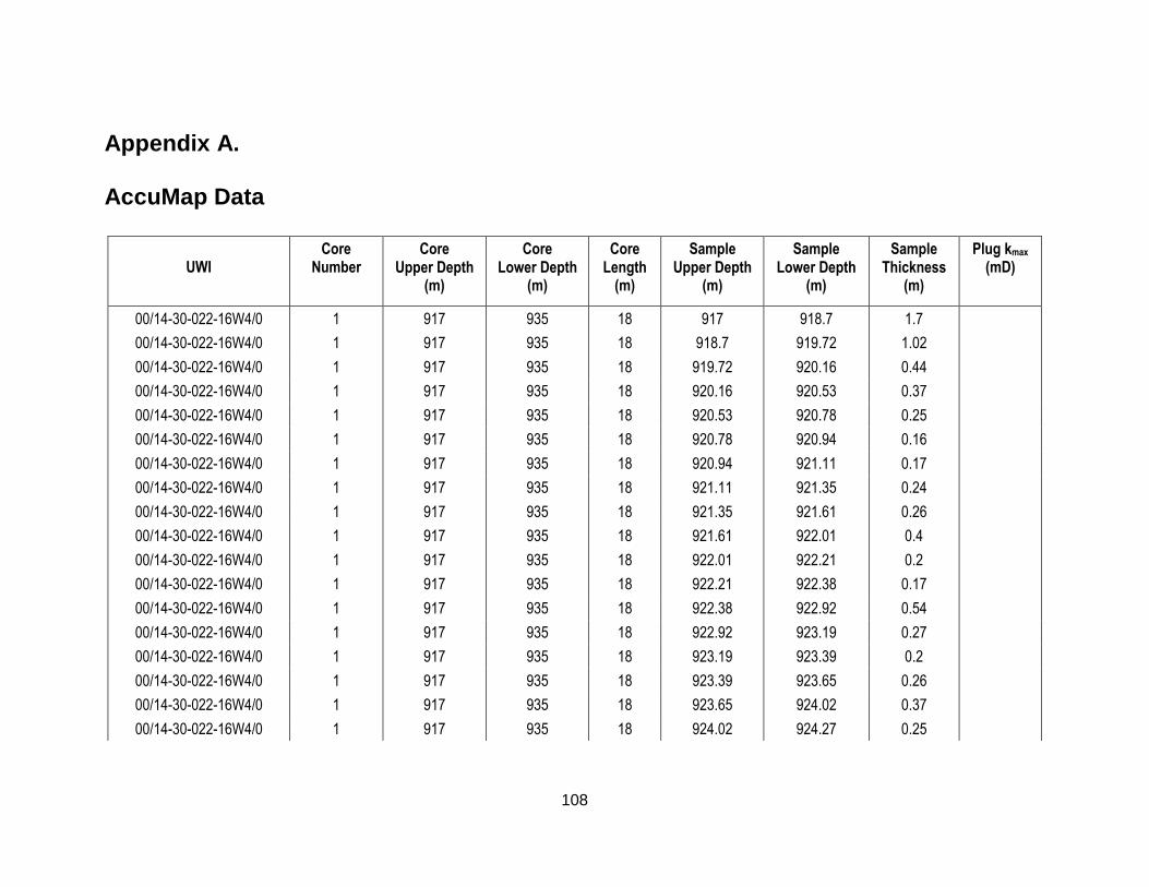
108
Appendix A. AccuMap Data
UWI
Core Number
Core Upper Depth
(m)
Core Lower Depth
(m)
Core Length
(m)
Sample Upper Depth
(m)
Sample Lower Depth
(m)
Sample Thickness
(m)
Plug kmax (mD)
00/14-30-022-16W4/0 1 917 935 18 917 918.7 1.7
00/14-30-022-16W4/0 1 917 935 18 918.7 919.72 1.02
00/14-30-022-16W4/0 1 917 935 18 919.72 920.16 0.44
00/14-30-022-16W4/0 1 917 935 18 920.16 920.53 0.37
00/14-30-022-16W4/0 1 917 935 18 920.53 920.78 0.25
00/14-30-022-16W4/0 1 917 935 18 920.78 920.94 0.16
00/14-30-022-16W4/0 1 917 935 18 920.94 921.11 0.17
00/14-30-022-16W4/0 1 917 935 18 921.11 921.35 0.24
00/14-30-022-16W4/0 1 917 935 18 921.35 921.61 0.26
00/14-30-022-16W4/0 1 917 935 18 921.61 922.01 0.4
00/14-30-022-16W4/0 1 917 935 18 922.01 922.21 0.2
00/14-30-022-16W4/0 1 917 935 18 922.21 922.38 0.17
00/14-30-022-16W4/0 1 917 935 18 922.38 922.92 0.54
00/14-30-022-16W4/0 1 917 935 18 922.92 923.19 0.27
00/14-30-022-16W4/0 1 917 935 18 923.19 923.39 0.2
00/14-30-022-16W4/0 1 917 935 18 923.39 923.65 0.26
00/14-30-022-16W4/0 1 917 935 18 923.65 924.02 0.37
00/14-30-022-16W4/0 1 917 935 18 924.02 924.27 0.25

109
UWI
Core Number
Core Upper Depth
(m)
Core Lower Depth
(m)
Core Length
(m)
Sample Upper Depth
(m)
Sample Lower Depth
(m)
Sample Thickness
(m)
Plug kmax (mD)
00/14-30-022-16W4/0 1 917 935 18 924.27 924.66 0.39
00/14-30-022-16W4/0 1 917 935 18 924.66 925.11 0.45
00/14-30-022-16W4/0 1 917 935 18 925.11 925.57 0.46
00/14-30-022-16W4/0 1 917 935 18 925.57 925.81 0.24
00/14-30-022-16W4/0 1 917 935 18 925.81 925.99 0.18
00/14-30-022-16W4/0 1 917 935 18 925.99 926.19 0.2
00/14-30-022-16W4/0 1 917 935 18 926.19 926.7 0.51
00/14-30-022-16W4/0 1 917 935 18 926.7 926.96 0.26
00/14-30-022-16W4/0 1 917 935 18 926.96 927.22 0.26
00/14-30-022-16W4/0 1 917 935 18 927.22 927.47 0.25
00/14-30-022-16W4/0 1 917 935 18 927.47 927.83 0.36
00/14-30-022-16W4/0 1 917 935 18 927.83 928.23 0.4
00/14-30-022-16W4/0 1 917 935 18 928.23 928.74 0.51
00/14-30-022-16W4/0 1 917 935 18 928.74 929.17 0.43
00/14-30-022-16W4/0 1 917 935 18 929.17 929.63 0.46
00/14-30-022-16W4/0 1 917 935 18 929.63 930.05 0.42
00/14-30-022-16W4/0 1 917 935 18 930.05 930.42 0.37
00/14-30-022-16W4/0 1 917 935 18 930.42 930.82 0.4
00/14-30-022-16W4/0 1 917 935 18 930.82 931.23 0.41
00/14-30-022-16W4/0 1 917 935 18 931.23 931.73 0.5
00/14-30-022-16W4/0 1 917 935 18 931.73 932.05 0.32
00/14-30-022-16W4/0 1 917 935 18 932.05 932.41 0.36
00/14-30-022-16W4/0 1 917 935 18 932.41 932.95 0.54

110
UWI
Core Number
Core Upper Depth
(m)
Core Lower Depth
(m)
Core Length
(m)
Sample Upper Depth
(m)
Sample Lower Depth
(m)
Sample Thickness
(m)
Plug kmax (mD)
00/14-30-022-16W4/0 1 917 935 18 932.95 933.49 0.54
00/14-30-022-16W4/0 1 917 935 18 933.49 934.15 0.66
00/14-30-022-16W4/0 1 917 935 18 934.15 935 0.85
100/04-19-034-08W4/0 1 893.37 903.43 10.06 893.37 896.93 3.56
100/04-19-034-08W4/0 1 893.37 903.43 10.06 896.93 897.03 0.10 32.10
100/04-19-034-08W4/0 1 893.37 903.43 10.06 897.03 897.21 0.18
100/04-19-034-08W4/0 1 893.37 903.43 10.06 897.21 897.39 0.18
100/04-19-034-08W4/0 1 893.37 903.43 10.06 897.39 897.58 0.19
100/04-19-034-08W4/0 1 893.37 903.43 10.06 897.58 897.79 0.21
100/04-19-034-08W4/0 1 893.37 903.43 10.06 897.79 898.03 0.24
100/04-19-034-08W4/0 1 893.37 903.43 10.06 898.03 898.25 0.22
100/04-19-034-08W4/0 1 893.37 903.43 10.06 898.25 898.34 0.09 68.30
100/04-19-034-08W4/0 1 893.37 903.43 10.06 898.34 898.58 0.24 10.60
100/04-19-034-08W4/0 1 893.37 903.43 10.06 898.58 900.53 1.95
100/04-19-034-08W4/0 1 893.37 903.43 10.06 900.53 903.43 2.90
100/04-23-034-08W4/0 1 862.00 871.00 9.00 862.00 869.18 7.18
100/04-23-034-08W4/0 1 862.00 871.00 9.00 869.18 869.45 0.27
100/04-23-034-08W4/0 1 862.00 871.00 9.00 869.45 869.70 0.25
100/04-23-034-08W4/0 1 862.00 871.00 9.00 869.70 870.00 0.30
100/04-23-034-08W4/0 1 862.00 871.00 9.00 870.00 870.33 0.33
100/04-23-034-08W4/0 1 862.00 871.00 9.00 870.33 870.67 0.34
100/04-23-034-08W4/0 1 862.00 871.00 9.00 870.67 871.00 0.33

111
UWI
Core Number
Core Upper Depth
(m)
Core Lower Depth
(m)
Core Length
(m)
Sample Upper Depth
(m)
Sample Lower Depth
(m)
Sample Thickness
(m)
Plug kmax (mD)
100/04-23-034-08W4/0 2 871.00 880.00 9.00 871.00 871.20 0.20
100/04-23-034-08W4/0 2 871.00 880.00 9.00 871.20 871.41 0.21
100/04-23-034-08W4/0 2 871.00 880.00 9.00 871.41 871.47 0.06 31.54
100/04-23-034-08W4/0 2 871.00 880.00 9.00 871.47 871.63 0.16
100/04-23-034-08W4/0 2 871.00 880.00 9.00 871.63 871.66 0.03
100/04-23-034-08W4/0 2 871.00 880.00 9.00 871.66 872.03 0.37
100/04-23-034-08W4/0 2 871.00 880.00 9.00 872.03 872.10 0.07 12.98
100/04-23-034-08W4/0 2 871.00 880.00 9.00 872.10 872.75 0.65
100/04-23-034-08W4/0 2 871.00 880.00 9.00 872.75 873.00 0.25
100/04-23-034-08W4/0 2 871.00 880.00 9.00 873.00 873.27 0.27
100/04-23-034-08W4/0 2 871.00 880.00 9.00 873.27 874.08 0.81
100/04-23-034-08W4/0 2 871.00 880.00 9.00 874.08 874.38 0.30 1.94
100/04-23-034-08W4/0 2 871.00 880.00 9.00 874.38 876.52 2.14
100/04-23-034-08W4/0 2 871.00 880.00 9.00 876.52 876.70 0.18 12.47
100/04-23-034-08W4/0 2 871.00 880.00 9.00 876.70 876.84 0.14
100/04-23-034-08W4/0 2 871.00 880.00 9.00 876.84 877.15 0.31
100/04-23-034-08W4/0 2 871.00 880.00 9.00 877.15 877.42 0.27
100/04-23-034-08W4/0 2 871.00 880.00 9.00 877.42 877.62 0.20 45.79
100/04-23-034-08W4/0 2 871.00 880.00 9.00 877.62 877.85 0.23
100/04-23-034-08W4/0 2 871.00 880.00 9.00 877.85 878.04 0.19 91.03
100/04-23-034-08W4/0 2 871.00 880.00 9.00 878.04 878.32 0.28
100/04-23-034-08W4/0 2 871.00 880.00 9.00 878.32 878.85 0.53
100/04-23-034-08W4/0 2 871.00 880.00 9.00 878.85 879.65 0.80

112
UWI
Core Number
Core Upper Depth
(m)
Core Lower Depth
(m)
Core Length
(m)
Sample Upper Depth
(m)
Sample Lower Depth
(m)
Sample Thickness
(m)
Plug kmax (mD)
100/04-23-034-08W4/0 2 871.00 880.00 9.00 879.65 880.00 0.35
100/04-31-034-08W4/0 1 898.55 900.99 2.44 898.55 899.46 0.91
100/04-31-034-08W4/0 1 898.55 900.99 2.44 899.46 900.07 0.61
100/04-31-034-08W4/0 1 898.55 900.99 2.44 900.07 900.99 0.92
100/04-31-034-08W4/0 2 900.99 908.61 7.62 900.99 904.13 3.14
100/04-31-034-08W4/0 2 900.99 908.61 7.62 904.13 904.25 0.12
100/04-31-034-08W4/0 2 900.99 908.61 7.62 904.25 904.28 0.03
100/04-31-034-08W4/0 2 900.99 908.61 7.62 904.28 904.40 0.12
100/04-31-034-08W4/0 2 900.99 908.61 7.62 904.40 904.43 0.03
100/04-31-034-08W4/0 2 900.99 908.61 7.62 904.43 904.68 0.25
100/04-31-034-08W4/0 2 900.99 908.61 7.62 904.68 904.92 0.24
100/04-31-034-08W4/0 2 900.99 908.61 7.62 904.92 905.13 0.21
100/04-31-034-08W4/0 2 900.99 908.61 7.62 905.13 905.32 0.19
100/04-31-034-08W4/0 2 900.99 908.61 7.62 905.32 905.53 0.21
100/04-31-034-08W4/0 2 900.99 908.61 7.62 905.53 905.84 0.31
100/04-31-034-08W4/0 2 900.99 908.61 7.62 905.84 906.11 0.27
100/04-31-034-08W4/0 2 900.99 908.61 7.62 906.11 906.17 0.06
100/04-31-034-08W4/0 2 900.99 908.61 7.62 906.17 906.32 0.15
100/04-31-034-08W4/0 2 900.99 908.61 7.62 906.32 906.44 0.12
100/04-31-034-08W4/0 2 900.99 908.61 7.62 906.44 906.48 0.04
100/04-31-034-08W4/0 2 900.99 908.61 7.62 906.48 908.00 1.52
100/04-31-034-08W4/0 2 900.99 908.61 7.62 908.00 908.61 0.61

113
UWI
Core Number
Core Upper Depth
(m)
Core Lower Depth
(m)
Core Length
(m)
Sample Upper Depth
(m)
Sample Lower Depth
(m)
Sample Thickness
(m)
Plug kmax (mD)
100/12-05-034-09W4/0 1 882.40 899.16 16.76 882.40 891.39 8.99
100/12-05-034-09W4/0 1 882.40 899.16 16.76 891.39 891.63 0.24 4.40
100/12-05-034-09W4/0 1 882.40 899.16 16.76 891.63 892.03 0.40 0.06
100/12-05-034-09W4/0 1 882.40 899.16 16.76 892.03 892.15 0.12 1.17
100/12-05-034-09W4/0 1 882.40 899.16 16.76 892.15 892.27 0.12 23.30
100/12-05-034-09W4/0 1 882.40 899.16 16.76 892.27 892.52 0.25 22.00
100/12-05-034-09W4/0 1 882.40 899.16 16.76 892.52 896.14 3.62
100/12-05-034-09W4/0 1 882.40 899.16 16.76 896.14 896.42 0.28 2.46
100/12-05-034-09W4/0 1 882.40 899.16 16.76 896.42 896.63 0.21
100/12-05-034-09W4/0 1 882.40 899.16 16.76 896.63 896.75 0.12 1.97
100/12-05-034-09W4/0 1 882.40 899.16 16.76 896.75 899.16 2.41
100/10-16-034-09W4/0 1 883.62 894.59 10.97 883.62 883.86 0.24
100/10-16-034-09W4/0 1 883.62 894.59 10.97 883.86 884.04 0.18
100/10-16-034-09W4/0 1 883.62 894.59 10.97 884.04 890.05 6.01
100/10-16-034-09W4/0 1 883.62 894.59 10.97 890.05 890.20 0.15
100/10-16-034-09W4/0 1 883.62 894.59 10.97 890.20 890.41 0.21 105.00
100/10-16-034-09W4/0 1 883.62 894.59 10.97 890.41 890.50 0.09 134.00
100/10-16-034-09W4/0 1 883.62 894.59 10.97 890.50 890.56 0.06 128.00
100/10-16-034-09W4/0 1 883.62 894.59 10.97 890.56 890.78 0.22
100/10-16-034-09W4/0 1 883.62 894.59 10.97 890.78 890.93 0.15
100/10-16-034-09W4/0 1 883.62 894.59 10.97 890.93 891.14 0.21
100/10-16-034-09W4/0 1 883.62 894.59 10.97 891.14 891.27 0.13
100/10-16-034-09W4/0 1 883.62 894.59 10.97 891.27 891.42 0.15

114
UWI
Core Number
Core Upper Depth
(m)
Core Lower Depth
(m)
Core Length
(m)
Sample Upper Depth
(m)
Sample Lower Depth
(m)
Sample Thickness
(m)
Plug kmax (mD)
100/10-16-034-09W4/0 1 883.62 894.59 10.97 891.42 891.54 0.12
100/10-16-034-09W4/0 1 883.62 894.59 10.97 891.54 891.69 0.15
100/10-16-034-09W4/0 1 883.62 894.59 10.97 891.69 891.78 0.09 104.00
100/10-16-034-09W4/0 1 883.62 894.59 10.97 891.78 891.97 0.19
100/10-16-034-09W4/0 1 883.62 894.59 10.97 891.97 893.16 1.19
100/10-16-034-09W4/0 1 883.62 894.59 10.97 893.16 893.31 0.15
100/10-16-034-09W4/0 1 883.62 894.59 10.97 893.31 893.67 0.36
100/10-16-034-09W4/0 1 883.62 894.59 10.97 893.67 894.59 0.92
100/12-18-034-09W4/0 1 891.54 908.00 16.46 891.54 891.63 0.09 18.50
100/12-18-034-09W4/0 1 891.54 908.00 16.46 891.63 891.78 0.15 45.40
100/12-18-034-09W4/0 1 891.54 908.00 16.46 891.78 893.06 1.28
100/12-18-034-09W4/0 1 891.54 908.00 16.46 893.06 893.31 0.25 0.76
100/12-18-034-09W4/0 1 891.54 908.00 16.46 893.31 895.35 2.04
100/12-18-034-09W4/0 1 891.54 908.00 16.46 895.35 895.56 0.21 0.53
100/12-18-034-09W4/0 1 891.54 908.00 16.46 895.56 895.78 0.22 0.18
100/12-18-034-09W4/0 1 891.54 908.00 16.46 895.78 895.90 0.12 1.76
100/12-18-034-09W4/0 1 891.54 908.00 16.46 895.90 897.36 1.46
100/12-18-034-09W4/0 1 891.54 908.00 16.46 897.36 897.48 0.12 0.47
100/12-18-034-09W4/0 1 891.54 908.00 16.46 897.48 897.67 0.19 42.60
100/12-18-034-09W4/0 1 891.54 908.00 16.46 897.67 897.88 0.21 1052.00
100/12-18-034-09W4/0 1 891.54 908.00 16.46 897.88 898.09 0.21 550.00
100/12-18-034-09W4/0 1 891.54 908.00 16.46 898.09 898.18 0.09 0.58
100/12-18-034-09W4/0 1 891.54 908.00 16.46 898.18 898.40 0.22 407.00

115
UWI
Core Number
Core Upper Depth
(m)
Core Lower Depth
(m)
Core Length
(m)
Sample Upper Depth
(m)
Sample Lower Depth
(m)
Sample Thickness
(m)
Plug kmax (mD)
100/12-18-034-09W4/0 1 891.54 908.00 16.46 898.40 898.61 0.21 395.00
100/12-18-034-09W4/0 1 891.54 908.00 16.46 898.61 898.89 0.28
100/12-18-034-09W4/0 1 891.54 908.00 16.46 898.89 899.13 0.24 258.00
100/12-18-034-09W4/0 1 891.54 908.00 16.46 899.13 899.34 0.21 105.00
100/12-18-034-09W4/0 1 891.54 908.00 16.46 899.34 899.62 0.28 48.50
100/12-18-034-09W4/0 1 891.54 908.00 16.46 899.62 899.89 0.27 12.30
100/12-18-034-09W4/0 1 891.54 908.00 16.46 899.89 904.65 4.76
100/12-18-034-09W4/0 1 891.54 908.00 16.46 904.65 908.00 3.35
100/02-20-034-09W4/0 1 885.44 900.07 14.63 885.44 885.75 0.31 4.84
100/02-20-034-09W4/0 1 885.44 900.07 14.63 885.75 885.90 0.15 3.15
100/02-20-034-09W4/0 1 885.44 900.07 14.63 885.90 886.21 0.31 1.12
100/02-20-034-09W4/0 1 885.44 900.07 14.63 886.21 886.51 0.30 0.92
100/02-20-034-09W4/0 1 885.44 900.07 14.63 886.51 886.82 0.31 0.94
100/02-20-034-09W4/0 1 885.44 900.07 14.63 886.82 887.12 0.30 7.48
100/02-20-034-09W4/0 1 885.44 900.07 14.63 887.12 887.36 0.24 1.35
100/02-20-034-09W4/0 1 885.44 900.07 14.63 887.36 887.61 0.25 35.10
100/02-20-034-09W4/0 1 885.44 900.07 14.63 887.61 887.85 0.24
100/02-20-034-09W4/0 1 885.44 900.07 14.63 887.85 888.16 0.31 0.88
100/02-20-034-09W4/0 1 885.44 900.07 14.63 888.16 888.46 0.30 0.18
100/02-20-034-09W4/0 1 885.44 900.07 14.63 888.46 888.92 0.46
100/02-20-034-09W4/0 1 885.44 900.07 14.63 888.92 889.19 0.27 3.33
100/02-20-034-09W4/0 1 885.44 900.07 14.63 889.19 889.50 0.31 6.16
100/02-20-034-09W4/0 1 885.44 900.07 14.63 889.50 889.68 0.18 87.40

116
UWI
Core Number
Core Upper Depth
(m)
Core Lower Depth
(m)
Core Length
(m)
Sample Upper Depth
(m)
Sample Lower Depth
(m)
Sample Thickness
(m)
Plug kmax (mD)
100/02-20-034-09W4/0 1 885.44 900.07 14.63 889.68 889.99 0.31 0.12
100/02-20-034-09W4/0 1 885.44 900.07 14.63 889.99 890.29 0.30 0.18
100/02-20-034-09W4/0 1 885.44 900.07 14.63 890.29 890.60 0.31 0.47
100/02-20-034-09W4/0 1 885.44 900.07 14.63 890.60 890.87 0.27 0.49
100/02-20-034-09W4/0 1 885.44 900.07 14.63 890.87 891.05 0.18 2.23
100/02-20-034-09W4/0 1 885.44 900.07 14.63 891.05 891.24 0.19 0.82
100/02-20-034-09W4/0 1 885.44 900.07 14.63 891.24 891.54 0.30 7.48
100/02-20-034-09W4/0 1 885.44 900.07 14.63 891.54 891.84 0.30 7.92
100/02-20-034-09W4/0 1 885.44 900.07 14.63 891.84 892.03 0.19 4.84
100/02-20-034-09W4/0 1 885.44 900.07 14.63 892.03 895.59 3.56
100/02-20-034-09W4/0 1 885.44 900.07 14.63 895.59 895.81 0.22 4.05
100/02-20-034-09W4/0 1 885.44 900.07 14.63 895.81 896.02 0.21 467.00
100/02-20-034-09W4/0 1 885.44 900.07 14.63 896.02 896.20 0.18 865.00
100/02-20-034-09W4/0 1 885.44 900.07 14.63 896.20 896.39 0.19
100/02-20-034-09W4/0 1 885.44 900.07 14.63 896.39 896.54 0.15 183.40
100/02-20-034-09W4/0 1 885.44 900.07 14.63 896.54 896.72 0.18 196.00
100/02-20-034-09W4/0 1 885.44 900.07 14.63 896.72 897.03 0.31 0.01
100/02-20-034-09W4/0 1 885.44 900.07 14.63 897.03 897.30 0.27 0.12
100/02-20-034-09W4/0 1 885.44 900.07 14.63 897.30 897.61 0.31 312.00
100/02-20-034-09W4/0 1 885.44 900.07 14.63 897.61 897.91 0.30 145.00
100/02-20-034-09W4/0 1 885.44 900.07 14.63 897.91 900.07 2.16
100/12-20-034-09W4/0 1 888.49 904.34 15.85 888.49 888.55 0.06 88.70
100/12-20-034-09W4/0 1 888.49 904.34 15.85 888.55 888.64 0.09 101.00

117
UWI
Core Number
Core Upper Depth
(m)
Core Lower Depth
(m)
Core Length
(m)
Sample Upper Depth
(m)
Sample Lower Depth
(m)
Sample Thickness
(m)
Plug kmax (mD)
100/12-20-034-09W4/0 1 888.49 904.34 15.85 888.64 888.95 0.31 64.00
100/12-20-034-09W4/0 1 888.49 904.34 15.85 888.95 889.25 0.30 1.52
100/12-20-034-09W4/0 1 888.49 904.34 15.85 889.25 889.56 0.31 67.10
100/12-20-034-09W4/0 1 888.49 904.34 15.85 889.56 889.71 0.15 1.23
100/12-20-034-09W4/0 1 888.49 904.34 15.85 889.71 889.95 0.24 0.88
100/12-20-034-09W4/0 1 888.49 904.34 15.85 889.95 890.11 0.16 41.30
100/12-20-034-09W4/0 1 888.49 904.34 15.85 890.11 890.41 0.30 1.23
100/12-20-034-09W4/0 1 888.49 904.34 15.85 890.41 892.58 2.17
100/12-20-034-09W4/0 1 888.49 904.34 15.85 892.58 892.88 0.30 82.60
100/12-20-034-09W4/0 1 888.49 904.34 15.85 892.88 893.16 0.28
100/12-20-034-09W4/0 1 888.49 904.34 15.85 893.16 893.28 0.12 1.82
100/12-20-034-09W4/0 1 888.49 904.34 15.85 893.28 893.58 0.30
100/12-20-034-09W4/0 1 888.49 904.34 15.85 893.58 893.67 0.09 36.90
100/12-20-034-09W4/0 1 888.49 904.34 15.85 893.67 893.89 0.22 2.69
100/12-20-034-09W4/0 1 888.49 904.34 15.85 893.89 894.71 0.82
100/12-20-034-09W4/0 1 888.49 904.34 15.85 894.71 894.77 0.06 3.81
100/12-20-034-09W4/0 1 888.49 904.34 15.85 894.77 894.86 0.09
100/12-20-034-09W4/0 1 888.49 904.34 15.85 894.86 895.14 0.28 36.90
100/12-20-034-09W4/0 1 888.49 904.34 15.85 895.14 895.26 0.12
100/12-20-034-09W4/0 1 888.49 904.34 15.85 895.26 895.62 0.36 0.35
100/12-20-034-09W4/0 1 888.49 904.34 15.85 895.62 895.69 0.07 1.29
100/12-20-034-09W4/0 1 888.49 904.34 15.85 895.69 895.84 0.15 6.81
100/12-20-034-09W4/0 1 888.49 904.34 15.85 895.84 896.05 0.21

118
UWI
Core Number
Core Upper Depth
(m)
Core Lower Depth
(m)
Core Length
(m)
Sample Upper Depth
(m)
Sample Lower Depth
(m)
Sample Thickness
(m)
Plug kmax (mD)
100/12-20-034-09W4/0 1 888.49 904.34 15.85 896.05 896.26 0.21 1.82
100/12-20-034-09W4/0 1 888.49 904.34 15.85 896.26 901.23 4.97
100/12-20-034-09W4/0 1 888.49 904.34 15.85 901.23 901.48 0.25 161.00
100/12-20-034-09W4/0 1 888.49 904.34 15.85 901.48 901.63 0.15
100/12-20-034-09W4/0 1 888.49 904.34 15.85 901.63 901.72 0.09 168.00
100/12-20-034-09W4/0 1 888.49 904.34 15.85 901.72 901.81 0.09 2.69
100/12-20-034-09W4/0 1 888.49 904.34 15.85 901.81 901.96 0.15 358.00
100/12-20-034-09W4/0 1 888.49 904.34 15.85 901.96 902.12 0.16 857.00
100/12-20-034-09W4/0 1 888.49 904.34 15.85 902.12 902.39 0.27 195.00
100/12-20-034-09W4/0 1 888.49 904.34 15.85 902.39 902.42 0.03
100/12-20-034-09W4/0 1 888.49 904.34 15.85 902.42 902.60 0.18 198.00
100/12-20-034-09W4/0 1 888.49 904.34 15.85 902.60 902.79 0.19 597.00
100/12-20-034-09W4/0 1 888.49 904.34 15.85 902.79 902.88 0.09 1.26
100/12-20-034-09W4/0 1 888.49 904.34 15.85 902.88 903.03 0.15 76.50
100/12-20-034-09W4/0 1 888.49 904.34 15.85 903.03 903.18 0.15 49.50
100/12-20-034-09W4/0 1 888.49 904.34 15.85 903.18 903.40 0.22 74.30
100/12-20-034-09W4/0 1 888.49 904.34 15.85 903.40 903.49 0.09 37.00
100/12-20-034-09W4/0 1 888.49 904.34 15.85 903.49 904.34 0.85
100/04-23-034-09W4/0 1 889.71 898.86 9.15 889.71 890.72 1.01
100/04-23-034-09W4/0 1 889.71 898.86 9.15 890.72 890.81 0.09 21.98
100/04-23-034-09W4/0 1 889.71 898.86 9.15 890.81 890.87 0.06
100/04-23-034-09W4/0 1 889.71 898.86 9.15 890.87 890.99 0.12 0.58
100/04-23-034-09W4/0 1 889.71 898.86 9.15 890.99 891.08 0.09

119
UWI
Core Number
Core Upper Depth
(m)
Core Lower Depth
(m)
Core Length
(m)
Sample Upper Depth
(m)
Sample Lower Depth
(m)
Sample Thickness
(m)
Plug kmax (mD)
100/04-23-034-09W4/0 1 889.71 898.86 9.15 891.08 891.17 0.09 2.51
100/04-23-034-09W4/0 1 889.71 898.86 9.15 891.17 894.80 3.63
100/04-23-034-09W4/0 1 889.71 898.86 9.15 894.80 894.92 0.12 58.80
100/04-23-034-09W4/0 1 889.71 898.86 9.15 894.92 895.08 0.16
100/04-23-034-09W4/0 1 889.71 898.86 9.15 895.08 895.17 0.09
100/04-23-034-09W4/0 1 889.71 898.86 9.15 895.17 895.32 0.15
100/04-23-034-09W4/0 1 889.71 898.86 9.15 895.32 895.47 0.15
100/04-23-034-09W4/0 1 889.71 898.86 9.15 895.47 895.59 0.12
100/04-23-034-09W4/0 1 889.71 898.86 9.15 895.59 895.87 0.28
100/04-23-034-09W4/0 1 889.71 898.86 9.15 895.87 896.05 0.18
100/04-23-034-09W4/0 1 889.71 898.86 9.15 896.05 896.23 0.18
100/04-23-034-09W4/0 1 889.71 898.86 9.15 896.23 896.51 0.28
100/04-23-034-09W4/0 1 889.71 898.86 9.15 896.51 896.72 0.21
100/04-23-034-09W4/0 1 889.71 898.86 9.15 896.72 896.87 0.15
100/04-23-034-09W4/0 1 889.71 898.86 9.15 896.87 897.06 0.19
100/04-23-034-09W4/0 1 889.71 898.86 9.15 897.06 897.18 0.12
100/04-23-034-09W4/0 1 889.71 898.86 9.15 897.18 897.30 0.12
100/04-23-034-09W4/0 1 889.71 898.86 9.15 897.30 897.36 0.06 6.30
100/04-23-034-09W4/0 1 889.71 898.86 9.15 897.36 897.48 0.12
100/04-23-034-09W4/0 1 889.71 898.86 9.15 897.48 897.54 0.06
100/04-23-034-09W4/0 1 889.71 898.86 9.15 897.54 898.49 0.95
100/04-23-034-09W4/0 1 889.71 898.86 9.15 898.49 898.70 0.21
100/04-23-034-09W4/0 1 889.71 898.86 9.15 898.70 898.86 0.16

120
UWI
Core Number
Core Upper Depth
(m)
Core Lower Depth
(m)
Core Length
(m)
Sample Upper Depth
(m)
Sample Lower Depth
(m)
Sample Thickness
(m)
Plug kmax (mD)
100/04-28-034-09W4/0 1 889.41 893.98 4.57 889.41 889.77 0.36
100/04-28-034-09W4/0 1 889.41 893.98 4.57 889.77 890.02 0.25
100/04-28-034-09W4/0 1 889.41 893.98 4.57 890.02 890.11 0.09 18.90
100/04-28-034-09W4/0 1 889.41 893.98 4.57 890.11 890.41 0.30
100/04-28-034-09W4/0 1 889.41 893.98 4.57 890.41 890.69 0.28
100/04-28-034-09W4/0 1 889.41 893.98 4.57 890.69 890.84 0.15
100/04-28-034-09W4/0 1 889.41 893.98 4.57 890.84 891.02 0.18
100/04-28-034-09W4/0 1 889.41 893.98 4.57 891.02 891.14 0.12
100/04-28-034-09W4/0 1 889.41 893.98 4.57 891.14 891.17 0.03
100/04-28-034-09W4/0 1 889.41 893.98 4.57 891.17 891.33 0.16
100/04-28-034-09W4/0 1 889.41 893.98 4.57 891.33 891.51 0.18
100/04-28-034-09W4/0 1 889.41 893.98 4.57 891.51 891.63 0.12
100/04-28-034-09W4/0 1 889.41 893.98 4.57 891.63 891.84 0.21 7.48
100/04-28-034-09W4/0 1 889.41 893.98 4.57 891.84 893.64 1.80
100/04-28-034-09W4/0 1 889.41 893.98 4.57 893.64 893.80 0.16
100/04-28-034-09W4/0 1 889.41 893.98 4.57 893.80 893.98 0.18
100/04-34-034-09W4/0 1 892.45 901.60 9.15 892.45 893.52 1.07
100/04-34-034-09W4/0 1 892.45 901.60 9.15 893.52 893.70 0.18
100/04-34-034-09W4/0 1 892.45 901.60 9.15 893.70 898.61 4.91
100/04-34-034-09W4/0 1 892.45 901.60 9.15 898.61 898.73 0.12
100/04-34-034-09W4/0 1 892.45 901.60 9.15 898.73 898.76 0.03
100/04-34-034-09W4/0 1 892.45 901.60 9.15 898.76 899.01 0.25
100/04-34-034-09W4/0 1 892.45 901.60 9.15 899.01 899.16 0.15

121
UWI
Core Number
Core Upper Depth
(m)
Core Lower Depth
(m)
Core Length
(m)
Sample Upper Depth
(m)
Sample Lower Depth
(m)
Sample Thickness
(m)
Plug kmax (mD)
100/04-34-034-09W4/0 1 892.45 901.60 9.15 899.16 899.31 0.15
100/04-34-034-09W4/0 1 892.45 901.60 9.15 899.31 899.53 0.22
100/04-34-034-09W4/0 1 892.45 901.60 9.15 899.53 899.74 0.21
100/04-34-034-09W4/0 1 892.45 901.60 9.15 899.74 899.95 0.21
100/04-34-034-09W4/0 1 892.45 901.60 9.15 899.95 900.23 0.28
100/04-34-034-09W4/0 1 892.45 901.60 9.15 900.23 900.35 0.12
100/04-34-034-09W4/0 1 892.45 901.60 9.15 900.35 900.99 0.64
100/04-34-034-09W4/0 1 892.45 901.60 9.15 900.99 901.60 0.61
100/12-02-034-10W4/0 1 891.84 903.73 11.89 891.84 891.97 0.13 1.17
100/12-02-034-10W4/0 1 891.84 903.73 11.89 891.97 892.12 0.15 3.69
100/12-02-034-10W4/0 1 891.84 903.73 11.89 892.12 892.24 0.12 0.06
100/12-02-034-10W4/0 1 891.84 903.73 11.89 892.24 892.33 0.09 1.76
100/12-02-034-10W4/0 1 891.84 903.73 11.89 892.33 892.39 0.06 0.35
100/12-02-034-10W4/0 1 891.84 903.73 11.89 892.39 892.55 0.16 41.80
100/12-02-034-10W4/0 1 891.84 903.73 11.89 892.55 892.67 0.12 9.67
100/12-02-034-10W4/0 1 891.84 903.73 11.89 892.67 892.85 0.18 1.34
100/12-02-034-10W4/0 1 891.84 903.73 11.89 892.85 893.03 0.18 1.47
100/12-02-034-10W4/0 1 891.84 903.73 11.89 893.03 893.12 0.09 1.21
100/12-02-034-10W4/0 1 891.84 903.73 11.89 893.12 894.92 1.80
100/12-02-034-10W4/0 1 891.84 903.73 11.89 894.92 895.11 0.19 2.58
100/12-02-034-10W4/0 1 891.84 903.73 11.89 895.11 895.29 0.18 0.82
100/12-02-034-10W4/0 1 891.84 903.73 11.89 895.29 897.21 1.92
100/12-02-034-10W4/0 1 891.84 903.73 11.89 897.21 897.33 0.12 24.60

122
UWI
Core Number
Core Upper Depth
(m)
Core Lower Depth
(m)
Core Length
(m)
Sample Upper Depth
(m)
Sample Lower Depth
(m)
Sample Thickness
(m)
Plug kmax (mD)
100/12-02-034-10W4/0 1 891.84 903.73 11.89 897.33 897.36 0.03
100/12-02-034-10W4/0 1 891.84 903.73 11.89 897.36 897.61 0.25 0.30
100/12-02-034-10W4/0 1 891.84 903.73 11.89 897.61 898.31 0.70
100/12-02-034-10W4/0 1 891.84 903.73 11.89 898.31 898.40 0.09 0.18
100/12-02-034-10W4/0 1 891.84 903.73 11.89 898.40 899.43 1.03
100/12-02-034-10W4/0 1 891.84 903.73 11.89 899.43 899.65 0.22 0.24
100/12-02-034-10W4/0 1 891.84 903.73 11.89 899.65 900.93 1.28
100/12-02-034-10W4/0 1 891.84 903.73 11.89 900.93 901.17 0.24 0.18
100/12-02-034-10W4/0 1 891.84 903.73 11.89 901.17 901.26 0.09 18.50
100/12-02-034-10W4/0 1 891.84 903.73 11.89 901.26 901.35 0.09 5.50
100/12-02-034-10W4/0 1 891.84 903.73 11.89 901.35 901.45 0.10 1.90
100/12-02-034-10W4/0 1 891.84 903.73 11.89 901.45 901.66 0.21 147.00
100/12-02-034-10W4/0 1 891.84 903.73 11.89 901.66 901.75 0.09 105.00
100/12-02-034-10W4/0 1 891.84 903.73 11.89 901.75 901.81 0.06 35.30
100/12-02-034-10W4/0 1 891.84 903.73 11.89 901.81 901.84 0.03 0.01
100/12-02-034-10W4/0 1 891.84 903.73 11.89 901.84 901.87 0.03
100/12-02-034-10W4/0 1 891.84 903.73 11.89 901.87 901.96 0.09 366.00
100/12-02-034-10W4/0 1 891.84 903.73 11.89 901.96 902.06 0.10 0.53
100/12-02-034-10W4/0 1 891.84 903.73 11.89 902.06 902.30 0.24 474.00
100/12-02-034-10W4/0 1 891.84 903.73 11.89 902.30 902.67 0.37
100/12-02-034-10W4/0 1 891.84 903.73 11.89 902.67 903.73 1.06
100/12-09-034-10W4/0 1 883.92 899.46 15.54 883.92 884.22 0.30 1.23
100/12-09-034-10W4/0 1 883.92 899.46 15.54 884.22 884.53 0.31 2.29

123
UWI
Core Number
Core Upper Depth
(m)
Core Lower Depth
(m)
Core Length
(m)
Sample Upper Depth
(m)
Sample Lower Depth
(m)
Sample Thickness
(m)
Plug kmax (mD)
100/12-09-034-10W4/0 1 883.92 899.46 15.54 884.53 884.83 0.30 7.04
100/12-09-034-10W4/0 1 883.92 899.46 15.54 884.83 885.05 0.22 25.10
100/12-09-034-10W4/0 1 883.92 899.46 15.54 885.05 885.29 0.24 5.28
100/12-09-034-10W4/0 1 883.92 899.46 15.54 885.29 885.78 0.49
100/12-09-034-10W4/0 1 883.92 899.46 15.54 885.78 886.08 0.30 0.35
100/12-09-034-10W4/0 1 883.92 899.46 15.54 886.08 886.36 0.28 0.41
100/12-09-034-10W4/0 1 883.92 899.46 15.54 886.36 886.66 0.30 1.41
100/12-09-034-10W4/0 1 883.92 899.46 15.54 886.66 886.97 0.31 1.29
100/12-09-034-10W4/0 1 883.92 899.46 15.54 886.97 887.27 0.30 8.36
100/12-09-034-10W4/0 1 883.92 899.46 15.54 887.27 887.58 0.31 1.41
100/12-09-034-10W4/0 1 883.92 899.46 15.54 887.58 887.88 0.30 1.93
100/12-09-034-10W4/0 1 883.92 899.46 15.54 887.88 889.71 1.83
100/12-09-034-10W4/0 1 883.92 899.46 15.54 889.71 890.02 0.31 1.82
100/12-09-034-10W4/0 1 883.92 899.46 15.54 890.02 890.32 0.30 1.82
100/12-09-034-10W4/0 1 883.92 899.46 15.54 890.32 890.63 0.31 0.70
100/12-09-034-10W4/0 1 883.92 899.46 15.54 890.63 890.81 0.18 0.86
100/12-09-034-10W4/0 1 883.92 899.46 15.54 890.81 894.07 3.26
100/12-09-034-10W4/0 1 883.92 899.46 15.54 894.07 894.25 0.18 5.72
100/12-09-034-10W4/0 1 883.92 899.46 15.54 894.25 894.40 0.15 48.50
100/12-09-034-10W4/0 1 883.92 899.46 15.54 894.40 894.56 0.16 513.00
100/12-09-034-10W4/0 1 883.92 899.46 15.54 894.56 894.71 0.15 1332.00
100/12-09-034-10W4/0 1 883.92 899.46 15.54 894.71 894.92 0.21 490.00
100/12-09-034-10W4/0 1 883.92 899.46 15.54 894.92 895.14 0.22 780.00

124
UWI
Core Number
Core Upper Depth
(m)
Core Lower Depth
(m)
Core Length
(m)
Sample Upper Depth
(m)
Sample Lower Depth
(m)
Sample Thickness
(m)
Plug kmax (mD)
100/12-09-034-10W4/0 1 883.92 899.46 15.54 895.14 895.35 0.21 0.35
100/12-09-034-10W4/0 1 883.92 899.46 15.54 895.35 895.59 0.24 202.00
100/12-09-034-10W4/0 1 883.92 899.46 15.54 895.59 895.75 0.16 188.00
100/12-09-034-10W4/0 1 883.92 899.46 15.54 895.75 895.93 0.18 490.00
100/12-09-034-10W4/0 1 883.92 899.46 15.54 895.93 896.05 0.12 29.80
100/12-09-034-10W4/0 1 883.92 899.46 15.54 896.05 896.29 0.24 0.47
100/12-09-034-10W4/0 1 883.92 899.46 15.54 896.29 899.46 3.17
100/12-12-034-10W4/0 1 886.97 900.38 13.41 886.97 887.70 0.73
100/12-12-034-10W4/0 1 886.97 900.38 13.41 887.70 887.91 0.21 8.79
100/12-12-034-10W4/0 1 886.97 900.38 13.41 887.91 888.00 0.09 1.17
100/12-12-034-10W4/0 1 886.97 900.38 13.41 888.00 888.16 0.16 71.00
100/12-12-034-10W4/0 1 886.97 900.38 13.41 888.16 888.31 0.15 27.40
100/12-12-034-10W4/0 1 886.97 900.38 13.41 888.31 888.46 0.15 10.10
100/12-12-034-10W4/0 1 886.97 900.38 13.41 888.46 890.23 1.77
100/12-12-034-10W4/0 1 886.97 900.38 13.41 890.23 890.53 0.30 53.00
100/12-12-034-10W4/0 1 886.97 900.38 13.41 890.53 890.81 0.28
100/12-12-034-10W4/0 1 886.97 900.38 13.41 890.81 890.96 0.15 13.18
100/12-12-034-10W4/0 1 886.97 900.38 13.41 890.96 896.33 5.37
100/12-12-034-10W4/0 1 886.97 900.38 13.41 896.33 896.60 0.27 3.51
100/12-12-034-10W4/0 1 886.97 900.38 13.41 896.60 896.69 0.09 266.00
100/12-12-034-10W4/0 1 886.97 900.38 13.41 896.69 896.84 0.15 49.50
100/12-12-034-10W4/0 1 886.97 900.38 13.41 896.84 897.03 0.19 450.00
100/12-12-034-10W4/0 1 886.97 900.38 13.41 897.03 897.09 0.06 32.00

125
UWI
Core Number
Core Upper Depth
(m)
Core Lower Depth
(m)
Core Length
(m)
Sample Upper Depth
(m)
Sample Lower Depth
(m)
Sample Thickness
(m)
Plug kmax (mD)
100/12-12-034-10W4/0 1 886.97 900.38 13.41 897.09 897.15 0.06
100/12-12-034-10W4/0 1 886.97 900.38 13.41 897.15 897.36 0.21 170.00
100/12-12-034-10W4/0 1 886.97 900.38 13.41 897.36 897.57 0.21 225.00
100/12-12-034-10W4/0 1 886.97 900.38 13.41 897.57 897.61 0.04
100/12-12-034-10W4/0 1 886.97 900.38 13.41 897.61 897.76 0.15 0.01
100/12-12-034-10W4/0 1 886.97 900.38 13.41 897.76 897.97 0.21 363.00
100/12-12-034-10W4/0 1 886.97 900.38 13.41 897.97 898.09 0.12 207.00
100/12-12-034-10W4/0 1 886.97 900.38 13.41 898.09 898.31 0.22 498.00
100/12-12-034-10W4/0 1 886.97 900.38 13.41 898.31 898.34 0.03
100/12-12-034-10W4/0 1 886.97 900.38 13.41 898.34 898.55 0.21 152.00
100/12-12-034-10W4/0 1 886.97 900.38 13.41 898.55 898.79 0.24 2.93
100/12-12-034-10W4/0 1 886.97 900.38 13.41 898.79 900.38 1.59
100/12-15-034-10W4/0 1 892.15 907.08 14.93 892.15 892.36 0.21 1.52
100/12-15-034-10W4/0 1 892.15 907.08 14.93 892.36 892.58 0.22 2.10
100/12-15-034-10W4/0 1 892.15 907.08 14.93 892.58 892.70 0.12
100/12-15-034-10W4/0 1 892.15 907.08 14.93 892.70 892.82 0.12 1.52
100/12-15-034-10W4/0 1 892.15 907.08 14.93 892.82 892.94 0.12
100/12-15-034-10W4/0 1 892.15 907.08 14.93 892.94 893.19 0.25 1.19
100/12-15-034-10W4/0 1 892.15 907.08 14.93 893.19 893.37 0.18 1.46
100/12-15-034-10W4/0 1 892.15 907.08 14.93 893.37 893.67 0.30 2.10
100/12-15-034-10W4/0 1 892.15 907.08 14.93 893.67 893.89 0.22 2.10
100/12-15-034-10W4/0 1 892.15 907.08 14.93 893.89 894.10 0.21 0.35
100/12-15-034-10W4/0 1 892.15 907.08 14.93 894.10 894.25 0.15 1.70
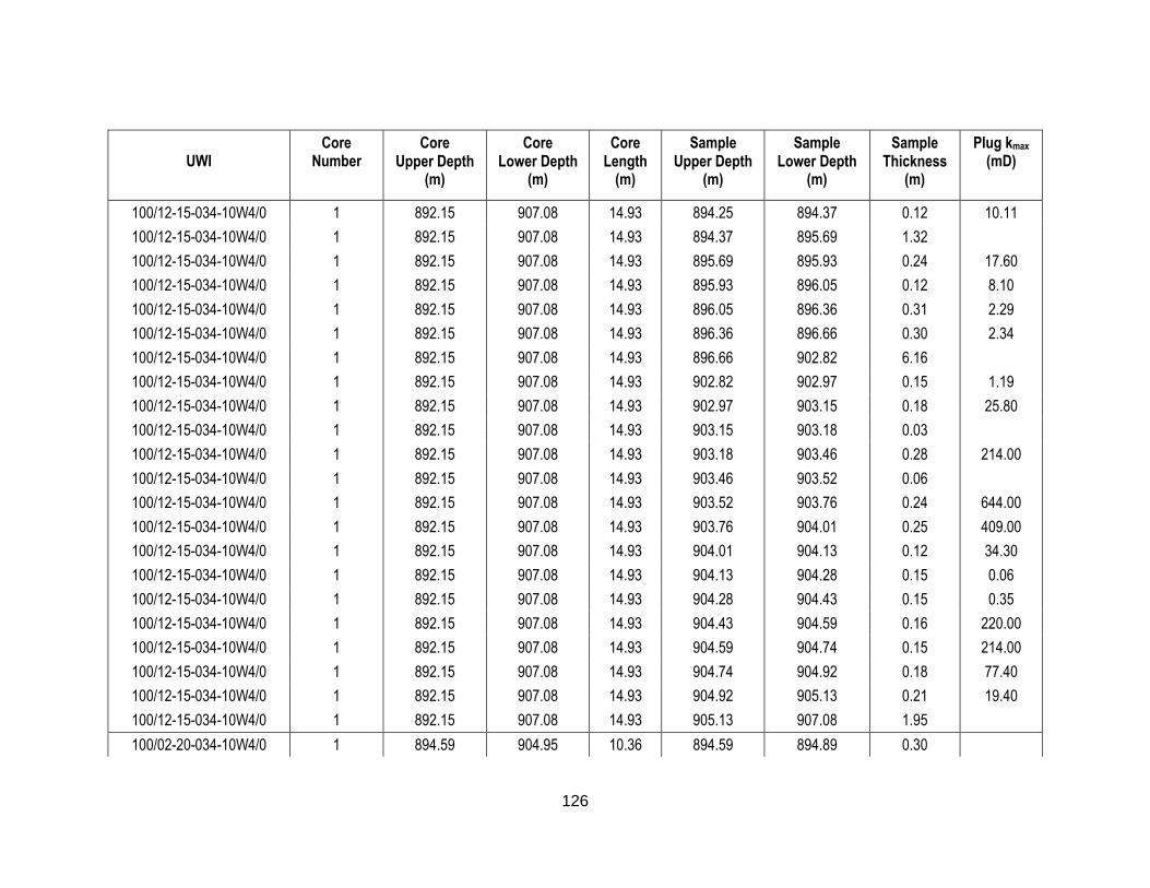
126
UWI
Core Number
Core Upper Depth
(m)
Core Lower Depth
(m)
Core Length
(m)
Sample Upper Depth
(m)
Sample Lower Depth
(m)
Sample Thickness
(m)
Plug kmax (mD)
100/12-15-034-10W4/0 1 892.15 907.08 14.93 894.25 894.37 0.12 10.11
100/12-15-034-10W4/0 1 892.15 907.08 14.93 894.37 895.69 1.32
100/12-15-034-10W4/0 1 892.15 907.08 14.93 895.69 895.93 0.24 17.60
100/12-15-034-10W4/0 1 892.15 907.08 14.93 895.93 896.05 0.12 8.10
100/12-15-034-10W4/0 1 892.15 907.08 14.93 896.05 896.36 0.31 2.29
100/12-15-034-10W4/0 1 892.15 907.08 14.93 896.36 896.66 0.30 2.34
100/12-15-034-10W4/0 1 892.15 907.08 14.93 896.66 902.82 6.16
100/12-15-034-10W4/0 1 892.15 907.08 14.93 902.82 902.97 0.15 1.19
100/12-15-034-10W4/0 1 892.15 907.08 14.93 902.97 903.15 0.18 25.80
100/12-15-034-10W4/0 1 892.15 907.08 14.93 903.15 903.18 0.03
100/12-15-034-10W4/0 1 892.15 907.08 14.93 903.18 903.46 0.28 214.00
100/12-15-034-10W4/0 1 892.15 907.08 14.93 903.46 903.52 0.06
100/12-15-034-10W4/0 1 892.15 907.08 14.93 903.52 903.76 0.24 644.00
100/12-15-034-10W4/0 1 892.15 907.08 14.93 903.76 904.01 0.25 409.00
100/12-15-034-10W4/0 1 892.15 907.08 14.93 904.01 904.13 0.12 34.30
100/12-15-034-10W4/0 1 892.15 907.08 14.93 904.13 904.28 0.15 0.06
100/12-15-034-10W4/0 1 892.15 907.08 14.93 904.28 904.43 0.15 0.35
100/12-15-034-10W4/0 1 892.15 907.08 14.93 904.43 904.59 0.16 220.00
100/12-15-034-10W4/0 1 892.15 907.08 14.93 904.59 904.74 0.15 214.00
100/12-15-034-10W4/0 1 892.15 907.08 14.93 904.74 904.92 0.18 77.40
100/12-15-034-10W4/0 1 892.15 907.08 14.93 904.92 905.13 0.21 19.40
100/12-15-034-10W4/0 1 892.15 907.08 14.93 905.13 907.08 1.95
100/02-20-034-10W4/0 1 894.59 904.95 10.36 894.59 894.89 0.30

127
UWI
Core Number
Core Upper Depth
(m)
Core Lower Depth
(m)
Core Length
(m)
Sample Upper Depth
(m)
Sample Lower Depth
(m)
Sample Thickness
(m)
Plug kmax (mD)
100/02-20-034-10W4/0 1 894.59 904.95 10.36 894.89 895.17 0.28 2.64
100/02-20-034-10W4/0 1 894.59 904.95 10.36 895.17 895.35 0.18 1.76
100/02-20-034-10W4/0 1 894.59 904.95 10.36 895.35 895.59 0.24 2.23
100/02-20-034-10W4/0 1 894.59 904.95 10.36 895.59 895.81 0.22 0.82
100/02-20-034-10W4/0 1 894.59 904.95 10.36 895.81 896.02 0.21 2.23
100/02-20-034-10W4/0 1 894.59 904.95 10.36 896.02 896.11 0.09 17.60
100/02-20-034-10W4/0 1 894.59 904.95 10.36 896.11 896.29 0.18 4.24
100/02-20-034-10W4/0 1 894.59 904.95 10.36 896.29 896.54 0.25 39.50
100/02-20-034-10W4/0 1 894.59 904.95 10.36 896.54 896.72 0.18 21.10
100/02-20-034-10W4/0 1 894.59 904.95 10.36 896.72 896.84 0.12 3.09
100/02-20-034-10W4/0 1 894.59 904.95 10.36 896.84 897.12 0.28 11.00
100/02-20-034-10W4/0 1 894.59 904.95 10.36 897.12 897.36 0.24 13.20
100/02-20-034-10W4/0 1 894.59 904.95 10.36 897.36 897.61 0.25 2.81
100/02-20-034-10W4/0 1 894.59 904.95 10.36 897.61 900.68 3.07
100/02-20-034-10W4/0 1 894.59 904.95 10.36 900.68 900.96 0.28 2.40
100/02-20-034-10W4/0 1 894.59 904.95 10.36 900.96 901.11 0.15 2.17
100/02-20-034-10W4/0 1 894.59 904.95 10.36 901.11 901.23 0.12 33.40
100/02-20-034-10W4/0 1 894.59 904.95 10.36 901.23 901.45 0.22 118.00
100/02-20-034-10W4/0 1 894.59 904.95 10.36 901.45 901.57 0.12 850.00
100/02-20-034-10W4/0 1 894.59 904.95 10.36 901.57 901.78 0.21 253.00
100/02-20-034-10W4/0 1 894.59 904.95 10.36 901.78 901.93 0.15 612.00
100/02-20-034-10W4/0 1 894.59 904.95 10.36 901.93 902.09 0.16
100/02-20-034-10W4/0 1 894.59 904.95 10.36 902.09 902.27 0.18 317.00

128
UWI
Core Number
Core Upper Depth
(m)
Core Lower Depth
(m)
Core Length
(m)
Sample Upper Depth
(m)
Sample Lower Depth
(m)
Sample Thickness
(m)
Plug kmax (mD)
100/02-20-034-10W4/0 1 894.59 904.95 10.36 902.27 902.45 0.18 262.00
100/02-20-034-10W4/0 1 894.59 904.95 10.36 902.45 904.95 2.50
100/02-23-034-10W4/0 1 887.27 904.04 16.77 887.27 887.88 0.61
100/02-23-034-10W4/0 1 887.27 904.04 16.77 887.88 888.16 0.28 2.93
100/02-23-034-10W4/0 1 887.27 904.04 16.77 888.16 888.37 0.21 30.00
100/02-23-034-10W4/0 1 887.27 904.04 16.77 888.37 888.64 0.27 3.03
100/02-23-034-10W4/0 1 887.27 904.04 16.77 888.64 888.86 0.22 0.41
100/02-23-034-10W4/0 1 887.27 904.04 16.77 888.86 889.04 0.18 3.51
100/02-23-034-10W4/0 1 887.27 904.04 16.77 889.04 889.22 0.18 3.03
100/02-23-034-10W4/0 1 887.27 904.04 16.77 889.22 889.47 0.25 67.00
100/02-23-034-10W4/0 1 887.27 904.04 16.77 889.47 889.62 0.15 27.00
100/02-23-034-10W4/0 1 887.27 904.04 16.77 889.62 889.86 0.24 3.75
100/02-23-034-10W4/0 1 887.27 904.04 16.77 889.86 890.11 0.25 7.04
100/02-23-034-10W4/0 1 887.27 904.04 16.77 890.11 890.35 0.24 1.87
100/02-23-034-10W4/0 1 887.27 904.04 16.77 890.35 890.56 0.21 4.80
100/02-23-034-10W4/0 1 887.27 904.04 16.77 890.56 890.72 0.16 53.00
100/02-23-034-10W4/0 1 887.27 904.04 16.77 890.72 891.02 0.30 4.80
100/02-23-034-10W4/0 1 887.27 904.04 16.77 891.02 891.33 0.31 0.94
100/02-23-034-10W4/0 1 887.27 904.04 16.77 891.33 891.63 0.30 4.80
100/02-23-034-10W4/0 1 887.27 904.04 16.77 891.63 891.84 0.21
100/02-23-034-10W4/0 1 887.27 904.04 16.77 891.84 892.09 0.25 2.23
100/02-23-034-10W4/0 1 887.27 904.04 16.77 892.09 892.79 0.70
100/02-23-034-10W4/0 1 887.27 904.04 16.77 892.79 893.09 0.30 9.23

129
UWI
Core Number
Core Upper Depth
(m)
Core Lower Depth
(m)
Core Length
(m)
Sample Upper Depth
(m)
Sample Lower Depth
(m)
Sample Thickness
(m)
Plug kmax (mD)
100/02-23-034-10W4/0 1 887.27 904.04 16.77 893.09 893.22 0.13 64.00
100/02-23-034-10W4/0 1 887.27 904.04 16.77 893.22 893.37 0.15 163.00
100/02-23-034-10W4/0 1 887.27 904.04 16.77 893.37 893.52 0.15 4.05
100/02-23-034-10W4/0 1 887.27 904.04 16.77 893.52 893.77 0.25 3.63
100/02-23-034-10W4/0 1 887.27 904.04 16.77 893.77 894.04 0.27 12.80
100/02-23-034-10W4/0 1 887.27 904.04 16.77 894.04 895.59 1.55
100/02-23-034-10W4/0 1 887.27 904.04 16.77 895.59 895.75 0.16 59.00
100/02-23-034-10W4/0 1 887.27 904.04 16.77 895.75 895.99 0.24 6.15
100/02-23-034-10W4/0 1 887.27 904.04 16.77 895.99 896.29 0.30 4.05
100/02-23-034-10W4/0 1 887.27 904.04 16.77 896.29 896.60 0.31 33.00
100/02-23-034-10W4/0 1 887.27 904.04 16.77 896.60 896.69 0.09
100/02-23-034-10W4/0 1 887.27 904.04 16.77 896.69 896.97 0.28 1.00
100/02-23-034-10W4/0 1 887.27 904.04 16.77 896.97 899.40 2.43
100/02-23-034-10W4/0 1 887.27 904.04 16.77 899.40 899.50 0.10 1.93
100/02-23-034-10W4/0 1 887.27 904.04 16.77 899.50 900.84 1.34
100/02-23-034-10W4/0 1 887.27 904.04 16.77 900.84 900.99 0.15 1.80
100/02-23-034-10W4/0 1 887.27 904.04 16.77 900.99 901.14 0.15 418.00
100/02-23-034-10W4/0 1 887.27 904.04 16.77 901.14 901.29 0.15 308.00
100/02-23-034-10W4/0 1 887.27 904.04 16.77 901.29 901.32 0.03
100/02-23-034-10W4/0 1 887.27 904.04 16.77 901.32 901.57 0.25 658.00
100/02-23-034-10W4/0 1 887.27 904.04 16.77 901.57 901.84 0.27 354.00
100/02-23-034-10W4/0 1 887.27 904.04 16.77 901.84 901.87 0.03
100/02-23-034-10W4/0 1 887.27 904.04 16.77 901.87 902.06 0.19 253.00
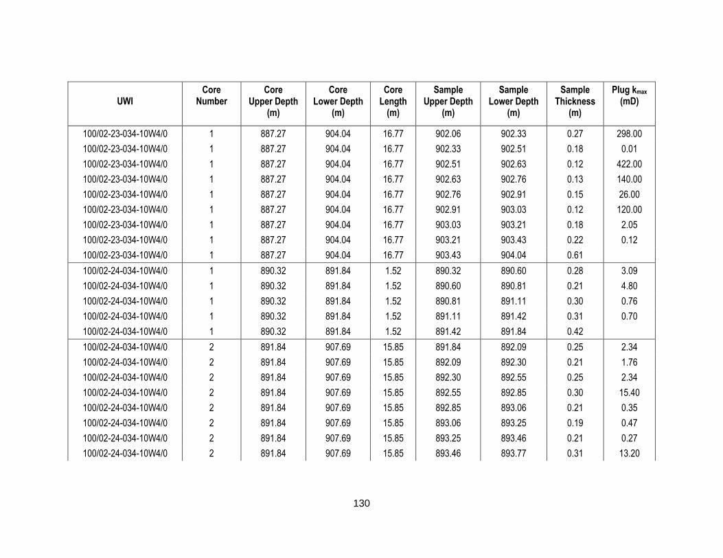
130
UWI
Core Number
Core Upper Depth
(m)
Core Lower Depth
(m)
Core Length
(m)
Sample Upper Depth
(m)
Sample Lower Depth
(m)
Sample Thickness
(m)
Plug kmax (mD)
100/02-23-034-10W4/0 1 887.27 904.04 16.77 902.06 902.33 0.27 298.00
100/02-23-034-10W4/0 1 887.27 904.04 16.77 902.33 902.51 0.18 0.01
100/02-23-034-10W4/0 1 887.27 904.04 16.77 902.51 902.63 0.12 422.00
100/02-23-034-10W4/0 1 887.27 904.04 16.77 902.63 902.76 0.13 140.00
100/02-23-034-10W4/0 1 887.27 904.04 16.77 902.76 902.91 0.15 26.00
100/02-23-034-10W4/0 1 887.27 904.04 16.77 902.91 903.03 0.12 120.00
100/02-23-034-10W4/0 1 887.27 904.04 16.77 903.03 903.21 0.18 2.05
100/02-23-034-10W4/0 1 887.27 904.04 16.77 903.21 903.43 0.22 0.12
100/02-23-034-10W4/0 1 887.27 904.04 16.77 903.43 904.04 0.61
100/02-24-034-10W4/0 1 890.32 891.84 1.52 890.32 890.60 0.28 3.09
100/02-24-034-10W4/0 1 890.32 891.84 1.52 890.60 890.81 0.21 4.80
100/02-24-034-10W4/0 1 890.32 891.84 1.52 890.81 891.11 0.30 0.76
100/02-24-034-10W4/0 1 890.32 891.84 1.52 891.11 891.42 0.31 0.70
100/02-24-034-10W4/0 1 890.32 891.84 1.52 891.42 891.84 0.42
100/02-24-034-10W4/0 2 891.84 907.69 15.85 891.84 892.09 0.25 2.34
100/02-24-034-10W4/0 2 891.84 907.69 15.85 892.09 892.30 0.21 1.76
100/02-24-034-10W4/0 2 891.84 907.69 15.85 892.30 892.55 0.25 2.34
100/02-24-034-10W4/0 2 891.84 907.69 15.85 892.55 892.85 0.30 15.40
100/02-24-034-10W4/0 2 891.84 907.69 15.85 892.85 893.06 0.21 0.35
100/02-24-034-10W4/0 2 891.84 907.69 15.85 893.06 893.25 0.19 0.47
100/02-24-034-10W4/0 2 891.84 907.69 15.85 893.25 893.46 0.21 0.27
100/02-24-034-10W4/0 2 891.84 907.69 15.85 893.46 893.77 0.31 13.20

131
UWI
Core Number
Core Upper Depth
(m)
Core Lower Depth
(m)
Core Length
(m)
Sample Upper Depth
(m)
Sample Lower Depth
(m)
Sample Thickness
(m)
Plug kmax (mD)
100/02-24-034-10W4/0 2 891.84 907.69 15.85 893.77 894.01 0.24 3.33
100/02-24-034-10W4/0 2 891.84 907.69 15.85 894.01 894.22 0.21 20.00
100/02-24-034-10W4/0 2 891.84 907.69 15.85 894.22 894.47 0.25 69.20
100/02-24-034-10W4/0 2 891.84 907.69 15.85 894.47 894.65 0.18 3.27
100/02-24-034-10W4/0 2 891.84 907.69 15.85 894.65 898.21 3.56
100/02-24-034-10W4/0 2 891.84 907.69 15.85 898.21 898.52 0.31 16.30
100/02-24-034-10W4/0 2 891.84 907.69 15.85 898.52 898.82 0.30 120.00
100/02-24-034-10W4/0 2 891.84 907.69 15.85 898.82 899.13 0.31 147.00
100/02-24-034-10W4/0 2 891.84 907.69 15.85 899.13 899.34 0.21 0.12
100/02-24-034-10W4/0 2 891.84 907.69 15.85 899.34 899.56 0.22 230.00
100/02-24-034-10W4/0 2 891.84 907.69 15.85 899.56 899.77 0.21 377.00
100/02-24-034-10W4/0 2 891.84 907.69 15.85 899.77 899.95 0.18 207.00
100/02-24-034-10W4/0 2 891.84 907.69 15.85 899.95 900.14 0.19 16.30
100/02-24-034-10W4/0 2 891.84 907.69 15.85 900.14 907.24 7.10
100/02-24-034-10W4/0 2 891.84 907.69 15.85 907.24 907.69 0.45
100/02-26-034-10W4/0 1 880.87 897.33 16.46 880.87 882.67 1.80
100/02-26-034-10W4/0 1 880.87 897.33 16.46 882.67 882.79 0.12 0.35
100/02-26-034-10W4/0 1 880.87 897.33 16.46 882.79 882.91 0.12 0.01
100/02-26-034-10W4/0 1 880.87 897.33 16.46 882.91 883.04 0.13 0.23
100/02-26-034-10W4/0 1 880.87 897.33 16.46 883.04 883.31 0.27 12.30
100/02-26-034-10W4/0 1 880.87 897.33 16.46 883.31 883.40 0.09
100/02-26-034-10W4/0 1 880.87 897.33 16.46 883.40 883.62 0.22 26.40
100/02-26-034-10W4/0 1 880.87 897.33 16.46 883.62 883.86 0.24 10.10

132
UWI
Core Number
Core Upper Depth
(m)
Core Lower Depth
(m)
Core Length
(m)
Sample Upper Depth
(m)
Sample Lower Depth
(m)
Sample Thickness
(m)
Plug kmax (mD)
100/02-26-034-10W4/0 1 880.87 897.33 16.46 883.86 884.07 0.21 13.20
100/02-26-034-10W4/0 1 880.87 897.33 16.46 884.07 884.32 0.25 7.92
100/02-26-034-10W4/0 1 880.87 897.33 16.46 884.32 884.56 0.24 11.90
100/02-26-034-10W4/0 1 880.87 897.33 16.46 884.56 884.86 0.30 6.16
100/02-26-034-10W4/0 1 880.87 897.33 16.46 884.86 885.14 0.28 4.49
100/02-26-034-10W4/0 1 880.87 897.33 16.46 885.14 885.38 0.24 1.00
100/02-26-034-10W4/0 1 880.87 897.33 16.46 885.38 885.69 0.31 1.06
100/02-26-034-10W4/0 1 880.87 897.33 16.46 885.69 886.60 0.91
100/02-26-034-10W4/0 1 880.87 897.33 16.46 886.60 886.79 0.19 0.88
100/02-26-034-10W4/0 1 880.87 897.33 16.46 886.79 886.91 0.12 20.00
100/02-26-034-10W4/0 1 880.87 897.33 16.46 886.91 887.03 0.12 152.00
100/02-26-034-10W4/0 1 880.87 897.33 16.46 887.03 887.18 0.15 276.00
100/02-26-034-10W4/0 1 880.87 897.33 16.46 887.18 887.36 0.18 26.00
100/02-26-034-10W4/0 1 880.87 897.33 16.46 887.36 887.67 0.31 0.65
100/02-26-034-10W4/0 1 880.87 897.33 16.46 887.67 889.50 1.83
100/02-26-034-10W4/0 1 880.87 897.33 16.46 889.50 889.80 0.30 0.88
100/02-26-034-10W4/0 1 880.87 897.33 16.46 889.80 890.11 0.31 0.59
100/02-26-034-10W4/0 1 880.87 897.33 16.46 890.11 890.41 0.30 6.15
100/02-26-034-10W4/0 1 880.87 897.33 16.46 890.41 890.72 0.31 0.35
100/02-26-034-10W4/0 1 880.87 897.33 16.46 890.72 890.99 0.27 0.59
100/02-26-034-10W4/0 1 880.87 897.33 16.46 890.99 891.30 0.31 2.63
100/02-26-034-10W4/0 1 880.87 897.33 16.46 891.30 894.47 3.17
100/02-26-034-10W4/0 1 880.87 897.33 16.46 894.47 894.65 0.18 376.00

133
UWI
Core Number
Core Upper Depth
(m)
Core Lower Depth
(m)
Core Length
(m)
Sample Upper Depth
(m)
Sample Lower Depth
(m)
Sample Thickness
(m)
Plug kmax (mD)
100/02-26-034-10W4/0 1 880.87 897.33 16.46 894.65 894.86 0.21 312.00
100/02-26-034-10W4/0 1 880.87 897.33 16.46 894.86 895.11 0.25 331.00
100/02-26-034-10W4/0 1 880.87 897.33 16.46 895.11 895.35 0.24 252.00
100/02-26-034-10W4/0 1 880.87 897.33 16.46 895.35 895.59 0.24 262.00
100/02-26-034-10W4/0 1 880.87 897.33 16.46 895.59 895.84 0.25 303.00
100/02-26-034-10W4/0 1 880.87 897.33 16.46 895.84 895.99 0.15 147.00
100/02-26-034-10W4/0 1 880.87 897.33 16.46 895.99 896.11 0.12 3.38
100/02-26-034-10W4/0 1 880.87 897.33 16.46 896.11 896.23 0.12 4.50
100/02-26-034-10W4/0 1 880.87 897.33 16.46 896.23 896.36 0.13 2.97
100/02-26-034-10W4/0 1 880.87 897.33 16.46 896.36 896.48 0.12 0.53
100/02-26-034-10W4/0 1 880.87 897.33 16.46 896.48 897.33 0.85
100/12-26-034-10W4/0 1 879.35 894.59 15.24 879.35 879.38 0.03
100/12-26-034-10W4/0 1 879.35 894.59 15.24 879.38 879.44 0.06 257.00
100/12-26-034-10W4/0 1 879.35 894.59 15.24 879.44 880.99 1.55
100/12-26-034-10W4/0 1 879.35 894.59 15.24 880.99 881.30 0.31 10.10
100/12-26-034-10W4/0 1 879.35 894.59 15.24 881.30 881.60 0.30 9.67
100/12-26-034-10W4/0 1 879.35 894.59 15.24 881.60 881.91 0.31 9.23
100/12-26-034-10W4/0 1 879.35 894.59 15.24 881.91 882.21 0.30 1.40
100/12-26-034-10W4/0 1 879.35 894.59 15.24 882.21 882.52 0.31 0.82
100/12-26-034-10W4/0 1 879.35 894.59 15.24 882.52 882.82 0.30 0.70
100/12-26-034-10W4/0 1 879.35 894.59 15.24 882.82 883.16 0.34
100/12-26-034-10W4/0 1 879.35 894.59 15.24 883.16 883.40 0.24 1.40
100/12-26-034-10W4/0 1 879.35 894.59 15.24 883.40 883.71 0.31 0.35

134
UWI
Core Number
Core Upper Depth
(m)
Core Lower Depth
(m)
Core Length
(m)
Sample Upper Depth
(m)
Sample Lower Depth
(m)
Sample Thickness
(m)
Plug kmax (mD)
100/12-26-034-10W4/0 1 879.35 894.59 15.24 883.71 883.98 0.27 58.00
100/12-26-034-10W4/0 1 879.35 894.59 15.24 883.98 884.10 0.12 47.00
100/12-26-034-10W4/0 1 879.35 894.59 15.24 884.10 884.16 0.06 20.00
100/12-26-034-10W4/0 1 879.35 894.59 15.24 884.16 884.19 0.03
100/12-26-034-10W4/0 1 879.35 894.59 15.24 884.19 884.38 0.19 6.16
100/12-26-034-10W4/0 1 879.35 894.59 15.24 884.38 884.47 0.09 47.00
100/12-26-034-10W4/0 1 879.35 894.59 15.24 884.47 884.77 0.30 2.34
100/12-26-034-10W4/0 1 879.35 894.59 15.24 884.77 885.08 0.31 0.12
100/12-26-034-10W4/0 1 879.35 894.59 15.24 885.08 886.27 1.19
100/12-26-034-10W4/0 1 879.35 894.59 15.24 886.27 886.57 0.30 1.27
100/12-26-034-10W4/0 1 879.35 894.59 15.24 886.57 886.88 0.31 8.79
100/12-26-034-10W4/0 1 879.35 894.59 15.24 886.88 887.18 0.30 0.41
100/12-26-034-10W4/0 1 879.35 894.59 15.24 887.18 887.39 0.21 0.41
100/12-26-034-10W4/0 1 879.35 894.59 15.24 887.39 887.46 0.07 37.00
100/12-26-034-10W4/0 1 879.35 894.59 15.24 887.46 890.81 3.35
100/12-26-034-10W4/0 1 879.35 894.59 15.24 890.81 890.99 0.18 0.12
100/12-26-034-10W4/0 1 879.35 894.59 15.24 890.99 891.11 0.12 19.30
100/12-26-034-10W4/0 1 879.35 894.59 15.24 891.11 891.30 0.19 390.00
100/12-26-034-10W4/0 1 879.35 894.59 15.24 891.30 891.39 0.09
100/12-26-034-10W4/0 1 879.35 894.59 15.24 891.39 891.51 0.12 920.00
100/12-26-034-10W4/0 1 879.35 894.59 15.24 891.51 891.63 0.12 491.00
100/12-26-034-10W4/0 1 879.35 894.59 15.24 891.63 891.75 0.12 644.00
100/12-26-034-10W4/0 1 879.35 894.59 15.24 891.75 891.84 0.09 83.00

135
UWI
Core Number
Core Upper Depth
(m)
Core Lower Depth
(m)
Core Length
(m)
Sample Upper Depth
(m)
Sample Lower Depth
(m)
Sample Thickness
(m)
Plug kmax (mD)
100/12-26-034-10W4/0 1 879.35 894.59 15.24 891.84 892.03 0.19 0.30
100/12-26-034-10W4/0 1 879.35 894.59 15.24 892.03 892.27 0.24 312.00
100/12-26-034-10W4/0 1 879.35 894.59 15.24 892.27 892.39 0.12 156.00
100/12-26-034-10W4/0 1 879.35 894.59 15.24 892.39 892.52 0.13 390.00
100/12-26-034-10W4/0 1 879.35 894.59 15.24 892.52 892.64 0.12 230.00
100/12-26-034-10W4/0 1 879.35 894.59 15.24 892.64 892.85 0.21 1.40
100/12-26-034-10W4/0 1 879.35 894.59 15.24 892.85 893.12 0.27 0.70
100/12-26-034-10W4/0 1 879.35 894.59 15.24 893.12 893.40 0.28 0.41
100/12-26-034-10W4/0 1 879.35 894.59 15.24 893.40 894.59 1.19
100/12-34-034-10W4/0 1 876.30 893.06 16.76 876.30 877.46 1.16
100/12-34-034-10W4/0 1 876.30 893.06 16.76 877.46 877.70 0.24 0.47
100/12-34-034-10W4/0 1 876.30 893.06 16.76 877.70 877.95 0.25 0.48
100/12-34-034-10W4/0 1 876.30 893.06 16.76 877.95 878.25 0.30 5.28
100/12-34-034-10W4/0 1 876.30 893.06 16.76 878.25 878.49 0.24 0.94
100/12-34-034-10W4/0 1 876.30 893.06 16.76 878.49 878.80 0.31 1.06
100/12-34-034-10W4/0 1 876.30 893.06 16.76 878.80 879.10 0.30 2.40
100/12-34-034-10W4/0 1 876.30 893.06 16.76 879.10 879.35 0.25 0.53
100/12-34-034-10W4/0 1 876.30 893.06 16.76 879.35 879.50 0.15 6.60
100/12-34-034-10W4/0 1 876.30 893.06 16.76 879.50 884.41 4.91
100/12-34-034-10W4/0 1 876.30 893.06 16.76 884.41 884.68 0.27 408.00
100/12-34-034-10W4/0 1 876.30 893.06 16.76 884.68 884.80 0.12 475.00
100/12-34-034-10W4/0 1 876.30 893.06 16.76 884.80 884.90 0.10
100/12-34-034-10W4/0 1 876.30 893.06 16.76 884.90 885.08 0.18 704.00

136
UWI
Core Number
Core Upper Depth
(m)
Core Lower Depth
(m)
Core Length
(m)
Sample Upper Depth
(m)
Sample Lower Depth
(m)
Sample Thickness
(m)
Plug kmax (mD)
100/12-34-034-10W4/0 1 876.30 893.06 16.76 885.08 885.32 0.24 22.30
100/12-34-034-10W4/0 1 876.30 893.06 16.76 885.32 885.54 0.22 0.01
100/12-34-034-10W4/0 1 876.30 893.06 16.76 885.54 885.72 0.18 368.00
100/12-34-034-10W4/0 1 876.30 893.06 16.76 885.72 885.96 0.24 118.00
100/12-34-034-10W4/0 1 876.30 893.06 16.76 885.96 886.11 0.15 13.20
100/12-34-034-10W4/0 1 876.30 893.06 16.76 886.11 886.24 0.13 2.40
100/12-34-034-10W4/0 1 876.30 893.06 16.76 886.24 891.54 5.30
100/12-34-034-10W4/0 1 876.30 893.06 16.76 891.54 893.06 1.52
100/02-36-034-10W4/0 1 882.40 897.64 15.24 882.40 891.33 8.93
100/02-36-034-10W4/0 1 882.40 897.64 15.24 891.33 891.57 0.24 5.75
100/02-36-034-10W4/0 1 882.40 897.64 15.24 891.57 891.88 0.31 5.26
100/02-36-034-10W4/0 1 882.40 897.64 15.24 891.88 892.06 0.18 6.15
100/02-36-034-10W4/0 1 882.40 897.64 15.24 892.06 892.21 0.15 47.50
100/02-36-034-10W4/0 1 882.40 897.64 15.24 892.21 892.52 0.31 0.87
100/02-36-034-10W4/0 1 882.40 897.64 15.24 892.52 893.31 0.79
100/02-36-034-10W4/0 1 882.40 897.64 15.24 893.31 893.61 0.30 0.70
100/02-36-034-10W4/0 1 882.40 897.64 15.24 893.61 893.98 0.37
100/02-36-034-10W4/0 1 882.40 897.64 15.24 893.98 894.10 0.12 1.92
100/02-36-034-10W4/0 1 882.40 897.64 15.24 894.10 894.22 0.12 0.01
100/02-36-034-10W4/0 1 882.40 897.64 15.24 894.22 894.53 0.31 1.50
100/02-36-034-10W4/0 1 882.40 897.64 15.24 894.53 894.68 0.15
100/02-36-034-10W4/0 1 882.40 897.64 15.24 894.68 894.86 0.18 0.82
100/02-36-034-10W4/0 1 882.40 897.64 15.24 894.86 895.05 0.19 0.53

137
UWI
Core Number
Core Upper Depth
(m)
Core Lower Depth
(m)
Core Length
(m)
Sample Upper Depth
(m)
Sample Lower Depth
(m)
Sample Thickness
(m)
Plug kmax (mD)
100/02-36-034-10W4/0 1 882.40 897.64 15.24 895.05 896.57 1.52
100/02-36-034-10W4/0 1 882.40 897.64 15.24 896.57 897.64 1.07
100/10-01-035-09W4/0 1 897.94 910.44 12.50 897.94 898.15 0.21 2.87
100/10-01-035-09W4/0 1 897.94 910.44 12.50 898.15 898.21 0.06 33.00
100/10-01-035-09W4/0 1 897.94 910.44 12.50 898.21 898.34 0.13 31.70
100/10-01-035-09W4/0 1 897.94 910.44 12.50 898.34 898.43 0.09 26.40
100/10-01-035-09W4/0 1 897.94 910.44 12.50 898.43 898.55 0.12 36.50
100/10-01-035-09W4/0 1 897.94 910.44 12.50 898.55 898.64 0.09 118.00
100/10-01-035-09W4/0 1 897.94 910.44 12.50 898.64 898.73 0.09 6.15
100/10-01-035-09W4/0 1 897.94 910.44 12.50 898.73 898.89 0.16 21.10
100/10-01-035-09W4/0 1 897.94 910.44 12.50 898.89 899.13 0.24 1.35
100/10-01-035-09W4/0 1 897.94 910.44 12.50 899.13 900.10 0.97
100/10-01-035-09W4/0 1 897.94 910.44 12.50 900.10 900.23 0.13 16.80
100/10-01-035-09W4/0 1 897.94 910.44 12.50 900.23 900.50 0.27 1.64
100/10-01-035-09W4/0 1 897.94 910.44 12.50 900.50 900.74 0.24 1.35
100/10-01-035-09W4/0 1 897.94 910.44 12.50 900.74 900.99 0.25 4.11
100/10-01-035-09W4/0 1 897.94 910.44 12.50 900.99 902.51 1.52
100/10-01-035-09W4/0 1 897.94 910.44 12.50 902.51 902.54 0.03 3.21
100/10-01-035-09W4/0 1 897.94 910.44 12.50 902.54 902.60 0.06
100/10-01-035-09W4/0 1 897.94 910.44 12.50 902.60 902.70 0.10 3.21
100/10-01-035-09W4/0 1 897.94 910.44 12.50 902.70 902.79 0.09
100/10-01-035-09W4/0 1 897.94 910.44 12.50 902.79 902.82 0.03 3.21
100/10-01-035-09W4/0 1 897.94 910.44 12.50 902.82 903.15 0.33

138
UWI
Core Number
Core Upper Depth
(m)
Core Lower Depth
(m)
Core Length
(m)
Sample Upper Depth
(m)
Sample Lower Depth
(m)
Sample Thickness
(m)
Plug kmax (mD)
100/10-01-035-09W4/0 1 897.94 910.44 12.50 903.15 903.27 0.12 0.65
100/10-01-035-09W4/0 1 897.94 910.44 12.50 903.27 904.68 1.41
100/10-01-035-09W4/0 1 897.94 910.44 12.50 904.68 904.77 0.09 13.20
100/10-01-035-09W4/0 1 897.94 910.44 12.50 904.77 906.11 1.34
100/10-01-035-09W4/0 1 897.94 910.44 12.50 906.11 906.35 0.24 30.80
100/10-01-035-09W4/0 1 897.94 910.44 12.50 906.35 906.54 0.19 1340.00
100/10-01-035-09W4/0 1 897.94 910.44 12.50 906.54 906.75 0.21 950.00
100/10-01-035-09W4/0 1 897.94 910.44 12.50 906.75 906.93 0.18 711.00
100/10-01-035-09W4/0 1 897.94 910.44 12.50 906.93 907.02 0.09 619.00
100/10-01-035-09W4/0 1 897.94 910.44 12.50 907.02 907.15 0.13 216.00
100/10-01-035-09W4/0 1 897.94 910.44 12.50 907.15 907.33 0.18 0.01
100/10-01-035-09W4/0 1 897.94 910.44 12.50 907.33 907.48 0.15 140.00
100/10-01-035-09W4/0 1 897.94 910.44 12.50 907.48 907.63 0.15 123.00
100/10-01-035-09W4/0 1 897.94 910.44 12.50 907.63 907.79 0.16 102.00
100/10-01-035-09W4/0 1 897.94 910.44 12.50 907.79 908.00 0.21 111.00
100/10-01-035-09W4/0 1 897.94 910.44 12.50 908.00 908.21 0.21
100/10-01-035-09W4/0 1 897.94 910.44 12.50 908.21 908.27 0.06 5.28
100/10-01-035-09W4/0 1 897.94 910.44 12.50 908.27 908.91 0.64
100/10-01-035-09W4/0 1 897.94 910.44 12.50 908.91 910.44 1.53
100/06-16-035-09W4/0 1 888.80 902.82 14.02 888.80 893.06 4.26
100/06-16-035-09W4/0 1 888.80 902.82 14.02 893.06 893.16 0.10 0.88
100/06-16-035-09W4/0 1 888.80 902.82 14.02 893.16 893.31 0.15 11.00
100/06-16-035-09W4/0 1 888.80 902.82 14.02 893.31 893.49 0.18 19.30
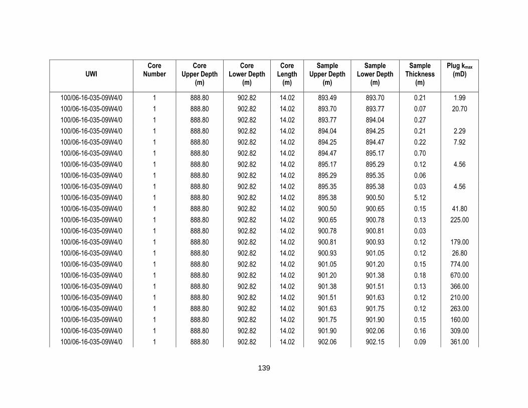
139
UWI
Core Number
Core Upper Depth
(m)
Core Lower Depth
(m)
Core Length
(m)
Sample Upper Depth
(m)
Sample Lower Depth
(m)
Sample Thickness
(m)
Plug kmax (mD)
100/06-16-035-09W4/0 1 888.80 902.82 14.02 893.49 893.70 0.21 1.99
100/06-16-035-09W4/0 1 888.80 902.82 14.02 893.70 893.77 0.07 20.70
100/06-16-035-09W4/0 1 888.80 902.82 14.02 893.77 894.04 0.27
100/06-16-035-09W4/0 1 888.80 902.82 14.02 894.04 894.25 0.21 2.29
100/06-16-035-09W4/0 1 888.80 902.82 14.02 894.25 894.47 0.22 7.92
100/06-16-035-09W4/0 1 888.80 902.82 14.02 894.47 895.17 0.70
100/06-16-035-09W4/0 1 888.80 902.82 14.02 895.17 895.29 0.12 4.56
100/06-16-035-09W4/0 1 888.80 902.82 14.02 895.29 895.35 0.06
100/06-16-035-09W4/0 1 888.80 902.82 14.02 895.35 895.38 0.03 4.56
100/06-16-035-09W4/0 1 888.80 902.82 14.02 895.38 900.50 5.12
100/06-16-035-09W4/0 1 888.80 902.82 14.02 900.50 900.65 0.15 41.80
100/06-16-035-09W4/0 1 888.80 902.82 14.02 900.65 900.78 0.13 225.00
100/06-16-035-09W4/0 1 888.80 902.82 14.02 900.78 900.81 0.03
100/06-16-035-09W4/0 1 888.80 902.82 14.02 900.81 900.93 0.12 179.00
100/06-16-035-09W4/0 1 888.80 902.82 14.02 900.93 901.05 0.12 26.80
100/06-16-035-09W4/0 1 888.80 902.82 14.02 901.05 901.20 0.15 774.00
100/06-16-035-09W4/0 1 888.80 902.82 14.02 901.20 901.38 0.18 670.00
100/06-16-035-09W4/0 1 888.80 902.82 14.02 901.38 901.51 0.13 366.00
100/06-16-035-09W4/0 1 888.80 902.82 14.02 901.51 901.63 0.12 210.00
100/06-16-035-09W4/0 1 888.80 902.82 14.02 901.63 901.75 0.12 263.00
100/06-16-035-09W4/0 1 888.80 902.82 14.02 901.75 901.90 0.15 160.00
100/06-16-035-09W4/0 1 888.80 902.82 14.02 901.90 902.06 0.16 309.00
100/06-16-035-09W4/0 1 888.80 902.82 14.02 902.06 902.15 0.09 361.00

140
UWI
Core Number
Core Upper Depth
(m)
Core Lower Depth
(m)
Core Length
(m)
Sample Upper Depth
(m)
Sample Lower Depth
(m)
Sample Thickness
(m)
Plug kmax (mD)
100/06-16-035-09W4/0 1 888.80 902.82 14.02 902.15 902.33 0.18 516.00
100/06-16-035-09W4/0 1 888.80 902.82 14.02 902.33 902.45 0.12 10.10
100/06-16-035-09W4/0 1 888.80 902.82 14.02 902.45 902.60 0.15 163.00
100/06-16-035-09W4/0 1 888.80 902.82 14.02 902.60 902.76 0.16 194.00
100/06-16-035-09W4/0 1 888.80 902.82 14.02 902.76 902.82 0.06
100/02-26-035-09W4/0 1 895.70 905.00 9.30 895.70 903.97 8.27
100/02-26-035-09W4/0 1 895.70 905.00 9.30 903.97 904.12 0.15 3.13
100/02-26-035-09W4/0 1 895.70 905.00 9.30 904.12 904.39 0.27
100/02-26-035-09W4/0 1 895.70 905.00 9.30 904.39 904.61 0.22
100/02-26-035-09W4/0 1 895.70 905.00 9.30 904.61 904.72 0.11 1.38
100/02-26-035-09W4/0 1 895.70 905.00 9.30 904.72 905.00 0.28
100/02-26-035-09W4/0 2 905.00 912.50 7.50 905.00 908.53 3.53
100/02-26-035-09W4/0 2 905.00 912.50 7.50 908.53 908.69 0.16 2.85
100/02-26-035-09W4/0 2 905.00 912.50 7.50 908.69 908.89 0.20 2.30
100/02-26-035-09W4/0 2 905.00 912.50 7.50 908.89 909.11 0.22
100/02-26-035-09W4/0 2 905.00 912.50 7.50 909.11 909.20 0.09 1.34
100/02-26-035-09W4/0 2 905.00 912.50 7.50 909.20 909.42 0.22
100/02-26-035-09W4/0 2 905.00 912.50 7.50 909.42 909.61 0.19 1.29
100/02-26-035-09W4/0 2 905.00 912.50 7.50 909.61 909.83 0.22 1.92
100/02-26-035-09W4/0 2 905.00 912.50 7.50 909.83 909.93 0.10 1.30
100/02-26-035-09W4/0 2 905.00 912.50 7.50 909.93 910.13 0.20 2.20
100/02-26-035-09W4/0 2 905.00 912.50 7.50 910.13 910.36 0.23 0.45

141
UWI
Core Number
Core Upper Depth
(m)
Core Lower Depth
(m)
Core Length
(m)
Sample Upper Depth
(m)
Sample Lower Depth
(m)
Sample Thickness
(m)
Plug kmax (mD)
100/02-26-035-09W4/0 2 905.00 912.50 7.50 910.36 910.69 0.33
100/02-26-035-09W4/0 2 905.00 912.50 7.50 910.69 910.93 0.24 1.42
100/02-26-035-09W4/0 2 905.00 912.50 7.50 910.93 911.02 0.09 157.00
100/02-26-035-09W4/0 2 905.00 912.50 7.50 911.02 911.07 0.05 105.00
100/02-26-035-09W4/0 2 905.00 912.50 7.50 911.07 911.20 0.13
100/02-26-035-09W4/0 2 905.00 912.50 7.50 911.20 911.29 0.09 114.00
100/02-26-035-09W4/0 2 905.00 912.50 7.50 911.29 911.59 0.30 174.00
100/02-26-035-09W4/0 2 905.00 912.50 7.50 911.59 911.78 0.19 109.00
100/02-26-035-09W4/0 2 905.00 912.50 7.50 911.78 911.86 0.08 83.50
100/02-26-035-09W4/0 2 905.00 912.50 7.50 911.86 911.96 0.10 2.64
100/02-26-035-09W4/0 2 905.00 912.50 7.50 911.96 912.13 0.17 1.77
100/02-26-035-09W4/0 2 905.00 912.50 7.50 912.13 912.50 0.37
100/15-02-035-10W4/0 1 884.83 890.93 6.10 885.75 885.93 0.18
100/15-02-035-10W4/0 1 884.83 890.93 6.10 885.93 886.05 0.12
100/15-02-035-10W4/0 1 884.83 890.93 6.10 886.05 886.14 0.09 135.00
100/15-02-035-10W4/0 1 884.83 890.93 6.10 886.14 886.45 0.31
100/15-02-035-10W4/0 1 884.83 890.93 6.10 886.45 886.63 0.18
100/15-02-035-10W4/0 1 884.83 890.93 6.10 886.63 886.75 0.12
100/15-02-035-10W4/0 1 884.83 890.93 6.10 886.75 886.88 0.13
100/15-02-035-10W4/0 1 884.83 890.93 6.10 886.88 887.03 0.15
100/15-02-035-10W4/0 1 884.83 890.93 6.10 887.03 887.21 0.18
100/15-02-035-10W4/0 1 884.83 890.93 6.10 887.21 887.39 0.18
100/15-02-035-10W4/0 1 884.83 890.93 6.10 887.39 887.61 0.22 3.40

142
UWI
Core Number
Core Upper Depth
(m)
Core Lower Depth
(m)
Core Length
(m)
Sample Upper Depth
(m)
Sample Lower Depth
(m)
Sample Thickness
(m)
Plug kmax (mD)
100/15-02-035-10W4/0 1 884.83 890.93 6.10 887.61 887.73 0.12 42.30
100/15-02-035-10W4/0 1 884.83 890.93 6.10 887.73 890.93 3.20
100/13-15-035-10W4/0 1 877.82 887.58 9.76 877.82 881.51 3.69
100/13-15-035-10W4/0 1 877.82 887.58 9.76 881.51 881.66 0.15 1.23
100/13-15-035-10W4/0 1 877.82 887.58 9.76 881.66 881.79 0.13
100/13-15-035-10W4/0 1 877.82 887.58 9.76 881.79 881.82 0.03 1.17
100/13-15-035-10W4/0 1 877.82 887.58 9.76 881.82 882.06 0.24
100/13-15-035-10W4/0 1 877.82 887.58 9.76 882.06 882.21 0.15 20.22
100/13-15-035-10W4/0 1 877.82 887.58 9.76 882.21 882.37 0.16 3.99
100/13-15-035-10W4/0 1 877.82 887.58 9.76 882.37 882.52 0.15 1.87
100/13-15-035-10W4/0 1 877.82 887.58 9.76 882.52 882.70 0.18 1.47
100/13-15-035-10W4/0 1 877.82 887.58 9.76 882.70 882.85 0.15 3.33
100/13-15-035-10W4/0 1 877.82 887.58 9.76 882.85 882.94 0.09 2.11
100/13-15-035-10W4/0 1 877.82 887.58 9.76 882.94 883.10 0.16 60.90
100/13-15-035-10W4/0 1 877.82 887.58 9.76 883.10 884.74 1.64
100/13-15-035-10W4/0 1 877.82 887.58 9.76 884.74 884.86 0.12 22.87
100/13-15-035-10W4/0 1 877.82 887.58 9.76 884.86 885.02 0.16 449.00
100/13-15-035-10W4/0 1 877.82 887.58 9.76 885.02 885.17 0.15 13.19
100/13-15-035-10W4/0 1 877.82 887.58 9.76 885.17 885.47 0.30 0.18
100/13-15-035-10W4/0 1 877.82 887.58 9.76 885.47 885.60 0.13 17.15
100/13-15-035-10W4/0 1 877.82 887.58 9.76 885.60 885.72 0.12 309.00
100/13-15-035-10W4/0 1 877.82 887.58 9.76 885.72 885.87 0.15 320.00
100/13-15-035-10W4/0 1 877.82 887.58 9.76 885.87 886.02 0.15 291.00

143
UWI
Core Number
Core Upper Depth
(m)
Core Lower Depth
(m)
Core Length
(m)
Sample Upper Depth
(m)
Sample Lower Depth
(m)
Sample Thickness
(m)
Plug kmax (mD)
100/13-15-035-10W4/0 1 877.82 887.58 9.76 886.02 886.24 0.22 54.70
100/13-15-035-10W4/0 1 877.82 887.58 9.76 886.24 887.58 1.34
100/07-31-035-10W4/0 1 892.00 901.00 9.00 892.00 894.64 2.64
100/07-31-035-10W4/0 1 892.00 901.00 9.00 894.64 894.75 0.11 1.76
100/07-31-035-10W4/0 1 892.00 901.00 9.00 894.75 894.91 0.16 198.00
100/07-31-035-10W4/0 1 892.00 901.00 9.00 894.91 895.06 0.15 15.80
100/07-31-035-10W4/0 1 892.00 901.00 9.00 895.06 895.39 0.33 0.25
100/07-31-035-10W4/0 1 892.00 901.00 9.00 895.39 895.56 0.17 0.63
100/07-31-035-10W4/0 1 892.00 901.00 9.00 895.56 895.71 0.15 11.00
100/07-31-035-10W4/0 1 892.00 901.00 9.00 895.71 895.88 0.17 177.00
100/07-31-035-10W4/0 1 892.00 901.00 9.00 895.88 895.96 0.08
100/07-31-035-10W4/0 1 892.00 901.00 9.00 895.96 896.03 0.07 25.30
100/07-31-035-10W4/0 1 892.00 901.00 9.00 896.03 896.16 0.13 42.80
100/07-31-035-10W4/0 1 892.00 901.00 9.00 896.16 896.34 0.18 5.31
100/07-31-035-10W4/0 1 892.00 901.00 9.00 896.34 896.45 0.11 91.70
100/07-31-035-10W4/0 1 892.00 901.00 9.00 896.45 897.81 1.36 1.46
100/07-31-035-10W4/0 1 892.00 901.00 9.00 897.81 899.00 1.19 1.29
100/07-31-035-10W4/0 1 892.00 901.00 9.00 899.00 901.00 2.00
100/07-31-035-10W4/0 2 901.00 910.00 9.00 901.00 910.00 9.00

144
Appendix B. Core Log Data and Geophysical Well Logs
The attached CD-ROM contains image files of the core logs for the 28 studied core intervals, as well as the 13 geophysical well logs used in the construction of cross sections.

145
Appendix C. Horizontal Equivalent K
Well ID Sample
# dh
(m)a
A (m2)a
dl (m)a
Bed/bedset Composite
% Q Discrepancy
Average Q (x100m3/s)
Average Q (m3/s) Kxy (m/s)
Average Q (x100m3/s)
Average Q (m3/s) Kxy (m/s)
12-20-034-09W4 1 1 268 10 2.84E-04 2.84E-06 1.06E-07 2.86E-04 2.86E-06 1.07E-07 1%
2b 1 18 10 2.49E-09 2.49E-11 1.38E-11 9.26E-07 9.26E-09 5.14E-09 37116%
3 1 272 10 3.34E-04 3.34E-06 1.23E-07 3.36E-04 3.36E-06 1.23E-07 1%
4 1 232 10 4.66E-04 4.66E-06 2.01E-07 4.65E-04 4.65E-06 2.01E-07 0%
5 1 142 10 2.81E-06 2.81E-08 1.98E-09 2.92E-06 2.92E-08 2.06E-09 4%
6 1 214 10 7.79E-05 7.79E-07 3.64E-08 7.71E-05 7.71E-07 3.60E-08 -1%
7 1 66 10 1.80E-04 1.80E-06 2.73E-07 1.81E-04 1.81E-06 2.74E-07 0%
8 1 3 10 6.69E-07 6.69E-09 2.23E-08 6.94E-07 6.94E-09 2.31E-08 4%
9 1 185 10 1.77E-03 1.77E-05 9.59E-07 1.77E-03 1.77E-05 9.59E-07 0%
10 1 47 10 4.19E-06 4.19E-08 8.92E-09 4.17E-06 4.17E-08 8.87E-09 -1%
04-28-034-09W4 1 1 32 10 4.43E-05 4.43E-07 1.38E-07 4.43E-05 4.43E-07 1.39E-07 0%
2 1 141 10 1.76E-03 1.76E-05 1.25E-06 1.76E-03 1.76E-05 1.25E-06 0%
3 1 105 10 2.41E-04 2.41E-06 2.30E-07 2.42E-04 2.42E-06 2.30E-07 0%
4 1 60 10 3.15E-06 3.15E-08 5.26E-09 3.16E-06 3.16E-08 5.27E-09 0%
a The dimensions have been scaled up by x100 from centimetres to metres as MODFLOW only accepts integers for defining the model domain.
b Outlier

146
Well ID Sample
# dh
(m)a
A (m2)a
dl (m)a
Bed/bedset Composite
% Q Discrepancy
Average Q (x100m3/s)
Average Q (m3/s) Kxy (m/s)
Average Q (x100m3/s)
Average Q (m3/s) Kxy (m/s)
10-01-035-09W4 1 1 297 10 8.34E-04 8.34E-06 2.81E-07 8.36E-04 8.36E-06 2.82E-07 0%
2 1 175 10 1.48E-04 1.48E-06 8.45E-08 1.49E-04 1.49E-06 8.49E-08 0%
3 1 56 10 1.68E-05 1.68E-07 3.00E-08 1.73E-05 1.73E-07 3.09E-08 3%
4 1 28 10 3.96E-10 3.96E-12 1.41E-12 3.96E-10 3.96E-12 1.41E-12 0%
5 1 15 10 5.02E-06 5.02E-08 3.34E-08 5.00E-06 5.00E-08 3.33E-08 0%
6 1 194 10 7.02E-06 7.02E-08 3.62E-09 7.24E-06 7.24E-08 3.73E-09 3%
7 1 30 10 8.36E-06 8.36E-08 2.79E-08 8.49E-06 8.49E-08 2.83E-08 2%
8 1 164 10 2.00E-03 2.00E-05 1.22E-06 2.00E-03 2.00E-05 1.22E-06 0%
9 1 102 10 1.02E-04 1.02E-06 1.00E-07 1.02E-04 1.02E-06 1.00E-07 0%
12-12-034-10W4 1 1 166 10 2.37E-04 2.37E-06 1.43E-07 2.39E-04 2.39E-06 1.44E-07 1%
2 1 26 10 3.68E-10 3.68E-12 1.41E-12 3.68E-10 3.68E-12 1.41E-12 0%
3 1 500 10 2.63E-04 2.63E-06 5.26E-08 2.64E-04 2.64E-06 5.27E-08 0%
4 1 233 10 4.15E-05 4.15E-07 1.78E-08 4.19E-05 4.19E-07 1.80E-08 1%
5 1 48 10 3.52E-05 3.52E-07 7.34E-08 3.52E-05 3.52E-07 7.33E-08 0%
6 1 185 10 2.01E-03 2.01E-05 1.08E-06 2.01E-03 2.01E-05 1.09E-06 0%
7 1 118 10 2.07E-05 2.07E-07 1.76E-08 2.12E-05 2.12E-07 1.80E-08 2%
8 1 32 10 1.51E-05 1.51E-07 4.73E-08 1.52E-05 1.52E-07 4.76E-08 1%
12-02-034-10W4 1 1 120 10 3.30E-04 3.30E-06 2.75E-07 3.30E-04 3.30E-06 2.75E-07 0%
2 1 22 10 3.11E-10 3.11E-12 1.41E-12 3.11E-10 3.11E-12 1.41E-12 0%
3 1 371 10 1.18E-04 1.18E-06 3.17E-08 1.19E-04 1.19E-06 3.22E-08 2%
4 1 225 10 2.43E-05 2.43E-07 1.08E-08 2.46E-05 2.46E-07 1.09E-08 1%
5 1 90 10 1.98E-05 1.98E-07 2.20E-08 1.97E-05 1.97E-07 2.19E-08 -1%
6 1 50 10 1.61E-05 1.61E-07 3.23E-08 1.61E-05 1.61E-07 3.22E-08 0%

147
Well ID Sample
# dh
(m)a
A (m2)a
dl (m)a
Bed/bedset Composite
% Q Discrepancy
Average Q (x100m3/s)
Average Q (m3/s) Kxy (m/s)
Average Q (x100m3/s)
Average Q (m3/s) Kxy (m/s)
7 1 132 10 1.27E-03 1.27E-05 9.66E-07 1.27E-03 1.27E-05 9.66E-07 0%
8 1 40 10 1.34E-05 1.34E-07 3.34E-08 1.34E-05 1.34E-07 3.34E-08 0%
04-34-034-09W4 1 1 328 10 4.11E-04 4.11E-06 1.25E-07 4.13E-04 4.13E-06 1.26E-07 1%
2 1 206 10 7.09E-06 7.09E-08 3.44E-09 7.15E-06 7.15E-08 3.47E-09 1%
3 1 50 10 4.64E-05 4.64E-07 9.28E-08 4.63E-05 4.63E-07 9.26E-08 0%
4 1 185 10 1.45E-03 1.45E-05 7.82E-07 1.45E-03 1.45E-05 7.82E-07 0%
5 1 62 10 5.38E-05 5.38E-07 8.68E-08 5.42E-05 5.42E-07 8.74E-08 1%
12-18-034-09W4 1 1 44 10 1.44E-05 1.44E-07 3.27E-08 1.47E-05 1.47E-07 3.34E-08 2%
2 1 4 10 5.66E-11 5.66E-13 1.41E-12 5.66E-11 5.66E-13 1.41E-12 0%
3 1 365 10 3.70E-04 3.70E-06 1.01E-07 3.71E-04 3.71E-06 1.02E-07 0%
4 1 58 10 6.26E-06 6.26E-08 1.08E-08 6.27E-06 6.27E-08 1.08E-08 0%
5 1 26 10 3.68E-10 3.68E-12 1.41E-12 3.68E-10 3.68E-12 1.41E-12 0%
6 1 28 10 3.96E-10 3.96E-12 1.41E-12 3.96E-10 3.96E-12 1.41E-12 0%
7 1 305 10 9.03E-06 9.03E-08 2.96E-09 9.02E-06 9.02E-08 2.96E-09 0%
8 1 27 10 5.65E-05 5.65E-07 2.09E-07 5.66E-05 5.66E-07 2.10E-07 0%
9 1 174 10 2.15E-03 2.15E-05 1.24E-06 2.15E-03 2.15E-05 1.24E-06 0%
10 1 85 10 2.49E-04 2.49E-06 2.93E-07 2.49E-04 2.49E-06 2.93E-07 0%
11 1 83 10 1.30E-04 1.30E-06 1.57E-07 1.30E-04 1.30E-06 1.57E-07 0%
12 1 344 10 5.88E-06 5.88E-08 1.71E-09 5.75E-06 5.75E-08 1.67E-09 -2%

148
Appendix D. Vertical Equivalent K
Well ID Sample
# dh
(m)a A
(m2)a dl
(m)a
Bed/bedset Composite
% Q Discrepancy
Average Q (x100m3/s)
Average Q (m3/s)
Kz (m/s) Average Q (x100m3/s)
Average Q (m3/s)
Kz (m/s)
12-20-034-09W4 1 1 10 268 1.53E-11 1.53E-13 4.10E-12 1.51E-11 1.51E-13 4.05E-12 -1.33%
2b 1 10 18 2.91E-13 2.91E-15 5.23E-15 1.04E-10 1.04E-12 1.87E-12 35597.45%
3 1 10 272 1.02E-10 1.02E-12 2.77E-11 9.76E-11 9.76E-13 2.65E-11 -4.11%
4 1 10 232 2.80E-11 2.80E-13 6.49E-12 2.74E-11 2.74E-13 6.35E-12 -2.22%
5 1 10 142 1.01E-11 1.01E-13 1.44E-12 1.04E-11 1.04E-13 1.48E-12 2.66%
6 1 10 214 6.70E-12 6.70E-14 1.43E-12 6.54E-12 6.54E-14 1.40E-12 -2.37%
7 1 10 66 8.00E-11 8.00E-13 5.28E-12 7.96E-11 7.96E-13 5.26E-12 -0.44%
8b 1 10 3 2.55E-09 2.55E-11 7.64E-12 1.94E-09 1.94E-11 5.81E-12 -23.90%
9 1 10 185 1.28E-10 1.28E-12 2.37E-11 Crashed Crashed Crashed Crashed
10 1 10 47 3.18E-10 3.18E-12 1.49E-11 3.21E-10 3.21E-12 1.51E-11 0.91%
04-28-034-09W4 1 1 10 32 4.90E-11 4.90E-13 1.57E-12 4.83E-11 4.83E-13 1.54E-12 -1.46%
2 1 10 141 6.42E-10 6.42E-12 9.05E-11 6.35E-10 6.35E-12 8.96E-11 -0.96%
3 1 10 105 3.18E-10 3.18E-12 3.33E-11 3.19E-10 3.19E-12 3.35E-11 0.36%
4 1 10 60 2.80E-11 2.80E-13 1.68E-12 2.77E-11 2.77E-13 1.66E-12 -1.12%
10-01-035-09W4 1 1 10 297 1.81E-10 1.81E-12 5.39E-11 1.81E-10 1.81E-12 5.37E-11 -0.45%
a The dimensions have been scaled up by x100 from centimetres to metres as MODFLOW only accepts integers for defining the model domain.
b Outlier

149
Well ID Sample
# dh
(m)a A
(m2)a dl
(m)a
Bed/bedset Composite
% Q Discrepancy
Average Q (x100m3/s)
Average Q (m3/s)
Kz (m/s) Average Q (x100m3/s)
Average Q (m3/s)
Kz (m/s)
2 1 10 175 4.17E-11 4.17E-13 7.30E-12 4.13E-11 4.13E-13 7.22E-12 -1.11%
3 1 10 56 6.38E-10 6.38E-12 3.57E-11 6.51E-10 6.51E-12 3.65E-11 2.01%
4 1 10 28 4.72E-11 4.72E-13 1.32E-12 4.72E-11 4.72E-13 1.32E-12 0.00%
5 1 10 15 2.15E-06 2.15E-08 3.22E-08 2.15E-06 2.15E-08 3.22E-08 0.00%
6 1 10 194 7.38E-12 7.38E-14 1.43E-12 7.44E-12 7.44E-14 1.44E-12 0.82%
7 1 10 30 2.55E-10 2.55E-12 7.64E-12 2.61E-10 2.61E-12 7.82E-12 2.43%
8 1 10 164 4.26E-10 4.26E-12 6.98E-11 Crashed Crashed Crashed Crashed
9 1 10 102 5.42E-11 5.42E-13 5.52E-12 5.36E-11 5.36E-13 5.47E-12 -0.98%
12-12-034-10W4 1 1 10 166 7.07E-11 7.07E-13 1.17E-11 7.07E-11 7.07E-13 1.17E-11 -0.04%
2 1 10 26 5.09E-11 5.09E-13 1.32E-12 5.09E-11 5.09E-13 1.32E-12 0.00%
3c 1 10 500 6.52E-11 6.52E-13 3.26E-11 6.55E-11 6.55E-13 3.28E-11 0.44%
4 1 10 233 Crashed Crashed Crashed Crashed Crashed Crashed Crashed
5 1 10 48 2.02E-07 2.02E-09 9.71E-09 2.02E-07 2.02E-09 9.68E-09 -0.31%
6 1 10 185 6.78E-11 6.78E-13 1.25E-11 Crashed Crashed Crashed Crashed
7 1 10 118 2.31E-11 2.31E-13 2.73E-12 2.30E-11 2.30E-13 2.71E-12 -0.68%
8 1 10 32 4.63E-11 4.63E-13 1.48E-12 4.70E-11 4.70E-13 1.50E-12 1.45%
12-02-034-10W4 1 1 10 120 3.06E-07 3.06E-09 3.67E-08 3.10E-07 3.10E-09 3.72E-08 1.46%
2 1 10 22 6.06E-11 6.06E-13 1.33E-12 6.06E-11 6.06E-13 1.33E-12 0.00%
3 1 10 371 1.02E-10 1.02E-12 3.77E-11 9.76E-11 9.76E-13 3.62E-11 -3.94%
4 1 10 225 8.88E-12 8.88E-14 2.00E-12 8.78E-12 8.78E-14 1.98E-12 -1.09%
c MODFLOW limits the length to 500 units. Actual length of this unit is 516 cm (scaled up to 516 m).
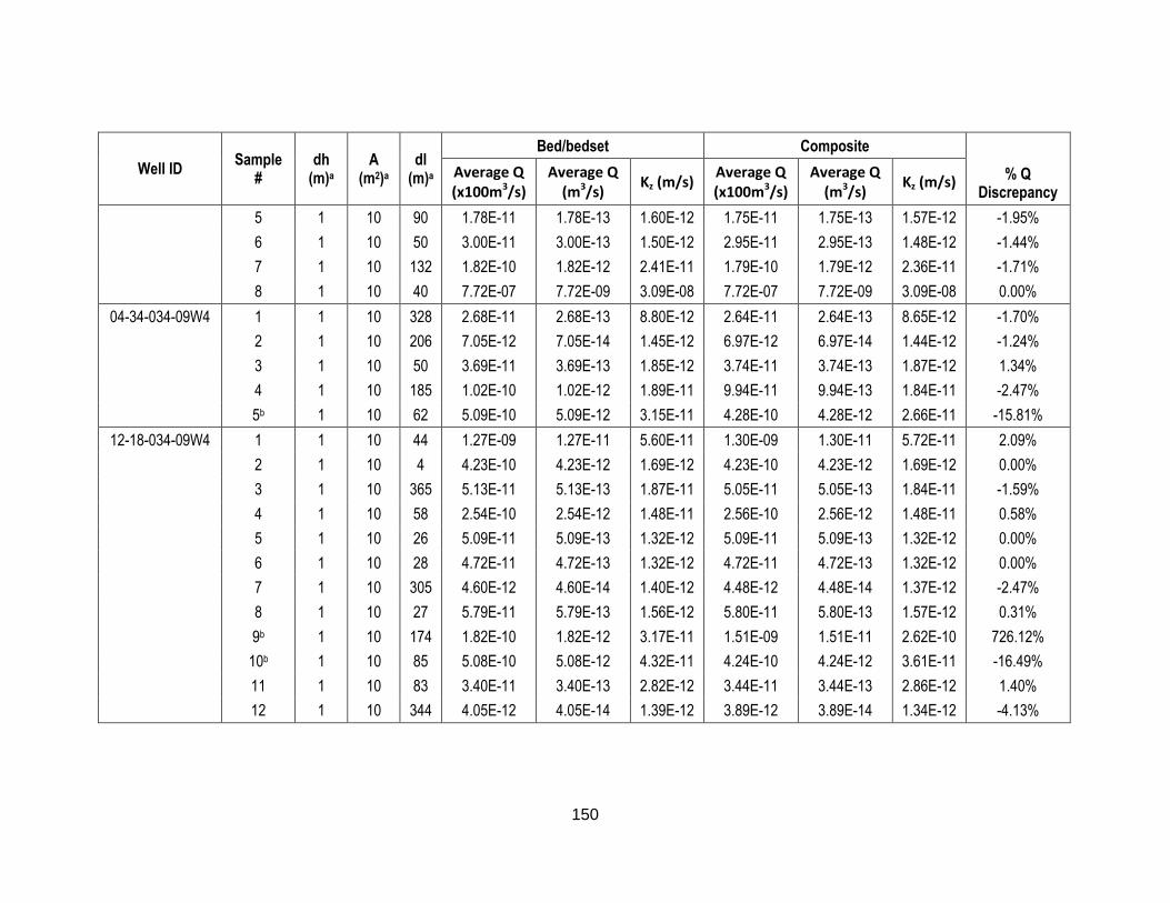
150
Well ID Sample
# dh
(m)a A
(m2)a dl
(m)a
Bed/bedset Composite
% Q Discrepancy
Average Q (x100m3/s)
Average Q (m3/s)
Kz (m/s) Average Q (x100m3/s)
Average Q (m3/s)
Kz (m/s)
5 1 10 90 1.78E-11 1.78E-13 1.60E-12 1.75E-11 1.75E-13 1.57E-12 -1.95%
6 1 10 50 3.00E-11 3.00E-13 1.50E-12 2.95E-11 2.95E-13 1.48E-12 -1.44%
7 1 10 132 1.82E-10 1.82E-12 2.41E-11 1.79E-10 1.79E-12 2.36E-11 -1.71%
8 1 10 40 7.72E-07 7.72E-09 3.09E-08 7.72E-07 7.72E-09 3.09E-08 0.00%
04-34-034-09W4 1 1 10 328 2.68E-11 2.68E-13 8.80E-12 2.64E-11 2.64E-13 8.65E-12 -1.70%
2 1 10 206 7.05E-12 7.05E-14 1.45E-12 6.97E-12 6.97E-14 1.44E-12 -1.24%
3 1 10 50 3.69E-11 3.69E-13 1.85E-12 3.74E-11 3.74E-13 1.87E-12 1.34%
4 1 10 185 1.02E-10 1.02E-12 1.89E-11 9.94E-11 9.94E-13 1.84E-11 -2.47%
5b 1 10 62 5.09E-10 5.09E-12 3.15E-11 4.28E-10 4.28E-12 2.66E-11 -15.81%
12-18-034-09W4 1 1 10 44 1.27E-09 1.27E-11 5.60E-11 1.30E-09 1.30E-11 5.72E-11 2.09%
2 1 10 4 4.23E-10 4.23E-12 1.69E-12 4.23E-10 4.23E-12 1.69E-12 0.00%
3 1 10 365 5.13E-11 5.13E-13 1.87E-11 5.05E-11 5.05E-13 1.84E-11 -1.59%
4 1 10 58 2.54E-10 2.54E-12 1.48E-11 2.56E-10 2.56E-12 1.48E-11 0.58%
5 1 10 26 5.09E-11 5.09E-13 1.32E-12 5.09E-11 5.09E-13 1.32E-12 0.00%
6 1 10 28 4.72E-11 4.72E-13 1.32E-12 4.72E-11 4.72E-13 1.32E-12 0.00%
7 1 10 305 4.60E-12 4.60E-14 1.40E-12 4.48E-12 4.48E-14 1.37E-12 -2.47%
8 1 10 27 5.79E-11 5.79E-13 1.56E-12 5.80E-11 5.80E-13 1.57E-12 0.31%
9b 1 10 174 1.82E-10 1.82E-12 3.17E-11 1.51E-09 1.51E-11 2.62E-10 726.12%
10b 1 10 85 5.08E-10 5.08E-12 4.32E-11 4.24E-10 4.24E-12 3.61E-11 -16.49%
11 1 10 83 3.40E-11 3.40E-13 2.82E-12 3.44E-11 3.44E-13 2.86E-12 1.40%
12 1 10 344 4.05E-12 4.05E-14 1.39E-12 3.89E-12 3.89E-14 1.34E-12 -4.13%
Top Related