Upscaling and History Matching of Fractured Reservoirs

Pål Næverlid SævikDepartment of Mathematics

University of Bergen

Modeling and Inversion of Geophysical Data (Uni CIPR)

March 26, 2015

2

Outline

EnKF Simulation

3

Fractured Rocks

What makes fractures different from other heterogeneities?

4

What makes fractures special?

• Dual porosity behaviour• Scale separation issues• Heterogeneities are larger than lab scale• Prior information on fracture geometry may

be available

5

Dual porosity behaviour

6

Scale separation issues

Large faults and fractures may be impossible to upscale

7

Large and small fractures

The distinction between «large» and «small» fractures is determined by the size of the computational cell

8

Prior fracture information

• Core samples• Well logs• Outcrop analogues• Well testing• Seismic data• EM data (?)

9

Fracture parametersRoughnessAperture (thickness)Filler material

Connectivity

Fracture density

Clustering

ShapeSize

10

Common assumptionsFisher distribution of

orientationsPower-law size

distribution

Cubic transmissitivity law:

11

Numerical upscaling

• Flexible formulation• Accurate solution• Slow• Gridding difficulties• May not have sufficient

data to utilize the flexible formulation

12

Analytical upscaling

• Idealized geometry• Fast solution• Easy to obtain

derivatives• Requires statistical

homogeneity• Difficult to link idealized

and true fracture geometry

13

Effective permeability

pinpout

K1

K2

φ1K1 + φ 2K2

pinpout

φ1K1 + φ 2K2

= A·a·K1 + K2

= A·τ + K2

14

Several fracture sets

• Single frac: • Extension:

15

Partially connected fractures

• Snow (1969): • Oda (1985):

16

Percolation theory

• Assumption: All fractures are polygons of equal shape, distributed randomly in space

• Percolation theory tells us that:

– (percolation threshold)

17

Connectivity prediction

• Mourzenko, V. V., J.-F. Thovert, and P. M. Adler (2011)• is calculated from fracture shape, size and

orientation distribution• is slightly shape-dependent

18

Connectivity and spacing

19

Transfer coefficient

• Kazemi (1976):

• Generalization:, where

• Other alternatives also exists

20

Summary: Input and output parameters

Connectivity f

Density A

Transmissitivity τ

Density A

Aperture aFiller material

Permeability K

Porosity φ

Transfer coefficient σ

Orientation

ShapeSize

Clustering

Roughness

21

History matching of fractured reservoirs

EnKF

Simulation

Simulation

22

Integrated upscaling and history matching

Fracture parame tersAd

just

ups

cale

d pa

ram

eter

s

Permea bility, shape factor

Press ure , flow rates

Mismatch

Upscaling

Simulation

Real data

Adju

st fr

actu

re

par

amet

ers

23

Ensemble Kalman Filter update

• Based on Bayes’ formula:

• All distributions are approximated by a Gaussian distribution, and the covariance is defined using the ensemble

• Update formula:

24

Test problem: Permeability measurement

• Single grid cell• Measured permeability: 200 mD ± 20 mD• Expected aperture: 0.2 mm ± 0.02 mm• Expected density: 1 m-1 ± 0.2 m-1

• Randomly oriented, infinitely extending fractures

• Cubic law for transmissitivity

25

Test problem: Permeability measurement

• Resulting upscaling equations:

26

Predicted fracture porosity

27

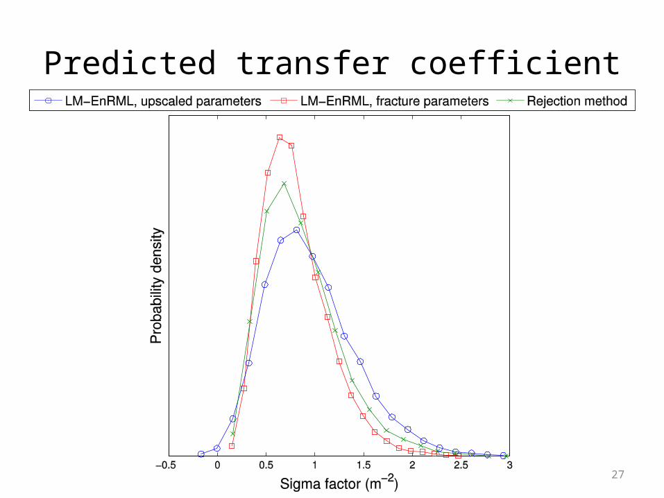
Predicted transfer coefficient

28

Inverse relation and connectivity

• Inverse relation of the upscaling equations

29

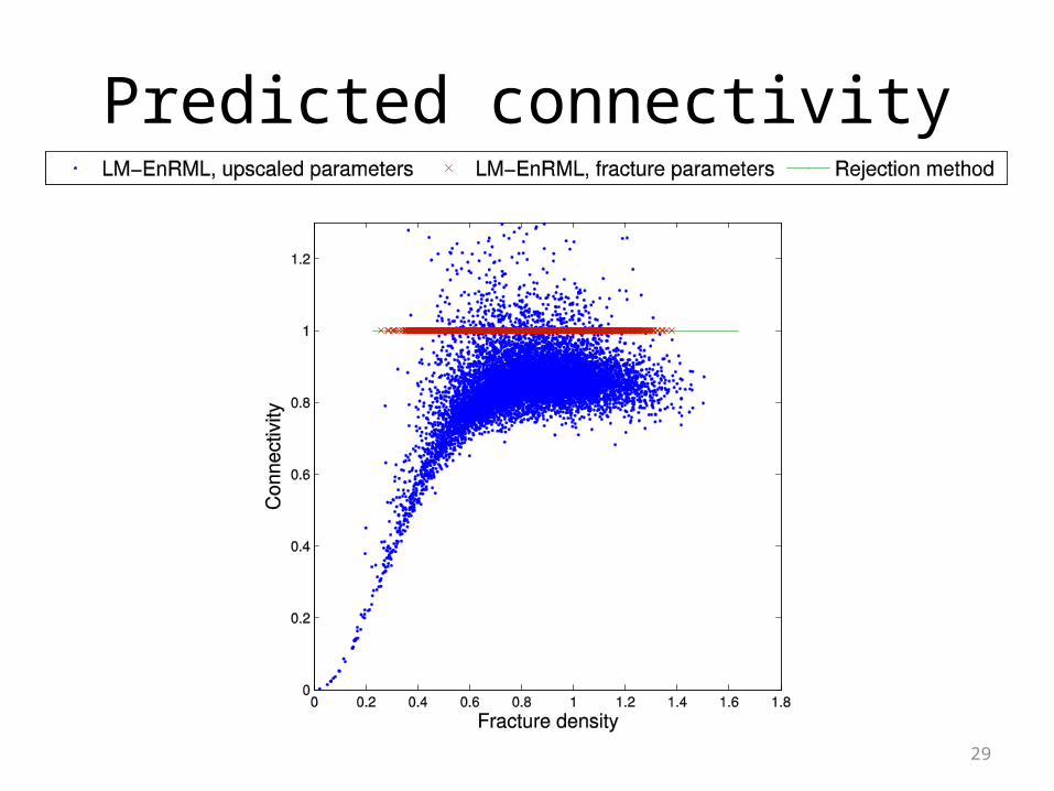
Predicted connectivity

30

Linear fracture upscaling

• Lognormal fracture parameters– Expected log aperture (mm): – Expected log density (m-1):

• Logarithm of the upscaling equation

31

Predicted connectivity

32

Partially connected fractures

• We set fracture size to R = 5 m• Connectivity is computed as

• Connectivity is then a monotonically increasing function of fracture density

33

Predicted connectivity

34

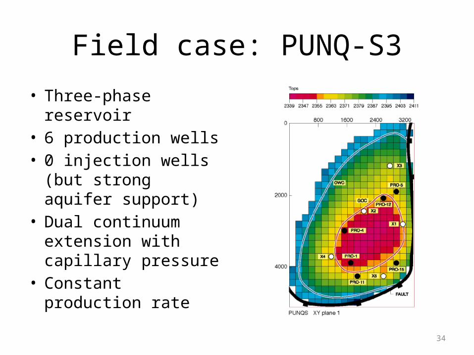
Field case: PUNQ-S3

• Three-phase reservoir• 6 production wells• 0 injection wells (but

strong aquifer support)• Dual continuum

extension with capillary pressure

• Constant production rate

35

Field case: PUNQ-S3

• 2 years of production• 2 years of prediction• Data sampling every

100 days• Data used– GOR– WCT– BHP

• Assimilation using LM-EnRML

36

Data match summaryNumber of LM-EnRML iterations

0 1 2 3 4

Fracture parameters as primary variables

BHP 11.07 3.15 0.99 0.46 0.44

GOR 11.16 5.54 1.38 0.13 0.35

WCT 3.60 0.91 0.90 0.41 0.40

Total 9.31 3.71 1.11 0.37 0.40

Upscaled parameters as primary variables

BHP 11.07 4.78 4.15 4.32 4.42

GOR 11.16 10.26 9.74 9.62 9.65

WCT 3.60 1.26 1.23 1.16 1.21

Total 9.31 6.57 6.15 6.12 6.17

37

BHP,

PRO

-1G

OR,

PRO

-12

WCT

, PRO

-11

Initial ensemble Traditional approach Our approach

38

Perm

eabi

lity

Sigm

a fa

ctor

Initial ensemble Traditional approach

Our approachTrue case

39

Perm

eabi

lity

Conn

ectiv

ity

Initial ensemble Traditional approach

Our approachTrue case

40

Conclusion

• Fracture upscaling creates nonlinear relations between the upscaled parameters

• These relations may be lost during history matching, if upscaled parameters are used as primary variables

• The problem can be avoided by history matching fracture parameters directly