


Languages
Pages
Legal


Effort Estimation
• In WBS ,one can estimate effort (micro-level) but needed to know:– Size of the deliverable
– Productivity of resource in producing that deliverable
Effort = Size / Productivity
e.g. Effort = 500 loc / (100 loc/person-day) = 5 person-days

Effort Estimation (in General)• Has been an “art” for a long time because
– many parameters to consider
– unclear of relative importance of the parameters
– unknown inter-relationship among the parameters
– unknown metrics for the parameters
• Historically, project managers– consulted others with past experiences
– drew analogy from projects with “similar” characteristics
– broke the projects down to components and used past history of workers who have worked on “similar” components; then combined the estimates
For example?
What if you are new at this and have no dependable contacts ?

General (MACRO) Model
• There have been many proposed models for estimation of effort in software. They all have a similar general form:– Effort ≡ (product size) & (other influencing factors)
or more formally
– Effort = [a + (b * ((Size)**c))] * [PROD(f’s)]• where :
– Size is the estimated size of the project in loc or function points
– a, b, c, are coefficients derived from past data and curve fitting
» a = base cost to do business regardless of size
» b = fixed marginal cost per unit of change of size
» c = nature of influence of size on cost
– f’s are a set of additional factors, besides Size, that are deemd important
– PROD (f’s) is the “multiplicative product” of the f’s

COCOMO (macro) Estimating Technique
• Developed by Barry Boehm in early 1980’s who had a long history with TRW and government projects (initially LOC based)
• Later modified into COCOMO II in the mid-1990’s (FP included for size, besides LOC)
• Included process activities :– Product Design – Detailed Design– Code and Unit Test– Integration and Test
• Utilized by some but many people still rely on experience and/or own company proprietary data. (some use COCOMO as a companion estimate)
Note that requirements gathering and spec. are not included

Basic Form for Effort
• Effort = A * B * (size ** C)
• or more “generally”– Effort = [A * (size**C)] * [B ]
– Effort is in “person-months”– A = scaling coefficient – B = coefficient based on 15 parameters– C = a scaling factor for process – Size = delivered source lines of code in “KLOC”

Basic form for Time
• Time = D * (Effort ** E)
– Time = total number of “calendar months”– D = A constant scaling factor for schedule– E = a coefficient to describe the potential
parallelism in managing software development
Past experiences indicate that “time estimate” has usually been more than actual

COCOMO I
• Originally based on 56 projects
• Reflecting 3 modes of projects
– Organic : less complex and flexible process– Semidetached : average complexity project– Embedded : complex, real-time defense
projects

3 Modes are Based on 8 Characteristics
• A. Team’s understanding of the project objective
• B. Team’s experience with similar or related project
• C. Project’s needs to conform with established requirements
• D. Project’s needs to conform with established interfaces
• E. Project developed with “new” operational environments
• F. Project’s need for new technology, architecture, etc.
• G. Project’s need for schedule integrity
• H. Project’s size range
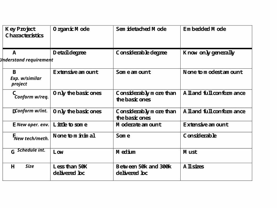
Key Project Characteristics
Organic Mode
Semidetached Mode
Embedded Mode
A Detail degree Considerable degree Know only generally
B Extensive amount Some amount None to modest amount
C Only the basic ones Considerably more than the basic ones
All and full conformance
D Only the basic ones Considerably more than the basic ones
All and full conformance
E Little to some Moderate amount Extensive amount
F None to minimal Some Considerable
G Low Medium Must
H Less than 50K delivered loc
Between 50k and 300k delivered loc
All sizes
Understand requirement
Exp. w/similar project
Conform w/req.
Conform w/int.
New oper. env.
New tech/meth.
Schedule int.
Size

COCOMO I
• For the basic forms:
– Effort = A * B *(size ** C)
– Time = D * (Effort ** E)
• Organic : A = 3.2 ; C = 1.05 ; D= 2.5; E = .38
• Semidetached : A = 3.0 ; C= 1.12 ; D= 2.5; E = .35
• Embedded : A = 2.8 ; C = 1.2 ; D= 2.5; E = .32

Coefficient B
• Coefficient B is an effort adjustment factor based on 15 parameters which varied from very low, low, nominal, high, very high to extra high
• B = product (15 parameters)
– Product attributes:• Required Software Reliability : .75 ; .88; 1.00; 1.15; 1.40; • Database Size : ; .94; 1.00; 1.08; 1.16;• Product Complexity : .70 ; .85; 1.00; 1.15; 1.30; 1.65
– Computer Attributes• Execution Time Constraints : ; ; 1.00; 1.11; 1.30; 1.66• Main Storage Constraints : ; ; 1.00; 1.06; 1.21; 1.56• Virtual Machine Volatility : ; .87; 1.00; 1.15; 1.30;• Computer Turnaround time : ; .87; 1.00; 1.07; 1.15;

Coefficient B (cont.)
• Personnel attributes
• Analyst Capabilities : 1.46 ; 1.19; 1.00; .86; .71;
• Application Experience : 1.29; 1.13; 1.00; .91; .82;
• Programmer Capability : 1.42; 1.17; 1.00; .86; .70;
• Virtual Machine Experience : 1.21; 1.10; 1.00; .90; ;
• Programming lang. Exper. : 1.14; 1.07; 1.00; .95; ;
• Project attributes
• Use of Modern Practices : 1.24; 1.10; 1.00; .91; .82;
• Use of Software Tools : 1.24; 1.10; 1.00; .91; .83;
• Required Develop schedule : 1.23; 1.08; 1.00; 1.04; 1.10;

An example
• Consider an averag e(semidetached) project of 10Kloc:
– Effort = 3.0 * B * (10** 1.12) = 3 * 1 * 13.2 = 39.6 pm
– Where B = 1.0 (all nominal)
– Time = 2.5 *( 39.6 **.35) = 2.5 * 3.6 = 9 months
– This requires an additional 8% more effort and 36% more schedule time if we include product plan and requirements:
• Effort = 39.6 + (39.6 * .08) = 39.6 + 3.16 = 42.76 pm• Time = 9 + (9 * .36) = 9 +3.24 = 12.34 months
Any problem?
Try another example
• Go through the assessment of 15 parameters for the effort adjustment factor, B.
• You may have some concerns :
– Are we interpreting each parameter the same way– Do we have a consistent way to assess the range of
values for each of the parameters– -How good is my size (loc) estimate?

COCOMO II
• Effort performed at USC with many industrial corporations participating
• Has a database of over 80 some projects
• “Early” estimate, preferred to use Function Point instead of LOC for size; “later” estimate may use LOC for size. (loc is harder to estimate without some experience)
• Coefficient B based on 15 parameters for early estimate is “rolled” up to 7 parameters, and for late estimates use 17 parameters.
• Scaling factor for process has 6 categories ranging in value from .00 to .05, in increments of .01

Function Point A non-LOC based estimator
• Often used to assess software “size” and “complexity”
• Started by Albrecht of IBM in late 1970’s

Function Point an estimation of “size”
• LOC as an estimate of “size” has many drawbacks but still used because of physical analogy:
– Different programming languages has different loc meaning
– Measures source code which is not available until implementation phase; it so hard to estimate during early phases of project

FP Utility
• Where is FP used?
– Comparing software in a “normalized fashion” independent of op. system, languages, etc.
– Benchmarking and “Projection” based on “size”: • size -> effort or cost• size -> development schedule• size -> defect rate
– Outsourcing Negotiation

Function Point
• Provides you a way to estimate the size* of the project based on estimating (items from requirements & high level design):– Inputs– Outputs– Inquiries– Files– Interfaces
• After getting the size, then --- still need to have an estimate on productivity and other factors to get effort in person-months:– productivity in: function-point/person-month– ** *Divide the estimated total project function points by the
productivity to get an estimate of person-month or person-days needed.***
Functional/Transaction related
Data related

Function Point (FP) Computation
• Composed of 5 “Primary Factors”– Inputting items (external input items from user or another application)
– Outputting items (external outputs such as reports, messages, screens – not each data item)
– Inquiry (a query that results in a response of one or more data)
– Master and logical files (internal file or data structure or data table)
– External interfaces (data or sets of data sent to external devices, applications, etc.)
• And a “complexity level index” matrix : Simple Average Complex
Input
Output
InquiryLogical files
Interface
3 4 64 5 73 4 67 10 155 7 10

Function Point Computation (cont.)
1. Initial Function Point :
– ∑ (# of Primary Factor (i) x Complexity Level Index for i)
2. There are 14 more “Degree of Influences” ( 0 to 5 scale) :• data communications
• distributed data processing
• performance criteria
• heavy hardware utilization
• high transaction rate
• online data entry
• end user efficiency
• on-line update
• complex computation
• reusability
• ease of installation
• ease of operation
• portability
• maintainability

Function Point Computation (cont.)
• Define Technical Complexity Factor (TCF):
– TCF = .65 + (.01 x DI )
– where DI = ∑ ( influence factor values)
• So note that .65 < TCF < 1.35
• Function Point (FP) = Initial FP x TCF

What’s one Function Point?
• Do you have any experience in converting say ----- 35 function points to effort in person months?
• Is there any standard conversion factor that you may use? – In IBM, during 90s, about 20 function points to 1
person month of effort (this was back in late 1990’s --- may be more productive now).
Top Related