UNIVERSITY OF HERTFORDSHIRE

Faculty of Engineering and Information Sciences

MCOM0177 Computer Science MSc Project (Online)

Final Report

January 2013

Software Effort Estimation using Artificial Intelligence

Clinton Mercieca

Operational Programme II – Cohesion Policy 2007 - 2013 Empowering People for More Jobs and a Better Quality Life

Scholarship part-financed by the European Union European Social Fund (ESF)

Co-financing rate: 85% EU Funds; 15% National Funds

Investing in your future

1

Contents

Abstract ...................................................................................................................................... 3

Acknowledgements .................................................................................................................... 4

1. Introduction ........................................................................................................................... 5

1.1 Background ....................................................................................................................... 5

1.2 Problem Description & Methodology .............................................................................. 5

1.3 Thesis Structure ................................................................................................................ 7

2. Software Effort Estimation Methods ..................................................................................... 8

2.1 Expert Estimation ............................................................................................................. 8

2.2 Formal Estimation Models ............................................................................................... 9

2.2.1 Size-based Models ..................................................................................................... 9

2.2.2 Parametric Models ................................................................................................... 10

2.2.3 Analogy-based Estimation ....................................................................................... 10

2.3 Choice of estimation method ......................................................................................... 11

3. Artificial Intelligence ............................................................................................................ 12

3.1 Artificial Neural Networks .............................................................................................. 12

3.2 Fuzzy Logic ...................................................................................................................... 14

3.3 Genetic Algorithms ......................................................................................................... 15

3.3.1 Encoding................................................................................................................... 15

3.3.2 Crossover ................................................................................................................. 16

3.3.3 Mutation .................................................................................................................. 17

3.3.4 Fitness ...................................................................................................................... 17

3.4 Choice of Artificial Intelligence Technique ..................................................................... 18

4. Enhancing COCOMO with the use of Genetic Algorithm ..................................................... 19

4.1 Tools & Technologies used ............................................................................................. 19

4.1.1 Effort Estimation Method ........................................................................................ 19

4.1.2 Development Tools .................................................................................................. 19

4.1.3 Data Storage ............................................................................................................ 20

4.1.4 Development Methodology ..................................................................................... 20

4.2 Design ............................................................................................................................. 20

4.3 Implementation .............................................................................................................. 22

4.3.1 User Interface .......................................................................................................... 22

4.3.2 Encoding/Decoding .................................................................................................. 22

4.3.3 Population ................................................................................................................ 23

2

4.3.4 Parent Selection ....................................................................................................... 23

4.3.5 Crossover ................................................................................................................. 24

4.3.6 Mutation .................................................................................................................. 24

4.3.7 Fitness Calculation ................................................................................................... 24

4.4 Sample Dataset ............................................................................................................... 25

4.5 Results ............................................................................................................................ 26

4.6 Conclusion ...................................................................................................................... 29

5. Conclusion ............................................................................................................................ 30

5.1 Limitations ...................................................................................................................... 30

5.2 Further Work .................................................................................................................. 31

5.2.1 Software Effort Estimation ...................................................................................... 31

5.2.2 Optimisation of Effort Estimation using AI .............................................................. 32

Bibliography ............................................................................................................................. 33

Appendixes ............................................................................................................................... 36

Appendix A: Encode/Decode ................................................................................................ 36

Appendix B: Parent Selection ............................................................................................... 37

Appendix C: Crossover .......................................................................................................... 38

Appendix D: Fitness Function ............................................................................................... 39

3

Abstract

Being able to define the projected cost and duration of a project during the early stages of project management has been a sought after activity for many years. Throughout the years many methodologies and models have been created to help in this field; however some degree of accuracy still eludes. In this thesis, we will explore some of the most popular methods that are used to provide management with software effort estimation values. We will also review some Artificial Intelligence (AI) technologies which can be used to achieve more accurate effort estimation. Then in order to provide with proof on the use of AI within an effort estimation model, the basic Constructive Cost Model (COCOMO) effort estimation technique was used together with a genetic algorithm. The algorithm was developed solely with the purpose of optimising the variable parameters used within the effort estimation model’s formula. The results obtained from the artefact produced were able to provide with proof that artificial intelligence can provide with a considerable improvement in accuracy.

4

Acknowledgements

First and foremost I would like to thank my supervisor, Dr Renato Amorim for his support and prompt feedback whenever I needed it. His guidance and advice was a very valuable asset in the completion of this thesis.

Also my gratitude goes to Dr Maria Schilstra, the MSc Project module leader, and also Dr Wei Ji, their feedback and presence in the online class discussions was highly appreciated.

I am also grateful for the support which my friends, family and loved ones provided during the period I spent working on this project. Their words of encouragement helped me to keep going onwards whenever I felt unmotivated during the hard times.

Finally I would like to thank all those lecturers and fellow students who have been part of my post-graduate studies.

The research work disclosed in this publication is partially funded by the Strategic Educational Pathways Scholarship Scheme (Malta). The scholarship is part-financed by the European Union – European Social Fund.

5

1. Introduction

1.1 Background According to a market research on Information Technology (IT) projects, performed by Dynamic Markets [1], the three main issues related to projects within the IT industry are time overruns, budget overruns and more than expected costs involved when maintaining software. All three problems can be attributed to project management; however the source of the problem for time and budget overruns resides in shortcomings during Software Effort Estimation. Effort estimation is performed at an early stage during the software project lifecycle, usually after all the requirements for the project have been gathered. The estimate can be the result of various techniques which can be used in order to try and foresee the work which the project will entail. Through this estimation, the management can then allocate resources and time for the project to be carried out and completed. The challenge involved in this task is quite a difficult one, since it is very hard to predict the challenges that certain tasks will involve, especially if these types of tasks are being performed for the first time. Furthermore there is a certain degree of psychological pressure involved in this kind of estimates, since the project success or failure may very well depend on it.

1.2 Problem Description & Methodology How can AI be used in conjunction with Parametric Software Effort Estimation

Models in order to obtain more accurate estimates when compared with a

conventional Effort Estimation Model?

This is the research question that this master’s thesis will answer. The objective of the work presented in this thesis is to find a method by which the burden of the software effort estimation process can be eased, through the possibility of automating the estimation by use of an already existing model. An Artificial Intelligence (AI) technology is combined with an estimation model in order to find out whether an AI algorithm can enhance the model and therefore produce more accurate results.

Therefore, the core objectives of this thesis are:

• Review existing literature on parameterised software estimation models and give a critical evaluation in relation to the possibility of integrating artificial intelligence as an aid in order to obtain more realistic results

• Review existing literature on different types of artificial intelligence algorithms and give a critical evaluation in order to identify the best candidate for integration with a parameterised software effort estimation model.

• Design and develop a software prototype that implements the two techniques previously chosen from the literature review.

6

• Using a predefined dataset of project values, run the prototype and extract results to be compared with the actual data from the dataset used, in order to produce a comparative result.

• Evaluate the results obtained and draw conclusions based on those results.

In addition to the above, the following advanced objectives have been set

• Provide a means by which users can input actual results to be fed into the system, so that the system can use this data to ‘learn’ and therefore be able to produce more accurate results

• Enable the users to select different estimation models by which the system can then output the result

• Allow the users to customise different weightings for different parameters within the AI algorithm

In order to reach the defined objectives, the project is split into two phases, a research task which explores existing literature regarding software effort estimation models and AI, and another more practical phase which produces a prototype that combines the two technologies and delivers the results to demonstrate the findings obtained. The research part consists mainly of reviewing and analysing already existing literature and works on the two topics in question. The software application is built using .Net technologies and a Waterfall development methodology. The final conclusions derived from the work done provide an answer to the research question posed at the start of this project.

7

1.3 Thesis Structure This thesis consists of four chapters. The first chapter is a brief introduction which presents the reader with a short background together with the research question and objectives for the thesis. The second and third chapters consist of the literature research and review on existing material. Chapter two contains a review of different software effort estimation methods including expert estimation and different formal estimation models, from which an effort estimation model is then chosen as one of the tools in the thesis practical work. Chapter three reviews different technologies in AI, including artificial neural networks, fuzzy logic and genetic algorithms, which provides the knowledge to choose the second medium through which the final results of this thesis can be achieved. Chapter four provides details on the combination of the software effort estimation model and the AI technology, chosen from chapters 2 and 3, in order to create a software application artefact that can optimise the software effort estimation model chosen. The final chapter summarises the results obtained, presents conclusions upon those results and provides suggestion for further work on the subject together with an evaluation of the project as a whole.

8

2. Software Effort Estimation

Methods

In project management several models and practices exists when the effort involved in a software project needs to be calculated. These methods are subdivided in the following categories [2]:

• Expert estimation

• Formal estimation models

• Estimation methods which make use of a combination of more than one method

Each category presents with a different approach to software effort estimation having its pros and cons.

2.1 Expert Estimation Expert estimation is the most commonly used estimation method for calculation of software projects effort [3]. Expert estimation consists of producing an estimate based on personal experience in the field of work. Due to this, the methodology can be either more or less accurate or totally off target, mostly depending on the individual or individuals performing the estimation. In order for a process to be considered as an expert estimation method, it has to be performed by an individual who is considered an expert in the field and most of the process is based on his experience and intuition, some would even say gut feeling. As it can be expected, estimation may vary depending on the estimator, since different individuals will have different levels of expertise and experience in the field of work. However there are a few practices and principles which may support experts in order to avoid human bias on the final estimate. As explained by M. Jørgensen [3] these are:

1. Evaluate estimation accuracy, but avoid high evaluation pressure – Expert estimation places the estimator at the centre of the estimation process, therefore this may result in a high amount of pressure induced over the individual, especially in large projects in which failure could be severely punished. A balance should be reached where the estimator should feel motivated but at the same time he or she should not experience excessive pressure induced by the task.

2. Avoid conflicting estimation goals – most often when trying to estimate the effort involved in a software project, the estimator finds himself trying to balance between trying to issue estimates as low as possible in order to place a desirable offer to the client and establish a cost which will also profit the company. This type of conflict sometimes leads to inaccurate effort estimates.

3. Ask the estimators to justify and criticize their estimates – the exercise of justification and self-criticism of estimates may provide the estimator with a different view on how the software should be developed and therefore improve the estimation process.

9

4. Avoid irrelevant and unreliable estimation – An expert performing an estimate should be trained in filtering out information regarding the system which is irrelevant to the estimation process or which may not be accurate. This is especially crucial when revising software requirements and client expectations.

5. Use documented data from previous development tasks – Previously carried out tasks always provide with a good hint on estimation of similar tasks. However attention must be paid to task which were not documented, since recollection of effort involved in a task from personal memory can be misleading in the estimation process and lead to under or overestimation.

6. Find estimation experts with relevant domain background and good estimation

record – it is important to distinguish between an expert and a novice. An expert has a certain degree of experience in his field of work and is more likely to make accurate estimates than an individual with the same academic level but with less experience [4]

Even given the guidelines above, the research performed by M. Jørgensen [3] still suggests that expert estimation still provides no significant advantage in performance over other estimation models, and it is far from being an exact science, since it relies over human expertise. However this methodology may be utilised as a valuable aid in conjunction with other estimation methodologies in order to produce more accurate effort predictions.

2.2 Formal Estimation Models Formal effort estimation models are methods which employ a fixed methodology in order to estimate effort. They may consist of a formula, function or other method which has been obtained through the study of previous actual project results and which can now be employed in the same way to provide estimation for the project which is submitted to the estimation model. Formal estimation models need an input which most of the time is based on size or other effort related value, which then the model would use in order to calculate effort by means of a regression process [6]. The main advantage of these models is the fact that they are not subject to influence by the individual using them due to their formality and strict method of use.

2.2.1 Size-based Models Size-based methods rely on finding the size of the project. Two models in this category are Function Points and Use Case Points, Function Points being the more popular of the two. Both methods are based on deriving a measure based on the requirements of a software project.

The function points method involves splitting the different functionality in the software in different classes and give weights to the different functionalities. The results are then added and processed through a formula to obtain the final function points value [9]. This value is then used to extract effort estimation or can further be processed through the formula [10]

LOC = a * UFC + b

10

Where parameters a and b are values extracted from regression of already completed projects. The value in lines of code (LOC) can then be further used for effort estimation purposes. The main advantage of function points is that the value can be calculated at an early stage, since the only prerequisite to be able to extract the function points value is the project requirements. Even so, studies [9][10] have shown that no satisfactory margin of success could be obtained when using this method of estimation, or rather the model was not superior to any other type of effort estimation. However function points are still a useful tool to size-up a software project and could be used in conjunction with other models in order to possibly produce more reliable results in effort estimation.

2.2.2 Parametric Models Parametric models consist of formula based functions which accept a number of parameters related to a project in order to calculate the effort value needed in order to carry out that project. Several different models exist which classify under this category, some of which are Software Lifecycle Management (SLIM), Software Evaluation and Estimation of Resources – Software Estimating Model (SEER-SEM) and Constructive Cost Model (COCOMO) which was later revised to establish the COCOMO II model. The most renown of the models mentioned above is COCOMO, mainly due to its simplicity. The basic COCOMO model formula consists of the following [8]:

MM = a * KDSI b

Where MM denominates the result in Man Months which is a measure of the effort needed, KDSI stands for thousands of delivered source instructions or lines of code and parameters a and b are variables which are determined depending on the type of project [8].

This kind of models provide with a structured and simpler way how to calculate the software effort needed to complete a project, however they are highly inflexible. A model formula may provide an accurate estimate for a type of project, while it would fail to do the same for a similar project. Boehm [8] states that COCOMO is ideal for extraction of rough estimates, since it lacks to consider factors like hardware availability, personnel quality and other factors which cannot be taken into consideration by the inclusion of a few parameters.

Even with their lack of flexibility, some estimation models, Like COCOMO II are quite complex and can cater for different phases of the project lifecycle and different factors that can affect the project [8]. Of course the more complex the parametric model the more specialised, the personnel using the model need to be, since unlike expert estimation, parametric models present with a more technical approach to estimation.

2.2.3 Analogy-based Estimation The word analogy is defined as “a comparison between one thing and another, typically for the purpose of explanation or clarification” [15], and analogy-based estimation methods are based on that premise. If two different projects share the same attributes, then the effort involved in completing them should be similar to one another. Analogy-based estimation derives estimation values by comparing the

11

target project to historical data from similar projects which have already been completed [11]. In order to do so, the first step in this type of estimation is to derive the features that define the project to be estimated, and then the project is compared to already complete projects in a historical database. Once a project with high similarity is found in the historical database, then the effort estimation value can be derived by mitigating for differences between the two projects [13]. This type of estimation can be rather accurate and considered more trustworthy than other estimation methods due to the fact that the estimation is based on recorded historical facts, however analogy-based estimation has also a few issues and prerequisites. The estimator must first of all have access to a comprehensive database of documented previous projects, which most companies do not maintain and it is a rather difficult task to classify projects and their features within a historical database. Also if no closely related project is found in the database, then effort estimation will either be impossible to produce or be rather inaccurate. Given these shortcomings, analogy-based estimation can still be a reliable tool [14], especially when combined with other technologies like Fuzzy logic and neural networks, when compared to other estimation techniques.

2.3 Combination-based Estimation Methods Combination-based estimation methods, as the name suggests involves the use of both a formal estimation model and expert estimation. This is a more realistic approach to estimation, where after a formal effort estimation model works out the effort needed for a project, the resulting value is adjusted by an experienced individual in order to try and provide with a more realistic prediction for the effort the project will entail. In a way, the formal estimation model provides a hint for the final answer.

2.4 Choice of estimation method For the purpose of this thesis an estimation method was chosen to be the subject of this study. As mentioned previously, expert estimation is the most used estimation method, however it is far too human dependent and almost impossible to apply any form of automation to it due to the human intuition factor involved in it. On the other hand a formal estimation method denotes a form of conformity to a predefined methodology when calculating the effort estimation value. This proved to be ideal when trying to automate the process and applying artificial intelligence to the process. In the literature review presented, three different formal methodologies were identified. Of the three, parametric models, was chosen due to the fact that they follow a predefined formula which then is made more flexible by the inclusion of one or more parameters. These parameters can be the subject for fine tuning by means of artificial intelligence so as to provide more accurate effort estimation. From all the parameterised models, COCOMO was used due to its simplicity, which should also provide with a clearer understanding of the benefits resulting from the application of artificial intelligence to the effort estimation method.

12

3. Artificial Intelligence

In order to optimise the software effort estimation process, another technology will be combined with an effort estimation model. The human input can be a valuable asset for an estimation methodology, in order to get a more accurate result; however, it would take a long time for a human being to take into consideration several factors that affect the prediction. Also there is no guarantee that the final result is an accurate one due to various factors that distinguish one estimator from another, like expertise, experience or common sense. In order to try to emulate the input that a human being would give to an effort estimation model, artificial intelligence (AI) will be used.

The main function of AI is to introduce an element of intelligence to whichever system it is applied by means of a man-made computational medium [16]. In this section we review some of the possible AI technologies which can be employed with a parameterised effort estimation model, so as to optimise the final result.

3.1 Artificial Neural Networks An Artificial Neural Network (ANN) is an information processing framework that was designed by taking the human brain as an inspiration to how it works. Like the human brain, an ANN is composed of several small information processing modules called neurons, all connected to each other. Every neuron can process the data which it is supplied from different sources and produce one output, which then is forwarded to other neurons. When supplied with input data, the neuron will have a set of rules which determine whether the neuron should fire or not depending on the input pattern it receives. If the neuron receives a patter for which it was not instructed upon, it will compare the data received to the firing instructions it has and if the pattern has a predominant similarity to one of the instructions, the firing rule is applied to that pattern. If the neuron is still undecided after comparing the pattern to the instructions, none of the rules is applied. This architecture enables an ANN to learn as more data is inputted into it, since every time data is processed through it, new results can be derived. This process is called Generalisation [17].

The learning process is perhaps the most important feature within an ANN. This process can be classified in two different categories, supervised and unsupervised [19]. During a supervised training process, existing labelled data is supplied to the neurons; this enables the neurons to tweak the weightings within the ANN, therefore accelerating the learning process. On the other hand, an unsupervised training process will not supply any additional data except the one used as the starting input and will leave the ANN to adapt itself and output a result.

The architecture within most common ANNs consists of three layers; the input layer, the hidden layer and the output layer. In the input layer, data is collected and fed into the network to the hidden layer. Neurons in the input layer can also apply weights to the initial data; this allows a degree of control on which neurons will fire. Within the hidden layer, neurons will process the data through their connections and

13

weights. Within the hidden layer the neurons can be interconnected in two different ways. The simpler ANNs would be connected in a feedforward way, which means that data can only travel in a single direction. On the other hand when using a feedback pattern, the hidden layer can implement loops and therefore send data in different directions. Feedback networks are much more powerful than feedforward due to their flexibility and tend to get extremely complex. Once data passes through the hidden layer, it is forwarded to the output layer to apply further weights and issue the final result.

Figure 1: Feedforward ANN [17]

Figure 2: Feedback ANN [17]

Due to their learning capabilities, artificial neural networks have been used in many sectors, including marketing, risk management, financial and even medicine [20]. However in order to implement an ANN a large amount of data input is required

14

especially when trying to solve a complex problem, since the more data the network is fed, the more it can learn and therefore the more useful and effective it will be. Also, a complex ANN could become highly resource hungry on the machine it runs upon, consuming large amounts of disk space and memory. These shortcomings often lead projects to move away from the application of ANNs. Still the field remains in the spotlight for the academic area due to its fascinating nature and potential for future applications, especially in robotics [22].

3.2 Fuzzy Logic Fuzzy logic is an approximation system that can be applied to problems which have multiple input parameters. The human brain is capable of deriving answers based on approximate data, while conventional machine algorithms deal in absolutes or binary logic. The objective of fuzzy logic is to mimic the human reasoning based on the non-absolute data that it is provided. Where binary logic uses values zero and one, to describe a state, fuzzy logic uses the whole spectrum from zero to one which can be represented as a decimal value or perhaps a percentage.

The first thing to establish within a fuzzy logic algorithm is the membership sets. Membership sets determine whether an input value belongs to a set or not. These set may overlap, which represents the degree of transition between one set and another, for example, there is no clear cut of when a temperature is cold and when it is hot, but instead there are several other temperature states in between the absolutes. In a simple graphical representation, the set would be drawn as area graphs one overlapping the other as shown in figure three. The shape of the graphs can vary according to the requirements and case being examined.

Figure 3: Membership sets graphs

0

20

40

60

80

100

120

0 100

%

Temperature

Cold

Warm

Hot

15

In order to determine in which membership set or sets a value belongs, a membership function for each membership set is defined. Through the membership function, a fuzzy graph can be extracted against a set of rules which will then produce the final result. Once the membership functions are evaluated against the defined system rules, the mathematical centroid for the fuzzy graph is calculated and the final result is achieved. This example only covers the simplest of the cases related to fuzzy logic. More complex systems would include several inputs and the internal mathematical functions can get rather complex [23].

Today fuzzy logic systems are being introduced in many areas, including industrial automation, common appliances, military applications [24] and also the film industry [25] amongst many others. Even though fuzzy logic systems are being introduced, there are still arguments against it. One of which is the fact that number of rules within a fuzzy system will increase exponentially inverse to the accuracy level [26]. Also a fuzzy system will need to be calibrated manually since there is no learning process involved like we have seen earlier in neural networks. Even so, fuzzy logic systems still remain a fascinating topic and as demonstrated by its day to day applications, also a very reliable one.

3.3 Genetic Algorithms While Artificial Neural Networks and Fuzzy Logic are based on how the human brain processes data, a Genetic Algorithm (GA) is based on the concept of biological evolution, discovered by Charles Darwin. In order to understand the concept of genetic algorithms, first we need to look into what inspired it. Biological evolution can be defined as the slow change at a DNA level of a life form. That DNA then dictates the changes in growth and development of an individual. This process normally effects a large population, as they reproduce through several generations. Change occurs due to mixing of genes from the parents of an individual and/or random mutation, both of which can either produce a stronger or a weaker offspring [27].

A genetic algorithm works in the same way as an evolutionary process. The core components of a genetic algorithm are the following:

• Encoding

• Crossover

• Mutation

• Fitness

Following is a brief explanation of each one of these components [28] [29].

3.3.1 Encoding Encoding refers to the process by which the data related to the problem which needs to be solved, is translated in a format which the genetic algorithm can understand and process to try to find a solution. Once the data is encoded, a dataset will be produced. This dataset is described as a chromosome. In biology a chromosome is DNA configuration and therefore a chromosome within a genetic algorithm can also be a possible solution to the problem being tackled. Several techniques exist to

16

perform the encoding process, including binary encoding, permutation encoding, value encoding and tree encoding.

3.3.2 Crossover The Crossover is the process responsible for the generation of a new chromosome from already existing ones. It is the biological equivalent of two individuals producing an offspring. In order to choose which individuals from the population will be used to produce the new offspring, different processes and techniques can be used. The selection method can be as simple as choosing random individuals to mathematical operations in order to ensure that mating chromosomes are strategically selected. Once the chromosomes have been selected, the crossover process can commence. Again, there are various methods by which the crossover can happen, some of which are the following:

Single Point Crossover – both parents are split in two at a randomly selected location within the chromosome and the two sections in the chromosomes are exchanged so as to create new offsprings.

Multi-Point Crossover – similar to single point crossover, but the splitting locations are more than one

Uniform Crossover – genes are copied within the offspring chromosome according to a randomly generated mask which determines which genes are taken from which parent.

Three Parent Crossover – genes are copied to the offspring according to a specific pattern. If the respective gene in the first parent is the same as the one in the second parent, then that gene is copied to the offspring, else the corresponding gene from the third parent is copied.

Crossover with Reduced Surrogate – ensures that an offspring is always different from its parents, by examining the parents beforehand in order to determine the crossover point to produce an original offspring.

Shuffle Crossover – genes are copied as in a uniform crossover, but before copying, genes, the parents are shuffled with a single-point crossover.

Precedence Preservative Crossover (PPX) – a mask is used to determine from which parent genes are taken, however genes are taken sequentially depending on which gene is next in the parent and ignoring genes which have already been drawn from that parent. This ensures that gene precedence is always maintained.

Ordered Crossover – every parent is split in three, similar to a two-point crossover; a first child inherits the left and right part of the first parent. The middle section is determined by the order in which the genes are found in the second parent. A similar process is applied for a second child based on the second parent

Partially Matched Crossover (PMX) – this type of crossover is usually used when working with integers as genes. The parents are split with a two-point crossover. A matching section is swapped between the two parents. At this point, the resulting

17

chromosomes may have duplicate values. Each child is legalized by replacing the duplicates within the unswapped sections with the missing values.

It should be noted that during a single iteration within a genetic algorithm, even though two parents are chosen there is a chance that crossover does not happen. This is represented by a parameter which dictates the probability that two chromosomes are subject to a crossover.

3.3.3 Mutation Similar to biological evolution, a genetic algorithm incorporates a slight chance that a chromosome is subject to a mutation. The role of mutation is that of including an aspect of random change within the process. This process does not necessarily produce a beneficial effect, but it can replenish lost chromosomes patterns as well as producing completely new ones. The probability of a mutation to occur is normally much lower than that of a crossover. The process of mutation normally is carried out by one of the following methods:

• Flipping bits within a chromosome from zero to one or vice versa

• Interchanging the positions of two bits within the chromosome

• Reversing the bits next to a randomly chosen position

3.3.4 Fitness Fitness is what determines how successful a chromosome is at solving the problem at hand. A fitness function is normally closely related to the problem that the genetic algorithm is trying to solve and therefore cannot be reused for different problems. It also determines which chromosomes are passed to the next population within an iteration of the algorithm, when using a survival of the fittest scenario and whether the target objective has been reached.

Once all these elements are combined, the genetic algorithm will be able to build a whole population of chromosomes, by first encoding chromosomes, selecting parents from the current population and perform crossovers and mutations to create new offsprings which will build a new population. The process is repeated until an individual chromosome within a population fits the predefined criteria that defines whether the problem is solved or not, most of the time dictated by the fitness function.

Genetic Algorithms are particularly used for optimization problems and can explore a wide variety of solutions, since there is no limit to how many populations the algorithm can produce. A high grade of reusability can be obtained from a genetic algorithm, not accounting for the fitness function, unlike Fuzzy Logic and neural Networks which must be designed specifically to tackle a problem. Even so, certain tuning must happen before reusing a genetic algorithm, which means setting the population size, crossover and mutation probability [29]. The stronger advantage of this type of algorithms remains that of providing a robust algorithm by which multiple solutions can be explored and mapped to a real-world problem.

18

3.4 Choice of Artificial Intelligence Technique In order to integrate Artificial Intelligence (AI) within an effort estimation method, one AI technology needed to be chosen from the three that were explored during the research phase of this project. The first AI technique that was explored was neural networks, which would serve as an optimiser for COCOMO; however it would need a large amount of starting data in order to learn and evolve to optimise the model. Since the project dataset to be used in this project is not that extensive, neural networks would not be a wise decision, since the project could come at a halt due to lack of data to feed the neural network. On the other hand, Fuzzy Logic does not need a large amount of starting data to work, however the technology can become highly reliant on mathematical background and overly complicated which could result in a stand still within the project. The last AI technology explored within this project is the most feasible option, since genetic algorithms are mostly used for optimisation problems, which is exactly what is needed for this project; also they can present us which a large amount of solution options, while still being rather flexible in their implementation.

19

4. Enhancing COCOMO with the use

of Genetic Algorithm

In order to prove the value that AI can contribute to achieve a more accurate effort estimation in software development projects, a software application has been built that uses a genetic algorithm in order to optimise the parameters used within the basic COCOMO model.

4.1 Tools & Technologies used In this section, all the tools and technologies which were used to produce the software artefact will be included together with the reasons behind the choice of that medium.

4.1.1 Effort Estimation Method As mentioned before, the software effort estimation method used to demonstrate the findings using the prototype built was the basic COCOMO. The reasoning behind this choice lies mainly in the fact that COCOMO is one of the most popular parameterised effort estimation methods and also the fact the formula is so simple that it lets us place more focus on the variance parameters rather than on an overtly complicated formula. The formula used to test the software artefact is the one shown below:

MM = a * KDSI b

The formula contains two variable parameters labelled a and b which can be optimised. Once defined, the two parameters can then be used within the formula together with the amount of delivered source instructions which is measured in thousands (KDSI). The calculated result is the effort needed which is measured in man months (MM). This formula is the focus within the software application to demonstrate the use of AI to optimise effort estimation.

4.1.2 Development Tools The main development tool used to create the AI prototype was the .Net Framework. The main reason behind using this development tool was the familiarity and previous experience with programming in .Net languages, especially C#, which was the language used to code the software artefact. However other advantages are brought to the table by the .Net Framework, including high code readability, reliability and toolsets which are already in place and easy to use. The fact that the framework has readymade functions like Random functions and Mathematical functions have accelerated considerably the development process and helped in delivering a more reliable software prototype. The integrated development environment (IDE) used to code the application was Microsoft Visual Studio 2010.

20

4.1.3 Data Storage In order for the prototype to operate and produce data that can be later examined, some sort of data storage needed to be used in conjunction with the software application. The medium that was determined as ideal for the purpose of this project was Extensible Markup Language (XML). The choice was motivated by a number of reasons; the most influencing was the fact that to use XML there was no need for further setup of third-party applications, unlike when using a database. Also the project did not need for any complex data storage means, so a relational database has been deemed unnecessary. XML is also highly readable through a simple text document or even web browser and therefore can be examined outside of the application, if need be. In this case, data storage through XML was used in order to store the actual projects’ dataset used within the genetic algorithm and also to store results which are extracted from the algorithm while it is operating. The results can then be opened directly as an excel sheet that can be interpreted and processed to produce meaningful data. The .Net framework also provides very efficient libraries, through which XML can be read and manipulated easily without excessive development, therefore making data reading and storage fast and reliable.

4.1.4 Development Methodology Since the prototype application is a relatively small piece of software, there was no need to use any complex development methodology; therefore the methodology chosen for the development of the genetic algorithm prototype was the waterfall model. As the waterfall model dictates, the development stage involved, listing of Requirements, Design, Development and finally Testing. Every stage was followed by the next one and in between documents were produced, some of which consisted of list of features, design flowcharts and various notes which in turn have been used to produce the documentation to follow.

4.2 Design During the design phase, a general idea of the operation of the prototype was defined. This involved two main areas which would make up the main parts within the genetic algorithm’s application. The first design phase involved designing the flow that the algorithm will take from start to end, with generic stages which could then be further developed. As illustrated in Figure 4, the process will start by generating a random chromosome population and calculating the fitness for each member of the population. This will be the starting point on which the algorithm will then improve. Even if highly unlikely, it can occur that the target fitness is reached with the first randomly generated population, at which point the application will stop the algorithm and report the results. If not, the algorithm will go on to populate the next population of chromosomes, by first choosing the best chromosomes from the current population, referred to as the elitists, and moving them to the next population group. The rest of the population is created as shown in Figure 5 below.

The first step in creating a new chromosome is to choose the parents from which the new chromosome will be produced. Then it is determined whether crossover between the parents will happen, if so, the crossover process is performed and the new chromosome is generated. If crossover does not happen, a random parent is

21

taken from those chosen and moved to the new population. In addition to crossover, there is a slight chance of a mutation to happen within the chromosome. Once the mutation is performed, the chromosome is ready to be moved to the new population. This process will continue to repeat until the new population is filled up.

Once a population is complete, the system will check whether any fitness rating within the population satisfies the objective fitness or the maximum amount of tries available to obtain the objective fitness has been reached, at which point the application will report the results.

Figure 4: GA Process flowchart

Figure 5: Population process flowchart

22

4.3 Implementation This section covers a more in depth description of all the vital parts within the genetic algorithm application.

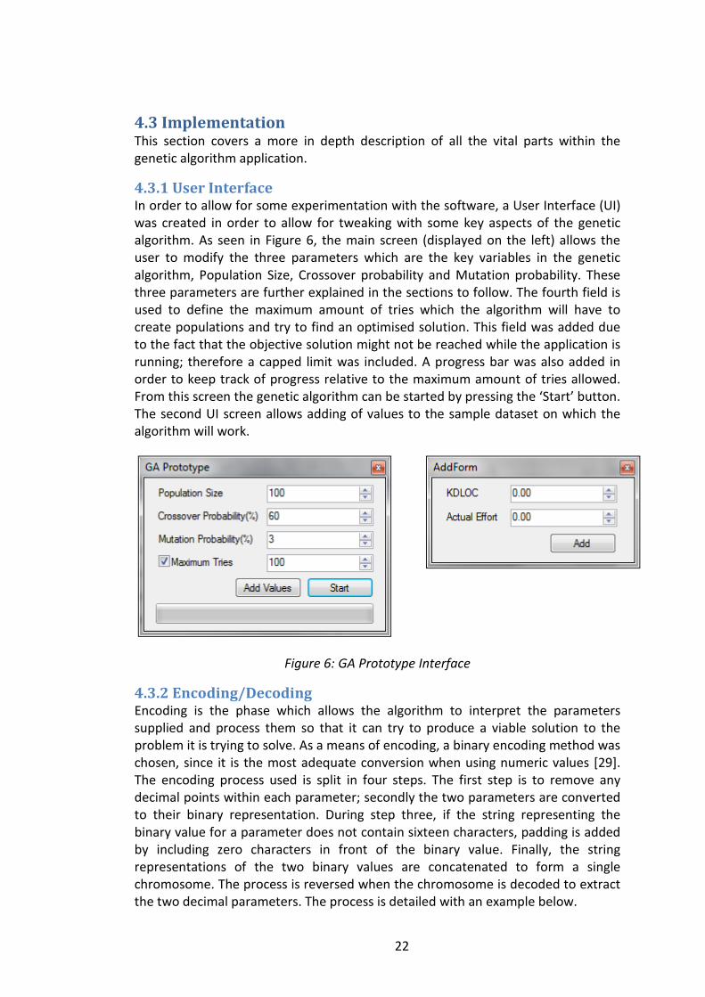
4.3.1 User Interface In order to allow for some experimentation with the software, a User Interface (UI) was created in order to allow for tweaking with some key aspects of the genetic algorithm. As seen in Figure 6, the main screen (displayed on the left) allows the user to modify the three parameters which are the key variables in the genetic algorithm, Population Size, Crossover probability and Mutation probability. These three parameters are further explained in the sections to follow. The fourth field is used to define the maximum amount of tries which the algorithm will have to create populations and try to find an optimised solution. This field was added due to the fact that the objective solution might not be reached while the application is running; therefore a capped limit was included. A progress bar was also added in order to keep track of progress relative to the maximum amount of tries allowed. From this screen the genetic algorithm can be started by pressing the ‘Start’ button. The second UI screen allows adding of values to the sample dataset on which the algorithm will work.

Figure 6: GA Prototype Interface

4.3.2 Encoding/Decoding Encoding is the phase which allows the algorithm to interpret the parameters supplied and process them so that it can try to produce a viable solution to the problem it is trying to solve. As a means of encoding, a binary encoding method was chosen, since it is the most adequate conversion when using numeric values [29]. The encoding process used is split in four steps. The first step is to remove any decimal points within each parameter; secondly the two parameters are converted to their binary representation. During step three, if the string representing the binary value for a parameter does not contain sixteen characters, padding is added by including zero characters in front of the binary value. Finally, the string representations of the two binary values are concatenated to form a single chromosome. The process is reversed when the chromosome is decoded to extract the two decimal parameters. The process is detailed with an example below.

23

Decimal parameters 4.5011 0.6216

Remove decimal point 45011 6216

Convert to binary 1010111111010011 1100001001000

Padding of missing zero’s 1010111111010011 0001100001001000

Concatenation 10101111110100110001100001001000

The code methods used to encode and decode chromosomes within the genetic algorithm can be viewed in Appendix A.

4.3.3 Population The population size is one of the variable factors within the genetic algorithm. This can be set by the user through the application’s UI. A larger population will allow the application to explore a wider range of possible solutions, since more different chromosomes will be produced and will allow for a wider selection of parents for generation of new chromosomes. Larger populations also help to avoid premature convergence to the problem solutions which normally occurs when the chromosomes within a population fail to create new chromosomes which improve over their predecessors and therefore not improving over the problem’s solution. During the results investigation stage, premature convergence to the parameter optimisation solution was encountered, since processing and memory limitations from the processing machine could not permit for extremely high population values or running the algorithm for more than a few hours before the machine would slow down due to lack of memory resources. However a final set of parameters could always be extracted so results could still be obtained from the algorithm.

In order to start creating a population, a starting point needed to be established. In the prototype application the first iteration of the chromosome population is created at random by generating two random numbers to represent the two separate parameters within the equation. The random number can range between 0.0001 and 6.5535. The parameters are then encoded to create the chromosome. This process is repeated until the population is filled.

4.3.4 Parent Selection Parent selection is the process by which two or more parents are selected so that they can be used in the creation of new chromosomes. For this phase of the genetic algorithm, two methods were considered, one being a roulette wheel selection [31], where parents with higher fitness are more likely to be picked as parents than others with lower fitness. When implementing this type of parent selection, a problem was found due to the fact that the .Net randomisation function was unable to generate a random number within the range that could pick parents which have a very low fitness. This resulted in some of the chromosomes never getting the chance to be selected as parents, even if their chance for selection was very small. After this problem was discovered, another parent selection method was considered, known as binary tournament selection [31]. Binary tournament selection involves selecting two chromosomes at random from the current population, then picking the chromosome with the best fitness from the two of them. This process is then repeated for each parent that needs to be selected. This method is ideal for the parent selection process since it both involves a random

24

factor and fitness is taken into consideration, while giving a chance for every chromosome to be selected. The parent selection code method can be examined in Appendix B.

4.3.5 Crossover In order to produce new offspring chromosomes, a crossover process between two or more parent had to be chosen. As mentioned before, there is no guarantee that the crossover process will happen for every chromosome generated, which is governed by the crossover probability that the user will set. In a previously mentioned section, several crossover methods were reviewed; from those uniform crossover was chosen. In order to perform a uniform crossover, a mask is produced every time a crossover needs to be performed. The mask is then used to determine which genes will be picked from which parent. There is an equal probability to pick a gene from either parent, which in our case is a 50% probability, since the crossover is done using two parent chromosomes. After the mask is created, genes are picked from the two parents according to the mask in order to generate the new chromosome.

The reasoning behind this choice lies in the fact that uniform crossover possesses a balance between complexity and efficiency. Uniform crossover provides with a good recombination process to produce new chromosomes which is more effective than a fixed point crossover since the contribution from parents is done at gene level rather than with whole segments, while still preserving common genes positions from parents. Also the randomisation of the mask that maps the crossover process has a certain degree of assurance that a child generated from two parents will be different if the crossover between the same two parents happens again. The crossover process code can be viewed in Appendix C.

4.3.6 Mutation Mutation is the process by which a genetic algorithm tries to exploit wider solution options. The rate at which the mutation process happens is also governed by the mutation probability which can be set from the application’s user interface in order to make it easier to explore different solutions when running the application. Specific to the case being tackled by this project, the mutation process happens by inverting two genes within a chromosome. The genes are selected at random from within the thirty two binary values within a chromosome string.

4.3.7 Fitness Calculation The fitness function within the genetic algorithm can be considered the heart of the application. The fitness function will determine whether a chromosome is fit enough to be promoted to the next generation, whether a chromosome is fit enough to become the parent for another chromosome and whether or not the genetic algorithm has reached the target fitness. The fitness rating of the chromosomes within a population is also used to keep track of the improvements done by the genetic algorithm while it is iterating and creating new populations. Therefore we see how vital this aspect of the algorithm is. In order to create the fitness function, a dataset of actual data was needed to be able to compare results derived from chromosomes. This dataset is further discussed in the next section.

25

The fitness function developed for this project consists of a comparison function which calculates the difference between the parameters represented by a chromosome applied to the basic COCOCMO formula and the actual results of a project from within the sample dataset. The process begins by retrieving the dataset from the XML file repository. The parameters supplied to the fitness function are then used, together with the amount of lines of code from the dataset, in the basic COCOMO formula stated earlier to obtain the effort estimation. This is done for each project within the dataset. The effort estimates are then compared with the actual project effort values to obtain a variance value from the actual results as a percentage. Finally the average difference from the actual values is calculated and returned as the fitness rating for that chromosome. Since the value returned by the function is a measure of difference, the lower the value returned, the more fit a chromosome will be. The code segment that calculates the fitness rating for a chromosome can be viewed in Appendix D.

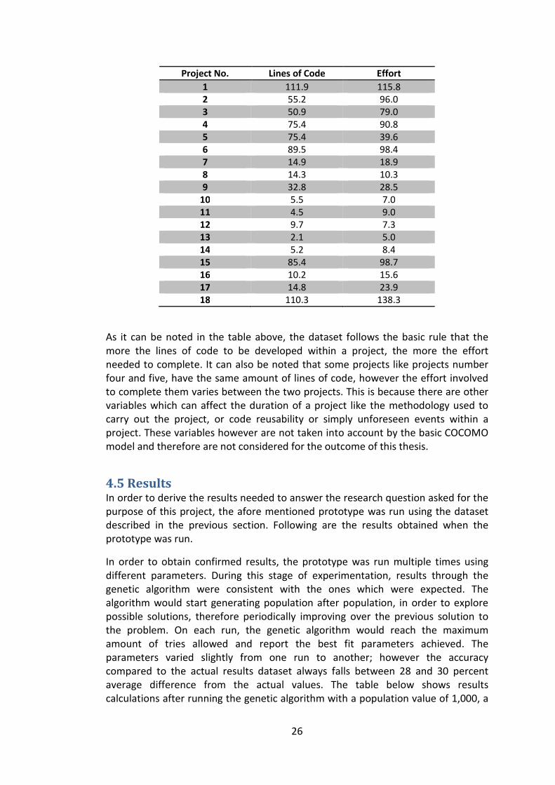
4.4 Sample Dataset The sample dataset which was used in this project consists of a list of eighteen projects for which there is actual recorded data. The dataset was first used in a study carried out by J. Bailey and V. Basili [32] and was further used by others in similar studies. The dataset consists of a number of variable parameters recorded for completed projects; however in this project only two of the recorded values were used. The data used is the size of the project which is measured in thousands of lines of code and the actual effort that that was involved in the project to complete, which is measured in man-months. The dataset can be seen in the table below.

26

Project No. Lines of Code Effort

1 111.9 115.8 2 55.2 96.0 3 50.9 79.0 4 75.4 90.8 5 75.4 39.6 6 89.5 98.4 7 14.9 18.9 8 14.3 10.3 9 32.8 28.5

10 5.5 7.0 11 4.5 9.0 12 9.7 7.3 13 2.1 5.0 14 5.2 8.4 15 85.4 98.7 16 10.2 15.6 17 14.8 23.9 18 110.3 138.3

As it can be noted in the table above, the dataset follows the basic rule that the more the lines of code to be developed within a project, the more the effort needed to complete. It can also be noted that some projects like projects number four and five, have the same amount of lines of code, however the effort involved to complete them varies between the two projects. This is because there are other variables which can affect the duration of a project like the methodology used to carry out the project, or code reusability or simply unforeseen events within a project. These variables however are not taken into account by the basic COCOMO model and therefore are not considered for the outcome of this thesis.

4.5 Results In order to derive the results needed to answer the research question asked for the purpose of this project, the afore mentioned prototype was run using the dataset described in the previous section. Following are the results obtained when the prototype was run.

In order to obtain confirmed results, the prototype was run multiple times using different parameters. During this stage of experimentation, results through the genetic algorithm were consistent with the ones which were expected. The algorithm would start generating population after population, in order to explore possible solutions, therefore periodically improving over the previous solution to the problem. On each run, the genetic algorithm would reach the maximum amount of tries allowed and report the best fit parameters achieved. The parameters varied slightly from one run to another; however the accuracy compared to the actual results dataset always falls between 28 and 30 percent average difference from the actual values. The table below shows results calculations after running the genetic algorithm with a population value of 1,000, a

27

crossover probability of 95% and a mutation probability of 5%. The parameters obtained using this configuration were 1.6387 and 0.9052 as parameters a and b respectively, so obtaining the effort estimation formula below.

MM = 1.6387 * KDSI 0.9052

Using the formula, the following result comparison was derived.

Project No. Lines of Code Actual Effort GA Result %age Difference

1 111.9 115.8 117.247 1.2 2 55.2 96.0 61.845 35.6 3 50.9 79.0 57.467 27.3 4 75.4 90.8 82.016 9.7 5 75.4 39.6 82.016 107.1 6 89.5 98.4 95.783 2.7 7 14.9 18.9 18.9 0 8 14.3 10.3 18.21 76.8 9 32.8 28.5 38.607 35.5

10 5.5 7.0 7.668 9.5 11 4.5 9.0 6.394 29 12 9.7 7.3 12.815 75.6 13 2.1 5.0 3.208 35.8 14 5.2 8.4 7.288 13.2 15 85.4 98.7 91.803 7 16 10.2 15.6 13.412 14 17 14.8 23.9 18.785 21.4 18 110.3 138.3 115.728 16.3

Average %age

Difference

28.76

During other runs using different population, crossover and mutation values, results were very similar to the ones above, with only minimal variations on the overall average percentage difference rating. However, it was noted that at higher population capacity, the genetic algorithm would take more iterations in order to converge to a stable result, which conforms to what was expected from a genetic algorithm of this sort. The charts below in figures 8 and 9 show fitness progress tracking for two different runs of the genetic algorithm up until convergence using a population value of 1,000 and 10,000. As already stated previously, as the fitness improves, the fitness value will decrease. Convergence happened twice as fast when using a lower population amount, which leaves less time for the algorithm to explore possible solutions. Also, higher populations show a more gradual improvement in the fitness of chromosomes, after the first random population, unlike smaller populations which improve drastically at fewer points as it can be seen happening around iterations 2 and 7 when using a population of 1,000 chromosomes. This may hinder diversity within the population chromosomes and therefore limit future improvements for finding a solution.

28

Figure 8: Fitness progression using a population amount of 10,000

Figure 9: Fitness progression using a population amount of 1,000

In order to compare results with the conventional basic COCOMO, effort estimation was worked out using the suggested parameter values below [8].

Project Type/Parameter a b

Organic 2.4 1.05

Semi-detached 3 1.12

Embedded 3.6 1.20

Since through the dataset used, we have no knowledge of the project type, every data record was worked out using all three parameter sets and the most accurate result was taken. The following data table was obtained.

27.5

28

28.5

29

29.5

30

30.5

31

1 3 5 7 9 11 13 15 17 19 21 23 25 27 29 31 33 35 37 39 41

Fitness

Fitness

29.06

29.08

29.1

29.12

29.14

29.16

29.18

29.2

29.22

29.24

29.26

1 2 3 4 5 6 7 8 9 101112131415161718192021

Fitness

Fitness

29

Project

No.

Lines of

Code

Actual

Effort

Result %age

Difference

Parameter

Types Used

1 111.9 115.8 289.003 149.6 Organic 2 55.2 96.0 137.615 43.3 Organic 3 50.9 79.0 126.382 60 Organic 4 75.4 90.8 190.928 110.3 Organic 5 75.4 39.6 190.928 382.1 Organic 6 89.5 98.4 228.583 132.3 Organic 7 14.9 18.9 34.792 84.1 Organic 8 14.3 10.3 33.322 223.5 Organic 9 32.8 28.5 79.671 179.5 Organic

10 5.5 7.0 12.218 74.5 Organic 11 74.5 9.0 16.17 79.7 Semi-

detached 12 9.7 7.3 22.169 203.7 Organic 13 2.1 5.0 4.446 11.1 Organic 14 5.2 8.4 11.52 37.1 Organic 15 85.4 98.7 217.601 120.5 Organic 16 10.2 15.6 23.37 49.8 Organic 17 14.8 23.9 34.547 44.5 Organic 18 110.3 138.3 284.665 105.8 Organic

Average %age

Diff.

222.58

4.6 Conclusion While the results obtained from the genetic algorithm cannot be denied, the development process in order to produce the artefact proved to be a challenging one. Every aspect of it had to be planned in advance and catered specifically to fit the problem that the project is trying to solve, especially the coding and decoding of chromosomes and also the fitness function. These aspects of the software application have a very low degree of reusability. Also a lot of experimentation had to be done in order to extract data from the AI application so as to find the optimum setup. Even so, the genetic algorithm approach proved to be a feasible route for optimisation of parameters within the basic COCOMO model, as the resulting data suggests.

30

5. Conclusion

After analysing the data extracted from the genetic algorithm and comparing it with the data obtained when using the conventional basic COCOMO approach, it can be clearly observed that estimates calculated using parameters obtained from the genetic algorithm provide for a more reliable effort estimation than that of the standard parameter values suggestions. The difference in accuracy proved to be more than marginal, since results obtained during the course of this study showed that values resulting from the use of AI were at least seven times more accurate than those obtained using a standard effort estimation model. Even though these results were specific to a chosen set of data, it cannot be denied that AI could be a valuable asset to be incorporated within the software effort estimation field. It should also be stated that the success of AI related to software effort estimation is highly dependable upon the implementation which is specific to the effort estimation method that is used, like in this case, encoding of chromosomes, fitness function, and other parts within the genetic algorithm. These aspects contribute highly to the results as does the quality and size of the sample dataset which is used to evaluate the fitness of chromosomes within the algorithm.

Even given the improvement in accuracy, AI still is not a perfect tool for software effort estimation. When examining results at individual project level, shortcomings for specific projects could still be found, sometimes overestimating effort for a project by more than hundred percent. This is still unacceptable in a software development business environment, where overshooting of estimates of this kind can lead to great financial losses. Therefore up until now, the human judgment still cannot be eliminated completely from this part of the project management phase.

5.1 Limitations The data results obtained from the genetic algorithm, compared to the conventional basic COCOMO were very encouraging, however as effort estimation goes, there are several limitations which constrict the effectiveness of the approach used.

The first limitation to mention must be the effort estimation model itself, the basic COCOMO model is one of the most basic parametrical models and therefore lacks to take into consideration factors like software development methodologies used, code reusability, developers’ skill, and other factors which affect the outcome of the effort estimation model. This could be clearly seen when working out effort estimates results for projects number four and five in the results table. These projects have the same amount of lines of code, however project number five took much less effort to complete. This could have been due to a high rate of code reusability or any other factor which could have improved the effective completion time of the project.

Another limitation that was encountered was hardware limitations while running the genetic algorithm. Even though the software application is not very resource

31

hungry in itself, the amount of iterations and large amount of data generation, can occupy quite the amount of resources on a machine. During experimental runs of the algorithm, the maximum amount of iterations that could be performed using a high population rating, were five hundred. These proved enough to converge for a satisfying result, however given more resources, the algorithm may have generated more accurate results as it could generate more populations with more chromosomes in them to explore more possibilities.

5.2 Overall Project Evaluation At the beginning of this project, a set of objectives were set, which can be reviewed in Chapter 1. These objectives were essential in order to establish to which degree, the material provided in this thesis satisfies the outcomes which were previously set. By the end of the study, the core objectives which were set have been successfully met. However not all advanced objectives could be met. Unfortunately due to time constraints within the project, the genetic algorithm could not be adapted to operate with different effort estimation models. This could have provided with an interesting comparative study of how well AI interacts with different models, therefore this objective has been included in the Further Work chapter, as a next step in future studies to follow.

Apart from objectives, a project plan with delivery dates was set so as to help in keeping work and deliverables on track. The project plan can be found in Appendix E. With respect to actual delivery dates, the phase that took longer than expected was the Research and Literature Review which had a one week overrun. However the phases which followed in the project plan were able to compensate for this unexpected lateness.

As an overall evaluation, the project has contributed greatly to personal knowledge both in the field of Software Effort Estimation and Artificial Intelligence and I will be looking forward to expand my knowledge in both subjects through further study.

5.3 Further Work The work presented in this thesis holds the potential to be further expanded in future studies. The field of software effort estimation is constantly being the target of new studies due to its importance in the early stages of project management. The practical work contained in this thesis has been carried out specifically concerning genetic algorithms and the basic COCOMO effort estimation model. In this section, the various aspects on which further studies can be conducted are discussed.

5.3.1 Software Effort Estimation The basic COCOMO model used as the target of the software artefact of this thesis, however, the model itself is quite old and new versions of it have been released [8] which may provide with more accurate estimations and therefore could also be the target for improvement with artificial intelligence. A more in detail study could be carried out by comparing multiple parameterised models when optimised using different artificial intelligence technologies.

32

5.3.2 Optimisation of Effort Estimation using AI Even though a genetic algorithm was used for this study, the AI techniques reviewed within this thesis together with others can be used to avail the improvement of software effort estimation. There have already been studies [14] which used Fuzzy logic to improve the accuracy of effort estimation, which is proof that the field is vast enough to conduct further in detail studies on the subject.

33

Bibliography

[1] Dynamic Markets Limited, 2007. IT Projects: Experience Certainty. [Online] Available at: http://www.tcs.com/Insights/Documents/independant_markets_research_report.pdf [Accessed on 2nd September 2012]

[2] M. Jørgensen & M. Shepperd, 2007. A Systematic Review of Software

Development Cost Estimation Studies. [Online] Available at: http://simula.no/research/se/publications/Jorgensen.2007.1/simula_pdf_file [Accessed on 11th September 2012]

[3] M. Jørgensen (2004) ‘A review of studies on expert estimation of software

development effort’ The Journal of Systems and Software. 70 (2004) pp. 37-60

[4] C. Jarabek. Expert Judgement in Software Effort Estimation. [Online] Available at: http://people.ucalgary.ca/~cjjarabe/papers/expertJudgment.pdf [Accessed on 12th September 2012]

[5] M. Jorgensen, B. Boehm, S. Rifkin (2009) ‘Software Development Effort

Estimation: Formal Models or Expert Judgment?’ Software, IEEE. 26 (2) pp. 14-19

[6] J. Živadinović, Z. Medić, D. Maksimović, A. Damnjanović, S. Vujčić, 2011.

Methods of Effort Estimation in Software Engineering. [Online] Available at: http://www.tfzr.uns.ac.rs/emc2012/emc2011/Files/F%2003.pdf [Accessed on 21st September 2012]

[7] National Aeronautics and Space Administration, 2007. Basic COCOMO. [Online] Available at: http://cost.jsc.nasa.gov/COCOMO.html [Accessed on 23rd September 2012]

[8] M. Glinz, A. Mukhija, 2003. COCOMO (Constructive Cost Model). [Online] Available at: https://files.ifi.uzh.ch/rerg/arvo/courses/seminar_ws02/reports/Seminar_4.pdf [Accessed on 23rd September 2012]

[9] R. Meli, L. Santillo, ‘Function Point Estimation Methods: a Comparative

Overview’, in FESMA ’99 Conference proceedings, Amsterdam, 4-8 October, 1999.

[10] F. Niessink, H. Van Vliet, ‘Predicting Maintenance Effort with Function Points’, in ICSM ’97 Conference proceedings , Bari, Italy, 28 September-2 October 1997.

[11] H. Leung, Z. Fan, 2001, ‘Software Cost Estimation’, in Handbook of Software

Engineering and Knowledge Engineering

[12] M. Chemuturi. Analogy based Software Estimation. [Online] Available at: http://www.chemuturi.com/Analogy%20based%20Software%20Estimation.pdf [Accessed on 1st October 2012]

34

[13] J. Li , R. Conradi, 2007. Issues of Implementing the Analogy-based Effort

Estimation in a Large IT Company. [Online] Available at: http://www.idi.ntnu.no/grupper/su/publ/li/space2007-apsec.pdf [Accessed on 1st October 2012]

[14] M. Azzeh, Software Project Effort Estimation By Analogy, PhD thesis, University of Bradford, UK. [Online] Available at: http://bradscholars.brad.ac.uk/bitstream/handle/10454/4442/PhD%20Thesis_Mohammad%20Azzeh.pdf?sequence=2 [Accessed on 4th October 2012]

[15] Oxford Dictionaries. [Online] Available at: http://oxforddictionaries.com/definition/english/analogy?q=analogy [Accessed 4th October 2012]

[16] I. S. N. Berkeley, 1997. What is Artificial Intelligence? [Online] Available at: http://www.ucs.louisiana.edu/~isb9112/dept/phil341/wisai/WhatisAI.html [Accessed on 10th October 2012]

[17] C. Stergiou, D. Siganos. Neural Networks. [Online] Available at: http://www.doc.ic.ac.uk/~nd/surprise_96/journal/vol4/cs11/report.html [Accessed on 12th October 2012]

[18] R. Calabretta, A. Di Ferdinando, D. Parisi (2004) ‘Ecological neural networks for

object recognition and generalization’ Neural Processing Letters. 2004 (19) pp. 37-48

[19] P. Makhfi (2004). Introduction to Neural Networks. [Online] Available at: http://www.makhfi.com/tutorial/introduction.htm [Accessed on 10th October 2012]

[20] G. Caocci, R. Baccoli, G. La Nasa (2011). The Usefulness of Artificial Neural

Networks in Predicting the Outcome of Hematopoietic Stem Cell Transplantation, Artificial Neural Networks - Methodological Advances and Biomedical Applications, Prof. Kenji Suzuki (Ed.), ISBN: 978-953-307-243-2,InTech, [Online] Available at: http://cdn.intechopen.com/pdfs/14891/InTech-The_usefulness_of_artificial_neural_networks_in_predicting_the_outcome_of_hematopoietic_stem_cell_transplantation.pdf [Accessed on 12th October 2012] [21] M. Azizinezhad, M. Azizinezhad (2011) ‘Langusage, Translation and Neural Networks: Obstacles and Limitations’ Academic Research International. 2011 vol. 1, no. 3, pp. 115-124

[22] N. Dingle (2011). Artificial Intelligence: Fuzzy Logic Explained. [Online] Available at: http://www.controleng.com/home/single-article/artificial-intelligence-fuzzy-logic-explained/8f3478c133.html [Accessed on 15th October 2012]

[23] J. Yen (1999) ‘Fuzzy Logic-A Modern Perspective’ IEEE Transactions on Knowledge and Data Engineering. 1999 vol. 11, no. 1, pp. 153-165

35

[24] B. Klingenberg, P. F. Ribeiro. Fuzzy Logic Applications. [Online] Available at: http://www.calvin.edu/~pribeiro/othrlnks/Fuzzy/apps.htm [Accessed on: 15th October 2012]

[25] A. Lakhani, Multi-agent Systems in Massive, MSc thesis, Bournemouth University [Online] Available at: http://nccastaff.bournemouth.ac.uk/jmacey/Massive/Amit/finished_thesis.pdf [Accessed on 17th October 2012]

[26] J.L. Castro (1999). ‘The limits of fuzzy logic’ Mathware & Soft Computing. 1999 no.6, pp. 155-161 [Online] Available at: http://ic.ugr.es/Mathware/index.php/Mathware/article/viewFile/231/207 [Accessed on 17th October 2012]

[27] F. Traina (2009). What is Biological Evolution. [Online] Available at: http://evolutionedu.org/2009/08/18/what-is-biological-evolution/ [Accessed on: 19th October 2012]

[28] M. Obitko (1998). Genetic Algorithms. [Online] Available at: http://obitko.com/tutorials/genetic-algorithms/ [Accessed on: 20th October 2012]

[29] S. N. Sivanandam, S. N. Deepa (2008) Introduction to genetic algorithms, Springer, New York

[30] RC Chakraborty (2010). Fundamentals of Genetic Algorithms. [Online] Available at: http://www.myreaders.info/09_Genetic_Algorithms.pdf [Accessed on 20th October 2012]

[31] R.Sivaraj, T.Ravichandran (2011) ‘A Review of Selection Methods In Genetic

Algorithm’ International Journal of Engineering Science and Technology. 2011 vol. 3, no. 5, pp. 3792-3797

[32] J. Bailey, V. Basili (1981) ‘A Meta-Model for Software Development Resource

Expenditure’ in Fifth International Conference on Software Engineering, 1981.

[33] M. Glinz, A. Mukhija, ‘COCOMO(Constructive Cost Model)’, in Seminar on Software Cost Estimation WS 2002/2003, Requirements Engineering Research Group, Department of Computer Science, University of Zurich, Switzerland, 3 December 2002.

36

Appendixes

Appendix A: Encode/Decode

public static string Encode(decimal param1, decimal param2)

{ param1 = Math.Round(param1, 4);

param2 = Math.Round(param2, 4);

//Convert to whole numbers

int iParam1 = Convert.ToInt32(param1 * 10000);

int iParam2 = Convert.ToInt32(param2 * 10000);

//Convert to binary

string sparam1 = Convert.ToString(iParam1, 2);

string sparam2 = Convert.ToString(iParam2, 2);

string param1Result = sparam1;

string param2Result = sparam2;

//Add front padding if needed

for (int i = 0; i < (16 - sparam1.Length); i++) param1Result = param1Result.Insert(0, "0");

for (int j = 0; j < (16 - sparam2.Length); j++) param2Result = param2Result.Insert(0, "0");

return param1Result + param2Result;

}

public static decimal[] Decode(string chromosome)

{ //separate strings for the two parameters

int midpoint = chromosome.Length / 2;

string chromo1 = chromosome.Substring(0, midpoint);

string chromo2 = chromosome.Substring(midpoint, midpoint);

//Convert from binary to integers and then //to decimal by dividing to include the decimal point

int iParam1 = Convert.ToInt32(chromo1, 2);

int iParam2 = Convert.ToInt32(chromo2, 2);

decimal[] dParams = new decimal[2];

dParams[0] = Math.Round(Convert.ToDecimal(iParam1) / 10000, 4);

dParams[1] = Math.Round(Convert.ToDecimal(iParam2) / 10000, 4);

return dParams;

}

37

Appendix B: Parent Selection

private List<int> ChooseParents(int parentCount,

List<double> itemsFiteness, Random

rand) {

List<int> parents = new List<int>();

List<double> fitnessList = new List<double>(itemsFiteness);

/// Iterates for the number of parents which are needed

for (int i = 0; i < parentCount; i++) {

int contender1 = rand.Next(0, itemsFiteness.Count);

int contender2 = -1;

do

{

contender2 = rand.Next(0, itemsFiteness.Count); } while (contender1 == contender2);

if (itemsFiteness[contender1] < itemsFiteness[contender2]) parents.Add(contender1);

else

parents.Add(contender2); }

return parents;

}

38

Appendix C: Crossover

public static string Crossover(string parent1, string parent2)

{

string child = "";

//Create crossover mask

bool[] mask = new bool[32];

Random r = new Random();

for (int i = 0; i < mask.Length; i++)

if (r.Next(0, 100) < 50)

mask[i] = true;

//Build new chromosome by selecting from parents according to mask

for (int i = 0; i < 32; i++)

{ if (mask[i])

child += parent1[i];

else child += parent2[i];

}

return child;

}

39

Appendix D: Fitness Function

public static double CalculateFitness(decimal[] parameters)

{

List<double> paramsEstimates = new List<double>();

//Work out the Effort estimate using the COCOMO formula with the

//parameters from the chromosome foreach (ProjectInfo pi in ProjectsData)

{

double estResult = Math.Pow(pi.KDLOC, Convert.ToDouble(parameters[1]));

estResult = estResult * Convert.ToDouble(parameters[0]);

paramsEstimates.Add(estResult);

}

double totalDiff = 0;

double actualTotal = 0;

//Calculate the percentage difference from all the actual effort

values

for (int i = 0; i < ProjectsData.Count; i++) {

double diff = 0;

if (paramsEstimates[i] > ProjectsData[i].Effort) diff = ((paramsEstimates[i] - ProjectsData[i].Effort) /

ProjectsData[i].Effort) * 100;

else if (paramsEstimates[i] < ProjectsData[i].Effort) diff = ((ProjectsData[i].Effort - paramsEstimates[i]) /

ProjectsData[i].Effort) * 100;

totalDiff += diff;

actualTotal += ProjectsData[i].Effort;

}

//return the average as the fitness rating for the chromosome

return totalDiff / ProjectsData.Count;

}

40

Appendix E: Project Plan

• 4/7/2012 – 20/8/2012: Extended Project Proposal

• 21/8/2012 – 10/10/2012: Research and Literature Review o 21/8/2012 – 31/8/2102: Exploration of Literature on Software

Estimation models o 1/9/2012 – 16/9/2012: Literature report writing on Software

Estimation models o 17/9/2012 – 23/9/2012: Exploration of Literature on AI o 24/9/2012 – 10/10/2012: Literature report writing on AI

• 11/10/2012 – 15/12/2012: Development on AI Prototype o 11/10/2012 – 18/10/2012: Design o 19/10/2012 – 22/11/2012: Development o 23/11/2012 – 9/12/2012: Testing and bug fixing o 10/12/2012 – 15/12/2012: Documentation of software application

• 16/12/2012 – 12/1/2012: Compiling of results and Project Conclusion

• 13/12/2012 – 14/1/2012: Formatting of overall document