


Languages
Pages
Legal


Economics of Strategy (ECON 4550) “Game Theoretic Models of Oligopoly” Reading: “The Right Game: Use Game Theory to Shape Strategy” (ECON 4550 Coursepak, Page 115) and “Partsometer Pricing” (ECON 4550 Coursepak, Page 133) Definitions and Concepts: • Bertrand Model – a model of competition in which firms interact by simultaneously
choosing prices • Cournot Model – a model of competition in which firms interact by simultaneously
choosing quantities of output
Two examples of product development decisions: Example 1: • “Toyota” and “Ford” must each decide to either “develop” or “not develop” a new “compact
hybrid car” • Suppose the payoffs are:
Ford Develop Hybrid Not Develop
Toyota Develop Hybrid 110 , 95 120 , 100 Not Develop 115 , 105 85 , 90
• Start by recognizing that, for the given payoffs, neither player has a dominant strategy
Ford Develop Hybrid Not Develop
Toyota Develop Hybrid 110 , 95 120 , 100 Not Develop 115 , 105 85 , 90
• There are two Pure Strategy Nash Equilibria (one in which Toyota develops the hybrid and Ford does not, and another in which Ford develops the hybrid and Toyota does not)
• Mixed Extension: Let q denote the probability with which “Toyota” chooses “Develop” (so that q−1
denotes the probability with which “Toyota” chooses “Not Develop”) Let p denote the probability with which “Ford” chooses “Develop” (so that p−1
denotes the probability with which “Ford” chooses “Not Develop”) • Deriving the “Best Response Correspondence for Toyota,” recognize that “Develop” (i.e.,
1=q ) is the strictly better choice if and only if )1(85)(115)1(120)(110 pppp −+>−+
⇔ pp 5)1(35 >− ⇔ 875.8
74035 ==<p
• Similarly, deriving the “Best Reply Correspondence for Ford,” recognize that “Develop” (i.e., 1=p ) is the strictly better choice if and only if
)1(90)(100)1(105)(95 qqqq −+>−+ ⇔ qq 5)1(15 >−
⇔ 75.43
2015 ==<q
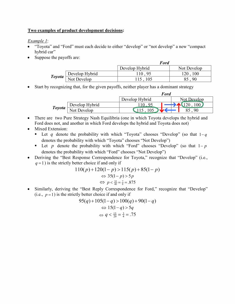
• Visually • The graph above illustrates all three equilibria of this game:
i. Pure Strategy Nash Equilibrium in which Toyota chooses “Develop” and Ford chooses “Not Develop” ( 1=q and 0=p )
ii. Pure Strategy Nash Equilibrium in which Toyota chooses “Not Develop” and Ford chooses “Develop” ( 0=q and 1=p )
iii. Mixed Strategy Nash Equilibrium in which Toyota chooses “Develop” with probability 75.=q and Ford chooses “Develop” with probability 875.=p
Example 2: (“cat and mouse game”) • Suppose Lexus and Hyundai must choose a design for their 2011 model, either “sleek” or
“boxy” • Hyundai wants their car to “look like the Lexus,” while Lexus wants their car to “look
different than the Hyundai”
Hyundai Sleek Hyundai Boxy Hyundai
Lexus Sleek Lexus 160 , 140 200 , 90 Boxy Lexus 170 , 110 130 , 120
• No Pure Strategy Nash Equilibrium => consider the Mixed Extension of the game Let q denote the probability with which “Hyundai” chooses “Sleek” (so that q−1
denotes the probability with which “Hyundai” chooses “Boxy”) Let p denote the probability with which “Lexus” chooses “Sleek” (so that p−1 denotes
the probability with which “Lexus” chooses “Boxy”) • Deriving the “Best Response Correspondence for Hyundai,” recognize that “Sleek” (i.e.,
1=q ) is the strictly better choice if and only if )1(120)(90)1(110)(140 pppp −+>−+
⇔ )1(1050 pp −>
⇔ 61.61
6010 ==>p
q
0
0 p
)(qBRF
1
.75
1
)( pBRT
.875
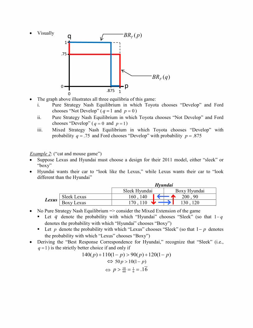
• Similarly, deriving the “Best Reply Correspondence for Lexus,” recognize that “Sleek” (i.e., 1=p ) is the strictly better choice if and only if
)1(130)(170)1(200)(160 qqqq −+>−+ ⇔ qq 10)1(70 >−
⇔ 875.87
8070 ==<q
• Visually • The graph above illustrates the unique equilibrium of this game => a Mixed Strategy Nash
Equilibrium in which Hyundai chooses “Sleek” with probability 87=q and Lexus chooses
“Sleek” with probability 61=p
q
0
0 p
)(qBRL
1
.875
1
)( pBRH
61
Basic Bertrand Model: • Market demand of )( pD • Two firms selling identical products => consumers base their purchasing decisions
simply upon price If firms set different prices, then all consumers will buy from the “lower price” firm If firms set the same price, they “split the market evenly” and each sell )(2
1 pDq = • Suppose the firms each have constant marginal costs of 11 cMC = and 22 cMC = (and
no Fixed Costs of production)
Basic Bertrand Model with Identical Costs… • Suppose 021 >== ccc • Recognize that neither firm would ever want to charge a price below c (since doing so only
ever leads to a negative profit or profit of zero) • If Firm 2 were to choose a price of 2p (with cp >2 ), what is the “best reply” of Firm 1?
21 pp > (charge a higher price than Firm 2) => 01 =q => 01 =π 21 pp = (charge the same price as Firm 2) => )( 22
11 pDq = =>
( ) 0)( 221
21 >−= pDcpπ ε−= 21 pp (slightly undercut the price of Firm 2) => )( 21 ε−= pDq =>
( ) 0)( 221 >−−−= εεπ pDcp • For “ε small enough,” ( ) ( ) )()( 22
1222 pDcppDcp −>−−− εε
• Thus, when Firm 2 charges a price of cp >2 , the Best Reply of Firm 1 is to choose ε−= 21 pp (i.e., slightly undercut the price of Firm 2 in order to get the entire market)
• But, when both firms behave in this way, the only stable pair of prices is cp =*1 and cp =*
2 => “Marginal Cost Pricing”
• When firms choose these prices… Each firm sells )(2
1 cD units and earns zero profit There is zero Deadweight-Loss (all units for which Buyer’s Reservation Price is greater
than Marginal Costs are produced) “two firms is enough for competition”
Basic Bertrand Model with Different Costs… • Suppose 210 cc << • Much of the same logic used for the case of “identical costs” can be applied • Doing so, it is clear that there can never be an equilibrium in which Firm 2 (the “higher cost
firm”) sells any positive quantity, since at such any outcome, Firm 1 could do better by slightly undercutting the price of Firm 2
• Thus, in equilibrium… Firm 2 will set a price equal to marginal costs ( 22 cp = ) Firm 1 will set a price below the marginal costs of Firm 2 and capture the entire market But, regarding the optimal choice of Firm 1, we have one of two possible cases,
depending upon whether there is a “slight difference” or a “big difference” in costs…
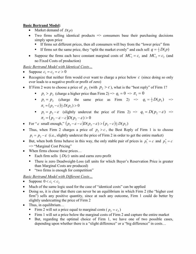
• If there is only a “slight difference in costs,” then Firm 1 will charge εε −=−= 221 cpp (i.e., slightly undercut Firm 2, but not move any further down the market demand curve) and sell )( 21 ε−= cDq units => visually (with linear demand)
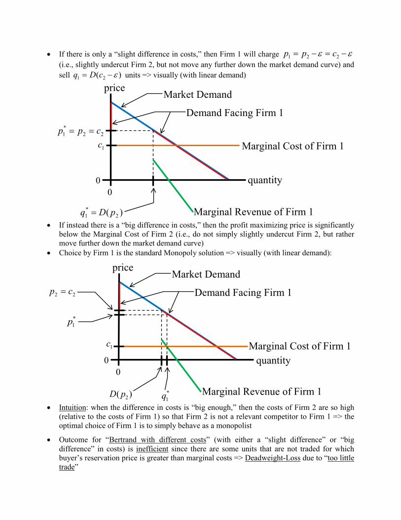
• If instead there is a “big difference in costs,” then the profit maximizing price is significantly below the Marginal Cost of Firm 2 (i.e., do not simply slightly undercut Firm 2, but rather move further down the market demand curve)
• Choice by Firm 1 is the standard Monopoly solution => visually (with linear demand):
22 cp = • Intuition: when the difference in costs is “big enough,” then the costs of Firm 2 are so high
(relative to the costs of Firm 1) so that Firm 2 is not a relevant competitor to Firm 1 => the optimal choice of Firm 1 is to simply behave as a monopolist
• Outcome for “Bertrand with different costs” (with either a “slight difference” or “big difference” in costs) is inefficient since there are some units that are not traded for which buyer’s reservation price is greater than marginal costs => Deadweight-Loss due to “too little trade”
price
0 0
quantity
Market Demand
22*1 cpp ==
Demand Facing Firm 1
)( 2*1 pDq = Marginal Revenue of Firm 1
1c Marginal Cost of Firm 1
price
0 0
quantity
Market Demand
Demand Facing Firm 1
)( 2pD Marginal Revenue of Firm 1
1c Marginal Cost of Firm 1
*1q
*1p
Bertrand Model with differentiated products: • Critical assumption of the basic Bertrand model: all consumers will purchase the product
from the firm charging the lower price (implicitly assumes that consumers view the products as identical to each other)
• If instead the products are differentiated from one another, then “Firm 1 can charge a slightly higher price than Firm 2 and still retain some customers…”
• But, if the two goods are substitutes for each other, then Firm 1 should expect to lose some customers as Firm 2 lowers its price (and vice versa)
• Example: Coke versus Pepsi => Gasmi, Vuong, and Laffont, “Econometric Analysis of Collusive Behavior in a Soft-Drink Market,” Journal of Economics and Management Strategy (Summer 1992): 277-311. Used sophisticated econometric techniques to estimate production costs and residual
demand for Coke and Pepsi for the period from 1968 through 1986 All prices are inflation adjusted and expressed in dollars per unit (a unit is 10 cases, with
twelve 24-ounce cans in each case), while quantities are expressed in millions of units of cola
Rounding the estimated values to the nearest integers… Residual demands of:
• PepsiCokeCoke ppq 2464 +−= for Coke
• CokePepsiPepsi ppq +−= 550 for Pepsi Marginal Costs of Production of:
• 5=CokeMC for Coke • 4=PepsiMC for Pepsi
If the firms compete by simultaneously choosing prices, what prices should they choose? Start by analyzing the problem from the perspective of Coke…
• Profit can be expressed as CokeCokeCokeCokeCokeCoke FqMCqp −−=π
( )( ) CokePepsiCokeCokeCokeCoke FppMCp −+−−= 2464π
( )( ) CokePepsiCokeCokeCoke Fppp −+−−= 24645π • Coke has direct control over its own price, but not over Pepsi’s price • Conceptually think about Coke identifying the value of Cokep to maximize Cokeπ , for any
arbitrary value of Pepsip => this derivation would give us ‘Coke’s Best Reply Function’
• Partial differentiation of Cokeπ with respect to Cokep yields
( )( )452464 −−++−=∂∂
CokePepsiCokeCoke
Coke ppppπ
2042464 +−+−= CokePepsiCoke ppp
CokePepsi pp 8284 −+=
(“Bertrand Model with differentiated products” continued)
• In order to maximize profit, Coke would want to operate where this expression is equal to zero
0=∂∂
Coke
Coke
pπ
⇔ 08284 =−+ CokePepsi pp
⇔ PepsiCoke pp 2848 +=
⇔ PepsiPepsiCoke ppp 41
221
82
884 +=+=
⇔ ( ) PepsiPepsiBRCoke ppp 4
1221 +=
• This final expression is “Coke’s Best Reply Function,” which specifies the optimal choice of price by Coke as a function of the price chosen by Pepsi
Similarly, for Pepsi…
• Profit can be expressed as ( )( ) PepsiCokePepsiPepsiPepsi Fppp −+−−= 5504π
• Conceptually think about Pepsi identifying the value of Pepsip to maximize Pepsiπ , for
any arbitrary value of Cokep => this derivation would give us ‘Pepsi’s Best Reply Function’
• Partial differentiation of Pepsiπ with respect to Pepsip yields
( )( )54550 −−++−=∂∂
PepsiCokePepsiPepsi
Pepsi ppppπ
PepsiCoke pp 1070 −+= • In order to maximize profit, Pepsi would want to operate where this expression is equal to
zero
0=∂∂
Pepsi
Pepsi
pπ
⇔ 01070 =−+ PepsiCoke pp
⇔ CokePepsi pp += 7010
⇔ CokeCokePepsi ppp 101
101
1070 7 +=+=
⇔ ( ) CokeCokeBRPepsi ppp 10
17 += • This final expression is “Pepsi’s Best Reply Function,” which specifies the optimal
choice of price by Pepsi as a function of the price chosen by Coke
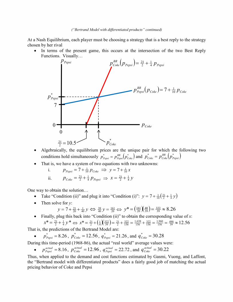
(“Bertrand Model with differentiated products” continued) At a Nash Equilibrium, each player must be choosing a strategy that is a best reply to the strategy chosen by her rival
• In terms of the present game, this occurs at the intersection of the two Best Reply Functions. Visually…
• Algebraically, the equilibrium prices are the unique pair for which the following two conditions hold simultaneously ( )**
CokeBRPepsiPepsi ppp = and ( )**
PepsiBRCokeCoke ppp =
• That is, we have a system of two equations with two unknowns: i. CokePepsi pp 10
17 += ⇒ xy 1017 +=
ii. PepsiCoke pp 41
221 += ⇒ yx 4
1221 +=
One way to obtain the solution…
• Take “Condition (ii)” and plug it into “Condition (i)”: ( )yy 41
221
1017 ++=
• Then solve for y: yy 40
120217 ++= ⇔ 20
1614039 =y ⇔ ( )( ) 26.8* 39
3223940
20161 ≈==y
• Finally, plug this back into “Condition (ii)” to obtain the corresponding value of x: ** 4
1221 yx += ⇔ ( )( ) 56.12* 39
490156960,1
156322
156638,1
156322
221
39322
41
221 ≈==+=+=+=x
That is, the predictions of the Bertrand Model are: • 26.8* =Pepsip , 56.12* =Cokep , 26.21* =Pepsiq , and 28.30* =Cokeq
During this time-period (1968-86), the actual “real world” average values were: • 16.8=actual
Pepsip , 96.12=actualCokep , 72.22=actual
Pepsiq , and 22.30=actualCokeq
Thus, when applied to the demand and cost functions estimated by Gasmi, Vuong, and Laffont, the “Bertrand model with differentiated products” does a fairly good job of matching the actual pricing behavior of Coke and Pepsi
0 0
*Pepsip
Pepsip
7
Cokep
( ) CokeCokeBRPepsi ppp 10
17 +=
( ) PepsiPepsiBRCoke ppp 4
1221 +=
5.10221 = *
Cokep

Cournot Model: • Market demand summarized by the inverse function )(QPD • Two firms simultaneously choose quantities of Aq and Bq => market quantity supplied
of BA qqQ += results in a price of )(QPD As an example, consider:
• QQPD −=100)( • Suppose the firms each have constant marginal costs of AA cMC = and BB cMC = (and
no Fixed Costs of production) • Under these assumptions, firm profits are
( ) ( ) AABAAADAAADA qcqqqcQPqcqQP −−−=−=−= 100)()(π and
( ) ( ) BBBABBDBBBDB qcqqqcQPqcqQP −−−=−=−= 100)()(π • Firm A gets to choose Aq , but not Bq • Start by deriving the “Best Reply Function” for Firm A
• Partial differentiation of Aπ with respect to Aq yields ( ) AABA
A qcqq
2100 −−−=∂∂π
• Setting this equal to zero and solving for Aq : 0=∂∂
A
A
qπ ⇔ ( ) 02100 =−−− AAB qcq
⇔ ( )ABA cqq −−= 1002 ⇔2
100 ABA
cqq −−=
⇔2
100)( ABB
BRA
cqqq −−=
• Similarly, for Firm B we would have (by symmetry) 2
100)( BAA
BRB
cqqq −−=
• Equilibrium of this simultaneous move game is the unique pair of quantities for which )( **
BBRAA qqq = and )( **
ABRBB qqq =
• Graphically:
0 0
*Bq
Bq
Aq
2100)( BA
ABRB
cqqq −−=
2100)( AB
BBRA
cqqq −−=
2100 Bc−
*Aq 2
100 Ac−
Bc−100
Ac−100

(“Cournot Model” continued)
• Algebraically, we again have a system of two equations with two unknowns:
(i) BA
A qcq21
2100
−−
= and (ii) AB
B qcq21
2100
−−
=
• Plugging Equation (ii) into Equation (i) and solving for Aq
−
−−
−= A
BAA qccq
21
2100
21
2100
⇔ ABA
A qccq41
4100
2100
+−
−−
=
⇔4
1004
220043 BA
Accq −
−−
=
⇔3
2100* ABA
ccq −+=
• Similarly, for Firm B we would obtain 3
2100* BAB
ccq −+=
• Total industry output is 3
200* ** BABB
ccqqQ −−=+=
• Thus, price is:
3100
3200100*)(* BABA
DccccQPP ++
=−−
−==
• Firm profits are:
( )
−+
−
++=−=
32100
3100* ** AB
ABA
AAAcccccqcPπ
2
32100
32100
32100
−+
=
−+
−+
= ABABAB cccccc
and
( )
−+
−
++=−=
32100
3100* ** BA
BBA
BBBcccccqcPπ
2
32100
32100
32100
−+
=
−+
−+
= BABABA cccccc
• From here we can easily obtain the intuitive results that an increase in Ac would result in:
o a decrease in *Aq , *Q , and *
Aπ
o an increase in *Bq , *P , and *
Bπ an increase in Bc would result in:
o a decrease in *Bq , *Q , and *
Bπ
o an increase in *Aq , *P , and *
Aπ

Multiple Choice Questions: 1. In the Cournot Model of competition, firms compete by A. sequentially choosing quantities of output. B. simultaneously choosing quantities of output. C. sequentially choosing prices. D. simultaneously choosing prices. 2. Consider a market in which ‘Firm A’ and ‘Firm B’ compete by simultaneously choosing
quantities of output ( Aq and Bq respectively). The ‘Best Reply Function for Firm A’ is
BBBRA qqq 2
140)( −= , and the ‘Best Reply Function for Firm B’ is AABRB qqq 2
135)( −= . It follows that at the Nash Equilibrium, Firm A will produce _____ units of output and Firm B will produce _____ units of output.
A. 30; 20. B. 40; 0. C. 40; 35. D. 80; 70. For questions 3 and 4, consider the following scenario. Firms A and B operate in a market with demand of ppD 900000,18)( −= . They compete by simultaneously setting prices. Consumers make no distinction between the output of Firm A and the output of Firm B (and will therefore simply buy from the firm offering the lower price). Firm A has production costs of qcqC AA =)( , and Firm B has production costs of qcqC BB =)( . 3. If 2== BA cc , then in equilibrium A. each firm will set a price of $11. B. there will be a positive Deadweight-Loss, due to “not enough trade.” C. each firm will earn zero profit. D. More than one (perhaps all) of the above answers is correct. 4. If 2=Ac and 1=Bc , then in equilibrium
A. both firms will sell a positive amount of output. B. both firms will earn a strictly positive profit. C. Deadweight-Loss will be equal to zero. D. None of the above answers are correct.
Problem Solving or Short Answer Questions: 1. Consider a market in which Firm A and Firm B compete by simultaneously choosing
quantities of output (denoted Aq and Bq respectively). Market demand is given by the inverse function QQPD 200
120)( −= , where BA qqQ += . Firm A has costs of 000,2)( += AAAA qcqC , while Firm B has costs of 500,1)( += BBBB qcqC .
1A. Derive and graphically illustrate the Best Reply Function of each firm. 1B. Suppose 7=Ac for the remainder of the question. Still allowing Bc to take on
any arbitrary value, determine expressions for the optimal quantity of Firm A and of Firm B (each as a function of Bc ). Clearly explain how the optimal level of output of each firm depends upon the value of Bc .
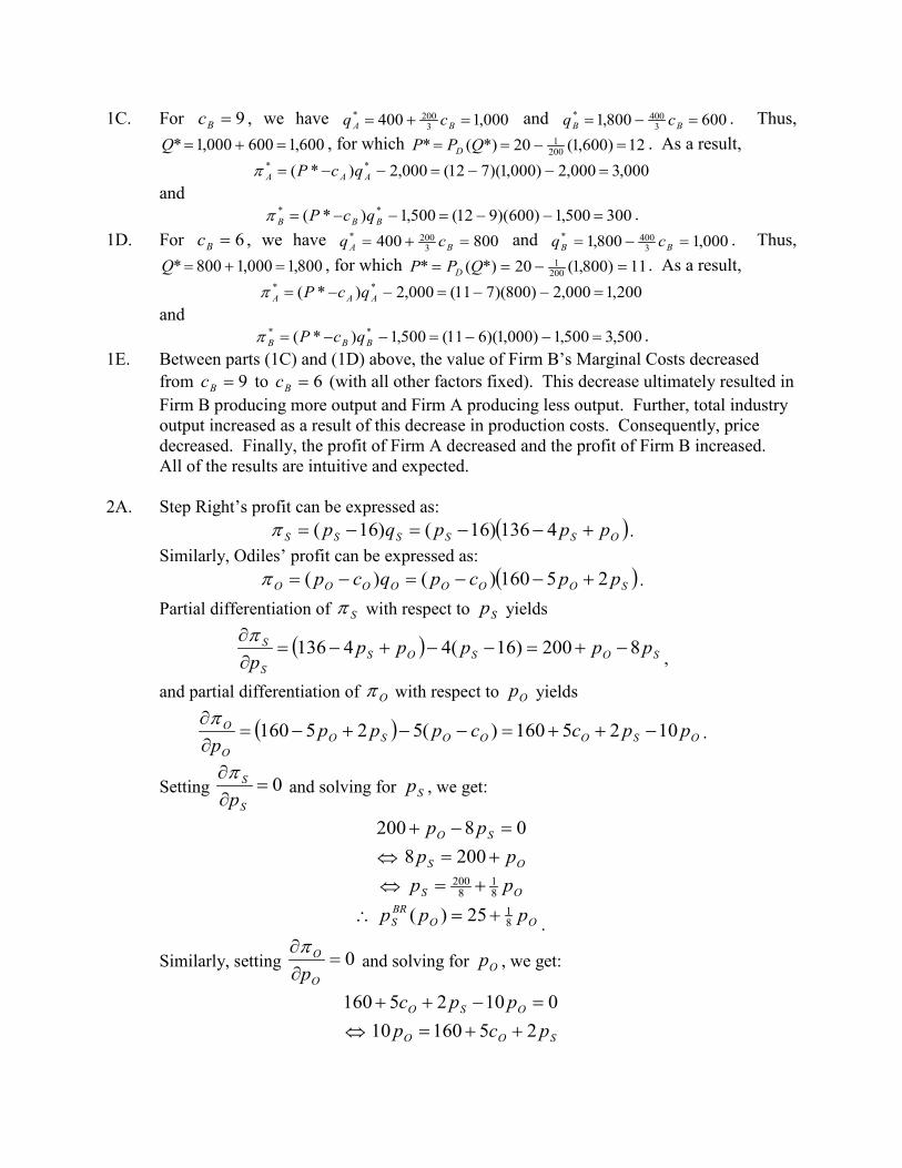
1C. Suppose 9=Bc . Determine the optimal level of output of each firm, along with the resulting market quantity of output, market price, and profit of each firm.
1D. Suppose 6=Bc . Determine the optimal level of output of each firm, along with the resulting market quantity of output, market price, and profit of each firm.
1E. Based upon your answers above, clearly explain how the optimal level of output of each firm, market quantity of output, market price, and profit of each firm each changed as the marginal costs of Firm B decreased from 9=Bc to 6=Bc .
2. “Step Right” and “Odiles” compete with each other in the market for children’s footwear
by simultaneously choosing prices. Residual demand for Step Right’s shoes is given by OSS ppq +−= 4136 , and residual demand for Odiles’ shoes is given by
SOO ppq 25160 +−= . Step Right has costs of SSS qqC 16)( = , and Odiles has costs
of OOOO qcqC =)( . Assume throughout that 21.440 19840 ≈<< Oc .
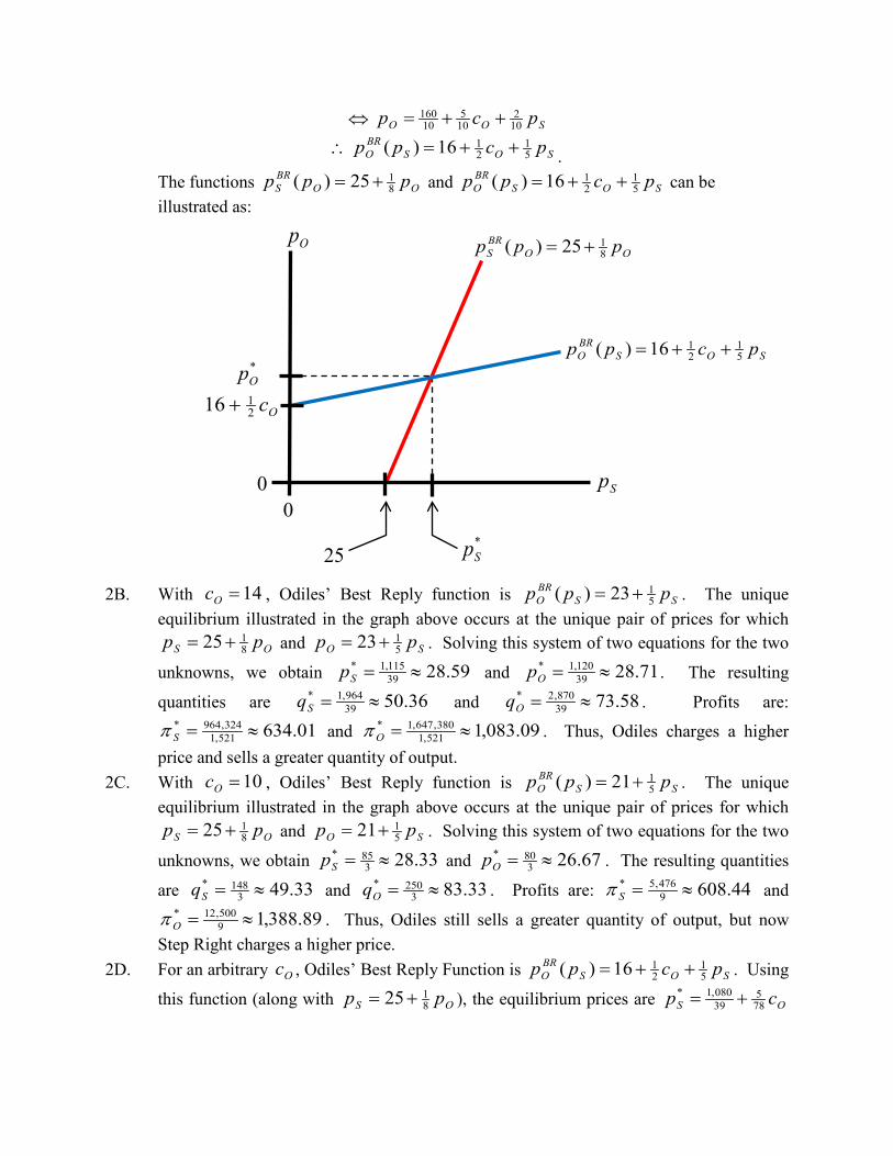
2A. Derive and graphically illustrate the Best Reply Functions for both Step Right and Odiles.
2B. Suppose 14=Oc . Determine the equilibrium price that each firm will set. Determine the corresponding quantity sold and profit for each firm. Which firm charges a higher price? Which firm sells a greater quantity of output?
2C. Suppose 10=Oc . Determine the equilibrium price that each firm will set. Determine the corresponding quantity sold and profit for each firm. Which firm charges a higher price? Which firm sells a greater quantity of output?
2D. Allowing Oc to take on any arbitrary value, determine the optimal price of each firm as a function of Oc . Determine the corresponding quantity sold and profit of each firm (again as functions of Oc ).
2E. Explain how each of the functions in part (2D) behaves as the value of Oc is increased.
2F. Determine the range of Oc for which Odiles sets a higher price than Step Right. 2G. Determine the range of Oc for which Odiles sells more output than Step Right.
3. Consider a market in which Firm A and Firm B compete by simultaneously choosing prices. Consumers make no distinction between the output of Firm A and the output of Firm B (and therefore base their purchasing decision upon only price). Market Demand is given by ppD 320000,16)( −= . Firm A has production costs of qqC A 28)( = , while Firm B has production costs of qcqC BB =)( . Assume throughout that 28≤Bc . 3A. Suppose 28=Bc . Determine the equilibrium price of each firm. Determine the
resulting quantity sold by each firm, profit of each firm, and Deadweight-Loss in this market.
3B. Suppose 24=Bc . Determine the equilibrium price of each firm. Determine the resulting quantity sold by each firm, profit of each firm, and Deadweight-Loss in this market.
3C. Will Firm B ever want to undercut the price of Firm A by “more than ε ”? If so, determine the range of Bc for which Firm B would want to do so.
4. “Golden Fleece” and “JonShawn” are two firms that produce men’s clothing. They must
simultaneously choose their product lines for next year. They each broadly have a choice of either a “traditional line” or a “trendy line.” Historically, the clothing of Golden Fleece has tended to appeal to consumers with conservative tastes, while the clothing of JonShawn has tended to appeal to those consumers who want to be on the cutting edge of fashion. If the two firms choose similar lines, then their products will be less differentiated from one another. As a result, they would be competing for essentially the same segment of consumers, making joint profits lower. More precisely, the profits of the firms will be: 95=GFπ and 70=JSπ , if both introduce a “traditional line”; 85=GFπ and 120=JSπ , if both introduce a “trendy line”; 155=GFπ and 200=JSπ , if Golden Fleece introduces a “Trendy line” and JonShawn introduces a “traditional line”; and
185=GFπ and 220=JSπ , if Golden Fleece introduces a “traditional line” and JonShawn introduces a “trendy line.”
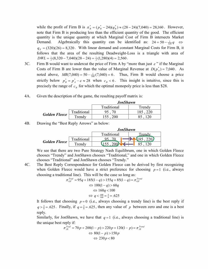
4A. Illustrate the interaction between these two firms by way of a payoff matrix. 4B. Identify all Pure Strategy Nash Equilibria of this game.
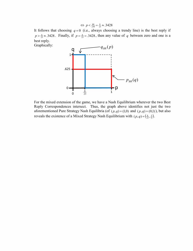
4C. Considering the Mixed Extension of the game (in which Golden Fleece chooses “traditional line” with probability p and JonShawn chooses “traditional line” with probability q ), graphically illustrate the Best Reply Correspondence of each player. Based upon this graph, identify any Mixed Strategy Nash Equilibria of this game.
Answers to Multiple Choice Questions:
1. B 2. A 3. C 4. D
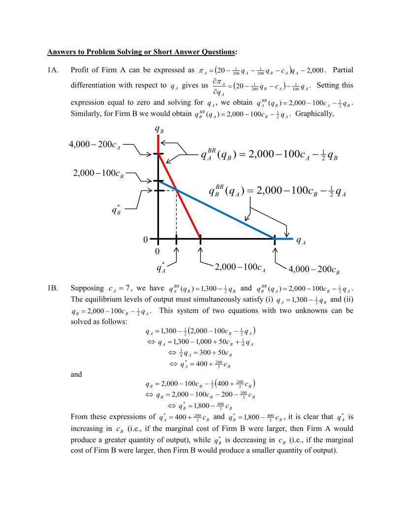
Answers to Problem Solving or Short Answer Questions: 1A. Profit of Firm A can be expressed as ( ) 000,220 200
12001 −−−−= AABAA qcqqπ . Partial
differentiation with respect to Aq gives us ( ) AABA
A qcqq 100
1200120 −−−=
∂∂π . Setting this
expression equal to zero and solving for Aq , we obtain BABBRA qcqq 2
1100000,2)( −−= . Similarly, for Firm B we would obtain ABA
BRB qcqq 2
1100000,2)( −−= . Graphically, 1B. Supposing 7=Ac , we have BB
BRA qqq 2
1300,1)( −= and ABABRB qcqq 2
1100000,2)( −−= . The equilibrium levels of output must simultaneously satisfy (i) BA qq 2
1300,1 −= and (ii)
ABB qcq 21100000,2 −−= . This system of two equations with two unknowns can be
solved as follows: ( )ABA qcq 2
121 100000,2300,1 −−−=
⇔ ABA qcq 4150000,1300,1 ++−=
⇔ BA cq 5030043 +=
⇔ BA cq 3200* 400 +=
and ( )BBB ccq 3
20021 400100000,2 +−−=
⇔ BBB ccq 3100200100000,2 −−−=
⇔ BB cq 3400* 800,1 −=
From these expressions of BA cq 3200* 400 += and BB cq 3
400* 800,1 −= , it is clear that *Aq is
increasing in Bc (i.e., if the marginal cost of Firm B were larger, then Firm A would produce a greater quantity of output), while *
Bq is decreasing in Bc (i.e., if the marginal cost of Firm B were larger, then Firm B would produce a smaller quantity of output).
0 0
*Bq
Bq
Aq
ABABRB qcqq 2
1100000,2)( −−=
BABBRA qcqq 2
1100000,2)( −−=
Bc100000,2 −
*Aq Ac100000,2 −
Bc200000,4 −
Ac200000,4 −
1C. For 9=Bc , we have 000,1400 3200* =+= BA cq and 600800,1 3
400* =−= BB cq . Thus, 600,1600000,1* =+=Q , for which 12)600,1(20*)(* 200
1 =−== QPP D . As a result, 000,3000,2)000,1)(712(000,2)*( ** =−−=−−= AAA qcPπ
and 300500,1)600)(912(500,1)*( ** =−−=−−= BBB qcPπ .
1D. For 6=Bc , we have 800400 3200* =+= BA cq and 000,1800,1 3
400* =−= BB cq . Thus, 800,1000,1800* =+=Q , for which 11)800,1(20*)(* 200
1 =−== QPP D . As a result, 200,1000,2)800)(711(000,2)*( ** =−−=−−= AAA qcPπ
and 500,3500,1)000,1)(611(500,1)*( ** =−−=−−= BBB qcPπ .
1E. Between parts (1C) and (1D) above, the value of Firm B’s Marginal Costs decreased from 9=Bc to 6=Bc (with all other factors fixed). This decrease ultimately resulted in Firm B producing more output and Firm A producing less output. Further, total industry output increased as a result of this decrease in production costs. Consequently, price decreased. Finally, the profit of Firm A decreased and the profit of Firm B increased. All of the results are intuitive and expected.
2A. Step Right’s profit can be expressed as:
( )OSSSSS pppqp +−−=−= 4136)16()16(π . Similarly, Odiles’ profit can be expressed as:
( )SOOOOOOO ppcpqcp 25160)()( +−−=−=π . Partial differentiation of Sπ with respect to Sp yields
( ) SOSOSS
S pppppp
8200)16(44136 −+=−−+−=∂∂π
,
and partial differentiation of Oπ with respect to Op yields
( ) OSOOOSOO
O ppccpppp
1025160)(525160 −++=−−+−=∂∂π
.
Setting 0=∂∂
S
S
pπ
and solving for Sp , we get:
08200 =−+ SO pp ⇔ OS pp += 2008 ⇔ OS pp 8
18
200 +=
∴ OOBRS ppp 8
125)( += .
Similarly, setting 0=∂∂
O
O
pπ
and solving for Op , we get:
01025160 =−++ OSO ppc ⇔ SOO pcp 2516010 ++=
⇔ SOO pcp 102
105
10160 ++=
∴ SOSBRO pcpp 5
12116)( ++= .
The functions OOBRS ppp 8
125)( += and SOSBRO pcpp 5
12116)( ++= can be
illustrated as: 2B. With 14=Oc , Odiles’ Best Reply function is SS
BRO ppp 5
123)( += . The unique equilibrium illustrated in the graph above occurs at the unique pair of prices for which
OS pp 8125+= and SO pp 5
123+= . Solving this system of two equations for the two
unknowns, we obtain 59.2839115,1* ≈=Sp and 71.2839
120,1* ≈=Op . The resulting
quantities are 36.5039964,1* ≈=Sq and 58.7339
870,2* ≈=Oq . Profits are: 01.634521,1
324,964* ≈=Sπ and 09.083,1521,1380,647,1* ≈=Oπ . Thus, Odiles charges a higher
price and sells a greater quantity of output. 2C. With 10=Oc , Odiles’ Best Reply function is SS
BRO ppp 5
121)( += . The unique equilibrium illustrated in the graph above occurs at the unique pair of prices for which
OS pp 8125+= and SO pp 5
121+= . Solving this system of two equations for the two
unknowns, we obtain 33.28385* ≈=Sp and 67.263
80* ≈=Op . The resulting quantities
are 33.493148* ≈=Sq and 33.833
250* ≈=Oq . Profits are: 44.6089476,5* ≈=Sπ and
89.388,19500,12* ≈=Oπ . Thus, Odiles still sells a greater quantity of output, but now
Step Right charges a higher price. 2D. For an arbitrary Oc , Odiles’ Best Reply Function is SOS
BRO pcpp 5
12116)( ++= . Using
this function (along with OS pp 8125+= ), the equilibrium prices are OS cp 78
539080,1* +=
0 0
*Op
Op
Oc2116 +
Sp
SOSBRO pcpp 5
12116)( ++=
OOBRS ppp 8
125)( +=
25 *Sp

and OO cp 3920
39840* += . The corresponding quantities of output are
3910824,1* O
Scq +
=
and 39
95200,4* OO
cq −= . The resulting profits are:
2*
395912
+
= OS
cπ and
2*
39198405
−
= OO
cπ .
2E. As Oc is increased, OS cp 785
39080,1* += and OO cp 39
2039
840* += both increase. Further,
3910824,1* O
Scq +
= increases, while 39
95200,4* OO
cq −= decreases. Finally,
2*
395912
+
= OS
cπ increases, while
2*
39198405
−
= OO
cπ decreases.
2F. OO cp 3920
39840* += is greater than OS cp 78
539080,1* += if and only if: 71.137
96 ≈>Oc .
2G. 39
95200,4* OO
cq −= is greater than
3910824,1* O
Scq +
= if and only if:
63.2235792 ≈<Oc .
3A. Throughout the question we are assuming 28=Ac (i.e., the Marginal Costs of Firm A are
a constant $28 per unit). If we additionally have 28=Bc , then the firms have identical costs. The only equilibrium when the firms choose prices simultaneously is for both firms to set price equal to $28 – that is, 28** == BA pp . At this price a total of
040,7)28)(320(000,16)28( =−=D units are sold, with the firms splitting the market evenly (i.e., each selling 3,520 units). This outcome is efficient, since all units for which Marginal Costs are below Buyer’s Reservation Price are indeed traded. Thus, Deadweight-Loss is equal to zero. Finally, each firm earns zero profit, since price is equal to the constant valued Marginal Costs of production (and Fixed Costs are zero).
3B. If instead 24=Bc , it is now the case that Firm B has strictly lower Marginal Costs than Firm A. In such instances, the equilibrium is such that Firm A will set 28* == AA cp , while Firm B will set price strictly below this level. For such prices, Firm A does not sell any output, while Firm B sells to all consumers who purchase the good. It is necessary to determine if Firm B wants to simply undercut the price of Firm A by an infinitesimal amount (i.e., charge a price of εε −=−= 28**
AB pp with 0≈ε ) or undercut the price of Firm B by a more substantial amount. To address this issue, it is helpful to graphically

illustrate market demand and the demand facing Firm B when Firm A sets 28* == AA cp . These functions can be illustrated as:
Recognize that with Market Demand of ppD 320000,16)( −= , Inverse Market Demand is QQPD 320
150)( −= . Thus, a firm serving the entire market (as Firm B would do if charging a price below $28) would have Marginal Revenue of QQMR 160
150)( −= . It follows that at a quantity of 7,040, 6)040,7(50)040,7( 160
1 =−=MR , as illustrated above. For 24=Bc , we have:
From the graph above, we can infer that the best choice by Firm B is 28** ≈−= εAB pp . That is, Firm B will “just slightly undercut” the price of Firm A. When 28* =Ap and
28** ≈−= εAB pp , it follows that Firm A does not sell any output and Firm B sells ( ) 040,7)28(28* =≈−= DDqB ε units of output. The profit of Firm A is clearly zero,
price
0 0
quantity
Market Demand (blue line)
28* == AA cp
Demand Facing Firm 1 (red line)
040,7)28()( * == DpD A Marginal Revenue of Firm 1 (green line)
24=Bc Marginal Cost of Firm B
(orange line)
50
25
000,16
000,8
6
price
0 0
quantity
Market Demand (blue line)
28* == AA cp
Demand Facing Firm B (red line)
040,7)28()( * == DpD A Marginal Revenue of Firm B (green line)
50
25
000,16
000,8
6
while the profit of Firm B is 160,28)040,7)(2428())(24( *** =−≈−= BBB qpπ . However, note that Firm B is producing less than the efficient quantity of the good. The efficient quantity is the unique quantity at which Marginal Cost of Firm B intersects Market Demand. Algebraically this quantity can be identified as: q320
15024 −= ⇔ 320,8)26)(320( ==Eq . With linear demand and constant Marginal Costs for Firm B, it
follows that the area of the resulting Deadweight-Loss is a triangle with area of 560,2)4)(280,1()2428)(040,7320,8( 2
121 ==−−=DWL .
3C. Firm B would want to undercut the price of Firm A by “more than just ε ” if the Marginal Costs of Firm B are lower than the value of Marginal Revenue at 040,7)( * =ApD . As noted above, 6)040,7(50)040,7( 160
1 =−=MR . Thus, Firm B would choose a price strictly below 28** ≈−= εAB pp when 6<Bc . This insight is intuitive, since this is precisely the range of Bc for which the optimal monopoly price is less than $28.
4A. Given the description of the game, the resulting payoff matrix is:
JonShawn Traditional Trendy
Golden Fleece Traditional 95 , 70 185 , 220 Trendy 155 , 200 85 , 120
4B. Drawing the “Best Reply Arrows” as below:
JonShawn Traditional Trendy
Golden Fleece Traditional 95 , 70 185 , 220 Trendy 155 , 200 85 , 120
We see that there are two Pure Strategy Nash Equilibrum, one in which Golden Fleece chooses “Trendy” and JonShawn chooses “Traditional,” and one in which Golden Fleece chooses “Traditional” and JonShawn chooses “Trendy.”
4C. The Best Reply Correspondence for Golden Fleece can be derived by first recognizing when Golden Fleece would have a strict preference for choosing 1=p (i.e., always choosing a traditional line). This will be the case so long as:
TrendGF
TradGF qqqq ππ =−+>−+= )1(85155)1(18595
⇔ qq 60)1(100 >− ⇔ 100160 <q
⇔ 625.85
160100 ==<q
It follows that choosing 0=p (i.e., always choosing a trendy line) is the best reply if 625.8
5 =>q . Finally, if 625.85 ==q , then any value of p between zero and one is a best
reply. Similarly, for JonShawn, we have that 1=q (i.e., always choosing a traditional line) is
the unique best reply if: TrendJS
TradJS pppp ππ =−+>−+= )1(120220)1(20070
⇔ pp 150)1(80 >− ⇔ 80230 <p
⇔ 3428.238
23080 ≈=<p
It follows that choosing 0=q (i.e., always choosing a trendy line) is the best reply if 3428.23
8 ≈>p . Finally, if 3428.238 ==p , then any value of q between zero and one is a
best reply. Graphically:
For the mixed extension of the game, we have a Nash Equilibrium wherever the two Best Reply Correspondences intersect. Thus, the graph above identifies not just the two aforementioned Pure Strategy Nash Equilibria (of )0,1(),( =qp and )1,0(),( =qp ), but also reveals the existence of a Mixed Strategy Nash Equilibrium with ( )8
5238 ,),( =qp .
q
0
0 p
)(qpBR
1
.625
1
)( pqBR
238
Top Related