


Languages
Pages
Legal


Retrospective Theses and Dissertations Iowa State University Capstones, Theses andDissertations
1965
Dynamic testing in the control of a pulse columnDennis Rex EvansIowa State University
Follow this and additional works at: https://lib.dr.iastate.edu/rtd
Part of the Chemical Engineering Commons
This Dissertation is brought to you for free and open access by the Iowa State University Capstones, Theses and Dissertations at Iowa State UniversityDigital Repository. It has been accepted for inclusion in Retrospective Theses and Dissertations by an authorized administrator of Iowa State UniversityDigital Repository. For more information, please contact [email protected].
Recommended CitationEvans, Dennis Rex, "Dynamic testing in the control of a pulse column " (1965). Retrospective Theses and Dissertations. 4083.https://lib.dr.iastate.edu/rtd/4083
This dissertation has been
microfihned exactly as received 66-2958
EVANS, Dennis Rex, 1937-DYNAMIC TESTING IN THE CONTROL OF A PULSE COLUMN.
Iowa State University of Science and Technology Ph.D., 1965 Engineering, chemical
University Microfilms, Inc., Ann Arbor, Michigan
DYNAMIC TESTING IN THE CONTROL OF A PULSE COLUMN
by
A Dissertation Submitted to the
Graduate Faculty in Partial Fulfillment of
The Requirements for the Degree of
DOCTOR OF PHILOSOPHY
Major Subject: Chemical Engineering
Dennis Rex Evans
Approved :
In Charge of Major Work
Head of Major Department
Iowa State University Of Science and Technology
Ames, Iowa
1965
Signature was redacted for privacy.
Signature was redacted for privacy.
Signature was redacted for privacy.

ii
TABLE OF CONTENTS
Page
ABSTRACT vii
INTRODUCTION 1
LITERATURE REVIEW 4
Pulse Column Dynamics and Control 4
Control Systems Analysis 10
Pulse Testing 12
THEORETICAL BACKGROUND 15
Dynamic Testing 15
Pulse Testing 16
Limitations of Pulse Testing 28
Validity of linearity assumption 28
Pulse testing compared to mathematical simulation 31
Pulse testing compared to sinusoidal forcing 32
EQUIPMENT 35
Characteristics of a Pulse Column 35
Experimental Pulse Column 36
PROCEDURE 40
Liquid-Liquid Extraction System 40
Operation of Column 40
RESULTS 43
DISCUSSION OF RESULTS 75
CONTROL ANALYSIS 82
CONCLUSIONS AND RECOMMENDATIONS 91

iii
Page
TABLE OF NOMENCLATURE 93a
English Letters 93a
Greek Letters 93b
Subscripts 93b
LITERATURE CITED 94
ACKNOWLEDGMENTS 96

iv
LIST OF FIGURES
Page
Figure 1. Response of pulse column to changes in operating variables 9
Figure 2. Differently shaped pulses 20
Figure 3. Typical output pulse to be transformed 23
Figure 4. Frequency content of pulses versus frequency 27
Figure 5. Liquid level process 30
Figure 6. Effect of size of change on accuracy of linearization 30
Figure 7. Schematic of pulse column 38
Figure 8. Calculated frequency response for Run 1. One hundred per cent decrease in aqueous feed concentration for 10 minutes 46
Figure 9. Calculated frequency response for Run 2. One hundred per cent increase in aqueous feed concentration for 10 minutes 48
Figure 10. Calculated frequency response for Run 3. One hundred per cent decrease in column pulse frequency for 5 minutes 50
Figure 11. Calculated frequency response for Run 4. Fifty per cent increase in column pulse frequency for 5 minutes 52
Figure 12. Calculated frequency response for Run 5. Fifty per cent decrease in aqueous phase flow rate for 5 minutes 55
Figure 13. Calculated frequency response for Run 6. Fifty per cent increase in aqueous phase flow rate for 5 minutes 57
Figure 14. Calculated frequency response for Run 7. Fifty per cent decrease in organic flow rate for 2 1/2 minutes 59
V
Page
Figure 15. Calculated frequency response for Run 8. Ten per cent increase in organic phase flow rate for 5 minutes 61
Figure 16. Calculated frequency response for Run 9. One hundred per cent decrease in aqueous feed concentration for 2 1/2 minutes 63
Figure 17. Calculated frequency response for Run 10. One hundred per cent increase in aqueous feed concentration for 5 minutes 65
Figure 18a. Comparison of simulations to time response for Run 5. Decrease in aqueous flow rate 70
Figure 18b. Comparison of simulations to time response for Run 6. Increase in aqueous phase flow rate 70
Figure 19a. Comparison of simulations to time response for Run 7. Decrease in organic phase flow rate 72
Figure 19b. Comparison of simulations to time response for Run 8. Increase in organic phase flow rate 72
Figure 20a. Comparison of simulations to time response for Run 9. Decrease in aqueous feed concentration 74
Figure 20b. Comparison of simulations to time response for Run 10. Increase in aqueous feed concentration 74
Figure 21. Block diagram for differential equations of pulse column 81
Figure 22. Block diagram for feedback control 84
Figure 23. Block diagram for feed-forward control 84
Figure 24. Block diagram for combined feedback and feedforward control 84
Figure 25. Analog computer diagram for simulating feedback control on pulse column 87
Figure 26a. Error-time curve in response to a step change in aqueous feed concentration 89
Figure 26b. Error-time curve in response to a step change in aqueous feed concentration 89

vi
LIST OF TABLES
Page
Table 1. Summary of models from pulse testing 67
vii
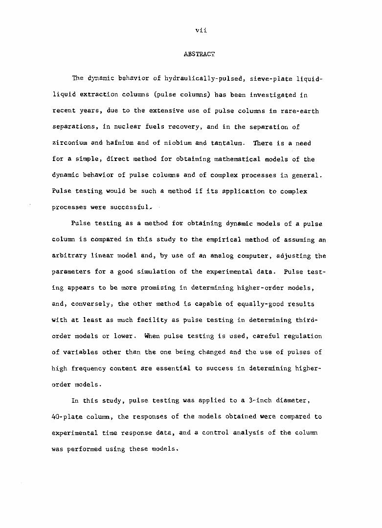
ABSTRACT
The dj'naisic behavior of hydraulically-pulsed, sieve-plate liquid-
liquid extraction columns (pulse columns) has been investigated in
recent years, due to the extensive use of pulse columns in rare-earth
separations, in nuclear fuels recovery, and in the separation of
zirconium and hafnium and of niobium and tantalum. There is a need
for a simple, direct method for obtaining mathematical models of the
dynamic behavior of pulse columns and of complex processes in general.
Pulse testing would be such a method if its application to complex
processes were successful^
Pulse testing as a method for obtaining dynamic models of a pulse
column is compared in this study to the empirical method of assuming an
arbitrary linear model and, by use of an analog computer, adjusting the
parameters for a good simulation of the experimental data. Pulse test
ing appears to be more promising in determining higher-order models,
and, conversely, the other method is capable of equally-good results
with at least as much facility as pulse testing in determining third-
order models or lower. When pulse testing is used, careful regulation
of variables other than the one being changed and the use of pulses of
high frequency content are essential to success in determining higher-
order models.
In this study, pulse testing was applied to a 3-inch diameter,
40-plate column, the responses of the models obtained were compared to
experimental time response data, and a control analysis of the column
was performed using these models.

viii
The pulse test results show that underdaraped second-order models
represent the calculated frequency responses of the raffinate concentra
tion to changes in column pulse frequency, aqueous phase flow rate, and
organic phase flow rate. Underdaraped second-order models including
transportation delay represent the calculated frequency responses to
changes in aqueous feed concentration. However, the more sensitive
comparison of experimental time response to simulated time response
showed less agreement than the frequency response comparisons. It was
found that excellent agreement of the simulations with initial portions
of the time response curves could be achieved by adjusting the natural
frequencies of the second-order models.
The results of the control analysis in this study are compared to
results of an earlier study, and qualitative agreement between the
results of both studies was achieved.

1
INTRODUCTION
The use of hydraulically-pulsed, sieve-plate liquid-liquid extraction
columns (pulse columns) is becoming widespread in rare-earth separations,
nuclear fuels recovery, and in the separation of zirconium and hafnium
and of niobium and tantalum. Common to all of these separations are
separation factors close to unity and rigid requirements of purity. As
is usually the case with complex operations, making pulse columns operable
has received more emphasis than has optimizing control. Although the
dynamics of pulse columns have been examined in recent years, much re
mains to be done.
The design and development of a control system for a pulse column is
complicated by the distributed nature and non-linear behavior of the
process. Di Liddo and Walsh (9) made a fundamental study of control for
a pulse column, but the possibilities for practical application of their
method are limited. There is a need for a direct, simple method of
deriving dynamic models for a pulse column for use in a control analysis.
Pulse testing*, as described by Dreifke and Hougen (12), is such a method.
Pulse testing could be used to determine dynamic models for a pulse column,
and these models could subsequently be used in making a control analysis
of the column. This testing method has not been applied to a pulse
column as large as the one used in this study. Such a pulse column
comprises a complex process, and success in the application of pulse
*The terms "pulse testing" and "pulse column" should not be confused, since "pulse" in the case of a pulse column refers to the motion of the continuous phase, while "pulse" in pulse testing refers to the type of disturbing function applied to the input of the system being tested.

2
testing to a pulse column suggests that similarly complex processes would
be amenable to pulse testing. Thus, if successful when applied to a pulse
column, pulse testing would appear to be a generally applicable method
in analyzing complex processes, as well as simple ones. Therefore, one
purpose of this study is the determination of the applicability of pulse
testing to complex processes, as well as the determination of operational
factors essential to successful use, but not obvious from theory.
Basic to a control analysis is the determination of the controlled
variable and of the control variable (manipulated to make desired changes
in the controlled variable). The controlled variable must be a dependent
variable, either the extract acid concentration or the raffinate acid
concentration. The control variable would be one of the independent
variables of the pulse column, which are:
1. Pulse stroke length
2. Pulse frequency
3. Aqueous phase flow rate
4. Organic phase flow rate
5. Aqueous feed concentration
6. Organic feed concentration
Having determined the controlled variable and the control variable,
it is necessary to determine mathematical models relating changes in
the controlled variable to changes in the control variable (process) and
those which relate changes in the controlled variable to changes in other
independent variables subject to perturbations during operation of the
column (loads). A control analysis may be made with the mathematical
models for the process and for the loads using an analog computer to

3
ascertain stability and controllability over a range of reset rate,
proportional band, and derivative time.
The purposes of this study are to evaluate the applicability of
pulse testing to the determination of dynamic models for a pulse column
and to perform a control analysis in which the appropriate control vari
ables and the type of control required are determined.
4
LITERATURE REVIEW
Pulse Column Dynamics and Control
Biery (2) presents an extensive survey of the literature on dynamics
of two-phase contacters from the earliest reports of such work. His
survey is especially valuable in ascertaining the status of work on the
dynamics of two-phase contacters. Notable is the recurrence in a large
number of studies of the following equations in one form or another:
^ It " I? " (1)
„ ôy By ôt âz KGa(y*-y) (2)
Where
h = Heavy phase holdup, pounds/foot
H = Light phase holdup, pounds/foot
X = Concentration in heavy phase, dimensionless
y = Concentration in light phase, dimensionless
L = Flow rate of heavy phase, pounds/hour
V = Flow rate of light phase, pounds/hour
Kga = Mass transfer coefficient for interphase transfer, pounds/(hour)(foot)
y* = Concentration in the light phase which would be in equilibrium with a concentration x in the heavy phase, dimensionless
t = Time, hours
z = Distance through column, feet.
Experience has shown that these equations will hold reasonably well
for many countercurrent two-phase contacters, as long as the appropriate
5
boundary conditions are specified and accurate solution techniques are
used.
Inherent in the derivation of Equations 1 and 2 are the following
assumptions :
1. No longitudinal mass diffusion takes place.
2. The interphase mass transport may be expressed by the empirical
relation Kga(y*-y), which is defined for steady state, and may
or may not hold under unsteady state conditions.
3. The holdups H and h are not functions of time.
Various solution and linearization techniques may be applied to Equations
I and 2; numerical integration on a digital computer with interpolation
of stored equilibrium data, such as was done by Biery, seems to give
reasonable approximations to transient response data taken on a pulse
column.
Biery solved Equations 1 and 2 by assuming a number of models of the
system to apply, with all models having in common the division of the
column into discrete stages without regard to the sieve plates in the
column. Inherent in his Model I was the assumption of the phases in each
stage to be perfectly mixed and at equilibrium. The assumptions of Model
II were that the phases were perfectly mixed but not at equilibrium.
Models III, IV, and V were similar to each other in the assumption that
the phases were neither perfectly mixed nor at equilibrium and were differ
ent from each other in how the concentrations for calculating the inter
phase mass transport were obtained. In the case of Model III the concen
trations of each phase were taken as the average of those at the top and
bottom of the stage. In the cases of Models IV and V, the concentrations

6
of each phase were taken at the bottom and at the top of the stage,
respectively. Model VI was an attempt to combine the good points of
Models IV and V. Models VII, VIII, and IX involved the use of a finite
difference representation of the differential equations. Biery reports
that Models IV and V were the most extensively used due to the rapid
convergence of the calculated solutions to the experimental data as the
number of stages was increased.
Di Liddo and Walsh (9) used a digital computer to simulate a pulse
column extracting nitric acid and uranyl nitrate between water and tributyl
phosphate-kerosene. Their simulation technique embodied the following
steps:
1. The pulse column is divided into a number of stages in series;
these stages are the upper and lower disengagement sections and
the spaces between successive sieve plates in the column.
2. After each half-cycle of the pulsing mechanism, material balance
and mass transport relations are solved and the new solute
concentrations of both phases in the stage are calculated.
3. A set of controller equations is solved to adjusc the aqueous
feed rate after each full cycle of the pulsing mechanism.
Three types of equations were used in the simulation:
1. Hydrodynamic equations for describing the flow of the phases in
the column and for predicting flooding.
2. Material balance and mass transport relations for calculating
the solute rate of accumulation.
3. The equations of the controller for describing the changes
in the aqueous feed rate.
Using the above equations the following studies were carried out assuming

7
a 3-stage column having extraction efficiencies of 100% and a 9-stage
column having experimentally-determined extraction efficiencies:
1. Studies to show the response of the column to changes in the
concentration of feed streams from zero concentration.
2. Studies to determine effects of changes from steady operating
conditions of the operating variables pulse frequency, organic
phase flow rate, and the organic feed concentration on the con
centration in the extract leaving the uncontrolled column.
3. Studies to determine the effectiveness of feedback integral
and proportional control in maintaining a steady operating
level of the extract concentration after various operating
variables were step-changed.
The results of the start up studies were similar to Biery's results, thus
demonstrating that quite different simulation techniques can be used to
describe the same class of equipment with comparable results.
The effects of operating variables on the uncontrolled raffinate
concentration differ quite markedly from each other for the same percentage
change, as may be seen from Figure 1. It may be seen that there is a
dramatic overall response to changes in the organic feed concentration or
flow rate, but that, although the overall response is smaller, the change
in pulse frequency causes a more rapid response. The rapidity indicates
the presence of fewer lags for changes in pulse frequency and encourages
the possibility of using the pulse frequency as a control variable.
The effectiveness of the controller in maintaining control of the sys
tem was hampered by the possibility of flooding when compensating for 25
per cent changes. However, as may be expected, the controller is capable

Figure 1. Response of pulse column to changes in operating variables
LLI
25% INCREASE IN ORGANIC FLOW RATE
2 5 % I N C R E A S E I N O R G A N I C FEED CONCENTRATION 0.8
<0.7 25% INCREASE IN COLUMN PULSE FREQUENCY
w
0.6 OS O 1.0 IS
TIME, MINUTES
10
of maintaining reasonably level conditions when changes in the operating
variables are kept as small as 10 per cent.
Control Systems Analysis
A well-developed body of theory and methods for linear control system
analysis is available. (A linear control system is one describable by
linear ordinary differential equations with constant coefficients.) A
few basic results of linear analysis will be reported in the following
paragraphs. More complete information may be found in many excellent
texts on control system analysis (4, 6, 10, 16), of which those cited are
a small fraction.
In the case of a linear system, the transfer function = f(s),
where 9^ = Laplace-transformed output
9^ = Laplace-transformed input
s = Laplace variable
is independent of 0^; therefore the transfer function may be determined
from the response to any input. If the input is sinusoidal, the output
will be a sinusoid which differs from the input sinusoid only in phase
and amplitude.
The output has two types of response to a step change: oscillatory
and non-oscillatory. The oscillatory solution is, for most systems, a
product of a decaying exponential and a sinusoid (damped oscillation).
In addition, an oscillation may oscillate with no change in amplitude or
with increasing amplitude. The non-oscillatory solution is normally a
decaying exponential. The solution of a linear differential equation will
be a sum of oscillatory and non-oscillatory responses of the above types.
11
Various techniques of evaluating the stability of a linear system
for which the transfer function is known have been developed. Some of
these are the Nyquist criterion, the root-locus technique, etc.
Since most actual systems are only approximately linear, and the
assumption of non-linearity is not satisfactory in every case, methods
for handling non-linearities of certain types have been developed in
recent years. Cited are only a few of many references on non-linearities
(8, 13, 14, 15, 16, 17).
Savant (16) suggests that non-linearities may be of two types:
1. Those which are necessarily part of the system.
2. Those which are purposely introduced to improve the performance
of the system.
The first type of non-linearity is generally small, since manufactur
ers of control equipment exert a good deal of effort in minimizing non-
linearities, and a majority of processes are reasonably linear. However,
processes are normally designed for operability and not for controllabili
and may have large unavoidable non-linearities.
The second type of non-linearity is nearly always large. A descrip
tion of a control system utilizing a non-linearity is given by Bates
and Webb (1).
When the ncn linearity is small, the assumption of linearity is not
seriously in error, and linear methods may be used. This is discussed
at greater length in the next section.
Large non-linearities cannot be ignored, obviously, and it is in
these cases that special methods must be used. Some differences between
linear analysis and non-linear analysis are:

12
1. A non-linear system is much more difficult to analyze than a
linear one.
2. Strange behavior occurs as a result of non-linearities.
No simple general method of non-linear analysis exists. However, one
method which is commonly used is the describing function method. If
a sinusoidal input is applied to a non-linear element, the output is a
periodic function, which may be expressed by a Fourier sine series.
Under certain circumstances the harmonics higher than the fundamental
(the first term in the Fourier sine series) may be neglected. In this
case the describing function is defined as an equivalent frequency response
for which the amplitude ratio and the phase lag can be determined from the
relationship between the output fundamental and the input sinusoid. The
non-linear system may then be analyzed in a fashion analogous to a
linear system using the describing functions in place of transfer func
tions.
A good deal remains to be done in non-linear control sycr^? analysis,
but present methods may be used in many cases.
Pulse Testing
Pulse testing has been described by several authors (5, 7, 11, 12).
Fundamentally, this technique involves introducing a pulse (the variable
differs from its steady state value for a finite time) in an input and
recording a resulting pulse in the output. Both the input and the output
are Fourier transformed, the input generally by an analytical technique,
the output by an approximation technique, and the ratio of the Fourier
transform of the output to the Fourier transform of the input, the
13
frequency response, is found.
Dreifke and Hougen (12) offer a comprehensive description of the
technique and its applicability to a number of types of response. Also
discussed are the effects of truncation of the output response, of pulse
height and width, and of pulse shape.
Clements and Schnelle (7) present a survey of approximation methods
for the Fourier transform. Also, the absolute values of the Fourier
transforms for several pulse shapes are plotted versus frequency.
Chambliss (5) applied the pulse testing technique to determine the
response of the voltage signal of a differential refractoraeter to changes
in temperature of the fluid being analyzed. He also reports the Fortran
statements of a computer program for calculating the frequency response
from the time response to square pulses, using a trapezoidal approxima
tion for the Fourier transform of the output.
Watjen and Hubbard (18) compared the calculated frequency response
from pulse testing to the theoretical frequency response from linearized
difference-differential equations for a 3/4 inch diameter, 3-plate pulse
column. The comparisons were made for two cases:
1. Dye, soluble only in the aqueous phase, diffusing within the
aqueous phase.
2. Extractable solute diffusing both within the aqueous phase and
into the organic phase.
The theoretical model derived included a term to account for longi
tudinal diffusion and was linearized by use of a linear equilibrium
expression and a Murphree-type stage efficiency.
The comparisons between theory and "experimental" data (frequency

14
response data from pulse testing are not in fact experimental data, but
the results of approximate calculations performed on experimental data)
showed only qualitative agreement.

15
THEORETICAL BACKGROUND
Dynamic Testing
The concept of dynamic testing of chemical processing equipment is
extremely useful and extensively used. By dynamic testing, information
can be gained about all but the most hopelessly complicated processes.
At least two types of dynamic testing are known: 1) transient analy
sis and 2) frequency response analysis. Transient analysis amounts to
disturbing a system at steady state by changing one of the independent
variables from one level to another and recording the response of one of
the dependent variables to the disturbance. The form of change of the
independent variable may be a step change (an instantaneous "jump" from
one level to another) or a ramp function (a linear change with time
from one level to another). Simple processes, such as those having
first-order or second-order lags, are characterized by recognizable
responses to a step change or a ramp function. More complicated processes,
such as those involving transportation delay o-»- large lags, are seldom
characterized by easily recognizable responses to either a step change or
to a ramp function; therefore, transient analysis is not very useful in
the majority of cases, since few real processes have simple transfer
functions.
Frequency response analysis is a widely used and very useful proced
ure. The analysis depends upon the fact that any system describable by
a linear ordinary differential equation with constant coefficients will
have a sinusoidal output in response to a sinusoidal input, with the out
put sinusoid differing in phase and amplitude from the input. The phase

16
lag PL (number of degrees by which the output sinusoid lags the input) and
the amplitude ratio AR (ratio of the amplitude of the output sinusoid to
that of the input) are functions of the frequency œ of the input sinusoid,
and the resulting Bode diagrams (plots of log AR - log œ and of PL -
log œ) can be shown to have forms which uniquely correspond to given
transfer functions. In the case of the transfer function of an nth-order
lag, the log AR - log œ curve is asymptotic to a line of 0 slope as w
approaches 0, and to a line of -n slope as the frequency approaches oo .
The intersection of the two asymptotes denotes the "break frequency",
which is related to the parameters of the response. The PL - log œ curve
is asymptotic to the line PL = 0 as (u approaches 0 and to PL = -n(90°)
as œ approaches oo.
The methods of introducing sinusoidal inputs vary. One method of
introducing a sinusoidal input is to vary an independent variable sinu-
soidally (sinusoidal forcing). Another is to vary an independent variable
other than sinusoidally. This has the effect of introducing sinusoids
over a spectrum of frequencies, and thus reducing the amount of exper
imentation involved, since frequency response information must be avail
able over three to four orders of magnitude of frequency. In fact, the
required information can often be gained from a single experiment, as
compared to 20 or more for sinusoidal forcing.
Pulse Testing
The imposition of a pulse on an independent variable of a system
causes a corresponding pulse in each of the dependent variables which

17
contains implicitly the frequency response of each of the dependent
variables. The frequency response of a system, as a function of frequency,
G(ico), is defined as the ratio of the Fourier transform of the output to
the Fourier transform of the input:
p 00 _ .
where F.T.[f(t)] = / f(t) e ^ dt J o
The Fourier transforms are complex functions of frequency, and as
such may be expressed in the exponential form.
F.T. (Output) = Ae^^2 = a + ib
F.T. (Input) =» Ge^®l = c + id
A = a^+b^ = complex amplitude of F.T. (Output)
C = \' c^+d^ = complex amplitude of F.T. (Input)
@2 = arctan = phase angle of F.T. (Output)
= arctan — = phase angle of F.T. (Input)
C(im) .
The amplitude ratio at a given frequency is (A), and the phase lag
is (62"®i)• The frequency response is completely determined by the ampli
tude ratio and the phase lag as functions of frequency. It may therefore
be seen that whenever the input and output of a system have Fourier
transforms, the frequency response may be calculated.
Sufficient conditions for a function f(t) having a Fourier transform
are :

18
pOO
1. / If(t)|dt exists V - CO
2. f(t) has a finite number of finite discontinuities.
Since both the input and output differ from zero for only a finite time
in the case of a pulse test, the integral exists and condition 1 is met.
Infinite discontinuities or infinite numbers of discontinuities are
physically impossible to introduce, so condition 2 is also met; therefore,
the frequency response of any system behaving linearly can be calculated
from pulse testing data.
The input pulse may have a mathematically-describable form, i.e., it
may be a square pulse, a triangular pulse, a ramp pulse, etc. (Figure 2
shows the graphs of these examples), and the Fourier transform can be
analytically obtained from the mathematical expression for the pulse by
integration. However, the output time response will In general not have
a simply-determinable mathematical expression and hence the Fourier
transform cannot be directly evaluated by integration. Also, the input
may in some cases be of an arbitrary form. Consequently, the Fourier
transform must be approximated. This can be done by a trapezoidal approx
imation or by a number of other approximations, some more precise and more
difficult in application, others less precise and less difficult in
application. A trapezoidal approximation represents a good balance
between precision and ease of application, and was chosen for use in this
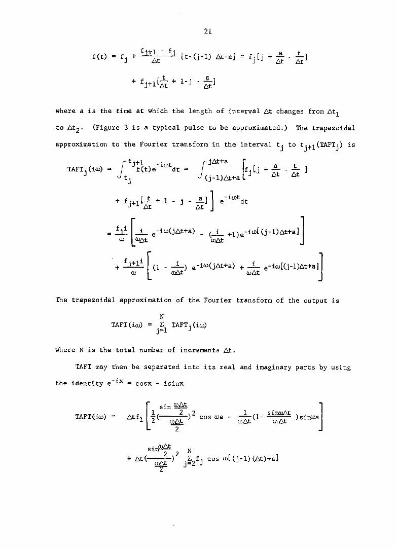
study. Given below is a summary of the trapezoidal approximation to the
Fourier transform (TAFT) given by Dreifke and Hougen (12) .
The straight line joining fj and fj+i is described by the equation

Figure 2. Differently shaped pulses
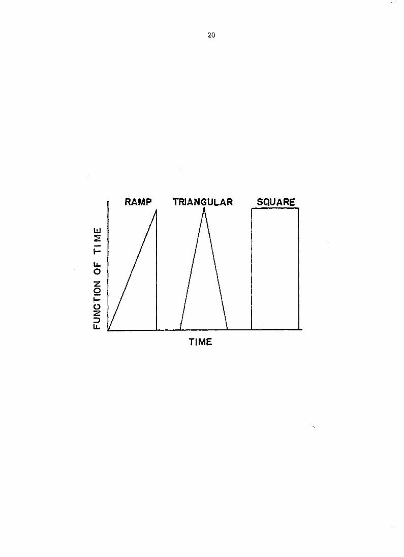
20
TRIANGULAR RAMP SQUARE
111 2
H
li. O
z o !-o z D U.
TIME
21
f(C) ° f j + [ t - ( J - l ) A t - » ] - f j t J + ^
+ 1-J - Z'
where a is the time at which the length of interval At changes from Atj^
to At2. (Figure 3 is a typical pulse to be approximated.) The trapezoidal
approximation to the Fourier transform in the interval tj to tj^j^(TAFTj) is
TAFT.(icJo) = f ^f^t)e"i"*dt = / ^ + At ' At ^
h
p jAt+a I"
(j-l)At+a
^ - hM
hi CD
_1_ jAt+a) _ X i +i)e-iw[(j-l)At+a] At U)At
+ £itli œ
(1 —) e-l(:)(jAt+a) + _i_ e-iœ[(j-l)At+a] oûAt mAt
The trapezoidal approximation of the Fourier transform of the output is
N TAFT(iœ) = L TAFT; (im)
j=l
where N is the total number of increments At.
TAFT may then be separated into its real and imaginary parts by using
the identity e"^^ = cosx - isinx
TAFT(iœ) = Atf^
sin
2'"~szr>^ jà"-
2 " + At(—^^^^) jZ^fj cos œ[(j-l) (At)+a]
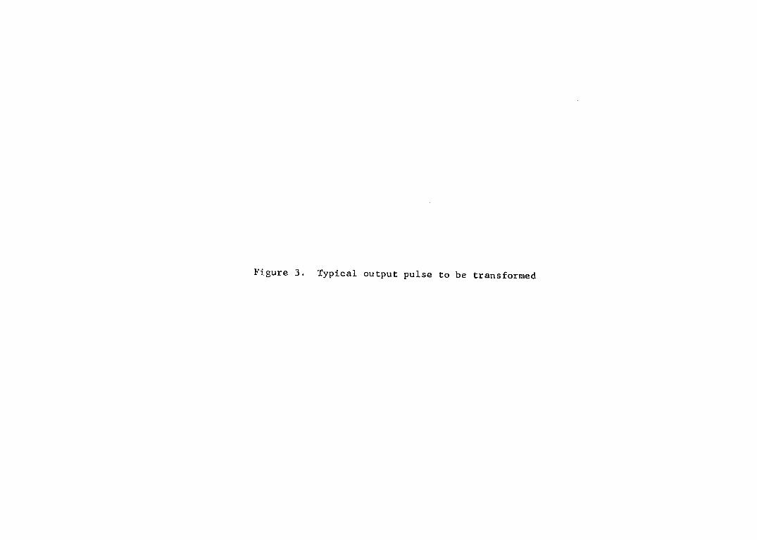
Figure 3. Typical output pulse to be transformed
FUNCTION OF TIME
£Z

24
+ Atf N+1
+ i < Atf
sin 2^
sin cD(NAt+a)
- A(SinD^/2^ sino» - —1— (1- .£iHyù£) cos cua 2 u)At/ 2 m At cuAt
+ &(SigwAt^2)2 L f . (-sinœ[ (j-l)At+a]) + mAt/2 j-2 J
Atf N+1 - i(SinmAt/^^2 sino)(NAt+a) 2 m At/2
+ (1- sinmAt^ cos a)(NAt+a) CO At m At
The above is in a suitable form for machine computing, given the values
of fj from the experimental data.
It has been stated that the pulse is made up of a spectrum of fre
quencies, but nothing has yet been mentioned about the relative amplitudes
of the various sinusoids (frequency content) which make up a pulse, or
what determines these amplitudes. Obviously, the height of any pulse
directly governs the magnitudes at all frequencies. Also, the width of
the pulse of any shape may be expected to influence the frequency content
of the pulse, since it is one of the limits of the integration to
determine the Fourier transform and the frequency content is equal to the
complex amplitude of the Fourier transform at a given frequency. The
shape of the pulse (square, triangular, etc.) is probably the most
important single criterion in determining the frequency content of a
25
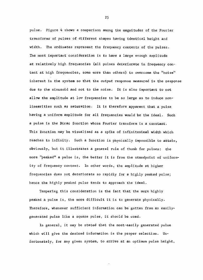
pulse. Figure 4 shows a comparison among the magnitudes of the Fourier
transforms of pulses of different shapes having identical height and
width. The ordinates represent the frequency contents of the pulses.
The most important consideration is to have a large enough amplitude
at relatively high frequencies (all pulses deteriorate in frequency con
tent at high frequencies, some more than others) to overcome the "noise"
inherent in the system so that the output response measured is the response
due to the sinusoid and not to the noise. It is also important to not
allow the amplitude at low frequencies to be so large as to induce non-
linearities such as saturation. It is therefore apparent that a pulse
having a uniform amplitude for all frequencies would be the ideal. Such
a pulse is the Dirac function whose Fourier transform is a constant.
This function may be visualized as a spike of infinitesimal width which
reaches to infinity. Such a function is physically impossible to attain,
obviously, but it illustrates a general rule of thumb for pulses: the
more "peaked" a pulse is, the better it is from the standpoint of uniform
ity of frequency content. In other words, the amplitude at higher
frequencies does not deteriorate so rapidly for a highly peaked pulse;
hence the highly peaked pulse tends to approach the ideal.
Tempering this consideration is the fact that the more highly
peaked a pulse is, the more difficult it is to generate physically.
Therefore, whenever sufficient information can be gotten from an easily-
generated pulse like a square pulse, it should be used.
In general, it may be stated that the most-easily generated pulse
which will give the desired information is the proper selection. Un
fortunately, for any given system, to arrive at an optimum pulse height.

Figure 4. Frequency content of pulses versus frequency

27
.0
SQUARE PULSE
>- 05
TRIANGULAR PULSE
RAMP PULSE
0 0 20 0
FREQUENCY, RADIANS/MINUTE

28
width, and shape is a trial-and-error procedure, and only by previous
experience or extreme good fortune is it possible to make an optimum
selection of a pulse on the first try, or even after several tries.
Normally, a good procedure would be trying square pulses of several
widths and heights and only if inconclusive data at high frequency are
obtained resorting to more difficult to generate pulses of higher ampli
tude at high frequency.
Limitations of Pulse Testing
Validity of linearity assumption
The pulse testing method has all of the limitations of dynamic
testing by frequency response methods, the fundamental one of which is
dependence on the accuracy of describing a system by linear ordinary
differential equations with constant coefficients (linearity). As ludi
crous as it may seem to attempt describing complicated, nonlinear phenomena
by such equations, the loss in accuracy in most cases is negligible if
the changes in operating variables are kept small enough. One example
which illustrates this is the case of a liquid level process. Consider
the liquid level system in Figure 5.
Material balance:
Input-Output = Accumulation
- 4° - A
Qj = Inflow, cubic feet/second
QQ = Outflow, cubic feet/second
A = Cross section of tank, square feet
h = Height of liquid in tank, feet
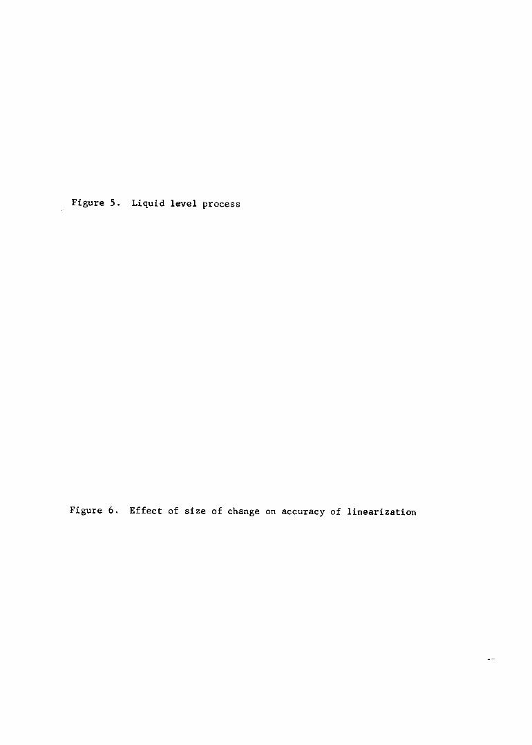
Figure 5. Liquid level process
Figure 6. Effect of size of change on accuracy of linearization

30
Q
H
— Qo
SMALL CHANGE IN H
LARGE CHANGE IN
H

31
t = time, seconds
Since = £(h) it may be seen that a first order differential
equation will result from this analysis.
It is well known that the expression relating outflow from an orifice
to liquid level is Qq = -k »/h but A •^ + k s/'h = is the result of this
analysis, giving a nonlinear differential equation to solve, an arduous
task. If, however, it is assumed that
Qq = -Ch, then
A -^ + Ch = is the result,
which is a linear equation with constant coefficients and easily solved.
Even though the assumption gives rise to error. Figure 6 shows that this
error is minimized by small changes in h. As the changes in h become
smaller, the chords representing the linearization become tangent lines
in the limit and represent the curve. It is therefore plain that linear
differential equations may be used to represent nonlinear phenomena to
a good approximation provided the changes are small enough.
Pulse testing compared to mathematical simulation
Direct mathematical simulation has the characteristic of forcing one
to know the assumptions and linearizations made in order to solve the
differential equations of the system. It has the distinct advantage
that, once the differential equations are solved, the solution is
directly applicable to all systems describable by the same differential
equations and boundary conditions. All that need be changed are the
parameters of the solution. It is a fact that this approach is best.
32
provided the solution of the differential equations actually represents
the dynamics of the system accurately. This is perhaps less often the
case than not, due to the extreme difficulty in deriving realistic
differential equations for complicated systems. As in the case of dynamic
testing, the assumptions inherent in the method often limit the applica
tion of the direct mathematical simulation. In summary, the following
points may be made:
1. Dynamic testing results in mathematical models which are neces
sarily limited to a narrow range of operating variables by the assumption
of linearity and to a specific piece of equipment. Direct mathematical
simulation gives rise to mathematical models which are not necessarily
limited by the assumption of linearity and are general for a class of
equipment describable by the same differential equations and boundary
conditions.
2. The assumption of linearity implicit in dynamic testing has the
compensation of generating a linear ordinary differential equation with
constant coefficients as a mathematical model for the system. Such an
equation is easily solved, so control system analysis and other studies
involving simulation are considerably simplified. Methods for direct
mathematical simulation range from analytical solutions (quite rarely)
through analog simulation to numerical integration using a digital
computer. Control analyses involving the use of a digital computer are
often more involved than are those using models from dynamic testing.
Pulse testing compared to sinusoidal forcing
Pulse testing as a means of deriving frequency response information
has the distinguishing aspects not only of reducing the experimentation

33
necessary for obtaining a useful amount of data, but of increasing the
laboriousness of converting time response data to frequency response data.
The calculation of the trapazoidal approximation to the Fourier transform
is most practical if a digital computer is available to handle the many
repetetive calculations involved.
The problem of obtaining satisfactory information at high frequencies
from pulse testing is not a severe one. There are sufficient degrees of
freedom in pulse size and shape that it is normally possible to cover
the frequencies of interest.
Perhaps as commanding a reason as any for dynamic testing by pulse
techniques is the great amount of information to be obtained from a
limited amount of experimentation. In an onstream piece of equipment,
the less experimentation, the less off-specification product produced, the
less disruption of production schedules, and the less expense. In a case
where 20 or more sinusoidal forcing runs would need to be made, with the
resultant ill effects on the productivity of the plant, a single pulse
test might produce an equal or greater amount of information. Pulse
testing may require no special equipment, since a square pulse is simple
to generate by, for example, the rapid turning of a valve fully-open to
fully-closed and back to fully-open. Arbitrarily-shaped pulses could be
generated by the turning of a valve as well. Sinusoidal inputs are
generated in many cases by ingeniously-contrived devices which may be
expensive, difficult to operate, and limited to low frequencies; in almost
every case they do not generate perfect sinusoids. In a number of situa
tions, in fact, a sinusoidal input cannot be generated at all.

34
It may be seen, therefore, that very few instances exist when pulse
testing could not be used. Pulse testing would be preferred over direct
sinusoidal forcing in nearly every situation in which a digital computer
is available.

35
EQUIPMENT
Characteristics of a Pulse Column
The pulse column is a development which makes possible separations
for which the separation factor (the ratio of the distribution coef
ficients of two materials) is too close to unity for such equipment as
packed columns. (A packed column would have to be very high due to the
large height of a transfer unit (HTU) in comparison to that of a pulse
column.) Also, the throughput per unit area in a pulse column is much
higher than for a packed column.
In general, HTU depends strongly upon the rate of generation of new
interfacial area. In the case of a packed column, this takes place as a
result of the inability of the discontinuous phase to wet the packing as
it rises through the column breaking up and recoalescing in the randomly-
distributed channels created by the packing. In the case of a pulse
column, the discontinuous phase is broken into small droplets as it is
forced through the sieve plates by the upstroke of the continuous
phase; these droplets then rise to the next sieve plate where they either
pass through or recoalesce. Some or all pass through if the pulse
stroke length is as large as or larger than the plate spacing. Those
droplets which do not pass through the plate recoalesce below it, and
none pass through if the pulse stroke length is much smaller than the
plate spacing. When all the solvent which passes through one plate on
the upstroke recoalesces below the next higher plate on the downstroke,
the column is said to be operating in the "mixer-settler" region. The
most usual condition is that some droplets pass through the next higher

36
plate and some recoalesce below it. At considerably higher pulse fre
quencies, the droplets formed are so small and the time between subsequent
upstrokes is so small as to allow little or no recoalescence. This con
dition is known as the "emulsion" region of operation.
The energy furnished by the cyclic pulsing of the continuous phase
makes possible a much smaller HTU by the higher rate of generation of new
interfacial area in comparison to a packed column, in which the energy
comes from buoyancy effects.
The pumping action of the pulsing mechanism in a pulse column makes
possible a much higher throughput per unit area than is possible through
gravity flow in a packed column. In fact, gravity flow in a pulse column
is normally impossible, since the interfacial tension of the discontinuous
phase in the presence of the continuous phase prevents the discontinuous
phase from flowing through the sieve plates by buoyancy alone.
In general, it may be stated that pulse columns are valuable for
close separations because of high throughput and small HTU. However, an
ordinary separation for which the separation factor is moderate to large
negates the advantage of small HTU and makes the high cost of operation
and the high initial cost of a pulse column major drawbacks. For this
reason, little usage of pulse columns in commercial operations has been
reported.
Experimental Pulse Column
The pulse column and associated equipment are described schematically
in Figure 7.

1
Figure 7. Schematic of pulse column

AGIO
TANK
COLUMN
SOLVENT
FEED
TANK
RAFFINATE
TANK
SOLVENT OVERFLOW
TANK

39
Pertinent dimensions are given below:
Column height
Plate section height
Column inside diameter
Plate-to-plate distance
Plate hole diameter
Pulse pump range
20 feet - 1/2 inch
14 feet - 11 inches
3 inches
21/4 inches
I/I6 inch
19-200 cycles/minute; 0-3 inches stroke length in
column
0-20 gallons/hour
550 gallons
Flow rate range
Total liquid storage capacity
The column is of a design similar to that used by Burkhart (3) and
is described in detail by Biery (2).

40
PROCEDURE
Liquid-Liquid Extraction System
A system of water-nitric acid-tributyl phosphate-paraffin was used
in the pulse column. The tributyl phosphate-paraffin consisted of a 1:1
volumetric mixture of tributyl phosphate furnished by Commercial Solvents
Corp. and Varsol No. 1 (a purified fraction of nonane and decane sold by
Humble Oil and Refining Co.). One function of the paraffin dilution of
tributyl phosphate is to cause the specific gravity of the solvent phase
to be smaller than that of the aqueous phase. The advantage of the system
for this study was that the materials were available and no equipment
changes were needed. The reasons cited by Biery (2) for the selection of
the system for his study were that the aqueous phase could be continuously
analyzed with conductivity cells, the organic phase is reasonably low in
volatility, the nitric acid concentration in both the aqueous phase and
the organic phase is determinable by standard titration techniques,
materials of construction are not a major problem with nitric acid, and
the mutual solubility between the aqueous and the organic phase is small
so that the acid-free flow rates of aqueous and organic are nearly
constant and give straight operating lines.
Operation of Column
Because it is possible to introduce feed at four separate points in
the column, it is possible to maintain the interface such that 100 per cent,
75 per cent, 50 per cent, and 25 per cent of the plate section height is
utilized. Due to the fact that the feed tap corresponding to 50 per cent
41
of the plate section height is at eye level on the operating platform of
the pulse column, and better interface control is thus possible with the
interface at eye level, all the runs reported in this study have been
made utilizing 50 per cent of the plate section height, which corres
ponds to a 40-plate column.
Runs to determine the effects of various independent variables on
the raffinate acid concentration were made in the following fashion: The
column was allowed to come to steady conditions as indicated by a con
stant value of the raffinate acid concentration, then the variable in
question was pulsed and the column was allowed to return to steady condi
tions after the pulse. The total time of transient conditions was 1 to 2
hours. All variables other than the one being deliberately changed were
maintained constant as nearly as possible.
Interface control was accomplished by maintaining a constant feed
rotameter reading and adjusting the raffinate flow rate to maintain the
interface at a constant level. It is possible to maintain a constant
raffinate rotameter reading and adjust the feed rate to maintain a
constant interface level, but because the acid-free flow rate must be
constant to obtain a straight operating line and the acid concentration
of the raffinate is continuously varying during the transient portion of
the run, the raffinate rotameter reading corresponding to a constant
acid-free flow rate would be continuously varying also. (The rotameter
indicates total flow rate rather than acid-free flow rate.) Since the
feed acid concentration was constant, the rotameter reading corresponding
to a given acid-free flow rate was constant. The organic phase was easily
kept at a constant rate by maintaining the inlet rotameter at a constant

42
value. The solvent overflowed continuously from the top of the column as
it was displaced from below.
Average flow rates were determined by before-and-after measurements
of level in the feed tanks. Knowledge of the area of the tanks made
possible flow rate determinations to a reasonable degree of accuracy
(+ 3 per cent as reported by Biery (2) ).

43
RESULTS
The results of ten pulse tests, designated as Runs 1 through 10, are
reported in the following paragraphs.
In the tests analyzed the effects of changes in column pulse fre
quency, aqueous phase flow rate, organic phase flow rate, and aqueous
feed concentration on the response of the raffinate acid concentration
were evaluated.
All pulse tests reported were carried out at an aqueous phase flow
rate of 68 + 7 pounds acid-free phase/hour and at an organic phase flow
rate of 150 + 15 pounds acid-free phase/hour. The organic feed concentra
tion was zero, and the steady-state aqueous feed concentration was 0.1
+ 0.05 pounds nitric acid/pounds acid-free phase. Runs 1 and 2 were made
at a column pulse frequency of 20 cycles per minute, and the remainder of
runs reported were made at 40 cycles per minute.
The pulse tests to ascertain the effects of column pulse frequency,
aqueous phase flow rate, organic phase flow rate, and aqueous feed con
centration were analyzed in pairs; within each pair both an increase and
a decrease in the variable were made.
The frequency response data for the pulse tests were calculated in
the form of tabulated logarithm of amplitude ratio (log AR) and phase
angle (PA) versus frequency (cu) . These data were plotted as Bode diagrams
for the runs reported.
For those pulse tests in which there was no intent or in which it was
not possible to develop models for the control analysis, the data were
left in the form of the above mentioned Bode diagrams. In those tests
44
made for the purpose of developing models for the control analysis, the
data were replotted to make possible the determination of the parameters
of the response. The new plots were made using frequency ratio (the
ratio of frequency to break frequency) for the frequency coordinate,
rather than frequency itself. This replotting makes every first-order
profile identical, regardless of time constant, and every second-order
profile of a given damping ratio the same, regardless of natural frequency.
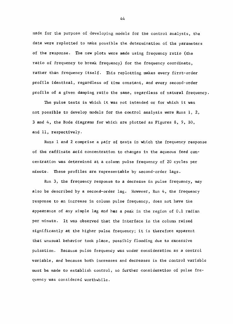
The pulse tests in which it was not intended or for which it was
not possible to develop models for the control analysis were Runs 1, 2,
3 and 4, the Bode diagrams for which are plotted as Figures 8, 9, 10,
and 11, respectively.
Runs 1 and 2 comprise a pair of tests in which the frequency response
of the raffinate acid concentration to changes in the aqueous feed con
centration was determined at a column pulse frequency of 20 cycles per
minute. These profiles are representable by second-order lags.
Run 3, the frequency response to a decrease in pulse frequency, may
also be described by a second-order lag. However, Run 4, the frequency
response to an increase in column pulse frequency, does not have the
appearance of any simple lag and has a peak in the region of 0.1 radian
per minute. It was observed that the interface in the column raised
significantly at the higher pulse frequency; it is therefore apparent
that unusual behavior took place, possibly flooding due to excessive
pulsation. Because pulse frequency was under consideration as a control
variable, and because both increases and decreases in the control variable
must be made to establish control, no further consideration of pulse fre
quency was considered worthwhile.
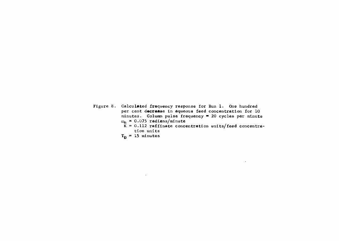
Figure 8. Calculated frequency response for Run 1. One hundred per cent decrease in aqueous feed concentration for 10 minutes. Column pulse frequency = 20 cycles per minute (% = 0.075 radians/minute K = 0.112 raffinate concentration units/feed concentra
tion units Tjj = 15 minutes

0
-10
TJ % >
-20 %
> z o r
-30 o m o 73 m
-40 S
-50
10"® 10"® 10"' , 10®
FREQUENCY, RAOIANS/MINUTE

1
Figure 9. Calculated frequency response for Run 2. One hundred per cent increase in aqueous feed concentration for 10 minutes. Column pulse frequency = 20 cycles per minute
=» 0.218 radians/minute K = 0.080 raffinate concentration units/feed concentra
tion units Tj) =* 5 minutes

48
PHASE ANGLE, DEGREES 0 o O OJ ro ^
1 I I
o O
r g g
oiivd aaniiidwv

Figure 10. Calculated frequency response for Run 3. One hundred per cent decrease in column pulse frequency for 5 minutes. Steady state column pulse frequency = 40 cycles per minute
*• 0.070 radians/minute K = 2.88 X 10"4 raffinate concentration units/cycles
per minute Td = 0

.—3
-10
r"4
-30 m w
<10 — 40 rn
-50
>-3 10"'
o FREQUENCY, RADIANS/MINUTE

Figure 11. Calculated frequency response for Run 4. Fifty per cent increase in column pulse frequency for 5 minutes. Steady state column pulse frequency = 40 cycles per minute * not determinate
K = 3. xlO"^ raffinate concentration units/cycles per minute

20
—3o
- 40 m
-50
10" 10"' FREQUENCY, RADIANS/MINUTE
53
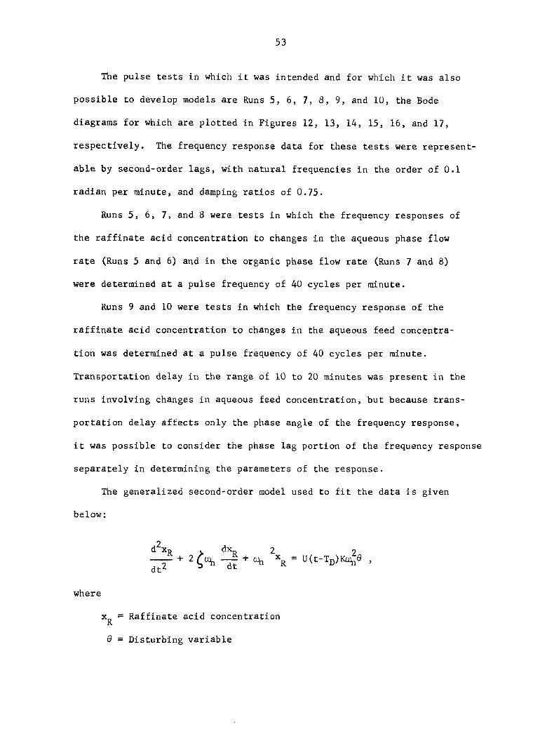
The pulse tests in which it was intended and for which it was also
possible to develop models are Runs 5, 6, 7, 8, 9, and 10, the Bode
diagrams for which are plotted in Figures 12, 13, 14, 15, 16, and 17,
respectively. The frequency response data for these tests were represent-
able by second-order lags, with natural frequencies in the order of 0.1
radian per minute, and damping ratios of 0.75.
Runs 5, 6, 7, and 8 were tests in which the frequency responses of
the raffinate acid concentration to changes in the aqueous phase flow
rate (Runs 5 and 6) and in the organic phase flow rate (Runs 7 and 8)
were determined at a pulse frequency of 40 cycles per minute.
Runs 9 and 10 were tests in which the frequency response of the
raffinate acid concentration to changes in the aqueous feed concentra
tion was determined at a pulse frequency of 40 cycles per minute.
Transportation delay in the range of 10 to 20 minutes was present in the
runs involving changes in aqueous feed concentration, but because trans
portation delay affects only the phase angle of the frequency response,
it was possible to consider the phase lag portion of the frequency response
separately in determining the parameters of the response.
The generalized second-order model used to fit the data is given
below:
d^xj, dx 2 2 + <% U(t-TD)K4;9 ,
where
X = Raffinate acid concentration R
9 = Disturbing variable

Figure 12. Calculated frequency response for Run 5. Fifty per cent decrease in aqueous phase flow rate for 5 minutes. Column pulse frequency = 40 cycles per minute
0.75 = 0.265 radians/minute
K = 3.54x10"^ raffinate concentration units/per cent rotameter reading
Td - 0
(Solid lines on graphs are second order profiles)

10 -5
10 - 4 _
OC
u o 3 H
Q. 5 <
lÔ"
0
- - I 0
"D DC
• 2 0 5 m > z G)
30 jij
O m o
3D
.40 m (fi
50
10" ' 10'
FREQUENCY RATIO
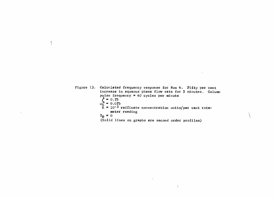
Figure 13. Calculated frequency response for Run 6. Fifty per cent increase in aqueous phase flow rate for 5 minutes. Column pulse frequency = 40 cycles per minute / » 0.75 0^ » 0.075 K = 10"3 raffinate concentration units/per cent rota
meter reading Td = 0
(Solid lines on graphs are second order profiles)

i
20 >
40CU
10 -2 10"' 10°
FREQUENCY RATIO 10'
Ln
1
Figure 14. Calculated frequency response for Run 7. Fifty per cent decrease in organic flow rate for 2 l/2 minutes. Column pulse frequency = 40 cycles per minute / = 0.75 = 0.090 radians per minute
K =• 3.5x10"^ raffinate concentration units/per cent rotameter reading
Td = 0
(Solid lines on graphs are second order profiles)
I

--ID
aoi m
o
'30 m
o m o 33
'40m U)
- -50
10"' 10®
FREQUENCY RATIO

Figure 15. Calculated frequency response for Run 8. Ten per cent increase in organic phase flow rate for 5 minutes. Column pulse frequency = 40 cycles per minute / = 0.75 = 0.090 radians per minute
K = 4.4x10"^ raffinate concentration units/per cent rotameter reading
Td = 0
(Solid lines on graphs are second order profiles)

.-3
,-4
-30 P
-40
-50
,-i
FREQUENCY RATIO

Figure 16. Calculated frequency response for Run 9. One hundred per cent decrease in aqueous feed concentration for 2 l/2 minutes. Column pulse frequency =» 40 cycles par minute
a: - u.u 5 radians per minute K " 0.354 raffinate concentration units/feed concentra
tion units Tjj = 21 minutes
(Solid lines on graphs are second order profiles)

I0~®
Ï0~
o o o
10"' - 10'
FREQUENCY RATIO
—1-0
3 o i m
o
•30 S
O m o
:o _ m
40 m en
- -50
10'

Figure 17. Calculated frequency response for Run 10. One hundred per cent increase in aqueous feed concentration for 5 minutes. Column pulse frequency = 40 cycles per minute / - 0.75
= 0.115 radians per minute K » 0.229 raffinate concentration units/feed concentra
tion units Tg =• 13 minutes
(Solid lines on graphs are second order profiles)

10 - 0
10-O
h-< CC
Lui O =) H
a. Z
" 10"
o
— —10
J > z o r
m -30
Ln
-40
o m o 3) m m ùi
lO 1— 2 10"' 10°
FREQUENCY RATIO
- —50
10'

6 6
^ = Damping ratio
= Natural frequency
K = Zero-frequency gain
t = Time
Tjj = Delay time
U(t-Tj)) = Unit step function (0 when t < Tp, 1 when t > Tg) .
The second-order models obtained from the frequency responses as
well as the adjusted models (discussed later) are presented in Table 1.
To test the models from the frequency response, a second-order model
was programmed on a PACE TR-48 analog computer, and attempts were made to
reproduce the original time response data. Figures 18, 19, and 20 are
comparisons of the simulations of the six models to the experimental data.

Table 1. Summary of models from pulse testing (for a 3-inch diameter, 40-plate pulse column)^
Variable changed Frequency response model Adjusted model
Aqueous phase flow rate L
d^Xn dXp ^ + 0.1123 —^ + 0.00056%%
dt2 dt ^
= 5.64 X 10"
+ 0.197 dt2 dt
+ 0.0172x% = 1.102 X lO'^L
Aqueous phase flow rate L
S_p + U.4 is + 0.0711 XR dt^ dt
= 2.46 x 10"5L
0 .45 0 . dt2 dt
= 2.61 X lO-^L
09x R
Organic phase flow rate V
IZR + 0.135 + 0. dt^ dt
= -2.80 x lo -^v
OOBlx R + 0.81 + 0.291Xr
dt2 dt ^
= -2.72 x 10⁻⁴v
Organic phase flow rate V
d^XR dXR + 0.135 —- + 0.0081x_
dt2 dt ^
= -2.80 X 10"^V
d^XR dXR —^ + 0.81 —- + 0.291 xn dt2 dt
= -10-^V
^Aqueous phase flow rate ~ 68 + 7 pounds acid-free phase/hour. Organic phase flow rate =
150 + 15 pounds acid-free phase/hour. Organic feed concentration = 0. Steady-state aqueous feed concentration -0.1+ 0.05 pounds HNO^/pound acid-free phase.

Table 1. (Continued)
Variable changed Frequency response model Adjusted model
Aqueous feed concentration
d Xtj dXn —+ 0.1315 —^ + 0.00882xr
dt dt
= 3.06 X 10⁻³xn U(t-21)
—+ 0.0876 + 0.00392XR dt^ dt
= 2.39 x 10⁻³x- U(t-21)
Aqueous feed concentration x?
d^x dXn ^ + 0.1726 —± + 0.0132xs
dt2 dt ^
= 2.79 X 10⁻³xp U(t-13)
2 d Xp dxp —+ 0.1726 —- + 0.0132xo dt2 dt ^
= 3.44 X 10- xp U(t-13)

Figure 18a. Comparison of simulations to time response for Run 5. Decrease in aqueous phase flow rate
(Adjusted model generated by changes in natural frequency of frequency response model)
Figure 18b. Comparison of simulations to time response for Run 6. Increase in aqueous phase flow rate
(Adjusted model generated by changes in natural frequency of frequency response model)

70
FREQUENCY RESPONSE MODEL
ADJUSTED MODEL
20 30 TIME; MINUTES
40 50 2
3
FREQUENCY RESPONSE MODEL 2
0

Figure 19a. Comparison of simulations to time response for Run 7. Decrease in organic phase flow rate
(Adjusted model generated by changes in natural frequency of frequency response model)
Figure 19b. Comparison of simulations to time response for Run 8. Increase in organic phase flow rate (Adjusted model generated by changes in natural frequency of frequency response model)

72
m O
W C/) <
£ U LU q: u_
o <
^ 1 -
CO o z 3 O a.
2 -
I - ADJUSTED MOCIL
5 ° <
O z 3 O û.
\ O
FREGUÉNCY RESPONSE MODEL
10 20 30 40
TIME, MINUTES
50
ADJUSTED MOCZL
FREQUENCY RESPONSE MODEL
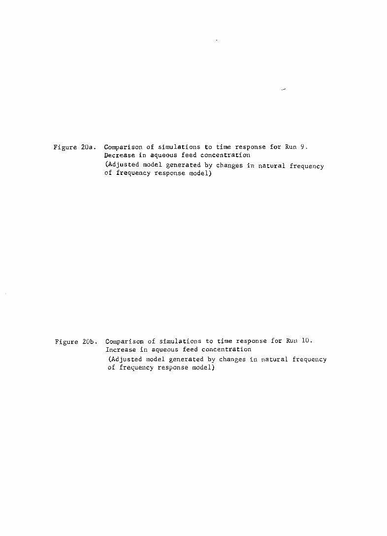
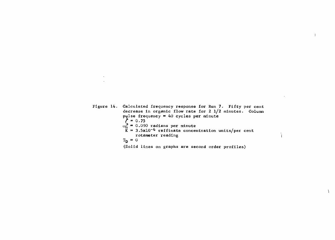
Figure 20a. Comparison of simulations to time response for Run 9. Decrease in aqueous feed concentration
(Adjusted model generated by changes in natural frequency of frequency response model)
Figure 20b. Comparison of simulations to time response for Run 10. Increase in aqueous feed concentration
(Adjusted model generated by changes in natural frequency of frequency response model)
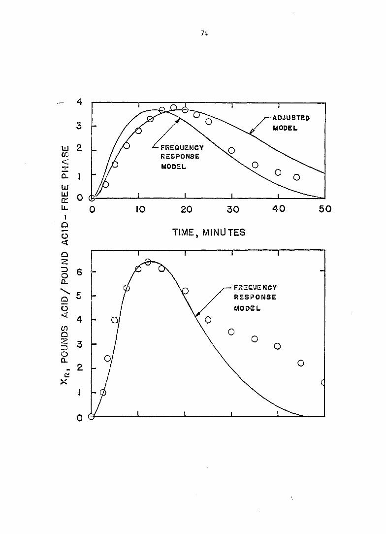
74
ADJUSTED MODEL
FREQUENCY RESPONSE MODEL
FRECUSNCY RESPONSE MODEL

75
DISCUSSION OF RESULTS
There apparently have been no attempts by other workers to reproduce
experimental time response data by use of the models obtained from pulse
testing. Pulse testing of systems having known responses has given
verification of pulse testing procedures. However, pulse testing a com
plex system of unknown response and attempting to reproduce the system
time response with the model obtained by pulse testing, such as was done
in this study, is subjecting the pulse testing method to a much more
critical test than has been done previously. The experience with pulse
testing in this study leads to the conclusion that pulse testing is a
promising method for obtaining dynamic models for complex processes, but
that application of this method without due consideration of certain
weaknesses of the method is likely to produce results of lesser quality
than expected. The major weakness is the fact that the log amplitude
ratio and the phase angle data points followed smooth curves at low fre
quencies, but began to scatter approximately one order of magnitude above
the break frequency. This readily identified second-order responses, but
left the possibility of higher-order responses speculative.
Because the models from pulse testing were variable in their abil
ities to simulate time response data, it was decided to adjust the
natural frequencies of the models in order to better simulate the
initial rise in the experimental pulse, since this was thought to be
analogous to the simulation of step changes. The adjusted models are
compared to experimental data in Figures 18, 19, and 20. It can be
seen that in the majority of cases the response to the adjusted model

76
returned to steady state prior to the return of the experimental data.
Because of this, it was conjectured that higher-order models would fit
the experimental time response better than the second-order models did.
When a third-order model was made by adding a first-order lag to an
adjusted second-order model, the simulation was found to be marginally
improved. Therefore, an improvement would be achieved each time the
order of the assumed model is increased by one, with an additional
parameter being added. It is possible that a fifth-order model would have
approached the experimental time response closely. However, adjusting
five parameters to an optimum would be extremely difficult. Fitting
fifth-order models would be much simpler by determining the five
parameters from frequency response data rather than by arbitrarily
adjusting them to an optimum.
The previous discussion suggests that there are two general ap
proaches to the fitting of linear models to experimental time response
data. These are:
1. Pulse testing
2. Assuming an arbitrary linear model to hold and adjusting the
parameters of this model, using an analog computer, until the
solution of the model simulates the time response data.
Which of the two methods is better would depend upon the order of the
model. For models no higher than third-order. Method 2 would probably
be at least as good as pulse testing, and require no more effort. For
models higher than third-order, pulse testing would probably be better,
due to the difficulties in adjusting parameters.
If pulse testing is used, the weakness which arises because of

77
scattered data at high frequency must be alleviated. Scattering takes
place, at least in part, as a result of the ratio of the frequency con
tent of the pulse to the noise of the system becoming too small. The
frequency at which the points began to scatter was therefore dependent
upon the frequency content of the pulse, which should be maximized, and
upon the noise, which should be minimized. If there is not enough
frequency content to overcome noise, scatter is inevitable. Therefore,
the frequency range may be extended by using pulses of higher frequency
content than the square pulses used in this study and by reducing the
level of noise in the system.
Pulses of higher frequency content than square pulses may be gen
erated mechanically by making the stem of a linear valve the follower
of a cam having the pulse cut into it. Pulses of no particular mathe
matical shape, but having high frequency content, may be generated
manually provided the necessary recording equipment is available. A
considerable improvement in frequency content is possible with a reason
able expenditure of effort.
Reducing the level of noise may be achieved by better instrumenta
tion of the system, thus reducing the fluctuations in variables wiiich
are presumed constant in the pulse testing analysis. Interface level
control and flow rate control of the aqueous and organic streams would
eliminate a great deal of variability in both the interface level and in
the flow rates, with a resultant increase in the precision of time
response data. In order to take advantage of such an increase in
precision, the continuous concnetration recorder would need to make a
continuous trace on the chart paper, the zero setting of the recorder

78
should be adjustable, and recorder sensitivity would need to be adjust
able so the response would fill the span of the recorder. Faster chart
speeds and more rapid pen response would be beneficial, as well.
In the second-order models obtained by pulse testing the damping
ratio was found to be 0.75 in every case. The method of determining
the damping ratio has a maximum error of 0.05; therefore, there is
little doubt of the underdamped nature of the models. Because feedback
must be present for underdamping to exist, there must be feedback in
the pulse column.
Considering the column to consist of a number of perfectly mixed
stages in series, the material balance equations over the nth stage are:
"n = V n+l - Vyn + KG*(yn* " Yn)
dx^ — Lx^_l - LXn - KG*(yn* " Yn)
where = Holdup of organic phase per foot of column height, pounds/foot
hjj = Holdup of aqueous phase per foot of column height, pounds/foot
y^ = Concentration in organic phase in n stage, dimensionless
x^ = Concentration in aqueous phase in n Jth stage, dimensionless
YYI* - Concentration in n stage which would be in equilibrium with , dimensionless
t = Time, minutes
V = Flow rate of organic phase, pounds/minute
L = Flow rate of aqueous phase, pounds/minute
Kga = Mass transfer coefficient, pounds/(minute)(foot)

79
The differential equations for a single stage may be diagrammed as
in Figure 21. It may be seen that follows a path to y^ which sub
sequently follows a path to y^-i, yn-2» etc., each of which follows a
path to Xn-2) etc., respectively. Feedback therefore exists due
to the countercurrent flow of aqueous and organic phases and the inter
phase mass diffusion.
It is obvious that transportation delay would be involved in the
response to changes in the aqueous feed acid concentration, since a
disturbance in the concentration of the aqueous feed must flow through
the column before it reaches the raffinate outlet to be measured.
Longitudinal mass diffusion of solute causes the disturbance to be
measured earlier than the plug flow time (the time of flow of a particle
flowing the length of the column at the superficial velocity of- the
aqueous phase) .

Figure 21. Block diagram for differential equations of pulse column

- DENOTES AN OPERATION
Q - DENOTES A SUM
N + l
82
CONTROL ANALYSIS
Feedback control has long been the standard in industrial process
control because of its stability in most situations and because a good
mathematical model of the system is not essential to its application.
However, large lags or transportation delays can cause sluggish response
to load changes, since substantial errors can develop before the error can
be sensed and corrected. Figure 22 is a block diagram of a feedback
control loop for the pulse column.
The intent of feed-forward control is to speed up the response of a
control loop to such a point that no errors in the controlled variable
are allowed to take place. Figure 23 shows a feed forward control loop.
Block diagram algebra shows that, if there is to be no error in the
controlled variable, the transfer function for the feed-forward controller
must be - , so that, for the successful application of feed-PROGESS
forward control, models for both the load and the process must be known
to a much higher level of accuracy than for the case of feedback control.
Since no mathematical model is perfect, a feedback control loop must be
added to correct for imperfections in the mathematical models. Figure
24 shows this block diagram.
The only independent column variables which may reasonably be used
as control variables are the column pulse frequency the organic phase
flow rate, and the aqueous phase flow rate, since the other independent
variables may not be conveniently manipulated. All independent variables
other than the control variable are loads if they are subject to
perturbations during normal column operation. Two of the objectives of

Figure 22. Block diagram for feedback control
Figure 23. Block diagram for feed forward control
Figure 24. Block diagram for combined feedback and feed forward control
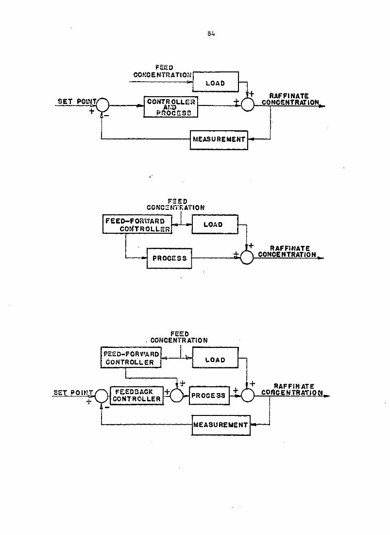
84
FEED CONCENTRATION
LOAD
SET POINT/^ CONTROLLER AND
PROCESS
CONTROLLER AND
PROCESS
RAF Fl NATE CONCENTRATION.
MEASUREMENT
FEED ATION
RAFFINATE CONCENTRATION
LOAD
PROCESS
FEED-FORWARD CONTROLLER
FEED CONCENTRATION
SET POIK
FEED-FORWARD V-, LOAD CONTROLLER LOAD
r
CONTROLLER PROCESS LtO RAFFINATE
CONCENTRATION
MEASUREMENT MEASUREMENT
85
this control analysis were the determination of the best control variable
and of what the loads are.
The major consideration in selecting the best control variable would
be the rapidity of the response of the controlled variable, raffinate acid
concentration, to changes in the control variable. Reference to the models
in Table 1 shows that the raffinate acid concentration responds most
rapidly to the organic phase flow rate (the natural frequency is largest).
Therefore the organic phase flow rate was selected as the control variable.
It is assumed for the purposes of this study that aqueous feed acid
concentration is the only load. It is further assumed that the control
value on the organic feed line and the measurement device for the
raffinate acid concentration each have transfer functions which are
simple gains (This is reasonable enough in light of the large time
constants involved in the process and in the load.) The transfer func
tion of the controller is the sum of the transfer functions of the propor
tional, integral, and derivative modes.
The control loop was simulated on the analog computer using the
adjusted second-order models obtained in this study. The analog diagram
used is in Figure 25.
The error caused by a step change in the aqueous feed acid concen
tration versus time was observed over wide ranges of proportional band,
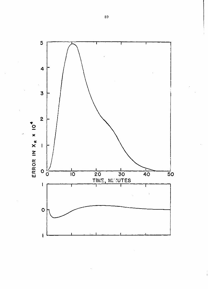
reset rate, and derivative time by use of the repetative operation mode
of the computer and an oscilloscope. Figure 26 shows the error-time
curve for integral control alone. The system is stable over a rather wide
range of reset rate, with the time of return to zero error being a minimum
at the value used. The addition of proportional control to integral
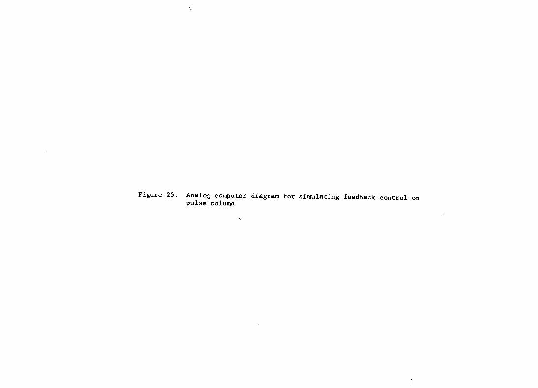
Figure 25. Analog computer diagram for simulating feedback control pulse column

1
15
B
0.239
E
0 9
do •Vl
KX ijyidr
M
o- MX
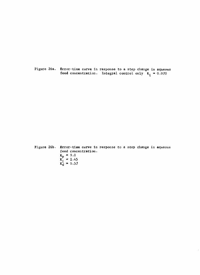
Figure 26a. Error-time curve in response to a step change in aqueous feed concentration. Integral control only = 0.070
Figure 26b. Error-time curve in response to a step change in aqueous feed concentration. Kp = 9.0
= 2.45
Kd = 0.57
89
90
'"rr.trcl nt thic couscq tne curve to flatten and the time of
return to zero error to be longer. Derivative control added to the optimum
integral control caused an initial overcorrection, which would tend to
minimize the integral of the error by the negative values of the error
cancelling the positive values. Combinations of all three modes were
tried until an optimum was found in which the integral of the error was
nearly zero, the integral of the error squared was small and the time of
return to zero error was small. Figure 27 is the error-time curve for
this optimum combination.
Di Liddo and Walsh (9) show the error time curves for integral
control alone and for proportional plus integral control. The curve
presented for integral control is qualitatively similar to Figure 26,
and the curve given for proportional plus integral control shows a
flattening from the curve for integral control and a lengthening of
the time of return to zero error, as was observed in this study. This
convergence of two radically different approaches to the control of a
pulse column lends credence to the results of both studies.

91
CONCLUSIONS AND RECOMMENDATIONS
The following conclusions have been made on the basis of the
results of this study:
1. Underdamped second-order dynamic models with no transportation
delay were found to represent the response of the raffinate acid concen
tration to changes in aqueous phase flow rate and in organic phase flow
rate. Underdamped second-order dynamic models with transportation delay
times from 10 to 20 minutes were found to represent the response of the
raffinate acid concentration to changes in the aqueous feed concentra
tion .
2 Pulse testing as a technique for obtaining dynamic models for
a pulse column is capable of good results. However, in this study,
equally good results could have been obtained with equal facility by
fitting the response of an arbitrary second-order model to the time
response data, using an analog computer.
3. It is likely that conventional three-mode control would be
stable at the settings arrived at in the control analysis, since
normal operating perturbations are quite small, and the system would
be nearly linear and free from interactions when small changes are
involved.
The following recommendations are made, based on the results of
this study:
1. Pulse testing should be applied only to systems for which the
time response data can be recorded with precision and for which changes
in variables other chan the one being pulsed are minimized.

92
2. liie empirical method of fitting the response of a second-order
or a third-order model to experimental response should be considered as
a desirable alternative to pulse testing when the conditions in recom
mendation 1 are not met.
3. If further pulse tests are carried out on the experimental pulse
column, it should be modified by the use of flow rate control on the feed
streams and of interface level control. Also, the continuous concentra
tion recorder should be modified to improve the precision of recording
time response data. Runs utilizing pulses of high frequency content,
such as triangular or ramp pulses, should be made.
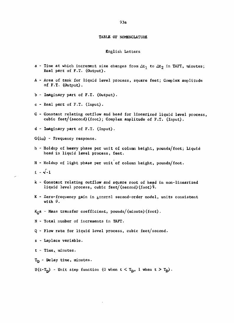
93a
TABLE OF NOMENCLATURE
English Letters
a - Time at which increment size changes from Atj^ to At2 in TAFT, minutes; Real part of F.T. (Output).
A - Area of tank for liquid level process, square feet; Complex amplitude of F.T. (Output).
b - Imaginary part of F.T. (Output).
c - Real part of F.T. (Input).
C - Constant relating outflow and head for linearized liquid level process, cubic feet/(second)(foot); Complex amplitude of F.T. (Input).
d - Imaginary part of F.T. (Input).
G(ico) - Frequency response.
h - Holdup of heavy phase per unit of column height, pounds/foot; Liquid head in liquid level process, feet.
H - Holdup of light phase per unit of column height, pounds/foot.
i - V-1
k - Constant relating outflow and square root of head in non-linearized liquid level process, cubic feet/(second)(foot)^.
K - Zero-frequency gain in general second-order model, units consistent with 0.
Kga - Mass transfer coefficient, pounds/(minute)(foot).
N - Total number of increments in TAFT.
Q - Flow rate for liquid level process, cubic feet/second.
s - Laplace variable.
t - Time, minutes.
Tjj - Delay time, minutes.
U(t-Tjj) - Unit step function (0 when t < Tg, 1 when t > Tjj) .

93b
V - riuw ittte or iignc phase, pounds/minute.
X - concentration in heavy phase, dimensionless.
y - Concentration in light phase, dimensionless.
y* - Concentration in light phase which would be in equilibrium with x, dimensionless.
z - Distance through column, feet.
Greek Letters
A - Denotes an increment in the variable it precedes. @2 ~ Phase angle for F.T. (Output).
@2 " Phase angle for F.T. (Input).
0Q - Laplace-transformed output.
8^ - Laplace-transformed input.
0 - Disturbing variable in general second-order model, units consistent with K.
^ - Damping ratio, dimensionless.
0) - Frequency, radians/minute.
- Natural frequency in general second-order model, radians/minute.
L - Denotes a summation.
Subscripts
F - Feed.
1 - Input.
j - Summation index for TAFT.
o - Output.
R - Raffinate.

94
LITERATURE CITED
1. Bates, H. T. and J. C. Webb. Nonlinear controller for underdamped systems. Chemical Engineering Progress 57, No. 9: 49-53. 1961.
2. Biery, J. C. The transient startup behavior of a liquid-liquid extraction pulse column. Unpublished Ph.D. thesis. Ames, Iowa, Library, Iowa State University of Science and Technology. 1961.
3. Burkhart, L. E. Pulse column design. Unpublished Ph.D. thesis. Ames, Iowa, Library, Iowa State University of Science and Technology. 1958.
4. Ceaglske, N. H. Automatic process control for chemical engineers. New York, N.Y., John Wiley and Sons, Inc. cl956.
5. Chambliss, C. W. Dynamic response of a continuous differential refractometer. Unpublished M.S. thesis. Ames, Iowa, Library, Iowa State University of Science and Technology. 1963.
6. Chestnut, H. and R. W. Mayer. Seirvomechanisras and regulating system design. 2nd ed. Vol. 1. New York, N.Y., John Wiley and Sons, Inc. cl959.
7. Clements, W. C., Jr. and K. B. Schnelle, Jr. Pulse testing for dynamic analysis. Industrial Engineering and Chemistry Process Design and Development 2: 94-102. 1963.
8. Deekshatulu, B. L. How to evaluate harmonic response of non-linear components. Control Engineering 10, No. 10: 53-56. 1963.
9. Di Liddo, B. A. and T. J. Walsh. Computer simulation of pulse columns. Industrial and Engineering Chemistry 53: 801-804. 1961.
10. Doebelin, E. 0. Dynamic analysis and feedback control. New York, N.Y., McGraw-Hill Book Co., Inc. cl962.
11. Draper, C. S., W. McKay, and S. Lees. Instrument engineering. Vol. 2. New York, N.Y., McGraw-Hill Book Co., Inc. 1953.
12. Dreifke, G. E. and J. 0. Hougen. Experimental determination of system dynamics by pulse methods. American Institute of Chemical Engineers Joint Automatic Control Conference 1963: 608-633. 1963.
13. Grensted, P. E. W. Analysis of the transient response of non-linear control systems. American Society of Mechanical Engineers Transactions 80: 427-432. 1958.

95
14. Kiotuer, K.. How to obtain describing functions for non-linear feedback systems. American Society of Mechanical Engineers Transactions 79: 509-512. 1957.
15. Loeb, J. M. Survey of mathematical methods for non-linear control systems. American Society of Mechanical Engineers Transactions 80; 1439-1450. 1958.
16. Savant, C. J. Basic feedback control system design. New York, N.Y., McGraw-Hill Book Co., Inc. cl958.
17. Stout, T. M. Basic methods for non-linear control system analysis. American Society of Mechanical Engineers Transactions 79: 497-507. 1957.
18. Watjen, J. W. and R. M. Hubbard. Hie dynamic behavior of a pulsed-plate extraction column. American Institute of Chemical Engineers Journal 9: 614-619. 1963.
96
ACKNOWLEDGMENTS
The author wishes to express his appreciation to Dr. M. A. Larson
for his guidance in all phases of this project.
Financial assistance from the National Science Foundation, the Iowa
Engineering Experiment Station, and the E. I. du Pont de Nemours and
Company Grant-in-Aid is gratefully acknowledged.
Top Related