


Languages
Pages
Legal


PSU Friday Transportation Seminar, 15 May 2015
Kelly J. Clifton, PhD *
Patrick A. Singleton*
Christopher D. Muhs*
Robert J. Schneider, PhD†
* Portland State Univ. † Univ. Wisconsin–Milwaukee
Development of a Pedestrian Demand Estimation Tool: a Destination Choice Model
CC Glenn Dettwiler, Flickr
Background
Why model pedestrian travel?
2
health & safety
new data
mode shifts
greenhouse gas emissions
plan for pedestrian investments& non-motorized facilities
Background — Method — Results — Future Work
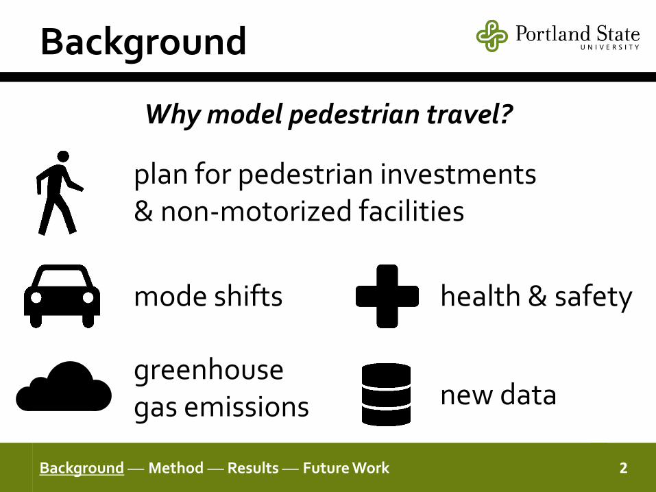
• Metro: metropolitan planning organization for Portland, OR
• Two research projects
Project overview
3Background — Method — Results — Future Work
travel demand estimation model
pedestrian demand estimation model
pedestrian scale
pedestrian environment
destination choice
mode choice
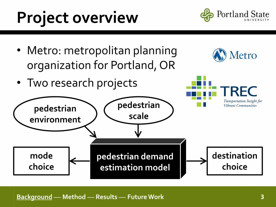
Current method
4
Trip Distribution or Destination Choice (TAZ)
Mode Choice (TAZ)
Trip Assignment
Pedestrian Trips
All Trips Pedestrian Trips Vehicular Trips
TAZ = transportation analysis zoneTrip Generation (TAZ)
Background — Method — Results — Future Work

New method
5
TAZ = transportation analysis zonePAZ = pedestrian analysis zone
Trip Generation (PAZ)
Trip Distribution or Destination Choice (TAZ)
Mode Choice (TAZ)
Trip AssignmentPedestrian Trips
Walk Mode Split (PAZ)
Destination Choice (PAZ)
I
II
All Trips Pedestrian Trips Vehicular Trips
Background — Method — Results — Future Work

Pedestrian analysis zones
6
TAZs PAZs
Home-based work trip productions
1/20 mile = 264 feet ≈ 1 minute walk
Metro: ~2,000 TAZs ~1.5 million PAZs
Background — Method — Results — Future Work

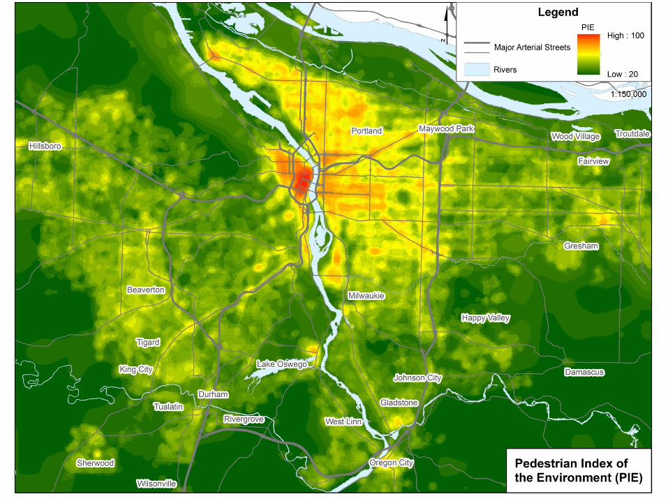
Pedestrian Index of the Environment (PIE)PIE is a 20–100 score total of 6 dimensions, calibrated to observed walking activity:
7
Pedestrian environment
People and job density
Transit access
Block size
Sidewalk extent
Comfortable facilities
Urban living infrastructure
Background — Method — Results — Future Work
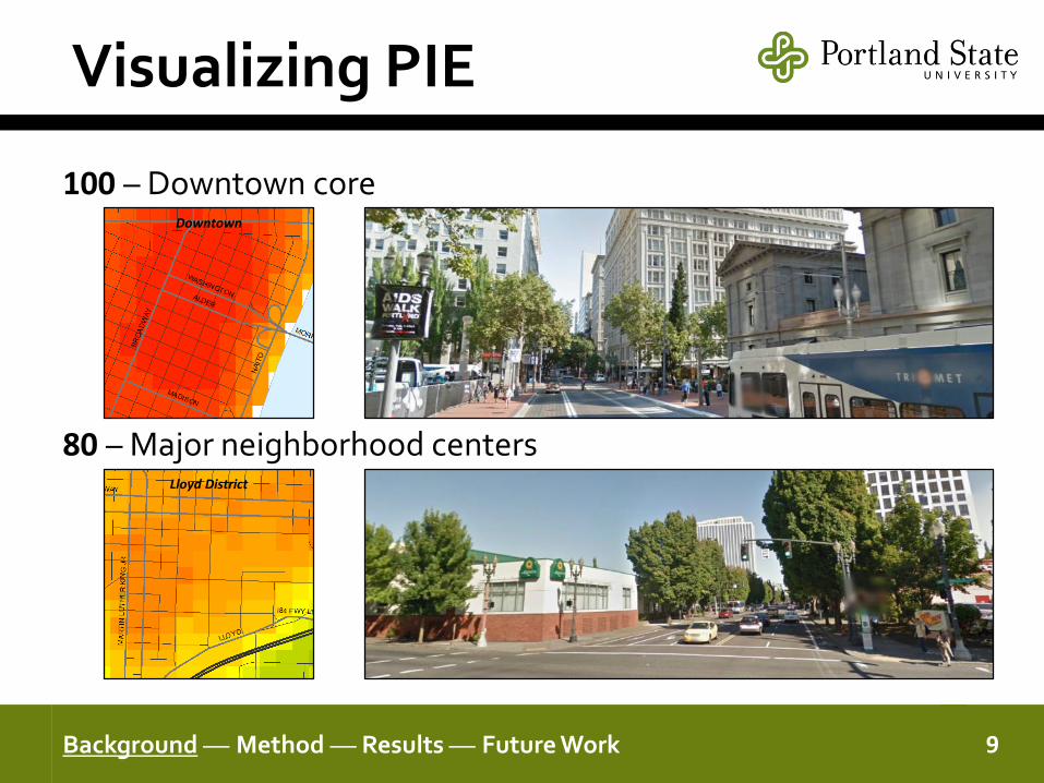
Visualizing PIE
9Background — Method — Results — Future Work
100 – Downtown core
80 – Major neighborhood centers
Downtown
Lloyd District
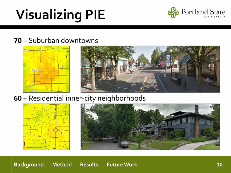
Visualizing PIE
10Background — Method — Results — Future Work
70 – Suburban downtowns
60 – Residential inner-city neighborhoods

Visualizing PIE
11Background — Method — Results — Future Work
50 – Suburban shopping malls
40 – Suburban neighborhoods/subdivisions
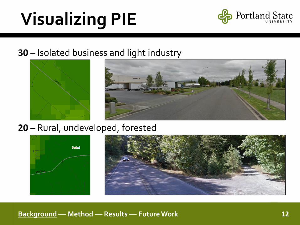
Visualizing PIE
12Background — Method — Results — Future Work
30 – Isolated business and light industry
20 – Rural, undeveloped, forested
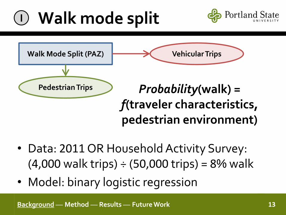
Walk mode split
Probability(walk) = f(traveler characteristics, pedestrian environment)
13
I
Walk Mode Split (PAZ)
Pedestrian Trips
Vehicular Trips
• Data: 2011 OR Household Activity Survey: (4,000 walk trips) ÷ (50,000 trips) = 8% walk
• Model: binary logistic regression
Background — Method — Results — Future Work
Walk Mode Split Results
Household characteristics
14
I
+ positively related to walking – negatively related to walking
number of children age of household
vehicle ownership
3.6%
4.4%
5.4%
0% 2% 4% 6%
Increase in odds of walking
home–work trips
home–other trips
other–other trips
Pedestrian environment+ positively related to walking
+ 1 point PIE
associated with:
Background — Method — Results — Future Work

Prob(dest.) = function of…– network distance– size ( # of destinations )– pedestrian environment– traveler characteristics
• Data: 2011 OHAS (4,000 walk trips)• Method: multinomial logit model
random sampling• Spatial unit: super-pedestrian analysis zone• Models estimated for 6 trip purposes
Destination choice
15
II
Background — Method — Results — Future Work
Pedestrian Trips
Destination Choice (PAZ)
16

17
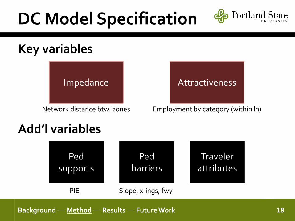
DC Model Specification
18Background — Method — Results — Future Work
Key variables
Impedance Attractiveness
Pedsupports
Pedbarriers
Traveler attributes
Add’l variables
Network distance btw. zones Employment by category (within ln)
PIE Slope, x-ings, fwy

Destination choice results
19Background — Method — Results — Future Work
HB Work
HB Shop
HB Rec
HB Other
NHBWork
NHB NW
Sample size 305 405 643 1,108 732 705
Pseudo R2 0.45 0.68 0.42 0.53 0.59 0.54
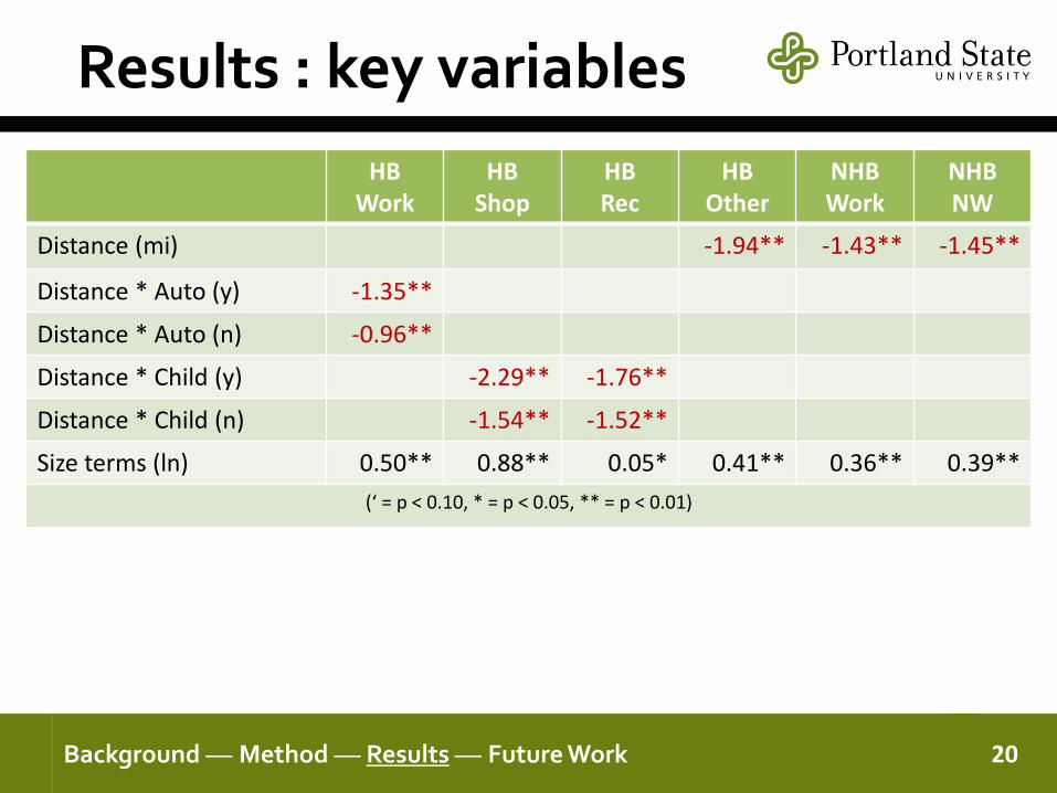
Results : key variables
20Background — Method — Results — Future Work
HBWork
HB Shop
HBRec
HBOther
NHBWork
NHBNW
Distance (mi) -1.94** -1.43** -1.45**
Distance * Auto (y) -1.35**
Distance * Auto (n) -0.96**
Distance * Child (y) -2.29** -1.76**
Distance * Child (n) -1.54** -1.52**
Size terms (ln) 0.50** 0.88** 0.05* 0.41** 0.36** 0.39**
(‘ = p < 0.10, * = p < 0.05, ** = p < 0.01)
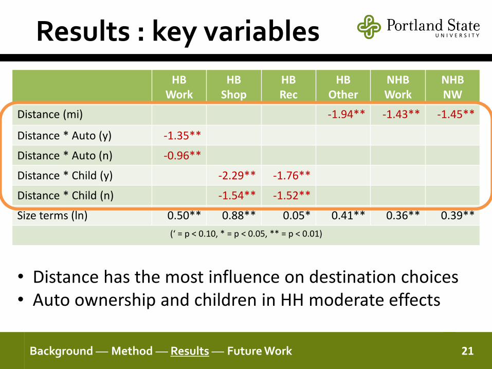
Results : key variables
21Background — Method — Results — Future Work
HBWork
HB Shop
HBRec
HBOther
NHBWork
NHBNW
Distance (mi) -1.94** -1.43** -1.45**
Distance * Auto (y) -1.35**
Distance * Auto (n) -0.96**
Distance * Child (y) -2.29** -1.76**
Distance * Child (n) -1.54** -1.52**
Size terms (ln) 0.50** 0.88** 0.05* 0.41** 0.36** 0.39**
(‘ = p < 0.10, * = p < 0.05, ** = p < 0.01)
• Distance has the most influence on destination choices• Auto ownership and children in HH moderate effects
Results : key variables
22Background — Method — Results — Future Work
HBWork
HB Shop
HBRec
HBOther
NHBWork
NHBNW
Distance (mi) -1.94** -1.43** -1.45**
Distance * Auto (y) -1.35**
Distance * Auto (n) -0.96**
Distance * Child (y) -2.29** -1.76**
Distance * Child (n) -1.54** -1.52**
Size terms (ln) 0.50** 0.88** 0.05* 0.41** 0.36** 0.39**
(‘ = p < 0.10, * = p < 0.05, ** = p < 0.01)
• No. of destinations inc. odds of choosing particular zone
• # Retail destinations dominates shopping purpose

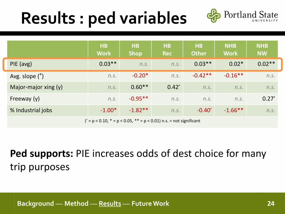
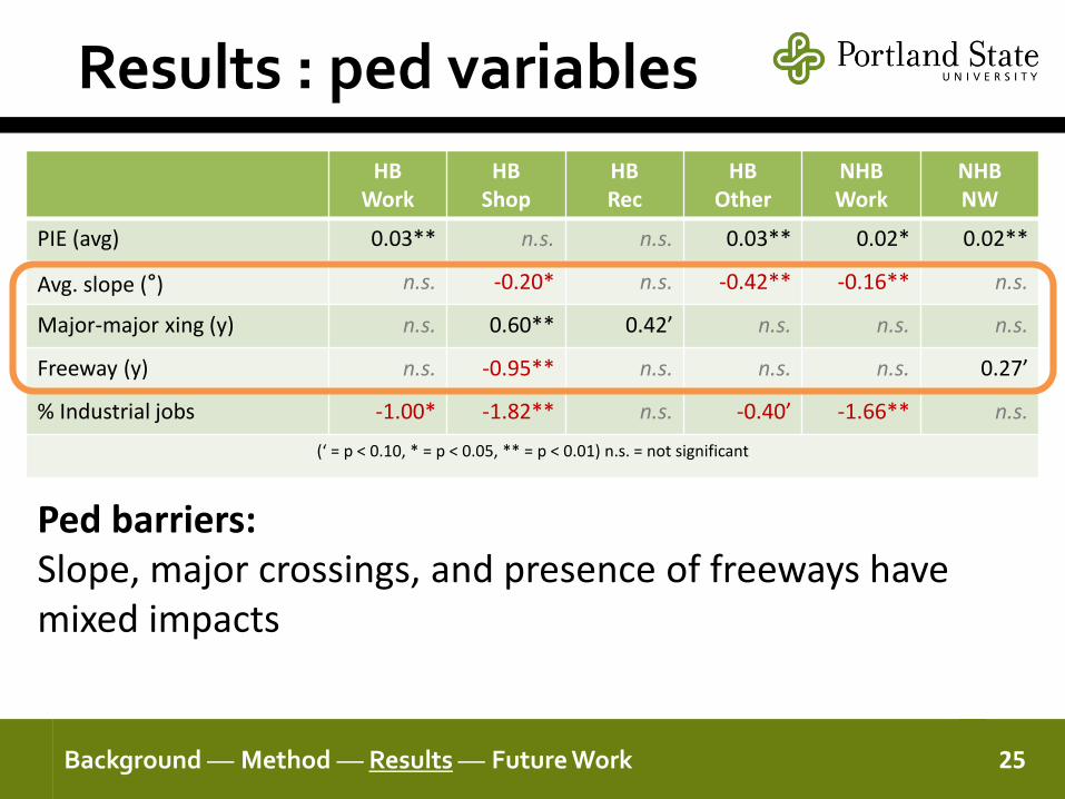
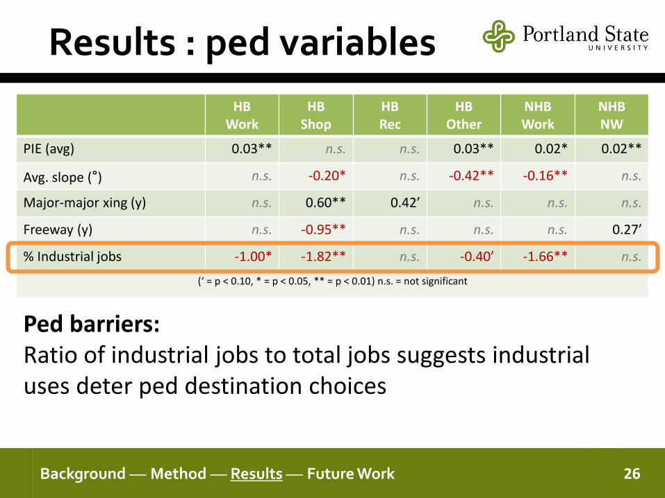
Results : ped variables
23Background — Method — Results — Future Work
HBWork
HBShop
HBRec
HBOther
NHBWork
NHBNW
PIE (avg) 0.03** n.s. n.s. 0.03** 0.02* 0.02**
Avg. slope (°) n.s. -0.20* n.s. -0.42** -0.16** n.s.
Major-major xing (y) n.s. 0.60** 0.42’ n.s. n.s. n.s.
Freeway (y) n.s. -0.95** n.s. n.s. n.s. 0.27’
% Industrial jobs -1.00* -1.82** n.s. -0.40’ -1.66** n.s.
(‘ = p < 0.10, * = p < 0.05, ** = p < 0.01) n.s. = not significant
Results : ped variables
24Background — Method — Results — Future Work
HBWork
HBShop
HBRec
HBOther
NHBWork
NHBNW
PIE (avg) 0.03** n.s. n.s. 0.03** 0.02* 0.02**
Avg. slope (°) n.s. -0.20* n.s. -0.42** -0.16** n.s.
Major-major xing (y) n.s. 0.60** 0.42’ n.s. n.s. n.s.
Freeway (y) n.s. -0.95** n.s. n.s. n.s. 0.27’
% Industrial jobs -1.00* -1.82** n.s. -0.40’ -1.66** n.s.
(‘ = p < 0.10, * = p < 0.05, ** = p < 0.01) n.s. = not significant
Ped supports: PIE increases odds of dest choice for many trip purposes
Results : ped variables
25Background — Method — Results — Future Work
HBWork
HBShop
HBRec
HBOther
NHBWork
NHBNW
PIE (avg) 0.03** n.s. n.s. 0.03** 0.02* 0.02**
Avg. slope (°) n.s. -0.20* n.s. -0.42** -0.16** n.s.
Major-major xing (y) n.s. 0.60** 0.42’ n.s. n.s. n.s.
Freeway (y) n.s. -0.95** n.s. n.s. n.s. 0.27’
% Industrial jobs -1.00* -1.82** n.s. -0.40’ -1.66** n.s.
(‘ = p < 0.10, * = p < 0.05, ** = p < 0.01) n.s. = not significant
Ped barriers: Slope, major crossings, and presence of freeways have mixed impacts
Results : ped variables
26Background — Method — Results — Future Work
HBWork
HBShop
HBRec
HBOther
NHBWork
NHBNW
PIE (avg) 0.03** n.s. n.s. 0.03** 0.02* 0.02**
Avg. slope (°) n.s. -0.20* n.s. -0.42** -0.16** n.s.
Major-major xing (y) n.s. 0.60** 0.42’ n.s. n.s. n.s.
Freeway (y) n.s. -0.95** n.s. n.s. n.s. 0.27’
% Industrial jobs -1.00* -1.82** n.s. -0.40’ -1.66** n.s.
(‘ = p < 0.10, * = p < 0.05, ** = p < 0.01) n.s. = not significant
Ped barriers: Ratio of industrial jobs to total jobs suggests industrial uses deter ped destination choices

Some Interpretation
27miles
0.14
0.17
0.19
0.00 0.25 0.50 0.75 1.00
HBO
NHBW
NHBNW
Equivalent distance reductions from 2 * (# destinations)
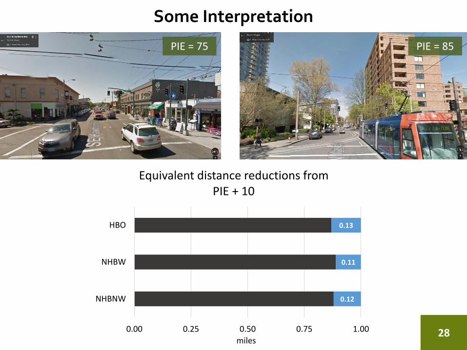
Some Interpretation
28
PIE = 75 PIE = 85
0.13
0.11
0.12
0.00 0.25 0.50 0.75 1.00
HBO
NHBW
NHBNW
Equivalent distance reductions from PIE + 10
miles
Conclusions
29Background — Method — Results — Future Work
• One of the first studies to examine destination choice of pedestrian trips
• Pedestrian scale analysis w/ pedestrian-relevant variables
• Distance and size have the most influence on ped. dest. choice
• Supports and barriers to walking also influence choice
• Traveler characteristics moderate distance effect

Future work
• Model improvements
– Choice set generation method & sample sizes
– Explore non-linear effects & other interactions
• Model validation & application
• Predict potential pedestrian paths
• Test method in other region(s)
• Incorporation into Metro trip-based model
30Background — Method — Results — Future Work

Questions?
Project report/info:http://otrec.us/project/510
http://otrec.us/project/677
Kelly J. Clifton, PhD [email protected]
Christopher D. Muhs [email protected]
Patrick A. Singleton [email protected]
Robert J. Schneider, PhD [email protected]
31
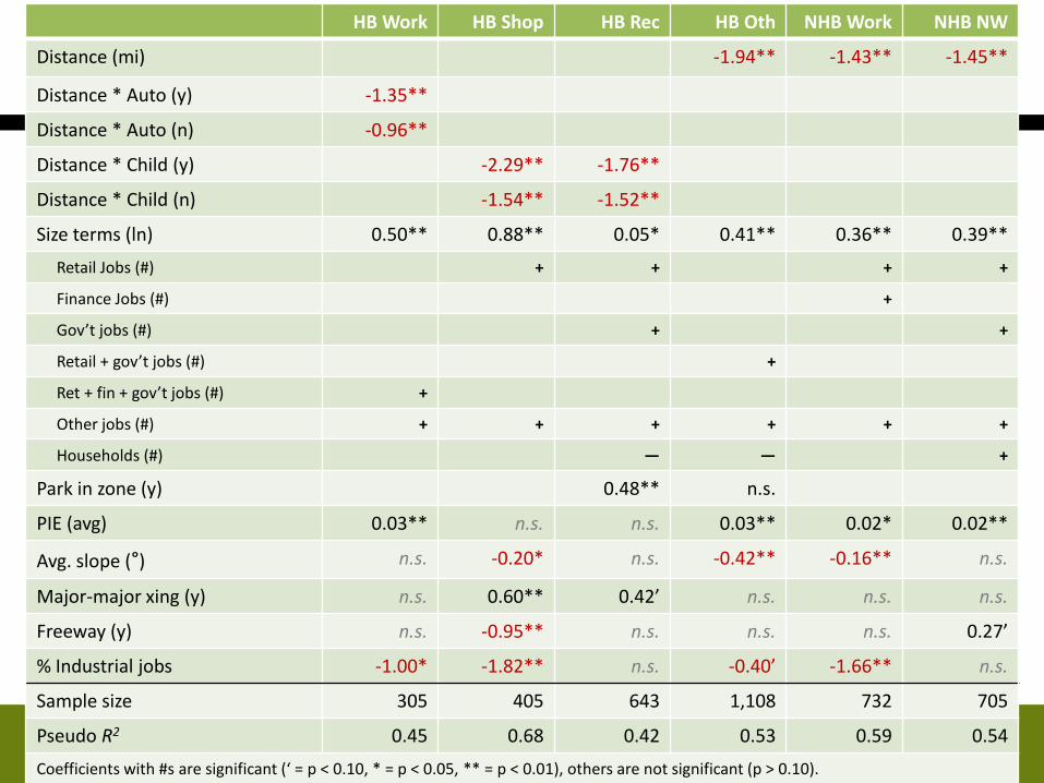
Destination choice results
32Background — Method — Results — Future Work
HB Work HB Shop HB Rec HB Oth NHB Work NHB NW
Distance (mi) -1.94** -1.43** -1.45**
Distance * Auto (y) -1.35**
Distance * Auto (n) -0.96**
Distance * Child (y) -2.29** -1.76**
Distance * Child (n) -1.54** -1.52**
Size terms (ln) 0.50** 0.88** 0.05* 0.41** 0.36** 0.39**
Retail Jobs (#) + + + +
Finance Jobs (#) +
Gov’t jobs (#) + +
Retail + gov’t jobs (#) +
Ret + fin + gov’t jobs (#) +
Other jobs (#) + + + + + +
Households (#) — — +
Park in zone (y) 0.48** n.s.
PIE (avg) 0.03** n.s. n.s. 0.03** 0.02* 0.02**
Avg. slope (°) n.s. -0.20* n.s. -0.42** -0.16** n.s.
Major-major xing (y) n.s. 0.60** 0.42’ n.s. n.s. n.s.
Freeway (y) n.s. -0.95** n.s. n.s. n.s. 0.27’
% Industrial jobs -1.00* -1.82** n.s. -0.40’ -1.66** n.s.
Sample size 305 405 643 1,108 732 705
Pseudo R2 0.45 0.68 0.42 0.53 0.59 0.54
Coefficients with #s are significant (‘ = p < 0.10, * = p < 0.05, ** = p < 0.01), others are not significant (p > 0.10).
Top Related