Estimation of pedestrian origin-destinationdemand in train stations

Flurin S. Hänseler� Nicholas A. Molyneaux�

Michel Bierlaire�

July 3, 2015

Report TRANSP-OR 150703Transport and Mobility Laboratory

School of Architecture, Civil and Environmental EngineeringEcole Polytechnique Fédérale de Lausanne

transp-or.epfl.ch

This is a revised version of technical report #150108.

�École Polytechnique Fédérale de Lausanne (EPFL), School of Architecture, Civil andEnvironmental Engineering (ENAC), Transport and Mobility Laboratory, Switzerland,{flurin.haenseler,nicholas.molyneaux,michel.bierlaire}@epfl.ch

1

We present a framework for estimating pedestrian demand within a trainstation. It takes into account ridership data, and various direct and indirectindicators of demand. Such indicators may include link flow counts, densitymeasurements, survey data, historical or other information. The problemis considered in discrete time and at the aggregate level, i.e., for groups ofpedestrians associated with the same origin-destination pair and departuretime interval. The formulation is probabilistic, allowing to consider thestochasticity of demand. A key element of the framework is the use of thetrain timetable to better capture demand peaks. A case study analysis ofa Swiss train station underlines its practical applicability. Compared to aclassical estimator that ignores the notion of a train timetable, the gain inaccuracy in terms of RMSE is between 20% and 50%. More importantly,the incorporation of the train schedule allows for prediction when littleor no data besides the timetable and ridership information is available.

Keywords: Origin-destination demand; schedule-based estimation; pedestrian

flows; public transportation.

1

1 Introduction

Pedestrian behavior in train stations increasingly attracts the attentionof academic research. Broadly, it can be distinguished between empiri-cal studies (Daly et al., 1991; Cheung and Lam, 1998; Pettersson, 2011;Ganansia et al., 2014), and those concerned with its modeling (Lee et al.,2001; Daamen, 2004; Kaakai et al., 2007; Xu et al., 2014). A review of theliterature is provided by Mustafa and Ashaari (2015).

Most studies make great efforts in describing behavioral aspects suchas walking, waiting or boarding. At the same time, only few methods areproposed in the literature to estimate pedestrian demand from data. Manystudies are solely based on theoretical demand scenarios (Hoogendoorn andDaamen, 2004; Rindsfüser and Klügl, 2007; Davidich et al., 2013). Otherstudies rely on simple assumptions to estimate demand (Kaakai et al., 2007;van den Heuvel and Hoogenraad, 2014), or consider railway stations thatserve only a single line (Lee et al., 2001; Xu et al., 2014). Yet knowledgeof pedestrian demand is a prerequisite for the analysis of pedestrian flowsin train stations, be it for the design of infrastructure, the optimizationof operations such as the train-track assignment, or real-time managementand control of pedestrian flows.

Several approaches to estimate pedestrian demand in train stations seemconceivable. For instance, an activity-based approach could be pursued(Danalet et al., 2014). However, for most train stations, disaggregate datais still unavailable, or only with low sampling rates and low temporal orspatial resolution. Instead, it is more efficient to estimate origin-destination(OD) demand at the aggregate level. Pedestrians may be divided into userclasses that are characterized by a common activity or behavior pattern,which in the context of a train station could be ‘inbound’, ‘outbound’, butalso ‘elderly’, ‘in a hurry’, or any combination thereof (Wong et al., 2005;Lavadinho, 2012).

The problem of estimating OD demand has a long history in the contextof road networks, for which link flow volumes and other indirect observa-tions of demand are available (van Zuylen and Willumsen, 1980; Cascetta,1984). Typically, an assignment map is assumed that relates observationsto OD volumes, such that the latter can be ‘reverse engineered’. This mapmay be obtained via a dynamic traffic assignment (DTA) model, combin-ing travel behavior models such as mode, departure time and route choice

2

models, as well as a network loading model. In the context of pedestrianflows in train stations, mode choice is irrelevant, and the choice of departuretime is mainly governed by the train timetable, which is discussed in thiswork. A variety of approaches have been proposed for route choice (Cheungand Lam, 1998; Hoogendoorn and Bovy, 2004; Daamen et al., 2005), andfor network loading models a rich literature is available as well (Lee et al.,2001; Daamen, 2004; Kaakai et al., 2007; Xu et al., 2014; Starmans et al.,2014). The problem of pedestrian OD demand estimation in train stationsis thus in principle amenable to ‘classical’ estimation techniques.

A key issue in OD demand estimation is the ratio between the num-ber of unknowns and the number of independent observations, yielding anintrinsically underdetermined problem. Various forms of exogenous infor-mation, either in the form of a priori knowledge or structural assumptions,are used to lead the calculation to a unique solution.

For static OD estimation, concepts like gravity (Casey, 1955), entropymaximization (Wilson, 1970; Willumsen, 1981) or information minimiza-tion (van Zuylen and Willumsen, 1980) have been used. In most cases,however, an a priori OD trip table (Cascetta and Nguyen, 1988) is used.Other researchers make specific assumptions on the structure of OD triptables (Bierlaire and Toint, 1995) or the covariance across measurements(Hazelton, 2003).

For dynamic problems, a common approach is to assume a dynamicprocess for the evolution of demand, such as an autoregressive process inthe deviates from historical estimates (Ashok and Ben-Akiva, 2000; Bier-laire and Crittin, 2004; Zhou and Mahmassani, 2007). Recent approachesassume slowly evolving route split fractions in the framework of a ‘quasi-dynamic’ estimator (Marzano et al., 2009; Cascetta et al., 2013), or reducethe dimensionality of the estimation problem by applying principal com-ponent analysis (Djukic et al., 2012).

Several researchers consider also the problem of OD demand estimationin transit networks. Early approaches assume a constant average cost alongroutes (Nguyen et al., 1988), whereas newer studies focus on schedule-basedtransit network models (Wong and Tong, 1998), of which some additionallyconsider passenger overload delays (Lam et al., 2003) or data from ICTsensors (Montero et al., 2015). These models can predict the evolution ofin- and outflows at stations or the number of passengers in vehicles, but donot provide detailed information on OD demand within a train station.

3

Pedestrian OD demand in train stations is particularly unsteady due toarriving and departing trains that lead to demand ‘micro-patterns’. More-over, acyclic schedules and unplanned delays make it difficult to use his-torical OD data, or any other of the aforementioned approaches for dealingwith underdetermination. This is where we would like to make a contri-bution. In this paper, we propose a dedicated methodology for estimatingpedestrian OD demand in train stations in general, and we do so by ex-plicitly integrating the train timetable and ridership data in particular.

2 Data sources

To reduce the underdetermination, the use of any relevant, available datais desirable. In comparison to motorized traffic, there are several inherentchallenges that make the monitoring of pedestrian traffic difficult. First,pedestrians are not confined to fixed lanes, and can explore space freely.This makes the placement of sensors difficult, and may decrease their ac-curacy. Second, pedestrians often travel in groups. Special care must betaken to differentiate between individuals, and to take into account effectssuch as occlusion (Alahi et al., 2014). Third, pedestrian traffic is typicallymore variable than motorized traffic, implying that sensors are required tocapture a large range of traffic levels (cf. Traffic Monitoring Guide, U.S.Department of Transportation, 2013).

In the following, five types of data sources are discussed that are rele-vant for the case of a train station. For a discussion of sensing technolo-gies, including guidance on making the most appropriate choice for selectedpractical applications, we refer instead to Turner et al. (2007), Bauer et al.(2009) and the aforementioned Traffic Monitoring Guide (U.S. Departmentof Transportation, 2013).

OD flow data: OD flow data represent direct observations of OD demandthat are obtained from surveys, pedestrian tracking systems, or ICT sensors(e.g. Bluetooth and WiFi scanners for smartphones). Such observations aregenerally expensive to collect and rare (Bauer et al., 2009).

Automatic collection techniques depend on the location of sensors, andtheir sampling rate. Typically, they do not cover the entire network ofinterest. Also, if only a subset of pedestrians is detected, this needs to

4

be corrected by means of sampling rates. Their estimation is difficult, asthey are generally time- and location-dependent (Bauer et al., 2009). Thereexist two ways to deal with that. Either the sampling rates are estimateda priori, or directly within the OD estimation process. While the latter istheoretically more attractive due to its generality, it is also computationallymore expensive.

Link flow data: In analogy to car traffic, a pedestrian facility may bethought of as a network of links. Links denote walkways or walkway sec-tions, such as a part of a corridor, stairway, or an escalator. On links, flowscan be observed at a physical gate, such as a turnstile or a train door, orat a virtual gate like the entrance of a walkway. Link flow data representindirect observations of OD demand, and depend on route choice decisionsand prevailing traffic conditions.

Link flow data are typically more accurate than OD flow data, but sam-pling may still be an issue, especially for camera-based detectors (Ganansiaet al., 2014). The number and position of detectors plays a crucial role forthe observability of OD demand (Gentili and Mirchandani, 2012; Yang andFan, 2015). Ideally, if a link exclusively serves routes associated with asingle OD pair, a well-placed detector may be used to directly infer theOD volumes for that particular OD pair. Also, if detectors are located onlinks that are adjacent to origin and destination nodes, they may providean estimate of the generation of that node. On the other hand, if measure-ments are highly correlated, further sensors may not provide substantialadditional information.

Other traffic condition data: Other traffic condition data include den-sities, walking speeds and point-to-point travel times. They characterizethe system response of the traffic network to a given OD demand.

Such data may be obtained from pedestrian tracking systems or ICTsensors. Speed or density measurements can for instance help to identifywhether a link is in a congested or uncongested state, and thus to adjustthe OD demand in one way or another (Djukic et al., 2015). There existseveral ways of including this type of input data in the estimation process.One is to include it in the objective function of the estimation problem.A DTA model is then used to define the relationship between OD demandand traffic conditions, and a match between observation and estimation

5

is sought. Alternatively, traffic condition data may be used to replace theDTA model altogether. For instance, Montero et al. (2015) use travel timescollected from ICT sensors to estimate the travel time distributions. Theseare then used as time-varying exogenous model parameters.

Train timetable and ridership data: Pedestrian demand within a trainstation and the train timetable are inextricably intertwined. To establisha formal relationship between the two, the train-track assignment and thetrain exchange volumes are useful, i.e., the number of boarding and alight-ing passengers for each train.

Unplanned changes in the train timetable and train-track assignmentare common in most railway systems around the world (Higgins and Kozan,1998; Cule et al., 2011). For highly inter-connected timetables or denserailway traffic, a single delayed train may cause a domino effect of secondarydelays due to infrastructure restrictions, connection constraints or logistics.Several approaches are available to predict the actual timetable based onthe scheduled one (Goverde, 2007; Yuan and Hansen, 2007).

The train exchange volumes may be inferred from traffic surveys, ticketsales, or train capacities. Additionally, some trains are equipped with doorcounters that not only allow for an automatic detection of these volumes,but also for an estimation of their distribution across vehicles. Especiallyon long platforms, such distributional information can be important for anaccurate understanding of the usage of a train station.

Other data: Further data sources can be useful to narrow the solutionspace. Such information typically comes in the form of survey data. Inmany train stations, service and sales points are found. The number ofcustomer visits to these places may be known, and can be used as an apriori estimate of the corresponding origin or destination flows. Similarly,railway operators often have an idea of the relative share of certain userclasses, such as transfer passengers. This information may be used in theform of destination split ratios.

6

3 Methodological framework

This section presents a methodological framework for estimating pedestrianOD demand based on the notion of a train timetable, and an exemplaryspecification that is applicable to any suitable train station. Section 4 thenpresents a case study based on that specification.

3.1 Notation

A recapitulation of important variables is provided in Appendix A.

3.1.1 Time and space representation

The time period of interest is divided into a set of discrete intervals T ,where each interval τ ∈ T is of uniform length ∆t.

Walkable space is represented by a directed graph G = (N ,L), whereN is the set of nodes ν ∈ N , and L the set of directed links λ ∈ L. Cer-tain elements of pedestrian facilities, such as stairs or corridors, translatenaturally into links, and others naturally into nodes, like for instance ODareas. For other elements, such as waiting halls or platforms, a decompo-sition into areas can be made. An area α is associated with a subnetwork(Nα,Lα) denoted by Gα. The set Nα contains all the nodes correspondingto physical locations in the area, and Lα ⊂ L all links such that their twoincident nodes belong to Nα. Areas are allowed to overlap, and their unionis not required to cover the full network.

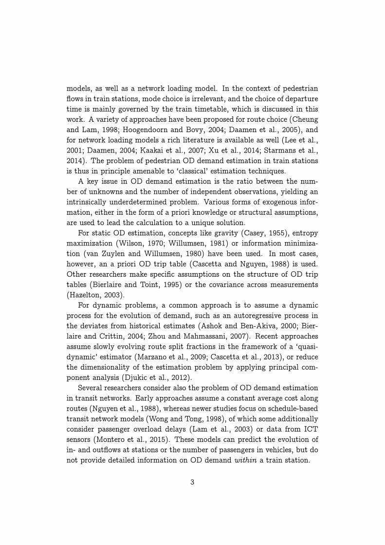
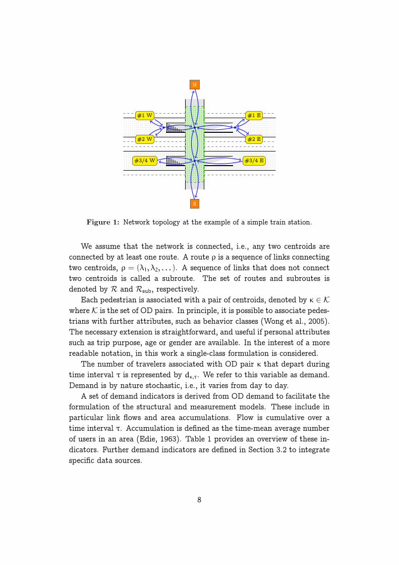
Fig. 1 illustrates the proposed space representation. Railway tracks aredenoted by dotted lines. Levels are bridged by ramps and stairways, de-noted by standard floor plan symbols. Platform sectors are represented bycentroids shown as rectangles with rounded corners. They may be associ-ated with one or a pair of railway tracks. Further centroids are shown assquares, which include sales or service points, or exit/entrance areas. Thepedestrian walking network is represented by solid lines. An exemplaryarea is shaded.

3.1.2 Demand representation

Nodes through which pedestrians enter and leave the pedestrian networkare referred to as centroids, and their set is denoted by C ⊂ N .

7

#1 W

#2 W

#1 E

#2 E

#3/4 W #3/4 E

N

S

Figure 1: Network topology at the example of a simple train station.

We assume that the network is connected, i.e., any two centroids areconnected by at least one route. A route ρ is a sequence of links connectingtwo centroids, ρ = (λ1, λ2, . . . ). A sequence of links that does not connecttwo centroids is called a subroute. The set of routes and subroutes isdenoted by R and Rsub, respectively.

Each pedestrian is associated with a pair of centroids, denoted by κ ∈ K

where K is the set of OD pairs. In principle, it is possible to associate pedes-trians with further attributes, such as behavior classes (Wong et al., 2005).The necessary extension is straightforward, and useful if personal attributessuch as trip purpose, age or gender are available. In the interest of a morereadable notation, in this work a single-class formulation is considered.

The number of travelers associated with OD pair κ that depart duringtime interval τ is represented by dκ,τ. We refer to this variable as demand.Demand is by nature stochastic, i.e., it varies from day to day.

A set of demand indicators is derived from OD demand to facilitate theformulation of the structural and measurement models. These include inparticular link flows and area accumulations. Flow is cumulative over atime interval τ. Accumulation is defined as the time-mean average numberof users in an area (Edie, 1963). Table 1 provides an overview of these in-dicators. Further demand indicators are defined in Section 3.2 to integratespecific data sources.

8

Table 1: List of demand and demand indicators. The unit is ‘number of pedes-trians per unit of time’, unless stated otherwise.

d = [dκ,τ] Demand dκ,τ associated with OD pair κ and departure time interval τ,and time-space expanded vector d of length |K||T |.

f = [fλ,τ] Flow fλ,τ entering link λ during time interval τ, and time-space ex-panded vector f of length |L||T |.

a = [aα,τ] Time-mean average accumulation aα,τ on area α during time intervalτ, and time-space expanded vector a of length |A||T |.

eoff = [eoffζ ],eon = [eonζ ]

Train exchange volumes associated with alighting, eoffζ , and boarding,eonζ , of train ζ, and corresponding vectors eoff and eon of length |K|.The unit is ‘number of pedestrians’.

3.1.3 Representation of trains

A set of trains Z is considered. For a train ζ ∈ Z, tarrζ and tdepζ denote the

actual arrival and departure time in the train station. They are assumed tofollow a known random distribution that may be obtained empirically, orfrom any suitable delay model. Each train is associated with an alightingand boarding volume, referred to as train exchange volumes and denotedby eoff

ζ and eonζ , respectively. The platform serving train ζ is denoted by πζ.

Each platform π ∈ P, with P the set of all platforms, is associated with aset of centroids, Cπ ⊂ C.

3.2 Data requirements

To distinguish between model estimates and actual observations, ‘biased’variables such as measurements are marked by a hat (e.g. f). Often, suchobservations are not available for the complete network, or only for certaintime intervals. Vectors containing a reduced set of variables are marked bya prime (e.g. f ′), and a reduction matrix ∆ is defined that relates each ofthem to the corresponding full vector (e.g. f ′ = ∆ff).

For the estimation methodology, availability of the actual train timetable,tarrζ and tdep

ζ for each train ζ ∈ Z, and of the corresponding exchangevolumes eoff

ζ , eonζ is essential. Moreover, partial indirect observations of de-

mand, for instance in the form of link flows f ′ or area accumulations a′, arerequired. These observations need to be such that demand micro-patternsof individual trains are captured, i.e., an aggregation in the order of min-

9

utes is desirable. Availability of an a priori estimate of demand d′ is usefulto improve the estimation, but not mandatory.

Example specification: To illustrate the demand estimation method-ology, a concrete specification is elaborated. For that purpose, severalassumptions are made throughout the document. The general estimationmethodology is independent of these assumptions.

Assumption 1 (Data availability) Available are (i) the actual train

timetable, (ii) train exchange volumes, (iii) partial observations of link

flows, (iv) aggregate destination split ratios (e.g. from travel surveys),

and (v) cumulative origin and destination flows for selected centroids

(e.g. from sales data). For validation, (vi) partial observations of area

accumulations, and (vii) flows along selected subroutes are available.

No historical demand prior is considered.

To capture the format of these data sources, additional demand indica-tors are defined in Table 2.

Table 2: Additional demand indicators.

fsub = [fsub,τ ] Subroute flow esub

,τ reaching subroute during time interval τ,and time-space expanded vector fsub of length |Rsub||T |. Itsunit is ‘number of pedestrians per unit time’.

fout,cum = [fout,cumν ] Cumulative origin flow fout,cum

ν emanating from centroid ν dur-ing the time period T , and vector fout,cum of length |C|. Itsunit is ‘number of pedestrians’.

fin,cum = [fin,cumν ] Cumulative destination flow fin,cum

ν reaching centroid ν duringtime period T , and vector fin,cum of length |C|. Its unit is‘number of pedestrians’.

ravg = [ravgν ] Time-mean average ratio ravg

ν of users headed for a platformin the origin flow at centroid ν during time period T , andvector ravg of length |C|. The destination split ratio ravg

ν isdimensionless.

3.3 Structural model

The structural model describes the relationship among the various variablesinvolved in the framework. We consider two parts, namely an assignment

10

model, and a schedule-based model that considers the arrivals and depar-tures of trains.

3.3.1 Assignment model

A pre-specified aggregate network supply model, referred to as assignmentmodel, is assumed to exist. It is designed to derive the demand indicatorsfrom a given demand, depending on a parameter vector y. If Σ(d;y) de-notes the assignment model, and if Σ(·) is its output with respect to demandindicator (·) and η(·) the corresponding structural error, the aforementioneddemand indicators may be expressed as

f = Σf(d;y) + ηf, (1)

a = Σa(d;y) + ηa. (2)

In this work, we assume the vector y to be known a priori, but note thatit could also be estimated simultaneously with demand. Such an approachincurs substantial computational cost, and is not commonly pursued in theliterature (Cascetta and Improta, 2002).

To implement Eq. (1) and Eq. (2), any suitable supply model may beused. It can be a simple linear mapping, or a detailed commercial DTAmodel such as PTV Viswalk or Legion for Aimsun. Essential is that basicsupply variables like flow and density are provided. Additional informationsuch as user class-specific properties or walking speeds may be useful toimprove the estimation.

Internally, most assignment models perform two steps to obtain an es-timate of demand indicators. First, OD demand is mapped to route flowsby means of a route choice model. For a given OD pair and known link androute attributes, it identifies the route that a traveler would select. Thechoice of alternatives, and all attributes are assumed to be known. A largenumber of route choice models are available for that purpose (see e.g. Dial,1971; Cascetta et al., 1996; Ben-Akiva and Bierlaire, 2003; Frejinger andBierlaire, 2007). Second, a network loading model is used to describe thepropagation of pedestrians along the routes. A large number of models isavailable in the literature as well (e.g. Løvås, 1994; Helbing and Molnár,1995; Blue and Adler, 2001; Hughes, 2002; Antonini et al., 2006; Hänseleret al., 2014). To represent heterogeneity among pedestrians, route choice

11

and network loading are usually expressed by means of probability distri-butions.

Both route choice and network loading are subject to prevailing trafficconditions, and thus mutually dependent. If the dependency on prevailingtraffic conditions is neglected, the relationship between demand and de-rived indicators becomes linear (Cascetta and Improta, 2002). This holdstrue for an uncongested network. Alternatively, if the traffic situation isknown a priori through direct measurements, an estimate of the assign-ment maps may also be obtained without considering the demand (see theaforementioned example by Montero et al., 2015).

If on the other hand a network is congested and link travel times areunknown, a problem of circular dependence arises between the demandestimation and the network supply model. One way of dealing with thatis by formulating a bi-level optimization problem that explicitly includestraffic equilibrium conditions. Among the most popular studies pursuingsuch an approach are those by Fisk (1988), Yang (1995) and Florian andChen (1995). An alternative way to consider the mutual dependency be-tween the demand and supply model is by using a fixed-point formulation(Cascetta and Postorino, 2001; Bierlaire and Crittin, 2006).

Example specification: An assignment model for pedestrian walkingfacilities in a train station with a low level of congestion is considered.It consists of two independent models for route choice and network load-ing. For the sake of simplicity, we consider an assignment that is demand-independent.

Following Dial (1971), we adapt a probabilistic route choice model thatis suitable for traffic assignment and behaviorally accurate in the contextof pedestrian flows (Bierlaire and Robin, 2009).

Assumption 2 (Route choice) The route choice decision rule is given

by a logit model, where the cost of a route is equal to the sum of link

traversal times. The set of routes is finite and known.

Following Mustafa and Ashaari (2015), we assume that walking speedin pedestrian facilities of a train station with a low or medium level ofcongestion is normally distributed (LOS E or better, Highway CapacityManual, 2000, Exhibit 18-3).

12

Assumption 3 (Network loading) The propagation of pedestrians along

routes is described by a demand-invariant walking speed distribution

fv(v). The corresponding cumulative distribution function is denoted

by Fv(v).

The resulting mathematical specification of the assignment model isprovided in Appendix B.

3.3.2 Schedule-based model

The schedule-based model establishes a relationship between OD demandand train exchange volumes. It is based on the assumption that the alight-ing volume of trains served by a specific platform is related to the demandemanating from centroids representing that platform, and vice versa forboarding volumes.

Pedestrian demand within a train station is associated with alightingvolumes by an assignment matrix H = [hζ,(κ,τ)] and a corresponding errorεoff such that

eoff = Hd+ εoff. (3)

The error εoff takes into account pedestrians that visit a platform bymistake, or e.g. to accompany a passenger. The entry hζ,(κ,τ) represents theproportion of pedestrians associated with OD pair κ and departure timeinterval τ that have alighted from train ζ. It is high if the time interval

τ coincides with the idling time[

tarrζ , tdepζ

]

of train ζ on platform π, and

if the origin node νoκ of OD pair κ is associated with the correspondingplatform, i.e., if νoκ ∈ Cπ. Otherwise, it is zero. Under the basic assumptionthat demand is distributed homogeneously within a demand interval, theentries of the assignment matrix H are given by

hζ,(κ,τ) =

∣

∣

∣

[

tarrζ , tdepζ

]

∩ τ∣

∣

∣/|τ| if νoκ ∈ Cπ,

0 otherwise,(4)

where |τ′| represents the length of time interval τ′.In principle, a similar approach may be used to relate OD demand to

boarding volumes. However, it is difficult to find a meaningful specifica-tion of the corresponding assignment matrix. Prospective passengers oftenarrive at the platform long before the scheduled departure, which may be

13

due to constraints imposed by the schedule of tertiary transport modes, ora high risk aversion (van Hagen, 2011). We leave the development of anappropriate arrival process, for instance based on a Poisson distribution,for future research.

For now, boarding volumes may be considered in a temporally aggre-gated way. We denote by fdep,cum

π the cumulative departure flow from plat-form π during time period T , given by

fdep,cumπ =

∑

τ∈T

∑

ν∈Cπ

∑

κ∈Kdestν

dκ,τ∆t, (5)

where the set Kdestν contains all OD pairs with destination ν. The corre-

sponding vector fdep,cum = [fdep,cumπ ] is of length |P|.

If εχ represents a vector containing structural errors, the vector of cu-mulative platform departure flows can also be expressed by summing overthe boarding volumes of the served trains, i.e.,

fdep,cum = χ(eon) + εχ, (6)

where χ = [χπ] is given by

χπ(eon) =∑

ζ∈Zπ

eonζ , (7)

and where Zπ is the set of trains associated with platform π.Eq. (6) provides no information about the distribution of demand across

time. Similarly, Eq. (3) may not provide significant temporal informationunless the train idling times are of approximately the same length as thediscretization time intervals.

Empirical relations between OD demand and exchange volumes mayinstead be used to obtain such temporal information. This approach isillustrated at the example of ‘train-induced arrival flows’, and further dis-cussed in the specification below.

We assume there exists an empirical model that predicts the flow onplatform exit ways caused by pedestrians that have alighted from a train.

Let Larrπ denote the set of links representing the exit ways of platform

π, and φλ,τ(eoff;y) a model that predicts the cumulative flow on link λ ∈

LarrP during time interval τ based on the arrival times of trains and their

alighting volumes. If ϕ(eoff;y) = [φλ,τ] represents the corresponding time-space expanded vector, it holds that

farr = ϕ(eoff;y) + εϕ, (8)

14

where εϕ denotes a structural error, and where the flow vector associatedwith arrival links is given by

farr = ∆arrf (9)

and where the reduction matrix ∆arr is of size |LarrP ||T | × |L||T |.

Eq. (8) can be used to merely complement, or to replace Eq. (3). Ifan accurate empirical model is available, Eq. (3) does not provide muchadditional information, and can be omitted. This is assumed to be thecase in the specification below. If on the other hand both Eq. (3) andEq. (8) are used, a strong correlation among their error terms is likely toexist and needs to be explicitly considered.

Example specification: Our approach is inspired by Benmoussa et al.(2011) and Lavadinho (2012).

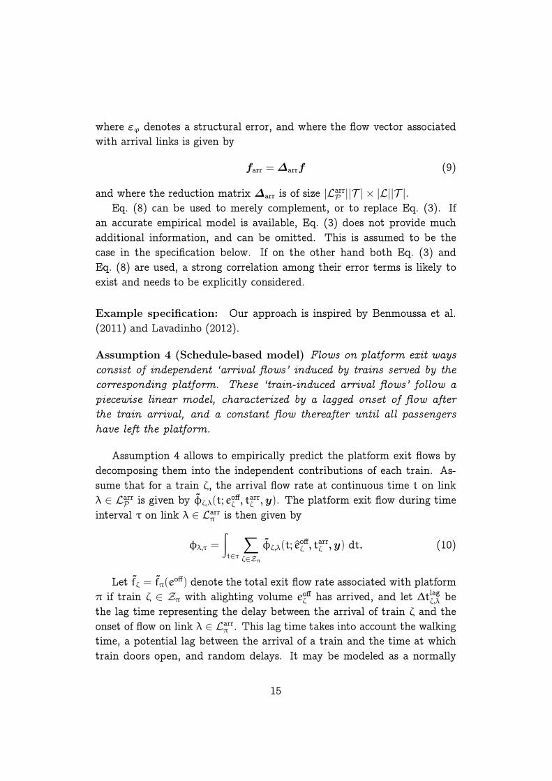
Assumption 4 (Schedule-based model) Flows on platform exit ways

consist of independent ‘arrival flows’ induced by trains served by the

corresponding platform. These ‘train-induced arrival flows’ follow a

piecewise linear model, characterized by a lagged onset of flow after

the train arrival, and a constant flow thereafter until all passengers

have left the platform.

Assumption 4 allows to empirically predict the platform exit flows bydecomposing them into the independent contributions of each train. As-sume that for a train ζ, the arrival flow rate at continuous time t on linkλ ∈ Larr

P is given by φζ,λ(t; eoffζ , t

arrζ ,y). The platform exit flow during time

interval τ on link λ ∈ Larrπ is then given by

φλ,τ =

∫

t∈τ

∑

ζ∈Zπ

φζ,λ(t; eoffζ , t

arrζ ,y) dt. (10)

Let fζ = fπ(eoff) denote the total exit flow rate associated with platformπ if train ζ ∈ Zπ with alighting volume eoff

ζ has arrived, and let ∆tlagζ,λ bethe lag time representing the delay between the arrival of train ζ and theonset of flow on link λ ∈ Larr

π . This lag time takes into account the walkingtime, a potential lag between the arrival of a train and the time at whichtrain doors open, and random delays. It may be modeled as a normally

15

distributed random variable, and assumed to depend on the platform only,i.e., ∆tlagζ,λ = ∆t

lagπ , where π = πζ (Molyneaux et al., 2014).

Assuming that the total exit flow rate of platform π is shared accordingto platform sector split fractions rsecζ,λ with

∑λ∈Larr

πrsecζ,λ = 1, the flow rate on

link λ associated with train ζ ∈ Zπ is given by

φζ,λ(t) =

rsecζ,λ fζ t ∈(

tarrζ + ∆tlagζ,λ, tarrζ + ∆tlagζ,λ + e

offζ /fζ

)

,

0 otherwise.(11)

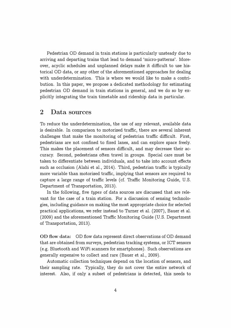
Fig. 2 illustrates the cumulative arrival flow associated with Eq. (11).The solid curve illustrates an observation from Lausanne railway station(Molyneaux et al., 2014), and the dash-dotted curve a piecewise linear ap-proximation.

time

cum

ula

tive

arri

vals

typical observationmodel

rsecζ,λeoffζ

∆tlagζ,λ

eoffζ /fζ

tarrζ

rsecζ,λfζ

Figure 2: Model for train-induced arrival flows.

The total platform exit flow rate fπ(eoff) is assumed to depend linearlyon the alighting volume eoff at low values, and to reach saturation at aplatform-specific threshold ecrit

π . If qπ, bπ and cπ represent shape parame-ters, the total exit flow rate on platform π is given by the stochastic model

fπ(eoff) = fdet

π (eoff) +N (0, qπ), (12)

where the deterministic part of the flow rate is specified as

fdetπ (eoff) =

{bπe

off + cπ if eoff ≤ ecritπ ,

bπecritπ + cπ otherwise.

(13)

16

Eq. (11) and Eq. (12) may be specified based on studies by Weidmann(1992), Buchmüller and Weidmann (2008) and Molyneaux et al. (2014).Alternatively, they can be calibrated on actual data. An example of thelatter is provided in Section 4.

3.4 Measurement model

The measurement model links the structural model to a priori informationand measurements, which are useful for the estimation of demand, and forvalidating the obtained results.

For each data source, a random error term takes into account the un-certainty it is afflicted with, and the aforementioned reduction matricesaccount for the incomplete coverage of the data collection infrastructure,i.e.,

d′ = ∆dd+ ω′d, (14)

f ′ = ∆ff + ω′f, (15)

a′ = ∆aa+ ω′a, (16)

e′on = ∆oneon + ω′

on, (17)

e′off = ∆offeoff + ω′

off. (18)

The measurement errors ω(·) are generally correlated, both across timeand space. Temporal correlation occurs if a sensor is malfunctioning, or ifit reaches saturation. Spatial correlation is a concern if two sensors capturesimilar information, for instance if they are placed nearby. For an efficientstatistical inference, these effects need to be taken into account by usingan appropriate covariance matrix.

Example specification: For the illustration of the model, the estimationproblem is reduced to a formulation that is linear in the unknown demandvector.

The cumulative origin and destination flows as well as the destination

17

split fractions are obtained by aggregation, i.e.,

fout,cumν =

∑

τ∈T

∑

κ∈Korigν

dκ,τ∆t, (19)

fin,cumν =

∑

τ∈T

∑

κ∈Kdestν

dκ,τ∆t, (20)

ravgν =

∑

τ∈T

∑

κ∈Korigν , νdκ∈CP

dκ,τ∆t/fout,cumν , (21)

where νdκ is the destination of OD pair κ, and where Korigν and Kdest

ν denotethe set of OD pairs which originate and terminate in centroid ν, respec-tively.

Assumption 5 (Measurement model) The distribution of train ex-

change volumes is a priori known, and used to pre-compute cumulative

platform departure as well as platform arrival flows.

The measurement model is given by Eq. (15), as well as by

f ′out,cum = ∆outfout,cum + ω′

out, (22)

f ′in,cum = ∆infin,cum + ω′

in, (23)

r′avg = ∆rravg + ω′

r. (24)

ϕ = ∆arrf + ωϕ, (25)

χ = fdep,cum + ωχ. (26)

Eq. (25) and Eq. (26) consider empirical estimates of platform arrival anddeparture flows, ϕ and χ, which are pre-computed based on the traintimetable and a priori known train exchange volumes. This pre-processingis useful to simplify the solution of the example specification, but not anecessity of the framework.

3.5 Estimation problem

The estimation problem consists in finding the distribution of the OD de-mand volumes d⋆ such that (i) actual observations of demand indicators arereproduced at best, (ii) platform arrival and platform departure flows are‘most consistent’ with empirical predictions based on the train timetable,

18

and (iii) the resulting estimate matches the historical one in case the esti-mation problem is underdetermined.

In the most general case, these three objectives are captured by a jointdistance measure dist〈·〉. A statistically meaningful specification can befound using pure likelihood methods, or within the Bayesian framework,and depends on the assumptions that are made regarding the distributionof the error terms (Hazelton, 2000).

Alternatively, if the cross-correlation across the three objectives is neg-ligible, the joint distance measure can be replaced by three separate termsdistobs〈·〉, distsched〈·〉 and disthist〈·〉. The estimation problem reads then as

d⋆

y = arg mind≥0

distobs

⟨

e′on

e′off

f ′

a′

,

e′on

e′off

f ′

a′

⟩

+distsched

⟨(

ϕ′

χ′

)

,

(

f ′arr

f ′dep,cum

)⟩

+disthist

⟨

d′,d′⟩

.

(27)While the distance measures in Eq. (27) are mutually independent, inter-nally they may still consider complex error structures that, for instance inthe context of least squares, can be taken into account by inner weights.

When solving Eq. (27), it is critical not to rely on point estimates. Thedemand vector d⋆ is generally distributed, and follows a complex distri-bution that is insufficiently described by a single value such as its mean.The distribution depends both on the variation of input variables, whichcan be distributed themselves, and on the uncertainty involved in terms ofmodeling and measurement errors.

To approximate the distribution of d⋆, Monte Carlo sampling may beused. Demand on each day is assumed to represent independent randomvariables that follow a joint distribution. This is valid as long as seasonaleffects are absent and no significant one-off events affect the network.

Example specification: As often done in practice, the correlation be-tween error terms is neglected (Cascetta and Improta, 2002).

Assumption 6 (Error terms) Each error term ω(·) follows an inde-

pendent, univariate normal distribution with zero mean.

Based on Assumptions 1–6, Eq. (27) reduces to a constrained, general-ized least squares (GLS) problem both in the context of maximum likeli-

19

hood and Bayesian estimation (Cascetta et al., 1993). It consists in finding

d⋆

y = arg mind≥0 wflow‖f′ − f ′‖22 +

wout‖f′out,cum − f ′

out,cum‖22 +win‖f

′in,cum − f ′

in,cum‖22 +wratio‖r

′avg − r′

avg‖22 +

warr‖ϕ− farr‖22 +wdep‖χ− fdep,cum‖

22, (28)

where the parameters w(·) denote weights whose specification is discussedbelow.

The first term on the RHS of Eq. (28) represents the distance betweenthe observed link flows and those predicted by the model (see Eq. 1, 15).The terms on the second line consider the distance between model predic-tion and survey data in terms of cumulative origin and destination flows(Eq. 19, 22 and Eq. 20, 23), as well as in terms of destination split ra-tios (Eq. 21, 24). The two terms on the last line consider the distance tothe pre-computed train-induced arrival flows (Eq. 8, 10, 11, 25) and thecumulative platform departure flows (Eq. 5, 6, 26).

For optimal statistical efficiency, the weights w(·) are assumed equal tothe reciprocal of the variance of the corresponding error term, i.e., wflow =

1/Var(η′f+ω′

f), wout = 1/Var(ω′out), win = 1/Var(ω′

in), wratio = 1/Var(ω′r),

warr = 1/Var(ε′ϕ) and wdep = 1/Var(ε′χ). In practice, these variances areunknown, and need to be estimated (Cascetta and Improta, 2002).

In this work, an active set method (Lawson and Hanson, 1974; Bierlaireet al., 1991) is used to solve the KKT conditions for the resulting non-negative least squares problem, Eq. (28). If several optimal solutions exist,the one with the lowest norm is selected, yielding a solution with maximumentropy (Cascetta et al., 1993).

4 Case study

To demonstrate the applicability of the proposed framework, a case studyof Lausanne railway station is carried out. All code developed for the im-plementation, including the assignment model, is freely available (Hänseleret al., 2015b).

4.1 Description

Lausanne railway station is the largest train station in French-speakingSwitzerland, serving approximately 120’000 passengers with about 650 ar-

20

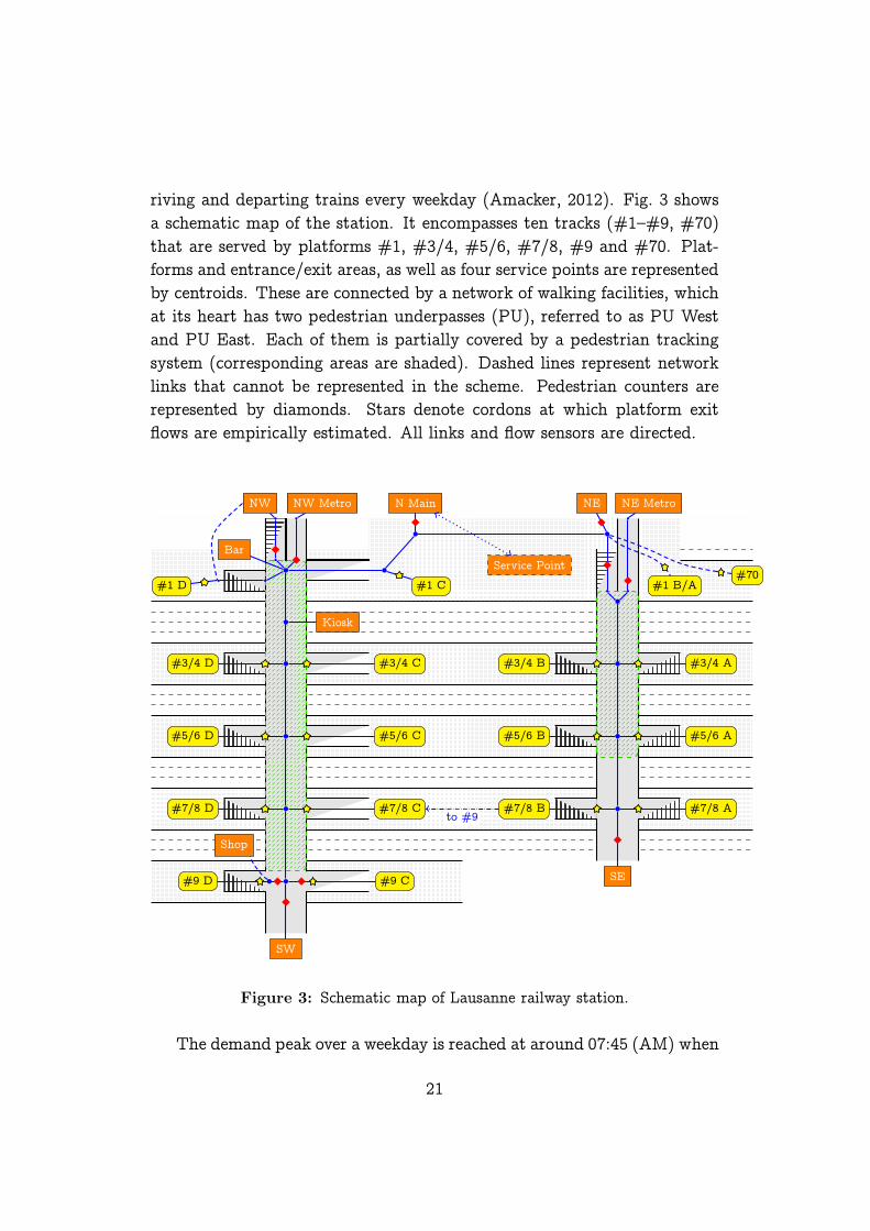
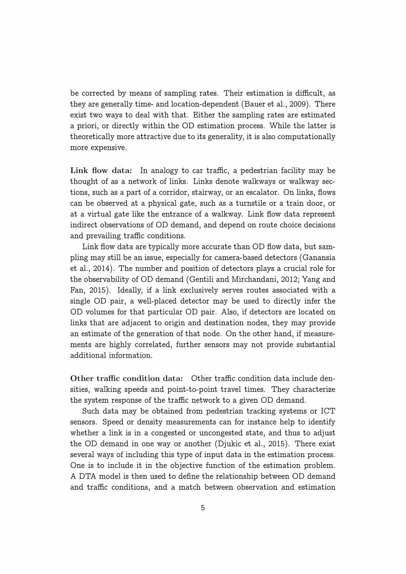
riving and departing trains every weekday (Amacker, 2012). Fig. 3 showsa schematic map of the station. It encompasses ten tracks (#1–#9, #70)that are served by platforms #1, #3/4, #5/6, #7/8, #9 and #70. Plat-forms and entrance/exit areas, as well as four service points are representedby centroids. These are connected by a network of walking facilities, whichat its heart has two pedestrian underpasses (PU), referred to as PU Westand PU East. Each of them is partially covered by a pedestrian trackingsystem (corresponding areas are shaded). Dashed lines represent networklinks that cannot be represented in the scheme. Pedestrian counters arerepresented by diamonds. Stars denote cordons at which platform exitflows are empirically estimated. All links and flow sensors are directed.

#1 D #1 C #1 B/A#70

#3/4 D #3/4 C #3/4 B #3/4 A

#5/6 D #5/6 C #5/6 B #5/6 A

#7/8 D #7/8 C #7/8 B #7/8 A

#9 D #9 C

NW NW Metro N Main NE NE Metro

SW

SE

Shop

Kiosk

Bar

Service Point

to #9

Figure 3: Schematic map of Lausanne railway station.

The demand peak over a weekday is reached at around 07:45 (AM) when

21

several long distance trains arrive and depart in close succession (Gendreand Zulauf, 2010). In the ensuing analysis, we consider the time periodbetween 07:30 and 08:00 with a temporal aggregation of one minute. Datafor a set of 10 ‘reference weekdays’ is available, namely for January 22 and23, February 6, 27 and 28, March 5, as well as April 9, 10, 18 and 30,2013. These dates represent a set of typical weekdays (Tue, Wed, Thu)without major disruptions in the railway system, for which the followingdata sources are available.

OD flow data: Subroute flows are available for the two pedestrian under-passes, in which an elaborate pedestrian tracking system consisting of morethan 60 tracking sensors has been installed. Details of the installation, aswell as of the accuracy of observations, are described by Alahi et al. (2013).OD flow data is used for validation only.

Link flow data: Ten links of the pedestrian walking network, markedby diamonds in Fig. 3, are equipped with sensors that provide directedlink counts with a resolution of one minute. To account for sensor satura-tion, observations are post-processed using a quadratic correction function(Ganansia et al., 2014)

Traffic condition data: Pedestrian trajectories obtained from the afore-mentioned tracking system allow to compute the accumulation in pedes-trian underpasses, which is also used for validation.

Train timetable and ridership data: During the time period of in-terest, a total of 25 trains stop at Lausanne railway station (see Hänseleret al., 2015a, for the train timetable). The actual arrival and departuretime and the assigned track are known for each train and day. An averageestimate of boarding and alighting volumes is available from ticket salesdata, within-train surveys, and infrared-based counts at train doors (SBB-Personenverkehr, 2011). These estimates date back to the year 2010 andare increased by 15% using the official growth rate (Gendre and Zulauf,2010). They are considered as random normal variables with a standarddeviation equal to 19.2% of their mean (Molyneaux et al., 2014).

22

Other data: For the sales points located in PU West (see Fig. 3), anestimate of the number of customer visits is available. There are furtherrestaurants and sales points in the train station building, represented bya generic ‘service point’, for which however no information is available,and which are not considered in the demand analysis. Besides sales data,information on destination split ratios is available (Benmoussa et al., 2011;Anken et al., 2012; Lavadinho et al., 2013).

4.2 Assessment

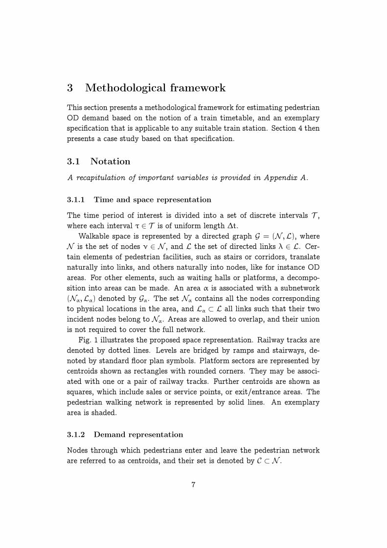
To assess the efficiency of the proposed framework, two estimators are com-pared. A ‘base estimator’, representing a minimum norm solver taking intoaccount link flow data only, and a ‘full estimator’, that additionally con-siders a ‘static’ and a ‘dynamic’ prior (see Fig. 4).

static prior

dynamic prior

travel surveys/sales data

train timetable/ridership data

demand estimatorlink flow data

traffic assignment model

validation

OD flow data

area accumulation data

Figure 4: Scheme of the specification of the demand estimation framework.

The static prior includes cumulative origin and destination flows ob-tained from sales data and platform departure flows, as well as destinationsplit fractions. The dynamic prior represents pre-computed train-inducedarrival flows. OD flow data and traffic condition data are used for vali-dation. In a real context, once the specification is successfully validated,these two data sources would also be integrated in the estimation processto improve the quality of the estimate (dashed arrows in Fig. 4).

23

4.3 Parametrization

The pedestrian walking network of Lausanne railway station disposes of aunique shortest path between every OD pair. During peak periods, regularcommuters constitute the largest user group, which are familiar with thefacilities (Lavadinho, 2012; Ton, 2014). Following Lavadinho (2012), theyalmost exclusively travel along these shortest paths, obviating the need fora route choice model.

To describe the propagation of pedestrians along routes, the walkingspeed distribution proposed by Weidmann (1992),

v ∼ N (1.34 m/s, 0.34 m/s), (29)

is used. It holds for even walking areas; link lengths on inclined areas orstairways need to be adjusted beforehand (Weidmann, 1992). The valid-ity of speed distribution (29) has been empirically verified based on theavailable trajectory recordings, which show no significant signs of demand-supply interaction (Hänseler et al., 2015a).

The schedule-based model is parametrized empirically (Molyneaux et al.,2014). Fig. 5 shows the total exit flow rates observed for platform #3/4, aswell as the corresponding model fit. At low volumes, the flow rate increaseslinearly until a threshold is reached, beyond which the flow rate remainsconstant. The solid curve denotes the predicted flow rate according toEq. (12), and the dashed lines the width of the prediction band in termsof ± one standard deviation.

Two observations may be made. First, the length of a train, measuredin number of passenger cars, ncar, does not have a significant influence onthe flow rate. This is explicitly pointed out since the train length is shownbelow to have a considerable influence on the platform sector split fractionsrsecζ,λ. Second, the flow rates are relatively high, such that the duration of flowis typically below one minute (up to an alighting volume of 333 passengers),and never exceeds 2 min.

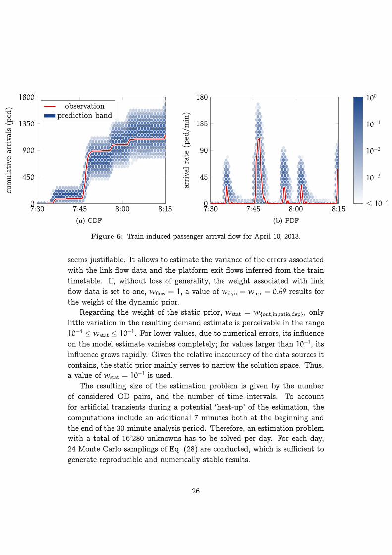
Based on this specification, Fig. 6 shows the predicted exit flow forplatform #5/6 on April 10, 2013, as well as the corresponding observation.The prediction band results from 7500 Monte Carlo samplings of Eq. (6).The alighting volumes eoff

ζ of each train ζ are inferred from the historicalridership data mentioned in Section 4.1. A logarithmic probability densityplot shows the expected cumulative arrivals as well as the arrival rate as a

24

0 200 400 600 8000

200

400

600

alighting volume (ped)

flow

rate

(ped

/min

)

short trains (ncar = 4)long trains (ncar ≥ 7)prediction (Eq. 12)

Figure 5: Total platform exit flow rate f on platform #3/4.

function of time. A good agreement between observation and prediction isfound, although the prediction band is relatively wide. This indicates thatthe variation in alighting volumes across days is high.

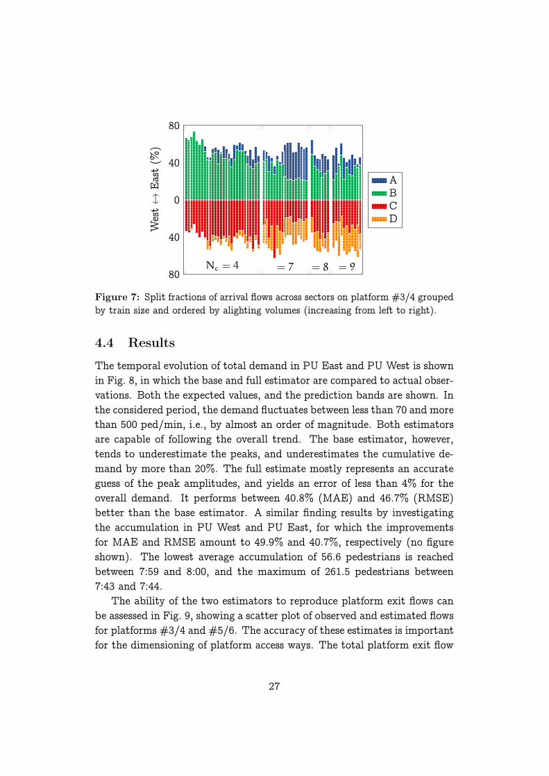
The split fractions rsecζ,λ depend on various factors such as the lengthof a train, its position along a platform, the distribution of passengerswithin a train, as well as their immediate next destination. Fig. 7 showsmeasurements from platform #3/4. The results are grouped by train lengthand ordered by alighting volumes. For short trains with ncar = 4, mostlythe interior platform sectors B and C are used. This is true particularlyif the alighting volume is low. For larger trains with ncar ≥ 7, the lateralsectors absorb a larger share, and the influence of the alighting volume issmaller.

In the framework of this study, two different specifications of the plat-form sector split fractions for short trains (ncar = 4) and long trains(ncar ≥ 7) are considered. For each case, a multivariate normal distri-bution is developed, from which the train- and link-specific platform sectorsplit fractions rsecζ,λ can be drawn (Molyneaux et al., 2014).

The weights of demand indicators in Eq. (28) are determined basedon the premise that pedestrian trajectory recordings represent the truth.Given the accuracy of the trajectory recordings, and their high spatial andtemporal resolution compared to the other data sources, this assumption

25

7:30 7:45 8:00 8:150

450

900

1350

1800

cum

ula

tive

arri

vals

(ped

) observationprediction band

(a) CDF

7:30 7:45 8:00 8:150

45

90

135

180

arri

valra

te(p

ed/m

in)

≤ 10−4

10−3

10−2

10−1

100

(b) PDF

Figure 6: Train-induced passenger arrival flow for April 10, 2013.

seems justifiable. It allows to estimate the variance of the errors associatedwith the link flow data and the platform exit flows inferred from the traintimetable. If, without loss of generality, the weight associated with linkflow data is set to one, wflow = 1, a value of wdyn = warr = 0.69 results forthe weight of the dynamic prior.

Regarding the weight of the static prior, wstat = w{out,in,ratio,dep}, onlylittle variation in the resulting demand estimate is perceivable in the range10−4 ≤ wstat ≤ 10−1. For lower values, due to numerical errors, its influenceon the model estimate vanishes completely; for values larger than 10−1, itsinfluence grows rapidly. Given the relative inaccuracy of the data sources itcontains, the static prior mainly serves to narrow the solution space. Thus,a value of wstat = 10

−1 is used.The resulting size of the estimation problem is given by the number

of considered OD pairs, and the number of time intervals. To accountfor artificial transients during a potential ‘heat-up’ of the estimation, thecomputations include an additional 7 minutes both at the beginning andthe end of the 30-minute analysis period. Therefore, an estimation problemwith a total of 16’280 unknowns has to be solved per day. For each day,24 Monte Carlo samplings of Eq. (28) are conducted, which is sufficient togenerate reproducible and numerically stable results.

26

Nc = 4 = 7 = 8 = 980

40

0

40

80

Wes

t↔

Eas

t(%

)

ABCD

Figure 7: Split fractions of arrival flows across sectors on platform #3/4 groupedby train size and ordered by alighting volumes (increasing from left to right).

4.4 Results

The temporal evolution of total demand in PU East and PU West is shownin Fig. 8, in which the base and full estimator are compared to actual obser-vations. Both the expected values, and the prediction bands are shown. Inthe considered period, the demand fluctuates between less than 70 and morethan 500 ped/min, i.e., by almost an order of magnitude. Both estimatorsare capable of following the overall trend. The base estimator, however,tends to underestimate the peaks, and underestimates the cumulative de-mand by more than 20%. The full estimate mostly represents an accurateguess of the peak amplitudes, and yields an error of less than 4% for theoverall demand. It performs between 40.8% (MAE) and 46.7% (RMSE)better than the base estimator. A similar finding results by investigatingthe accumulation in PU West and PU East, for which the improvementsfor MAE and RMSE amount to 49.9% and 40.7%, respectively (no figureshown). The lowest average accumulation of 56.6 pedestrians is reachedbetween 7:59 and 8:00, and the maximum of 261.5 pedestrians between7:43 and 7:44.

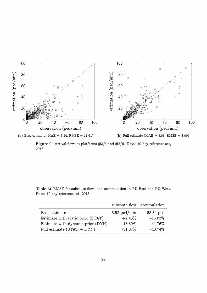
The ability of the two estimators to reproduce platform exit flows canbe assessed in Fig. 9, showing a scatter plot of observed and estimated flowsfor platforms #3/4 and #5/6. The accuracy of these estimates is importantfor the dimensioning of platform access ways. The total platform exit flow

27

07:30 07:40 07:50 08:000

200

400

600

800

dem

and

(ped

/min

)

measuredbase estimate

(a) Base estimate (MAE = 50.74, RMSE = 70.47)

07:30 07:40 07:50 08:000

200

400

600

800

dem

and

(ped

/min

)

measuredfull estimate

(b) Full estimate (MAE = 30.03, RMSE = 37.56)

Figure 8: Total demand in PU East and PU West. Data: 10-day reference set,2013.

is underestimated by the base model by -18.33%, and overestimated by thefull model by 6.98%. The improvement in MAE and RMSE amounts to30.26% and 23.35%, respectively.

Table 3 provides the RMSE for subroute flows and area accumulationsin PU East and PU West for different estimators. Compared to the basemodel, in particular the incorporation of the dynamic prior leads to a sig-nificant improvement. In fact, the consideration of the train timetableincreases the prediction quality more than sales data, information of desti-nation split ratios and cumulative platform departure flows together. Thefull model globally performs best, even though the accumulation estimateis slightly worse than in the case with a dynamic, but no static prior. Sim-ilar findings result if instead of RMSE another statistical measure, such asMAE, is used.

For further details of this case study, see Hänseler et al. (2015a).

28

0 20 40 60 80 1000

20

40

60

80

100

observation (ped/min)

esti

mat

ion

(ped

/min

)

(a) Base estimate (MAE = 7.24, RMSE = 11.61)

0 20 40 60 80 1000

20

40

60

80

100

observation (ped/min)

esti

mat

ion

(ped

/min

)

(b) Full estimate (MAE = 5.05, RMSE = 8.90)

Figure 9: Arrival flows at platforms #3/4 and #5/6. Data: 10-day reference set,2013.

Table 3: RMSE for subroute flows and accumulation in PU East and PU West.Data: 10-day reference set, 2013.

subroute flow accumulation

Base estimate 3.52 ped/min 58.84 pedEstimate with static prior (STAT) +2.43% -15.03%Estimate with dynamic prior (DYN) -15.59% -41.76%Full estimate (STAT + DYN) -31.07% -40.74%

29

5 Conclusions

A framework for the time-dependent estimation of pedestrian origin-destinationdemand within a train station has been presented. Besides direct and indi-rect demand indicators such as flow counts or sales data, the train timetableis explicitly taken into account. This is achieved by establishing an em-pirical relation between the arrival of a train and the subsequent flow ofalighting passengers on platform exit ways. The formulation of the frame-work is such that it can be applied to various types of railway stations andmay be used with different data sources.

A case study of the morning peak period in Lausanne railway station hasbeen presented. The obtained results are in good agreement with pedes-trian tracking data that has been used for validation. A significant perfor-mance gain has been shown to exist when the train timetable is used inthe estimation process. Moreover, spatial and temporal fluctuations, bothintra- and inter-day, have been investigated and are shown to be important,justifying the use of a fully dynamic and probabilistic framework.

We can think of mainly two ways to extend the proposed framework.An obvious way relates to its application to real-time applications, such astraffic monitoring or crowd control. Another way is to focus on the improve-ment of the presented model specification. Clearly, the empirical relationbetween the train timetable and pedestrian movements can be strength-ened, or a demand-dependent network loading model could be integrated.Arguably the most pressing issue, however, is the explicit considerationof correlation among measurements, which could significantly improve thestatistical inference.

Acknowledgement

Financial support by SNSF grant #200021-141099 ‘Pedestrian dynamics:flows and behavior’ and by SBB-CFF-FFS in the framework of ‘PedFlux’,as well as support by Nicolas Anken, Quentin Mazars-Simon, Bonnie Qian,Eduard Rojas and Amanda Stathopoulos in implementing the case studyof Lausanne railway station is gratefully acknowledged.

30

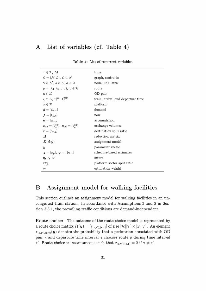
A List of variables (cf. Table 4)

Table 4: List of recurrent variables.

τ ∈ T , ∆t time

G = (N ,L), C ⊂ N graph, centroids

ν ∈ N , λ ∈ L, α ∈ A node, link, area

ρ = (λ1, λ2, . . . ), ρ ∈ R route

κ ∈ K OD pair

ζ ∈ Z, tarrζ , tdepζ train, arrival and departure time

π ∈ P platform

d = [dκ,τ] demand

f = [fλ,τ] flow

a = [aα,τ] accumulation

eon = [eonζ ], eoff = [eoffζ ] exchange volumes

r = [rν,τ] destination split ratio

∆ reduction matrix

Σ(d;y) assignment model

y parameter vector

χ = [χp], ϕ = [φλ,τ] schedule-based estimates

η, ε, ω errors

rsecζ,λ platform sector split ratio

w estimation weight

B Assignment model for walking facilities

This section outlines an assignment model for walking facilities in an un-congested train station. In accordance with Assumptions 2 and 3 in Sec-tion 3.3.1, the prevailing traffic conditions are demand-independent.

Route choice: The outcome of the route choice model is represented bya route choice matrix R(y) = [r(ρ,τ′),(κ,τ)] of size |R||T |×|Z||T |. An elementr(ρ,τ′),(κ,τ)(y) denotes the probability that a pedestrian associated with ODpair κ and departure time interval τ chooses route ρ during time intervalτ′. Route choice is instantaneous such that r(ρ,τ′),(κ,τ) = 0 if τ 6= τ′.

31

The time to traverse link λ during time interval τ is denoted by ∆ttravλ,τ (y).The travel time on route ρ during time interval τ is given by

Uρ,τ(y) = Vρ,τ + ψ, (30)

where ψ ∼ EV(0, ϑ) with ϑ a calibration parameter contained in y, andwhere the sum of link travel times is given by

Vρ,τ(y) =∑

λ∈ρ

∆ttravλ,τ . (31)

For OD pair κ, the likelihood that a user chooses route ρ ∈ Rκ is thengiven by

r(ρ,τ),(κ,τ)(y) =exp(−ϑVρ,τ)∑

ρ′∈Rκexp(−ϑVρ′ ,τ)

. (32)

Network loading: The network loading model defines mappings fromroute flows to link flows and area accumulations. Table 5 defines the cor-responding assignment matrices.

Table 5: List of considered network loading maps.

B = [b(λ,τ′),(ρ,τ)] The link flow assignment matrix B(y) is of size |Λ||T | × |R||T |.The entry b(λ,τ′),(ρ,τ)(y) represents the probability that a pedes-trian associated with route ρ and departure time interval τreaches link λ during time interval τ′.

C = [c(α,τ′),(ρ,τ)] The area accumulation assignment matrix C(y) is of size |A||T |×

|R||T |. The entry c(α,τ′),(ρ,τ)(y) denotes the expected contribu-tion of a pedestrian associated with route ρ and departure timeinterval τ to the accumulation of area α during time interval τ′.

Based on these definitions, we may write

Σf(d;y) = B(y)R(y)d, (33)

andΣa(d;y) = C(y)R(y)d, (34)

respectively.Let the distance along a route ρ up to the beginning of link λ be de-

noted by ℓλρ. Furthermore, let the departure times of pedestrians within a

32

time interval be distributed uniformly, i.e., the distribution of continuousdeparture time t for any route during a time interval τ is given by

hτ(t) =

{1∆t

if t ∈ τ,

0 otherwise.(35)

Assuming that each pedestrian is walking at a constant speed, the proba-bility for a person on route ρ that departs during time interval τ to arriveon link λ during time interval τ′ is given by

b(λ,τ′),(ρ,τ) = Pr(t ∈ τ, t′ ∈ τ′|ρ, λ)

= Pr

(

t ∈ τ, v ∈

[

ℓλρ

t+τ′ − t,ℓλρ

t−τ′ − t

])

, (36)

where t−τ and t+τ represent the bounds of time interval τ, and where t and t′

represent the continuous departure and arrival time, respectively. For themost common case that ℓλρ > 0 and τ′ > τ, we obtain

b(λ,τ′),(ρ,τ) =

∫ t+τ

t=t−τ

∫ ℓλρ/(t−τ′−t)

v=ℓλρ/(t+

τ′−t)

fv(v)gτ(t) dv dt

=1

∆t

∫ t+τ

t=t−τ

Fv

(

ℓλρ

t−τ′ − t

)

− Fv

(

ℓλρ

t+τ′ − t

)

dt. (37)

Similarly, if ℓλρ > 0 and τ = τ′, we obtain

b(λ,τ),(ρ,τ) = 1− Pr (t ∈ τ, t′ 6∈ τ|ρ, λ)

= 1− Pr

(

t ∈ τ, v ∈

[

0,ℓλρ

t+τ − t

])

= 1−1

∆t

∫ t+τ

t=t−τ

Fv

(

ℓλρ

t+τ − t

)

− Fv(0) dt. (38)

Thus, the probability that a user associated with route ρ and departuretime interval τ reaches link λ during time interval τ′ is given by

b(λ,τ′),(ρ,τ) =

0 if ℓλρ = 0, τ < τ′,

1 if ℓλρ = 0, τ = τ′,

Eq. (37) if ℓλρ > 0, τ < τ′,

Eq. (38) if ℓλρ > 0, τ = τ′.

(39)

33

Remark: The probability that a pedestrian associated with route ρ anddeparture time interval τ reaches subroute during time interval τ′ can beexpressed as

g(,τ′),(ρ,τ) =

{b(λo

,τ′),(ρ,τ) if ∈ Rsub

ρ ,

0 otherwise,(40)

where Rsubρ denotes the set of subroutes contained in route ρ, and λo

the

first link of subroute .The assignment fraction for area accumulations can be derived accord-

ingly. Let us consider an area α, and let us assume that each route entersand leaves area α at most once. Let v be the constant, individual speedof a person traveling along route ρ, ℓρ,αin the distance along the route ρ tothe entrance of area α and ℓρ,αout the corresponding distance to its exit. Con-sequently, tin = ℓρ,αin /v is the time after departure at which a person withspeed v enters area α and tout = ℓ

ρ,αout/v the corresponding time at which it

is exited. If a route ρ does not cross area α, then ℓρ,αin = ∞. If we considera time interval [t−, t+] after departure, the expected sojourn time for thisperson with constant speed v inside the area α within the interval is givenby

σ(v, ℓρ,αin , ℓρ,αout, t

−, t+) =

t+ − ℓρ,αin /v if t− ≤ ℓρ,αin /v ≤ t+ ≤ ℓρ,αout/v,

ℓρ,αout/v− t− if ℓρ,αin /v ≤ t

− ≤ ℓρ,αout/v ≤ t+,

t+ − t− if ℓρ,αin /v ≤ t− ≤ t+ ≤ ℓρ,αout/v,

(ℓρ,αout − ℓρ,αin )/v if t− ≤ ℓρ,αin /v ≤ ℓ

ρ,αout/v ≤ t

+,

0 otherwise.

(41)

In Eq. (41), the first line corresponds to the case where a person reaches thearea within the time interval, but does not exit it. The second line is theinverse case. The third line represents the case where a person stays withinthe area during the full time period. Finally, the fourth line represents thecase where a pedestrian enters and leaves the area during the period ofinterest, and the fifth case the situation where a pedestrian is not presentin area α during the time interval at all.

Using Eq. (41), the expected contribution of a pedestrian traveling alongroute ρ with departure time interval τ to the accumulation of area α during

34

time interval τ′ is given by

c(α,τ′),(ρ,τ) =

∫ t+τ

t=t−τ

∫∞

v=0

σ(v, ℓρ,αin , ℓρ,αout, t

−τ′ − t, t

+τ′ − t)

∆tfv(v)hτ(t) dv dt

=1

∆t2

∫∞

v=0

fv(v)

∫ t+τ

t=t−τ

σ(v, ℓρ,αin , ℓρ,αout, t

−τ′ − t, t

+τ′ − t) dt dv. (42)

For an efficient implementation, we note that the assignment fractions (39)and (42) are time-invariant, i.e., for ∆τ = τ′ − τ it holds that

b(λ,τ′),(ρ,τ) = b(λ,∆τ),(ρ,0) and c(α,τ′),(ρ,τ) = c(α,∆τ),(ρ,0). (43)

To further reduce the cost involved in computing Eq. (39) and Eq. (42), amaximum travel time TTmax is defined. If ∆τ ≥ TTmax, it is assumed thatb(λ,∆τ),(ρ,0) = 0 ∀ λ, ρ and c(α,∆τ),(ρ,0) = 0 ∀α, ρ. The threshold TTmax is chosensuch that the error incurred by this numerical approximation is negligible.

References

Alahi, A., Bierlaire, M., Vandergheynst, P., 2014. Robust real-time pedes-trians detection in urban environments with low-resolution cameras.Transportation Research Part C: Emerging Technologies 39, 113–128.

Alahi, A., Ramanathan, V., Fei-Fei, L., 2013. Socially-aware large-scalecrowd forecasting. In: Proceedings of the IEEE Conference on ComputerVision and Pattern Recognition. pp. 2203–2210.

Amacker, K., 2012. SBB Facts and Figures. Annual report, Swiss FederalRailways (SBB-CFF-FFS), Bern, Switzerland.

Anken, N., Hänseler, F. S., Bierlaire, M., 2012. Flux piétonniers dans lagare de Lausanne: Vers l’estimation d’une matrice OD à l’aide des ex-trapolations voyageurs des CFF. Internal report (unpublished), EcolePolytechnique Fédérale de Lausanne.

Antonini, G., Bierlaire, M., Weber, M., 2006. Discrete choice models ofpedestrian walking behavior. Transportation Research Part B: Method-ological 40 (8), 667–687.

35

Ashok, K., Ben-Akiva, M. E., 2000. Alternative approaches for real-timeestimation and prediction of time-dependent origin–destination flows.Transportation Science 34 (1), 21–36.

Bauer, D., Brändle, N., Seer, S., Ray, M., Kitazawa, K., 2009. Measurementof pedestrian movements: A comparative study on various existing sys-tems. Pedestrian Behavior: Models, Data Collection and Applications.

Ben-Akiva, M. E., Bierlaire, M., 2003. Discrete choice models with appli-cations to departure time and route choice. Handbook of TransportationScience 32.

Benmoussa, M., Ducommun, F., Khalfi, A., Kharouf, M., Koymans, A.,Nguyen, M., Raies, A., Vidaud, M., Birchler, C., 2011. Analyse desflux piétonniers en gare de Lausanne. Tech. rep., Ecole PolytechniqueFédérale de Lausanne.

Bierlaire, M., Crittin, F., 2004. An efficient algorithm for real-time estima-tion and prediction of dynamic OD tables. Operations Research 52 (1),116–127.

Bierlaire, M., Crittin, F., 2006. Solving noisy, large-scale fixed-point prob-lems and systems of nonlinear equations. Transportation Science 40 (1),44–63.

Bierlaire, M., Robin, T., 2009. Pedestrians choices. Pedestrian Behavior.Models, Data Collection and Applications, 1–26.

Bierlaire, M., Toint, P. L., 1995. Meuse: An origin-destination matrix esti-mator that exploits structure. Transportation Research Part B: Method-ological 29 (1), 47–60.

Bierlaire, M., Toint, P. L., Tuyttens, D., 1991. On iterative algorithms forlinear least squares problems with bound constraints. Linear Algebra andits Applications 143, 111–143.

Blue, V. J., Adler, J. L., 2001. Cellular automata microsimulation for mod-eling bi-directional pedestrian walkways. Transportation Research PartB: Methodological 35 (3), 293–312.

36

Buchmüller, S., Weidmann, U., 2008. Handbuch zur Anordnung und Di-mensionierung von Fussgängeranlagen in Bahnhöfen. IVT Projekt Nr. C-06-07. Institute for Transport Planning and Systems, ETH Zürich,Switzerland.

Cascetta, E., 1984. Estimation of trip matrices from traffic counts and sur-vey data: A generalized least squares estimator. Transportation ResearchPart B: Methodological 18 (4), 289–299.

Cascetta, E., Improta, A. A., 2002. Estimation of travel demand usingtraffic counts and other data sources. Applied Optimization 63, 71–91.

Cascetta, E., Inaudi, D., Marquis, G., 1993. Dynamic estimators of origin-destination matrices using traffic counts. Transportation Science 27 (4),363–373.

Cascetta, E., Nguyen, S., 1988. A unified framework for estimating or up-dating origin/destination matrices from traffic counts. TransportationResearch Part B: Methodological 22 (6), 437–455.

Cascetta, E., Nuzzolo, A., Russo, F., Vitetta, A., 1996. A modified logitroute choice model overcoming path overlapping problems: Specificationand some calibration results for interurban networks. In: Proceedings ofthe 13th International Symposium on Transportation and Traffic Theory.Pergamon, pp. 697–711.

Cascetta, E., Papola, A., Marzano, V., Simonelli, F., Vitiello, I., 2013.Quasi-dynamic estimation of o–d flows from traffic counts: Formulation,statistical validation and performance analysis on real data. Transporta-tion Research Part B: Methodological 55, 171–187.

Cascetta, E., Postorino, M. N., 2001. Fixed point approaches to the es-timation of O/D matrices using traffic counts on congested networks.Transportation Science 35 (2), 134–147.

Casey, H. J., 1955. Applications to traffic engineering of the law of retailgravitation. Traffic Quarterly 9 (1), 23–35.

Cheung, C. Y., Lam, W. H. K., 1998. Pedestrian route choices betweenescalator and stairway in MTR stations. Journal of Transportation En-gineering 124 (3), 277–285.

37

Cule, B., Goethals, B., Tassenoy, S., Verboven, S., 2011. Mining train de-lays. In: Advances in Intelligent Data Analysis X. Springer, pp. 113–124.

Daamen, W., 2004. Modelling passenger flows in public transport facilities.Ph.D. thesis, Delft University of Technology.

Daamen, W., Bovy, P. H. L., Hoogendoorn, S. P., 2005. Influence of changesin level on passenger route choice in railway stations. Transportation Re-search Record: Journal of the Transportation Research Board 1930 (1),12–20.

Daly, P. N., McGrath, F., Annesley, T. J., 1991. Pedestrian speed/flowrelationships for underground stations. Traffic Engineering & Control32 (2), 75–78.

Danalet, A., Farooq, B., Bierlaire, M., 2014. A Bayesian approach to detectpedestrian destination-sequences from WiFi signatures. TransportationResearch Part C: Emerging Technologies 44, 146–170.

Davidich, M., Geiss, F., Mayer, H. G., Pfaffinger, A., Royer, C., 2013. Wait-ing zones for realistic modelling of pedestrian dynamics: A case studyusing two major German railway stations as examples. TransportationResearch Part C: Emerging Technologies 37, 210–222.

Dial, R. B., 1971. A probabilistic multipath traffic assignment model whichobviates path enumeration. Transportation Research 5 (2), 83–111.

Djukic, T., Barceló, J., Bullejos, M., Montero, L., Cipriani, E., van Lint, H.,Hoogendoorn, S. P., 2015. Advanced traffic data for dynamic od demandestimation: The state of the art and benchmark study. TransportationResearch Record: Journal of the Transportation Research Board.

Djukic, T., Flötteröd, G., van Lint, H., Hoogendoorn, S. P., 2012. Efficientreal time od matrix estimation based on principal component analysis.In: Intelligent Transportation Systems (ITSC), 2012 15th InternationalIEEE Conference on. IEEE, pp. 115–121.

Edie, L. C., 1963. Discussion of traffic stream measurements and definitions.Proceedings of the Second International Symposium on the Theory ofTraffic Flow, 139–154.

38

Fisk, C. S., 1988. On combining maximum entropy trip matrix estimationwith user optimal assignment. Transportation Research Part B: Method-ological 22 (1), 69–73.

Florian, M., Chen, Y., 1995. A Coordinate Descent Method for the Bi-level O–D Matrix Adjustment Problem. International Transactions inOperational Research 2 (2), 165–179.

Frejinger, E., Bierlaire, M., 2007. Capturing correlation with subnetworksin route choice models. Transportation Research Part B: Methodological41 (3), 363–378.

Ganansia, F., Carincotte, C., Descamps, A., Chaudy, C., 2014. A promisingapproach to people flow assessment in railway stations using standardCCTV networks. In: Transport Research Arena, Paris.

Gendre, G., Zulauf, C., 2010. Gare de Lausanne: Analyse des flux piéton-niers. Internal report (I-PM-LS; unpublished), Swiss Federal Railways(SBB-CFF-FFS), Lausanne, Switzerland.

Gentili, M., Mirchandani, P. B., 2012. Locating sensors on traffic networks:Models, challenges and research opportunities. Transportation ResearchPart C: Emerging Technologies 24, 227–255.

Goverde, R. M. P., 2007. Railway timetable stability analysis using max-plus system theory. Transportation Research Part B: Methodological41 (2), 179–201.

Hänseler, F. S., Bierlaire, M., Farooq, B., Mühlematter, T., 2014. A macro-scopic loading model for time-varying pedestrian flows in public walkingareas. Transportation Research Part B: Methodological 69, 60–80.

Hänseler, F. S., Bierlaire, M., Molyneaux, N. A., Scarinci, R., Thémans,M., 2015a. Modeling pedestrian flows in train stations: The exampleof Lausanne railway station. Proceedings of the 15th Swiss TransportResearch Conference.

Hänseler, F. S., Molyneaux, N. A., Bierlaire, M., 2015b. Python implemen-tation of pedestrian OD demand estimator for train stations.URL https://github.com/flurinus/DemEstMeth

39

Hazelton, M. L., 2000. Estimation of origin–destination matrices fromlink flows on uncongested networks. Transportation Research Part B:Methodological 34 (7), 549–566.

Hazelton, M. L., 2003. Some comments on origin–destination matrix esti-mation. Transportation Research Part A: Policy and Practice 37 (10),811–822.

Helbing, D., Molnár, P., 1995. Social force model for pedestrian dynamics.Physical Review E 51 (5), 4282–4286.

Higgins, A., Kozan, E., 1998. Modeling train delays in urban networks.Transportation Science 32 (4), 346–357.

Highway Capacity Manual, 2000. Transportation Research Board. Wash-ington, DC.

Hoogendoorn, S. P., Bovy, P. H. L., 2004. Pedestrian route-choice andactivity scheduling theory and models. Transportation Research Part B:Methodological 38 (2), 169–190.

Hoogendoorn, S. P., Daamen, W., 2004. Design assessment of Lisbon trans-fer stations using microscopic pedestrian simulation. In: Computers inrailways IX (Congress Proceedings of CompRail 2004). pp. 135–147.

Hughes, R. L., 2002. A continuum theory for the flow of pedestrians. Trans-portation Research Part B: Methodological 36 (6), 507–535.

Kaakai, F., Hayat, S., El Moudni, A., 2007. A hybrid Petri nets-basedsimulation model for evaluating the design of railway transit stations.Simulation Modelling Practice and Theory 15 (8), 935–969.

Lam, W. H. K., Wu, Z. X., Chan, K. S., 2003. Estimation of transit origin–destination matrices from passenger counts using a frequency-based ap-proach. Journal of Mathematical Modelling and Algorithms 2 (4), 329–348.

Lavadinho, S., 2012. Compréhension fine des stratégies piétonnières engare de Lausanne. Internal report (unpublished), Swiss Federal Railways(SBB-CFF-FFS), Lausanne, Switzerland.

40

Lavadinho, S., Alahi, A., Bagnato, L., 2013. Analysis of Pedestrian Flows:Underground pedestrian walkways of Lausanne train station. Internalreport (unpublished), VisioSafe SA, Switzerland.

Lawson, C. L., Hanson, R. J., 1974. Solving least squares problems. Vol.161. Society for Industrial and Applied Mathematics.

Lee, J. Y. S., Lam, W. H. K., Wong, S. C., 2001. Pedestrian simulationmodel for Hong Kong underground stations. In: Intelligent Transporta-tion Systems. IEEE, pp. 554–558.

Løvås, G. G., 1994. Modeling and simulation of pedestrian traffic flow.Transportation Research Part B: Methodological 28 (6), 429–443.

Marzano, V., Papola, A., Simonelli, F., 2009. Limits and perspectives ofeffective o–d matrix correction using traffic counts. Transportation Re-search Part C: Emerging Technologies 17 (2), 120–132.

Molyneaux, N. A., Hänseler, F. S., Bierlaire, M., 2014. Modeling of train-induced pedestrian flows in railway stations. Proceedings of the 14thSwiss Transport Research Conference.

Montero, L., Codina, E., Barceló, J., 2015. Dynamic od transit matrixestimation: formulation and model-building environment. In: Progressin Systems Engineering. Springer, pp. 347–353.

Mustafa, M., Ashaari, Y., 2015. Assessing pedestrian behavioral patternat rail transit terminal: State of the art. In: Proceedings of the Inter-national Civil and Infrastructure Engineering Conference. Springer, pp.1245–1254.

Nguyen, S., Morello, E., Pallottino, S., 1988. Discrete time dynamic estima-tion model for passenger origin/destination matrices on transit networks.Transportation Research Part B: Methodological 22 (4), 251–260.

Pettersson, P., 2011. Passenger waiting strategies on railway platforms:Effects of information and platform facilities. Master’s thesis, KTH.

Rindsfüser, G., Klügl, F., 2007. Agent-based pedestrian simulation: A casestudy of Bern Railway Station. The Planning Review 170, 9–18.

41

SBB-Personenverkehr, 2011. SBB Clearing Extrapolation Voyageurs HOP.Internal report (unpublished), Swiss Federal Railways (SBB-CFF-FFS),Bern, Switzerland.

Starmans, M., Verhoeff, L., van den Heuvel, J. P. A., 2014. Passengertransfer chain analysis for reallocation of heritage space at AmsterdamCentral station. Transportation Research Procedia 2, 651–659.

Ton, D., 2014. NAVISTATION: A study into the route and activity loca-tion choice behaviour of departing pedestrians in train stations. Master’sthesis, Delft University of Technology.

Turner, S., Middleton, D., Longmire, R., Brewer, M., Eurek, R., 2007.Testing and evaluation of pedestrian sensors. Monograph, TransportationResearch Board.

U.S. Department of Transportation, 2013. Traffic monitoring guide. Tech.rep., Federal Highway Administration.

van den Heuvel, J. P. A., Hoogenraad, J. H., 2014. Monitoring the perfor-mance of the pedestrian transfer function of train stations using auto-matic fare collection data. Transportation Research Procedia 2, 642–650.

van Hagen, M., 2011. Waiting experience at train stations. Ph.D. thesis,Universiteit Twente.

van Zuylen, H. J., Willumsen, L. G., 1980. The most likely trip matrixestimated from traffic counts. Transportation Research Part B: Method-ological 14 (3), 281–293.

Weidmann, U., 1992. Transporttechnik der Fussgänger. Schriftenreihe desIVT Nr. 90. Institute for Transport Planning and Systems, ETH Zürich,Switzerland.

Willumsen, L. G., 1981. An entropy maximising model for estimating tripmatrices from traffic counts. Ph.D. thesis, University of Leeds.

Wilson, A. G., 1970. Entropy in urban and regional modelling. Pion Press.

Wong, S. C., Tong, C., 1998. Estimation of time-dependent origin–destination matrices for transit networks. Transportation Research PartB: Methodological 32 (1), 35–48.

42

Wong, S. C., Tong, C. O., Wong, K. I., Lam, W. H. K., Lo, H. K., Yang,H., Lo, H. P., 2005. Estimation of multiclass origin-destination matricesfrom traffic counts. Journal of Urban Planning and Development 131 (1),19–29.

Xu, X. Y., Liu, J., Li, H. Y., Hu, J. Q., 2014. Analysis of subway stationcapacity with the use of queueing theory. Transportation Research PartC: Emerging Technologies 38, 28–43.

Yang, H., 1995. Heuristic algorithms for the bilevel origin-destination ma-trix estimation problem. Transportation Research Part B: Methodologi-cal 29 (4), 231–242.

Yang, Y., Fan, Y., 2015. Data dependent input control for origin–destination demand estimation using observability analysis. Transporta-tion Research Part B: Methodological 78, 385–403.

Yuan, J., Hansen, I. A., 2007. Optimizing capacity utilization of stationsby estimating knock-on train delays. Transportation Research Part B:Methodological 41 (2), 202–217.

Zhou, X., Mahmassani, H. S., 2007. A structural state space model forreal-time traffic origin–destination demand estimation and predictionin a day-to-day learning framework. Transportation Research Part B:Methodological 41 (8), 823–840.

43