


Languages
Pages
Legal


Copyright © 2010, 2007, 2004 Pearson Education, Inc. 13.1 - 1
Lecture Slides
Elementary Statistics Eleventh Edition
and the Triola Statistics Series
by Mario F. Triola

Copyright © 2010, 2007, 2004 Pearson Education, Inc. 13.1 - 2
Chapter 13Nonparametric Statistics
13-1 Review and Preview
13-2 Sign Test
13-3 Wilcoxon Signed-Ranks Test for Matched Pairs
13-4 Wilcoxon Rank-Sum Test for Two Independent Samples
13-5 Kruskal-Wallis Test
13-6 Rank Correction
13-7 Runs Test for Randomness

Copyright © 2010, 2007, 2004 Pearson Education, Inc. 13.1 - 3
Section 13- 4 Wilcoxon Rank-Sum Test
for Two Independent Samples

Copyright © 2010, 2007, 2004 Pearson Education, Inc. 13.1 - 4
Key Concept
The Wilcoxon rank-sum test uses ranks of values from two independent samples to test the null hypothesis that the two populations have equal medians.

Copyright © 2010, 2007, 2004 Pearson Education, Inc. 13.1 - 5
Key Concept
The basic idea underlying the Wilcoxon rank-sum test is this: If two samples are drawn from identical populations and the individual values are all ranked as one combined collection of values, then the high and low ranks should fall evenly between the two samples. If the low ranks are found predominantly in one sample and the high ranks are found predominantly in the other sample, we suspect that the two populations have different medians.

Copyright © 2010, 2007, 2004 Pearson Education, Inc. 13.1 - 6
Basic Concept
If two samples are drawn from identical populations and the individual values are all ranked as one combined collection of values, then the high and low ranks should fall evenly between the two samples.

Copyright © 2010, 2007, 2004 Pearson Education, Inc. 13.1 - 7
Caution
Don’t confuse the Wilcoxon rank-sum test for two independent samples with the Wilcoxon signed-ranks test for matched pairs. Use Internal Revenue Service as the mnemonic for IRS to remind us of “Independent: Rank Sum.”

Copyright © 2010, 2007, 2004 Pearson Education, Inc. 13.1 - 8
Definition
The Wilcoxon rank-sum test is a nonparametric test that uses ranks of sample data from two independent populations. It is used to test the null hypothesis that the two independent samples come from populations with equal medians.
: The two samples come from populations with equal medians. : The two samples come from populations with different medians.
0H
1H
Copyright © 2010, 2007, 2004 Pearson Education, Inc. 13.1 - 9
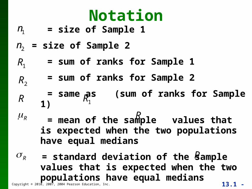
= size of Sample 1
= size of Sample 2
= sum of ranks for Sample 1
= sum of ranks for Sample 2
= same as (sum of ranks for Sample 1)
= mean of the sample values that is expected when the two populations have equal medians
= standard deviation of the sample values that is expected when the two populations have equal medians
Notation1n
1R
2n
2R
R 1R
RR
R R
Copyright © 2010, 2007, 2004 Pearson Education, Inc. 13.1 - 10
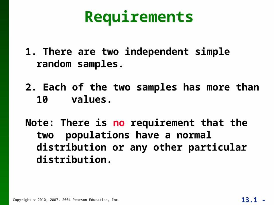
Requirements
1. There are two independent simple random samples.
2. Each of the two samples has more than 10 values.
Note: There is no requirement that the two populations have a normal distribution or any other particular distribution.
Copyright © 2010, 2007, 2004 Pearson Education, Inc. 13.1 - 11
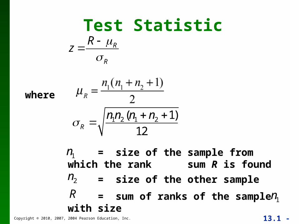
Test Statistic
where
= size of the sample from which the rank sum R is found
= size of the other sample
= sum of ranks of the sample with size
R
R
Rz
1 2 1 2( 1)
12R
n n n n
1n
2n
R1n

Copyright © 2010, 2007, 2004 Pearson Education, Inc. 13.1 - 12
Critical values can be found in Table A-2 (because the test statistic is based on the normal distribution).
P-Values can be found using the z test statistic and Table A-2.
Critical and P-Values for the Wilcoxon Rank-Sum Test
Copyright © 2010, 2007, 2004 Pearson Education, Inc. 13.1 - 13
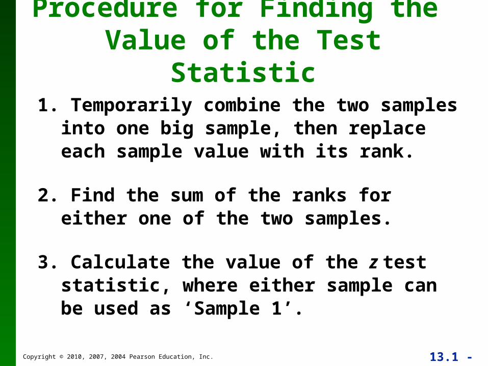
Procedure for Finding the Value of the Test Statistic
1. Temporarily combine the two samples into one big sample, then replace each sample value with its rank.
2. Find the sum of the ranks for either one of the two samples.
3. Calculate the value of the z test statistic, where either sample can be used as ‘Sample 1’.

Copyright © 2010, 2007, 2004 Pearson Education, Inc. 13.1 - 14
Table 13-5 lists the braking distances (in ft) of samples of 4-cylinder cars and 6-cylinder cars Use a 0.05 significance level to test the claim that 4-cylinder cars and 6-cylinder cars have the same median braking distance. The numbers in parentheses are their ranks beginning with a rank of 1 assigned to the lowest value of 122. and at the bottom denote the sum of ranks.
Example:
1R 2R
Copyright © 2010, 2007, 2004 Pearson Education, Inc. 13.1 - 15
Example:
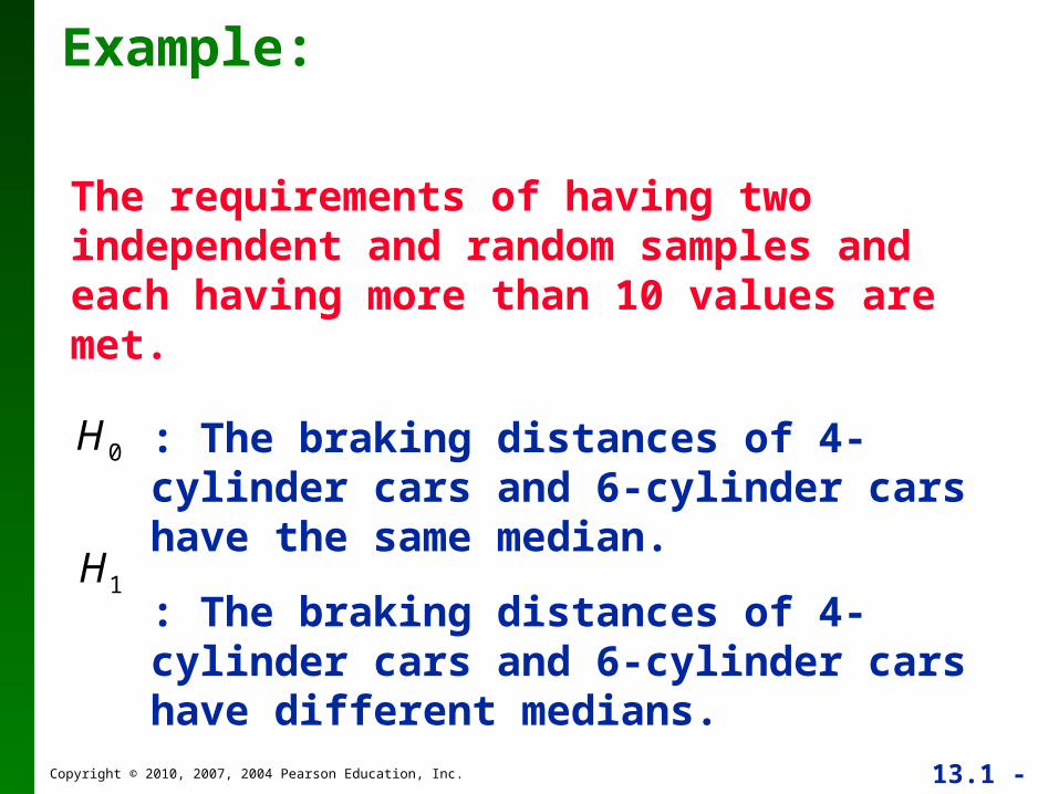
The requirements of having two independent and random samples and each having more than 10 values are met.
: The braking distances of 4-cylinder cars and 6-cylinder cars have the same median.
: The braking distances of 4-cylinder cars and 6-cylinder cars have different medians.
0H
1H

Copyright © 2010, 2007, 2004 Pearson Education, Inc. 13.1 - 16
Example:
Procedure
1. Rank all 25 braking distances of cars combined. This is done in Table 13-5.
2. Find the sum of the ranks of either one of the samples. For 4-cylinder cars it is
12.5 23 ... 11 180.5R
Copyright © 2010, 2007, 2004 Pearson Education, Inc. 13.1 - 17
Example:
Procedure (cont.)
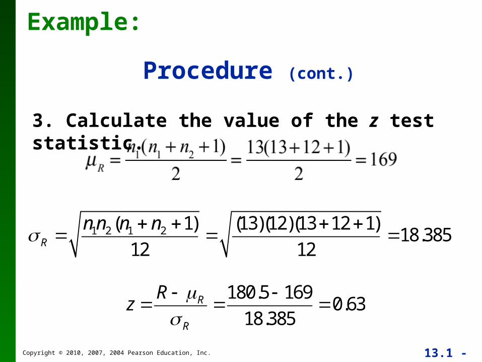
3. Calculate the value of the z test statistic.
1 2 1 2( 1) (13)(12)(13 12 1)18.385
12 12R
n n n n
180.5 1690.63
18.385R
R
Rz

Copyright © 2010, 2007, 2004 Pearson Education, Inc. 13.1 - 18
Example:
The test is two-tailed because a large positive value of z would indicate that the higher ranks are found disproportionately in Sample 1, and a large negative value of z would indicate that disproportionately more lower ranks are found in Sample 1.
In either case, we would have strong evidence against the claim that the two samples come from populations with equal medians.
Copyright © 2010, 2007, 2004 Pearson Education, Inc. 13.1 - 19
Example:
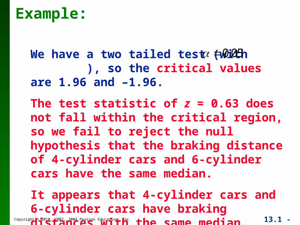
We have a two tailed test (with ), so the critical values are 1.96 and –1.96.
The test statistic of z = 0.63 does not fall within the critical region, so we fail to reject the null hypothesis that the braking distance of 4-cylinder cars and 6-cylinder cars have the same median.
It appears that 4-cylinder cars and 6-cylinder cars have braking distances with the same median.
0.05
Copyright © 2010, 2007, 2004 Pearson Education, Inc. 13.1 - 20
Recap
In this section we have discussed:
The Wilcoxon Rank-Sum Test for Two Independent Samples.
It is used to test the null hypothesis that the two independent samples come from populations with equal medians.
Top Related