


Languages
Pages
Legal


Copyright ©2012 Pearson Education, Inc. publishing as Prentice Hall Chap 5-1Chap 5-1
Chapter 5
Discrete Probability Distributions
Basic Business Statistics12th Edition

Chap 5-2Copyright ©2012 Pearson Education, Inc. publishing as Prentice Hall Chap 5-2
Learning Objectives
In this chapter, you learn: The properties of a probability distribution To compute the expected value and variance of a
probability distribution To calculate the covariance and understand its use
in finance To compute probabilities from binomial,
hypergeometric, and Poisson distributions How to use the binomial, hypergeometric, and
Poisson distributions to solve business problems

Chap 5-3Copyright ©2012 Pearson Education, Inc. publishing as Prentice Hall Chap 5-3
DefinitionsRandom Variables
A random variable represents a possible numerical value from an uncertain event.
Discrete random variables produce outcomes that come from a counting process (e.g. number of classes you are taking).
Continuous random variables produce outcomes that come from a measurement (e.g. your annual salary, or your weight).

Chap 5-4Copyright ©2012 Pearson Education, Inc. publishing as Prentice Hall Chap 5-4
DefinitionsRandom Variables
Random Variables
Discrete Random Variable
ContinuousRandom Variable
Ch. 5 Ch. 6
DefinitionsRandom Variables
Random Variables
Discrete Random Variable
ContinuousRandom Variable
Ch. 5 Ch. 6
DefinitionsRandom Variables
Random Variables
Discrete Random Variable
ContinuousRandom Variable
Ch. 5 Ch. 6

Chap 5-5Copyright ©2012 Pearson Education, Inc. publishing as Prentice Hall Chap 5-5
Discrete Random Variables
Can only assume a countable number of values
Examples:
Roll a die twiceLet X be the number of times 4 occurs (then X could be 0, 1, or 2 times)
Toss a coin 5 times. Let X be the number of heads
(then X = 0, 1, 2, 3, 4, or 5)

Chap 5-6Copyright ©2012 Pearson Education, Inc. publishing as Prentice Hall Chap 5-6
Probability Distribution For A Discrete Random Variable
A probability distribution for a discrete random variable is a mutually exclusive listing of all possible numerical outcomes for that variable and a probability of occurrence associated with each outcome.
Number of Classes Taken Probability
2 0.20
3 0.40
4 0.24
5 0.16
Chap 5-7Copyright ©2012 Pearson Education, Inc. publishing as Prentice Hall Chap 5-7
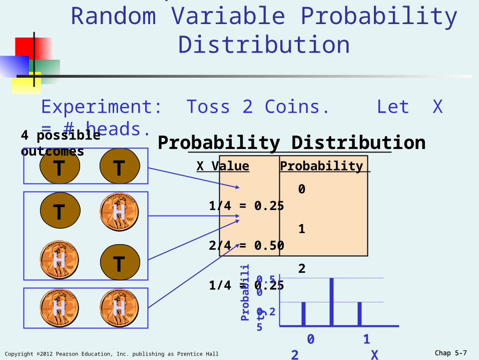
Experiment: Toss 2 Coins. Let X = # heads.
T
T
Example of a Discrete Random Variable Probability Distribution
4 possible outcomes
T
T
H
H
H H
Probability Distribution
0 1 2 X
X Value Probability
0 1/4 = 0.25
1 2/4 = 0.50
2 1/4 = 0.25
0.50
0.25
Pro
bab
ility

Chap 5-8Copyright ©2012 Pearson Education, Inc. publishing as Prentice Hall Chap 5-8
Discrete Random VariablesExpected Value (Measuring Center)
Expected Value (or mean) of a discrete random variable (Weighted Average)
Example: Toss 2 coins, X = # of heads, compute expected value of X:
E(X) = ((0)(0.25) + (1)(0.50) + (2)(0.25)) = 1.0
X P(X=xi)
0 0.25
1 0.50
2 0.25
N
iii xXPx
1
)( E(X)

Chap 5-9Copyright ©2012 Pearson Education, Inc. publishing as Prentice Hall Chap 5-9
Variance of a discrete random variable
Standard Deviation of a discrete random variable
where:E(X) = Expected value of the discrete random variable X
xi = the ith outcome of XP(X=xi) = Probability of the ith occurrence of X
Discrete Random Variables Measuring Dispersion
N
1ii
2i
2 )xP(XE(X)][xσ
N
1ii
2i
2 )xP(XE(X)][xσσ

Chap 5-10Copyright ©2012 Pearson Education, Inc. publishing as Prentice Hall Chap 5-10
Example: Toss 2 coins, X = # heads, compute standard deviation (recall E(X) = 1)
Discrete Random Variables Measuring Dispersion
)xP(XE(X)]σ i2 ix
0.7070.50(0.25)1)(2(0.50)1)(1(0.25)1)(0σ 222
(continued)
Possible number of heads = 0, 1, or 2

Chap 5-11Copyright ©2012 Pearson Education, Inc. publishing as Prentice Hall Chap 5-11
Covariance
The covariance measures the strength of the linear relationship between two discrete random variables X and Y.
A positive covariance indicates a positive relationship.
A negative covariance indicates a negative relationship.
Chap 5-12Copyright ©2012 Pearson Education, Inc. publishing as Prentice Hall Chap 5-12
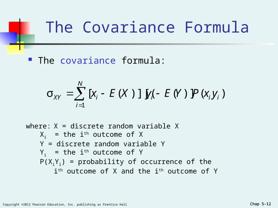
The Covariance Formula
The covariance formula:
)()]()][(([σ1
N
iiiiiXY yxPYEyXEx
where: X = discrete random variable XXi = the ith outcome of XY = discrete random variable YYi = the ith outcome of YP(XiYi) = probability of occurrence of the
ith outcome of X and the ith outcome of Y

Chap 5-13Copyright ©2012 Pearson Education, Inc. publishing as Prentice Hall Chap 5-13
Investment ReturnsThe Mean
Consider the return per $1000 for two types of investments.
Economic ConditionProb.
Investment
Passive Fund X Aggressive Fund Y
0.2 Recession - $25 - $200
0.5 Stable Economy + $50 + $60
0.3 Expanding Economy + $100 + $350

Chap 5-14Copyright ©2012 Pearson Education, Inc. publishing as Prentice Hall Chap 5-14
Investment ReturnsThe Mean
E(X) = μX = (-25)(.2) +(50)(.5) + (100)(.3) = 50
E(Y) = μY = (-200)(.2) +(60)(.5) + (350)(.3) = 95
Interpretation: Fund X is averaging a $50.00 return and fund Y is averaging a $95.00 return per $1000 invested.
Chap 5-15Copyright ©2012 Pearson Education, Inc. publishing as Prentice Hall Chap 5-15
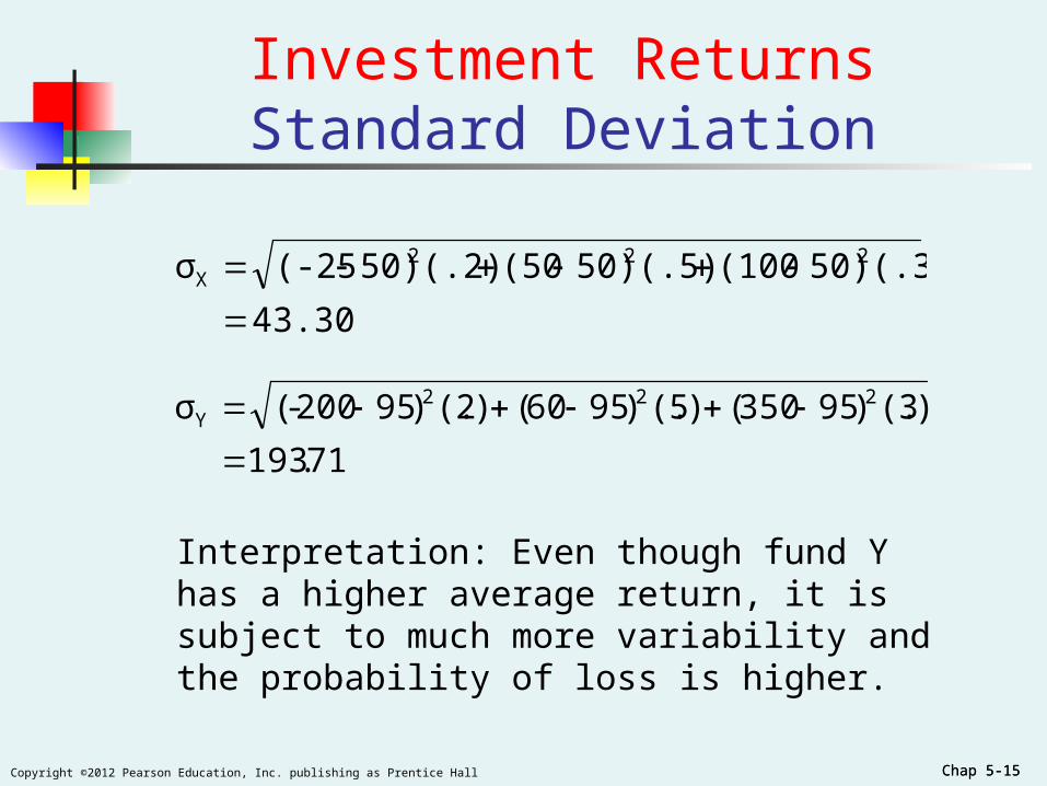
Investment ReturnsStandard Deviation
43.30
(.3)50)(100(.5)50)(50(.2)50)(-25σ 222X
71.193
)3(.)95350()5(.)9560()2(.)95200-(σ 222Y
Interpretation: Even though fund Y has a higher average return, it is subject to much more variability and the probability of loss is higher.
Chap 5-16Copyright ©2012 Pearson Education, Inc. publishing as Prentice Hall Chap 5-16
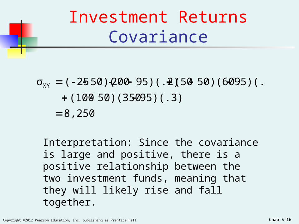
Investment ReturnsCovariance
8,250
95)(.3)50)(350(100
95)(.5)50)(60(5095)(.2)200-50)((-25σXY
Interpretation: Since the covariance is large and positive, there is a positive relationship between the two investment funds, meaning that they will likely rise and fall together.

Chap 5-17Copyright ©2012 Pearson Education, Inc. publishing as Prentice Hall Chap 5-17
The Sum of Two Random Variables
Expected Value of the sum of two random variables:
Variance of the sum of two random variables:
Standard deviation of the sum of two random variables:
XY2Y
2X
2YX σ2σσσY)Var(X
)Y(E)X(EY)E(X
2YXYX σσ
Chap 5-18Copyright ©2012 Pearson Education, Inc. publishing as Prentice Hall Chap 5-18
Portfolio Expected Return and Expected Risk
Investment portfolios usually contain several different funds (random variables)
The expected return and standard deviation of two funds together can now be calculated.
Investment Objective: Maximize return (mean) while minimizing risk (standard deviation).

Chap 5-19Copyright ©2012 Pearson Education, Inc. publishing as Prentice Hall Chap 5-19
Portfolio Expected Return and Portfolio Risk
Portfolio expected return (weighted average return):
Portfolio risk (weighted variability)
Where w = proportion of portfolio value in asset X
(1 - w) = proportion of portfolio value in asset Y
)Y(E)w1()X(EwE(P)
XY2Y
22X
2P w)σ-2w(1σ)w1(σwσ
Chap 5-20Copyright ©2012 Pearson Education, Inc. publishing as Prentice Hall Chap 5-20
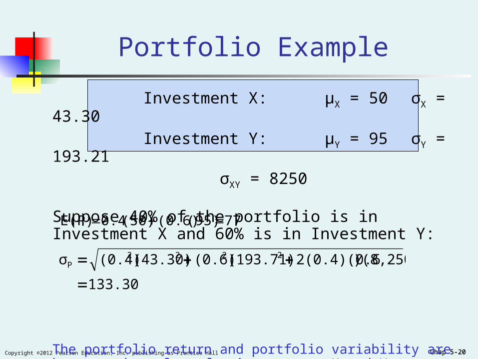
Portfolio Example
Investment X: μX = 50 σX = 43.30
Investment Y: μY = 95 σY = 193.21
σXY = 8250
Suppose 40% of the portfolio is in Investment X and 60% is in Investment Y:
The portfolio return and portfolio variability are between the values for investments X and Y considered individually
77(95)(0.6)(50)0.4E(P)
133.30
)(8,250)2(0.4)(0.6(193.71)(0.6)(43.30)(0.4)σ 2222P

Chap 5-21Copyright ©2012 Pearson Education, Inc. publishing as Prentice Hall Chap 5-21
Probability Distributions
Continuous Probability
Distributions
Binomial
Hypergeometric
Poisson
Probability Distributions
Discrete Probability
Distributions
Normal
Uniform
Exponential
Ch. 5 Ch. 6
Chap 5-22Copyright ©2012 Pearson Education, Inc. publishing as Prentice Hall Chap 5-22
Binomial Probability Distribution
A fixed number of observations, n e.g., 15 tosses of a coin; ten light bulbs taken from a warehouse
Each observation is categorized as to whether or not the “event of interest” occurred
e.g., head or tail in each toss of a coin; defective or not defective light bulb
Since these two categories are mutually exclusive and collectively exhaustive
When the probability of the event of interest is represented as π, then the probability of the event of interest not occurring is 1 - π
Constant probability for the event of interest occurring (π) for each observation
Probability of getting a tail is the same each time we toss the coin

Chap 5-23Copyright ©2012 Pearson Education, Inc. publishing as Prentice Hall Chap 5-23
Binomial Probability Distribution(continued)
Observations are independent The outcome of one observation does not affect the
outcome of the other Two sampling methods deliver independence
Infinite population without replacement Finite population with replacement
Chap 5-24Copyright ©2012 Pearson Education, Inc. publishing as Prentice Hall Chap 5-24
Possible Applications for the Binomial Distribution
A manufacturing plant labels items as either defective or acceptable
A firm bidding for contracts will either get a contract or not
A marketing research firm receives survey responses of “yes I will buy” or “no I will not”
New job applicants either accept the offer or reject it
Chap 5-25Copyright ©2012 Pearson Education, Inc. publishing as Prentice Hall Chap 5-25
The Binomial DistributionCounting Techniques
Suppose the event of interest is obtaining heads on the toss of a fair coin. You are to toss the coin three times. In how many ways can you get two heads?
Possible ways: HHT, HTH, THH, so there are three ways you can getting two heads.
This situation is fairly simple. We need to be able to count the number of ways for more complicated situations.
Chap 5-26Copyright ©2012 Pearson Education, Inc. publishing as Prentice Hall Chap 5-26
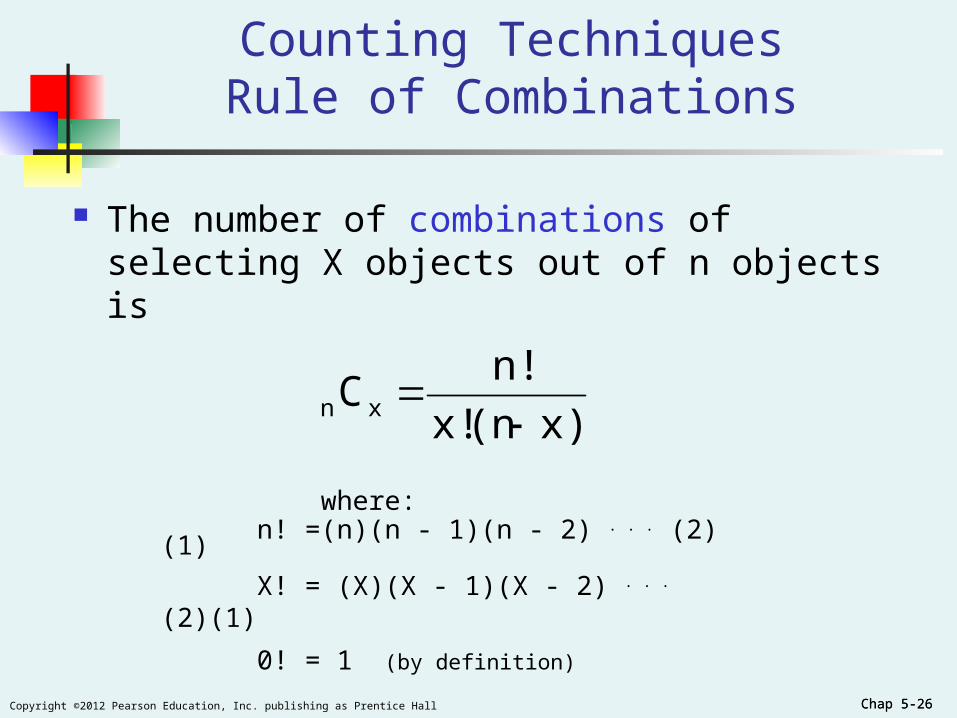
Counting TechniquesRule of Combinations
The number of combinations of selecting X objects out of n objects is
x)!(nx!
n!Cxn
where:n! =(n)(n - 1)(n - 2) . . . (2)(1)
X! = (X)(X - 1)(X - 2) . . . (2)(1)
0! = 1 (by definition)
Chap 5-27Copyright ©2012 Pearson Education, Inc. publishing as Prentice Hall Chap 5-27
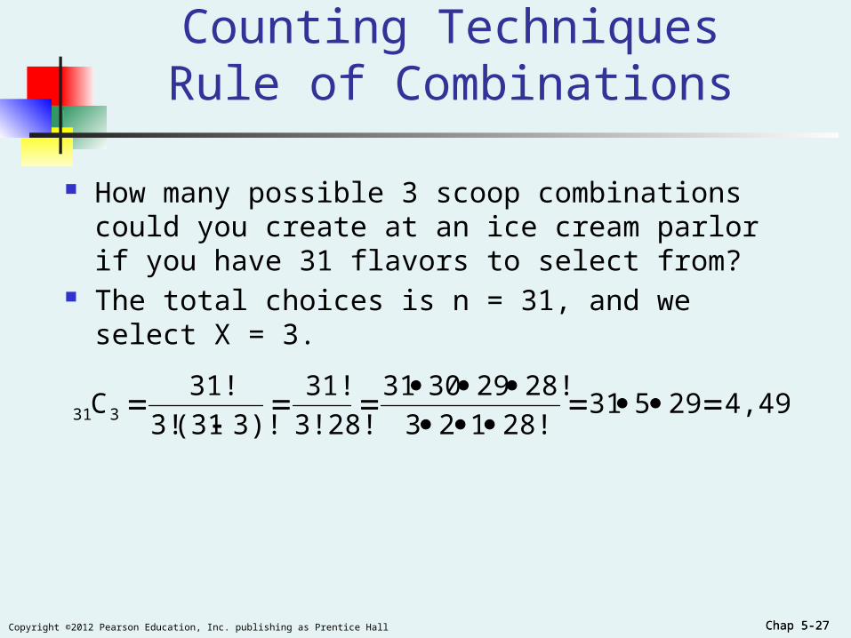
Counting TechniquesRule of Combinations
How many possible 3 scoop combinations could you create at an ice cream parlor if you have 31 flavors to select from?
The total choices is n = 31, and we select X = 3.
4,4952953128!123
28!293031
3!28!
31!
3)!(313!
31!C331

Chap 5-28Copyright ©2012 Pearson Education, Inc. publishing as Prentice Hall Chap 5-28
P(X=x|n,π) = probability of x events of interest in n trials, with the probability of
an “event of interest” being π for each trial
x = number of “events of interest” in sample, (x = 0, 1, 2, ..., n)
n = sample size (number of trials or
observations) π = probability of “event of interest”
P(X=x |n,π)n
x! n xπ (1-π)x n x!
( )!=
--
Example: Flip a coin four times, let x = # heads:
n = 4
π = 0.5
1 - π = (1 - 0.5) = 0.5
X = 0, 1, 2, 3, 4
Binomial Distribution Formula
Chap 5-29Copyright ©2012 Pearson Education, Inc. publishing as Prentice Hall Chap 5-29
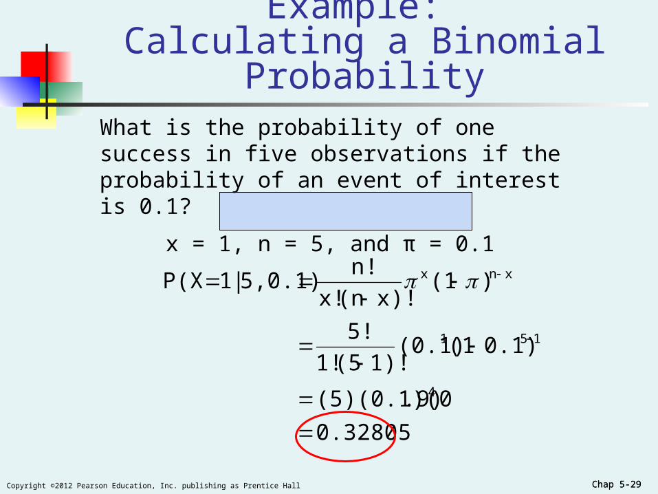
Example: Calculating a Binomial ProbabilityWhat is the probability of one success in five observations if the probability of an event of interest is 0.1?
x = 1, n = 5, and π = 0.1
0.32805
.9)(5)(0.1)(0
0.1)(1(0.1)1)!(51!
5!
)(1x)!(nx!
n!5,0.1)|1P(X
4
151
xnx

Chap 5-30Copyright ©2012 Pearson Education, Inc. publishing as Prentice Hall Chap 5-30
The Binomial DistributionExample
Suppose the probability of purchasing a defective computer is 0.02. What is the probability of purchasing 2 defective computers in a group of 10?
x = 2, n = 10, and π = 0.02
.01531
)(.8508)(45)(.0004
.02)(1(.02)2)!(102!
10!
)(1x)!(nx!
n!0.02) 10,|2P(X
2102
xnx

Chap 5-31Copyright ©2012 Pearson Education, Inc. publishing as Prentice Hall Chap 5-31
The Binomial DistributionShape
0.2.4.6
0 1 2 3 4 5 x
P(X=x|5, 0.1)
.2
.4
.6
0 1 2 3 4 5 x
P(X=x|5, 0.5)
0
The shape of the binomial distribution depends on the values of π and n
Here, n = 5 and π = .1
Here, n = 5 and π = .5

Chap 5-32Copyright ©2012 Pearson Education, Inc. publishing as Prentice Hall Chap 5-32
The Binomial Distribution Using Binomial Tables (Available On Line)
n = 10
x … π=.20 π=.25 π=.30 π=.35 π=.40 π=.45 π=.50
0123456789
10
……………………………
0.1074
0.2684
0.3020
0.2013
0.0881
0.0264
0.0055
0.0008
0.0001
0.0000
0.0000
0.0563
0.1877
0.2816
0.2503
0.1460
0.0584
0.0162
0.0031
0.0004
0.0000
0.0000
0.0282
0.12110.233
50.266
80.200
10.102
90.036
80.009
00.001
40.000
10.000
0
0.0135
0.0725
0.1757
0.2522
0.2377
0.1536
0.0689
0.0212
0.0043
0.0005
0.0000
0.0060
0.0403
0.1209
0.2150
0.2508
0.2007
0.11150.042
50.010
60.001
60.000
1
0.0025
0.0207
0.0763
0.1665
0.2384
0.2340
0.1596
0.0746
0.0229
0.0042
0.0003
0.00100.00980.04390.11720.20510.24610.20510.11720.04390.00980.0010
109876543210
… π=.80 π=.75 π=.70 π=.65 π=.60 π=.55 π=.50 x
Examples: n = 10, π = 0.35, x = 3: P(X = 3|10, 0.35) = 0.2522
n = 10, π = 0.75, x = 8: P(X = 2|10, 0.75) = 0.0004

Chap 5-33Copyright ©2012 Pearson Education, Inc. publishing as Prentice Hall Chap 5-33
Binomial Distribution Characteristics
Mean
Variance and Standard Deviation
nE(X)μ
)-(1nσ2 ππ
)-(1nσ ππWhere n = sample size
π = probability of the event of interest for any trial
(1 – π) = probability of no event of interest for any trial

Chap 5-34Copyright ©2012 Pearson Education, Inc. publishing as Prentice Hall Chap 5-34
The Binomial DistributionCharacteristics
0.2.4.6
0 1 2 3 4 5 x
P(X=x|5, 0.1)
.2
.4
.6
0 1 2 3 4 5 x
P(X=x|5, 0.5)
0
0.5(5)(.1)nμ π
0.6708
.1)(5)(.1)(1)-(1nσ
ππ
2.5(5)(.5)nμ π
1.118
.5)(5)(.5)(1)-(1nσ
ππ
Examples

Chap 5-35Copyright ©2012 Pearson Education, Inc. publishing as Prentice Hall Chap 5-35
Using Excel For TheBinomial Distribution (n = 4, π = 0.1)

Chap 5-36Copyright ©2012 Pearson Education, Inc. publishing as Prentice Hall
Using Minitab For The Binomial Distribution (n = 4, π = 0.1)
Chap 5-36
1
2
3
45
Chap 5-37Copyright ©2012 Pearson Education, Inc. publishing as Prentice Hall Chap 5-37
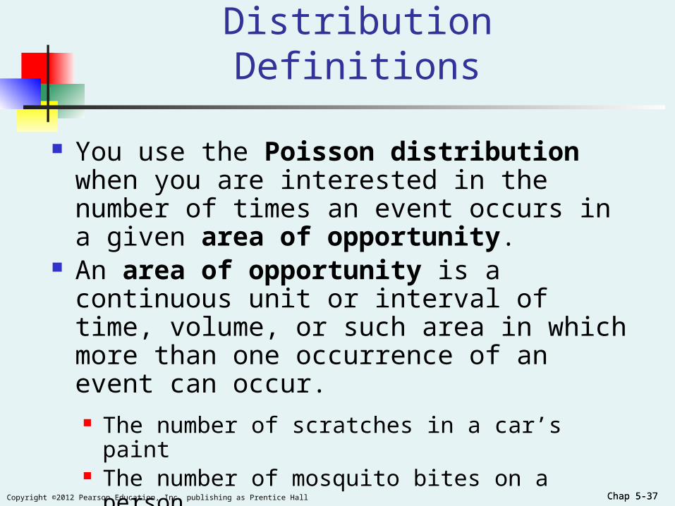
The Poisson DistributionDefinitions
You use the Poisson distribution when you are interested in the number of times an event occurs in a given area of opportunity.
An area of opportunity is a continuous unit or interval of time, volume, or such area in which more than one occurrence of an event can occur. The number of scratches in a car’s paint The number of mosquito bites on a person The number of computer crashes in a day
Chap 5-38Copyright ©2012 Pearson Education, Inc. publishing as Prentice Hall Chap 5-38
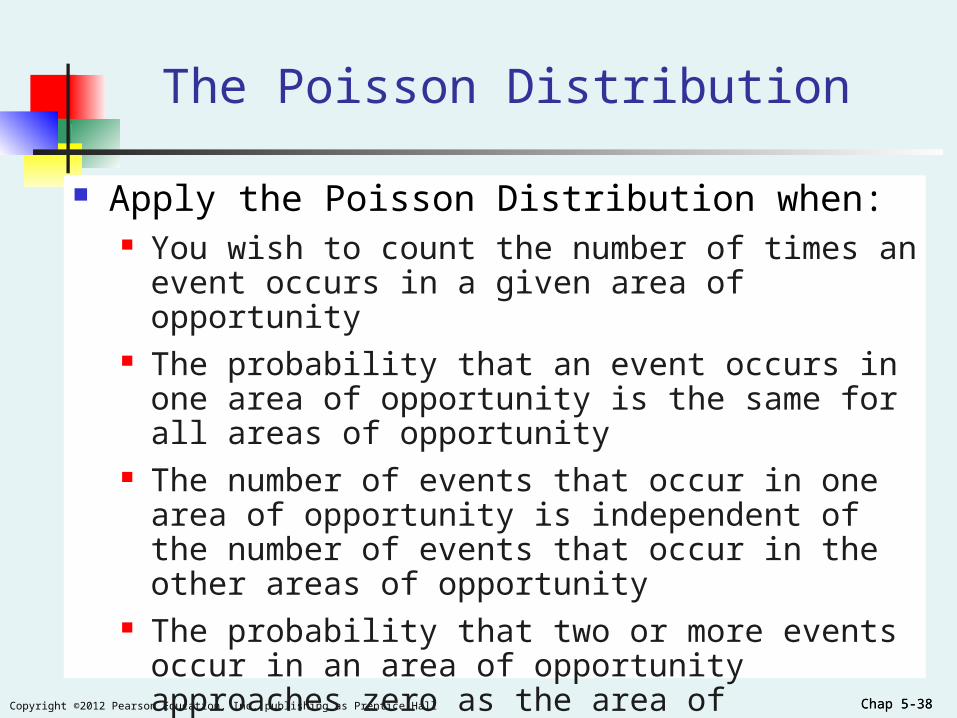
The Poisson Distribution
Apply the Poisson Distribution when: You wish to count the number of times an event
occurs in a given area of opportunity The probability that an event occurs in one area of
opportunity is the same for all areas of opportunity The number of events that occur in one area of
opportunity is independent of the number of events that occur in the other areas of opportunity
The probability that two or more events occur in an area of opportunity approaches zero as the area of opportunity becomes smaller
The average number of events per unit is (lambda)

Chap 5-39Copyright ©2012 Pearson Education, Inc. publishing as Prentice Hall Chap 5-39
Poisson Distribution Formula
where:
x = number of events in an area of opportunity
= expected number of events
e = base of the natural logarithm system (2.71828...)
!)|(
x
exXP
x
Chap 5-40Copyright ©2012 Pearson Education, Inc. publishing as Prentice Hall Chap 5-40
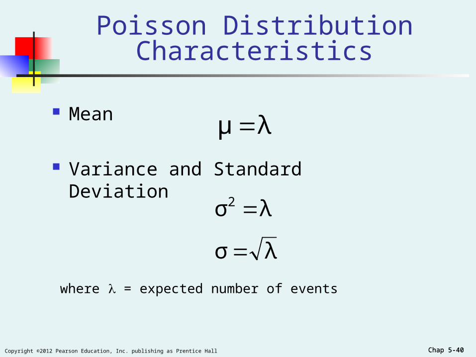
Poisson Distribution Characteristics
Mean
Variance and Standard Deviation
λμ
λσ2
λσ
where = expected number of events
Chap 5-41Copyright ©2012 Pearson Education, Inc. publishing as Prentice Hall Chap 5-41
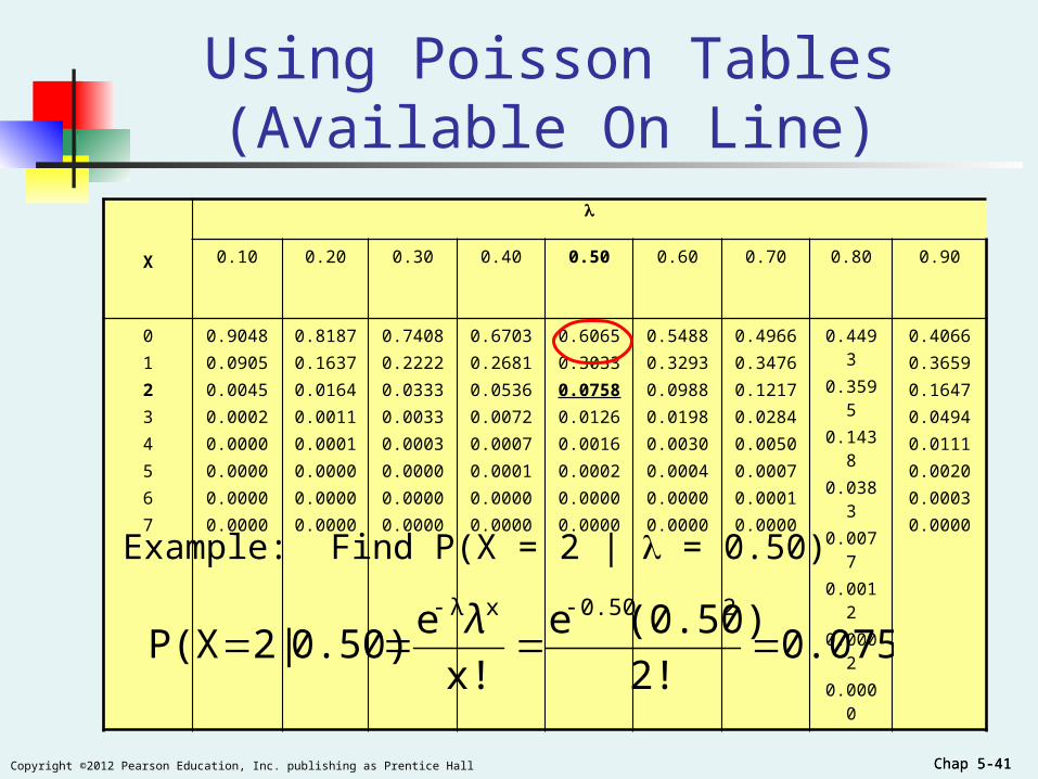
Using Poisson Tables (Available On Line)
X
0.10 0.20 0.30 0.40 0.50 0.60 0.70 0.80 0.90
01234567
0.90480.09050.00450.00020.00000.00000.00000.0000
0.81870.16370.01640.00110.00010.00000.00000.0000
0.74080.22220.03330.00330.00030.00000.00000.0000
0.67030.26810.05360.00720.00070.00010.00000.0000
0.60650.30330.07580.01260.00160.00020.00000.0000
0.54880.32930.09880.01980.00300.00040.00000.0000
0.49660.34760.12170.02840.00500.00070.00010.0000
0.44930.35950.14380.03830.00770.00120.00020.0000
0.40660.36590.16470.04940.01110.00200.00030.0000
Example: Find P(X = 2 | = 0.50)
0.07582!
(0.50)e
x!
e0.50) | 2P(X
20.50xλ
λ

Chap 5-42Copyright ©2012 Pearson Education, Inc. publishing as Prentice Hall Chap 5-42
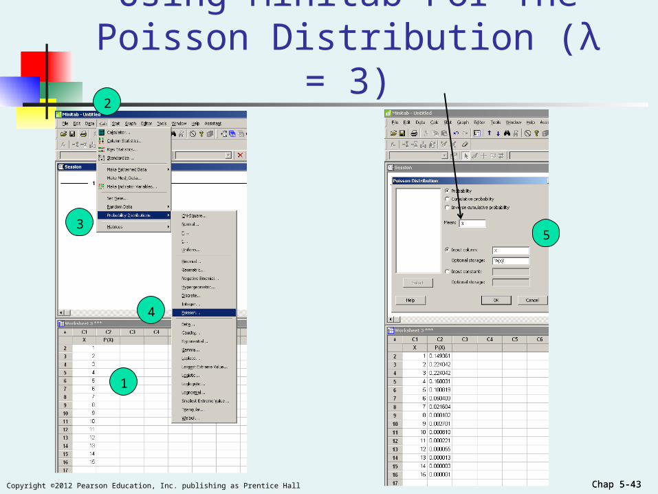
Using Excel For ThePoisson Distribution (λ= 3)
Chap 5-43Copyright ©2012 Pearson Education, Inc. publishing as Prentice Hall
Using Minitab For The Poisson Distribution (λ = 3)
Chap 5-43
1
2
3
4
5

Chap 5-44Copyright ©2012 Pearson Education, Inc. publishing as Prentice Hall Chap 5-44
Graph of Poisson Probabilities
X =
0.50
01234567
0.60650.30330.07580.01260.00160.00020.00000.0000 P(X = 2 | =0.50) = 0.0758
Graphically:
= 0.50

Chap 5-45Copyright ©2012 Pearson Education, Inc. publishing as Prentice Hall Chap 5-45
Poisson Distribution Shape
The shape of the Poisson Distribution depends on the parameter :
= 0.50 = 3.00
Chap 5-46Copyright ©2012 Pearson Education, Inc. publishing as Prentice Hall Chap 5-46
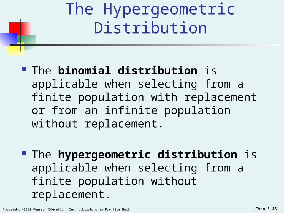
The Hypergeometric Distribution
The binomial distribution is applicable when selecting from a finite population with replacement or from an infinite population without replacement.
The hypergeometric distribution is applicable when selecting from a finite population without replacement.

Chap 5-47Copyright ©2012 Pearson Education, Inc. publishing as Prentice Hall Chap 5-47
The Hypergeometric Distribution
“n” trials in a sample taken from a finite population of size N
Sample taken without replacement
Outcomes of trials are dependent
Concerned with finding the probability of “X=xi”
items of interest in the sample where there are “A” items of interest in the population

Chap 5-48Copyright ©2012 Pearson Education, Inc. publishing as Prentice Hall Chap 5-48
Hypergeometric Distribution Formula
n
N
xn
AN
x
A
C
]C][C[A)N,n,|xP(X
nN
xnANxA
WhereN = population sizeA = number of items of interest in the population
N – A = number of events not of interest in the populationn = sample sizex = number of items of interest in the sample
n – x = number of events not of interest in the sample

Chap 5-49Copyright ©2012 Pearson Education, Inc. publishing as Prentice Hall Chap 5-49
Properties of the Hypergeometric Distribution
The mean of the hypergeometric distribution is
The standard deviation is
Where is called the “Finite Population Correction Factor” used when sampling without replacement from a finite population
N
nAE(X)μ
1- N
n-N
N
A)-nA(Nσ
2
1- N
n-N

Chap 5-50Copyright ©2012 Pearson Education, Inc. publishing as Prentice Hall Chap 5-50
Using the Hypergeometric Distribution
■ Example: 3 different computers are selected from 10 in the department. 4 of the 10 computers have illegal software loaded. What is the probability that 2 of the 3 selected computers have illegal software loaded?
N = 10 n = 3 A = 4 x = 2
0.3120
(6)(6)
3
10
1
6
2
4
n
N
xn
AN
x
A
3,10,4)|2P(X
The probability that 2 of the 3 selected computers have illegal software loaded is 0.30, or 30%.
Chap 5-51Copyright ©2012 Pearson Education, Inc. publishing as Prentice Hall Chap 5-51
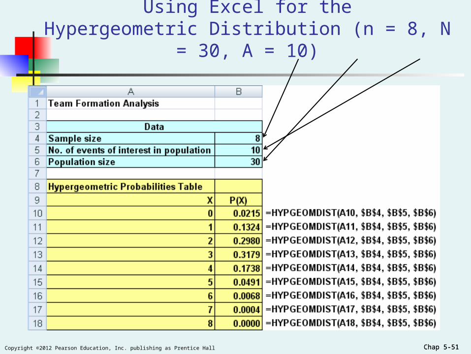
Using Excel for theHypergeometric Distribution (n = 8, N = 30, A = 10)
Chap 5-52Copyright ©2012 Pearson Education, Inc. publishing as Prentice Hall
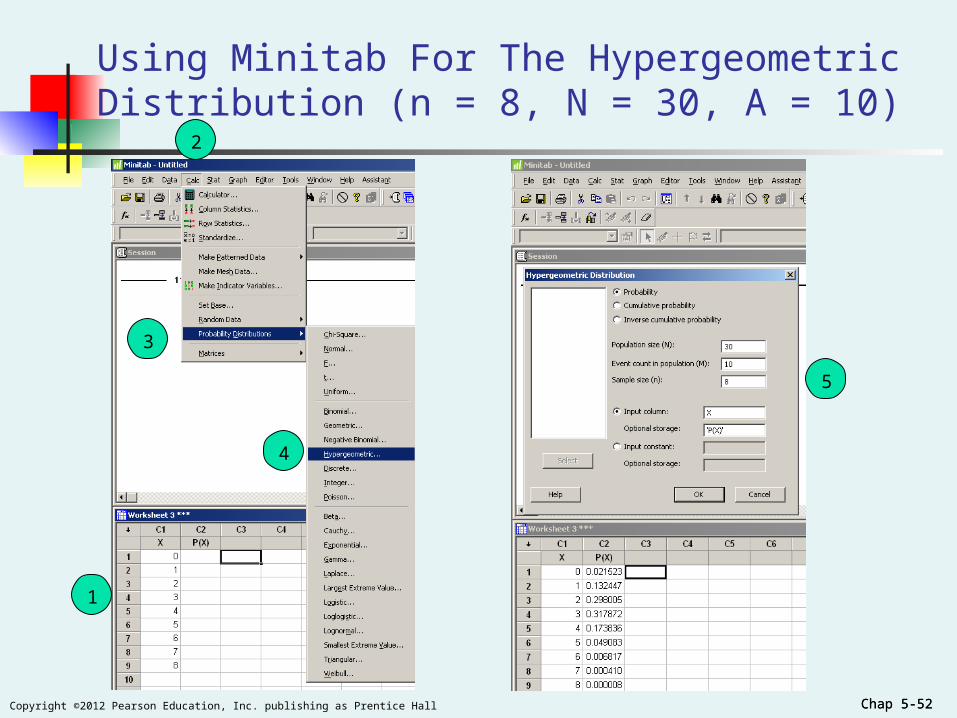
Using Minitab For The Hypergeometric Distribution (n = 8, N = 30, A = 10)
Chap 5-52
1
2
3
4
5

Chap 5-53Copyright ©2012 Pearson Education, Inc. publishing as Prentice Hall Chap 5-53
Chapter Summary
Addressed the probability distribution of a discrete random variable
Defined covariance and discussed its application in finance
Discussed the Binomial distribution Discussed the Poisson distribution Discussed the Hypergeometric distribution
Copyright ©2012 Pearson Education, Inc. publishing as Prentice Hall Chap 5-54
On Line Topic
The Poisson Approximation To The Binomial Distribution
Basic Business Statistics12th Edition
Chap 5-55Copyright ©2012 Pearson Education, Inc. publishing as Prentice Hall
Learning Objectives
In this topic, you learn: When to use the Poisson distribution to
approximate the binomial distribution How to use the Poisson distribution to approximate
the binomial distribution
Chap 5-56Copyright ©2012 Pearson Education, Inc. publishing as Prentice Hall
The Poisson Distribution Can Be Used To Approximate The Binomial Distribution
Most useful when n is large and π is very small
The approximation gets better as n gets larger and π gets smaller

Chap 5-57Copyright ©2012 Pearson Education, Inc. publishing as Prentice Hall
The Formula For The Approximation
!
)()(
X
neXP
Xn
WhereP(X) = probability of X events of interest given the parameters n and π n = sample size π = probability of an event of interest e = mathematical constant approximated by 2.71828 X = number of events of interest in the sample (X = 0, 1, 2, . . . , n)
Chap 5-58Copyright ©2012 Pearson Education, Inc. publishing as Prentice Hall
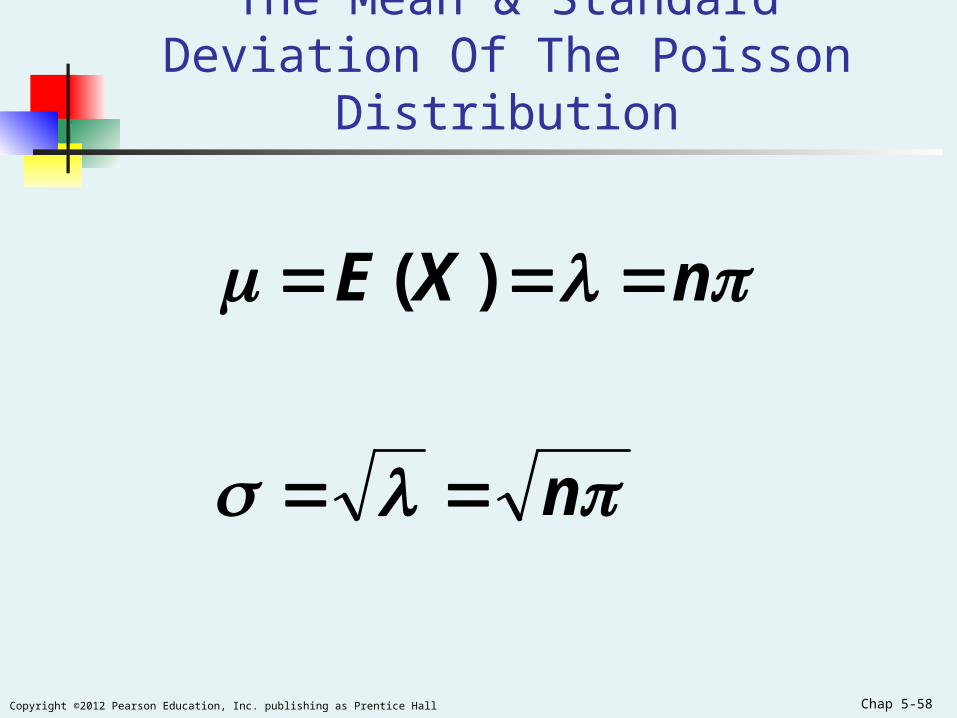
The Mean & Standard Deviation Of The Poisson Distribution
n
nXE
)(
Chap 5-59Copyright ©2012 Pearson Education, Inc. publishing as Prentice Hall
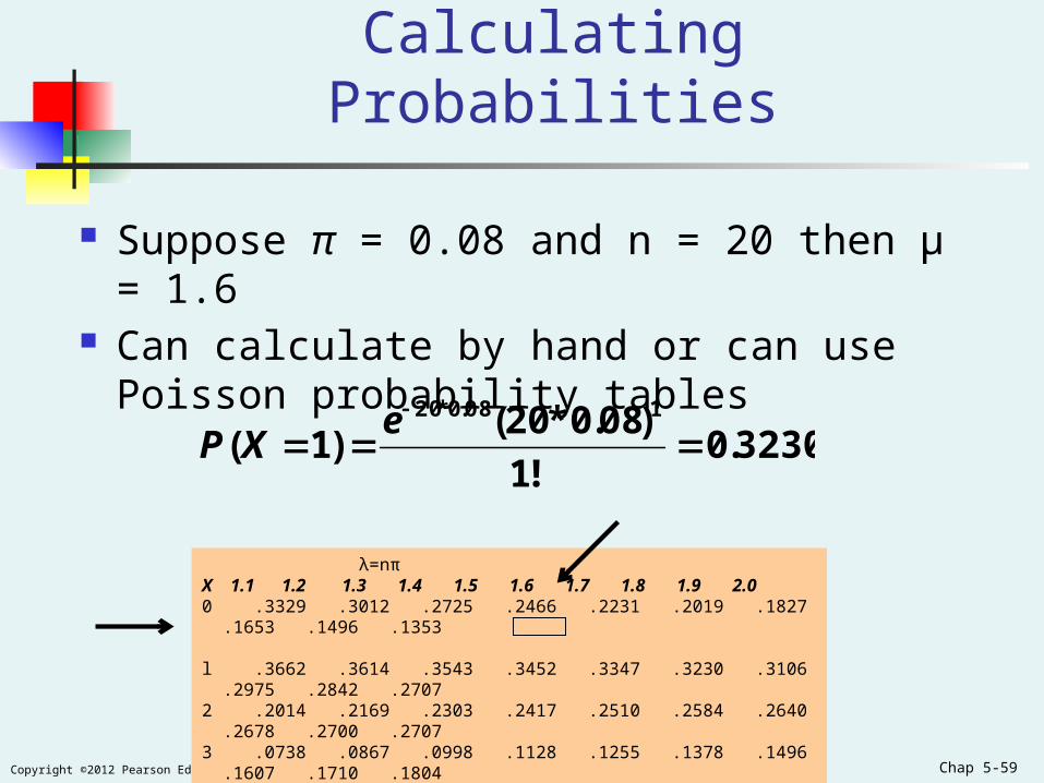
Calculating Probabilities
Suppose π = 0.08 and n = 20 then μ = 1.6 Can calculate by hand or can use Poisson
probability tables
λ=nπX 1.1 1.2 1.3 1.4 1.5 1.6 1.7 1.8 1.9 2.00 .3329 .3012 .2725 .2466 .2231 .2019 .1827 .1653 .1496 .1353 l .3662 .3614 .3543 .3452 .3347 .3230 .3106 .2975 .2842 .27072 .2014 .2169 .2303 .2417 .2510 .2584 .2640 .2678 .2700 .27073 .0738 .0867 .0998 .1128 .1255 .1378 .1496 .1607 .1710 .18044 .0203 .0260 .0324 .0395 .0471 .0551 .0636 .0723 .0812 .0902
3230.0!1
)08.0*20()1(
108.0*20
e
XP

Chap 5-60Copyright ©2012 Pearson Education, Inc. publishing as Prentice Hall
Topic Summary
In this topic, you learned: When to use the Poisson distribution to
approximate the binomial distribution How to use the Poisson distribution to approximate
the binomial distribution
Top Related