

![[PPT]Consumer Behavior and Marketing Strategy - Lars … to CB.ppt · Web viewIntro to Consumer Behavior Consumer behavior--what is it? Applications Consumer Behavior and Strategy](https://static.fdocuments.in/doc/165x107/5af357b67f8b9a74448b60fb/pptconsumer-behavior-and-marketing-strategy-lars-to-cbpptweb-viewintro.jpg)


Languages
Pages
Legal


個 體 經 濟 學 一 M i c r o e c o n o m i c s (I) *Untility function Total utility of consuming (x, y), denoted as u(x, y), is the total level of total satisfaction of consuming(x, y).
�Cardinal utility analysis (number itself is meaningful)
Ordinal utility analysis (number is used to rank bundles)�
In Ordinal utility analysis, higher value of TU is associated with higher level of satisfaction.
utility function is a function from bundles to a real number
such that � 𝑢(𝑥1,𝑦1) > 𝑢(𝑥2,𝑦2) (𝑥1,𝑦1) > (𝑥2,𝑦2)𝑢(𝑥1,𝑦1) = 𝑢(𝑥2,𝑦2) (𝑥1,𝑦1) ~ (𝑥2,𝑦2)
�
u : (x, y) → ℝ
EX: (2, 3) - 100 u(x, y) total utility (3, 7) - 130 (5, 10) - 200
*Marginal utility (of X, of Y) u = u(x, y)
MUx = ∆𝑢(𝑥,𝑦)∆𝑥
(𝜕𝑢(𝑥,𝑦)𝜕𝑥
)
MUy = ∆𝑢(𝑥,𝑦)∆𝑦
(𝜕𝑢(𝑥,𝑦)𝜕𝑦
)
The law of Diminishing marginal utility
x ↑ MUX↓ ( 𝜕2𝑢(𝑥,𝑦)𝜕𝑥2
< 0 )
y ↑ MUY↓ ( 𝜕2𝑢(𝑥,𝑦)𝜕𝑦2
< 0 )
CH2 The analysis of consumer behavior
Any positively monotonic transformation of a utility function is also a utility function representing the same preference. *Cardinal v.s. Ordinal utility analysis
EX: x : # of toast y: # of ham
u(x, y) = min �x3
, y2� positively monotonic
transformation→ min{x
3, y2}2 + 100
=> same preference. *Marginal utility
MUx = ∆u(x,y)∆x
MUy = ∆u(x,y)∆y
or ∂u(x,y)∂x
or ∂u(x,y)∂y
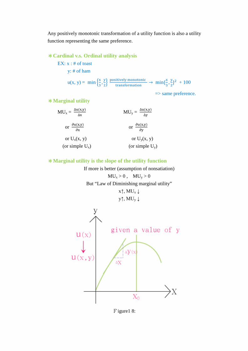
or Ux(x, y) or Uy(x, y) (or simple Ux) (or simple Uy) *Marginal utility is the slope of the utility function
If more is better (assumption of nonsatiation) MUx > 0 , MUy > 0
But “Law of Diminishing marginal utility” x↑, MUx ↓ y↑, MUy ↓
Figure1 8:
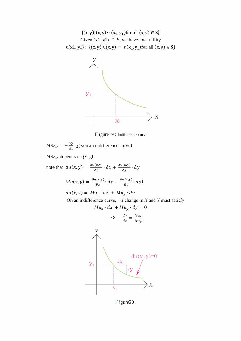
{(x, y)|(x, y)~ (x1, y1)for all (x, y) ∈ S} Given (x1, y1) ∈ S, we have total utility
u(x1, y1) : {(x, y)|u(x, y) = u(x1, y1)for all (x, y) ∈ S}
Figure19 : Indifference curve
MRSxy= −𝛥𝑦𝛥𝑥
(given an indifference curve)
MRSxy depends on (x, y)
note that ∆𝑢(𝑥, 𝑦) = ∆𝑢(𝑥,𝑦)∆𝑥
∙ ∆𝑥 + ∆𝑢(𝑥,𝑦)∆𝑦
∙ ∆𝑦
(𝑑𝑢(𝑥,𝑦) = 𝜕𝑢(𝑥,𝑦)𝜕𝑥
∙ 𝑑𝑥 + 𝜕𝑢(𝑥,𝑦)𝜕𝑦
∙ 𝑑𝑦)
𝑑𝑢(𝑥,𝑦) = 𝑀𝑢𝑥 ∙ 𝑑𝑥 + 𝑀𝑢𝑦 ∙ 𝑑𝑦 On an indifference curve, a change in X and Y must satisfy
𝑀𝑢𝑥 ∙ 𝑑𝑥 + 𝑀𝑢𝑦 ∙ 𝑑𝑦 = 0
−𝑑𝑦𝑑𝑥
= 𝑀𝑢𝑥𝑀𝑢𝑦
Figure20 :

(note: MRSxy= −𝛥𝑦𝛥𝑥
of an indifference curve)
MRSxy(x, y) = 𝑀𝑢𝑥(𝑥,𝑦)𝑀𝑢𝑦(𝑥,𝑦)
suppose������ 𝑀𝑢𝑥(𝑥,𝑦) is diminishing on 𝑋
𝑀𝑢𝑦(𝑥,𝑦) is diminishing on 𝑦 } Diminishing marginal utility.
Can we have diminishing MRSxy? (MRSxy↓ as x↑ or y↓)
x↑ => 𝑀𝑢𝑥↓(Diminishing 𝑀𝑢𝑥) y↓=> 𝑀𝑢𝑦↑(stays on the same IC)
Since MRSxy↓=𝑀𝑢𝑥↓𝑀𝑢𝑦↑
↓ as x↑
Figure21:Diminishing MRSxy
𝑑𝑀𝑅𝑆𝑥𝑦𝑑𝑥
>< 0 ?
We hope 𝑑𝑀𝑅𝑆𝑥𝑦𝑑𝑥
< 0.
Mux= ux Muy= uy
∆Mux(x,y)∆x
or ∂ux∂x
= uxx
∆Mux(x,y)∆y
or ∂ux∂y
= uxy
∆Muy(x,y)∆x
or ∂uy∂x
= uyx = uxy
∆Muy(x,y)∆y
or ∂uy∂y
= uyy

𝑑MRSxy𝑑x
=𝑑(Mux
Muy)
𝑑x=𝑑(ux
uy)
𝑑x=
uy𝑑𝑢𝑥𝑑x − ux
𝑑𝑢𝑦𝑑x
uy2
�note that duxdx
≠ ∂ux∂x� =
uy�∂ux∂x +
∂ux∂y ∙
dydx�−ux�
∂uy∂y +
∂ux∂y ∙
dydx�
uy2
a→c
∂ux∂x
(given y)
c→b ∂ux∂x
and dxdy
Figure22 :Diminishing MRSxy
(note that −dydx
= uxuy
(= MuxMuy
))
uy�uxx−uxy∙
uxuy�−ux�uyx−uyy∙
uxuy�
uy2
uy2�uxx−uxy∙
uxuy�−uxuy�uyx−uyy∙
uxuy�
uy3
uy2uxx−2uxuyuxy +ux2uyy
uy3< 0
none satisfaction ux,uy > 0 uxx<0uyy<0
} Diminishing Mux, Muy
Diminishing marginal utility is not sufficient to imply diminishing MRSxy, we need to know uxy >0<0

*Budget Constraint X, Y Quantity:x, y price: Px, Py income: m Expenditure of(x, y) = 𝑃𝑥 ∙ 𝑥 + 𝑃𝑦 ∙ 𝑦 Budget constraint: �(𝑥, 𝑦)�𝑃𝑥 ∙ 𝑥 + 𝑃𝑦 ∙ 𝑦 ≤ 𝑚� Budget line: �(𝑥,𝑦)�𝑃𝑥 ∙ 𝑥 + 𝑃𝑦 ∙ 𝑦 = 𝑚�
𝑃𝑥 ∙ 𝑥 + 𝑃𝑦 ∙ 𝑦 = 𝑚 𝑃𝑦 ∙ 𝑦 = 𝑚 − 𝑃𝑥 ∙ 𝑥
𝑦 =𝑚𝑃𝑦−𝑃𝑥 ∙ 𝑥𝑃𝑦
Figure23 :Budget constraint
𝑀𝑅𝑆𝑥𝑦 = −𝛥𝑦𝛥𝑥
|on an indifference curve = subject exchange rate.
𝑃𝑥𝑃𝑦
= −𝛥𝑦𝛥𝑥
|on an budget line = object exchange rate.
1. 所得(m)改變, m↑
Figure24 :Budget constraint when income change
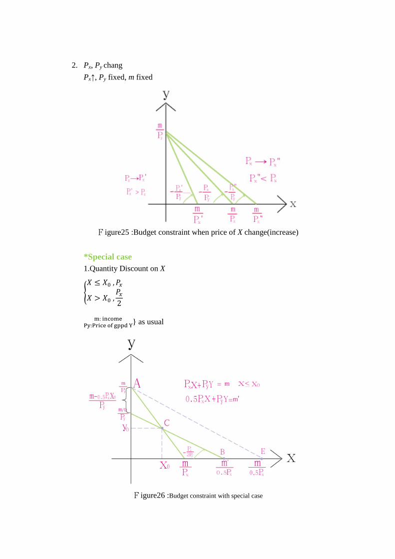
2. Px, Py chang
Px↑, Py fixed, m fixed
Figure25 :Budget constraint when price of X change(increase)
*Special case 1.Quantity Discount on X
�𝑋 ≤ 𝑋0 ,𝑃𝑥
𝑋 > 𝑋0 ,𝑃𝑥2�
m: incomePy:Price of gppd Y} as usual
Figure26 :Budget constraint with special case

𝑦0 =𝑚 − 𝑃𝑥𝑋0
𝑃𝑦
(x0, y0) is on D, B
Price of 𝑋 =0.5 𝑃𝑥 =𝑃𝑦
}on D, B
income = m’
0.5𝑃𝑥𝑋0 + 𝑃𝑦𝑚 − 𝑃𝑥𝑋0
𝑃𝑦= 𝑚′
0.5𝑃𝑥𝑋0 + 𝑚 − 𝑃𝑥𝑋0 = 𝑚′ 𝑚 − 0.5𝑃𝑥𝑋0 = 𝑚′ 𝑚 −𝑚′ = 0.5𝑃𝑥𝑋0
Distance between A.D=𝑚−0.5𝑃𝑥𝑋0𝑃𝑦
D.B budget line = �(𝑥,𝑦)�0.5𝑃𝑥𝑋 + 𝑃𝑦𝑌 = 𝑚 − 0.5𝑃𝑥𝑋0� X > X0
2.Quota on X
Figure27 :Budget constraint with quota
3. WIC(Woman.infant.children) Food coupon X0:good X of food coupon

Figure28 : Budget constraint with food coupon
4. Endowment 稟賦 (x0, y0)~m= Pxx0+Pyy0
Px↑, Px→Px’, Px’>Px m’ = Px’X0+PyY0
Figure29 :Budget constraint with endowment
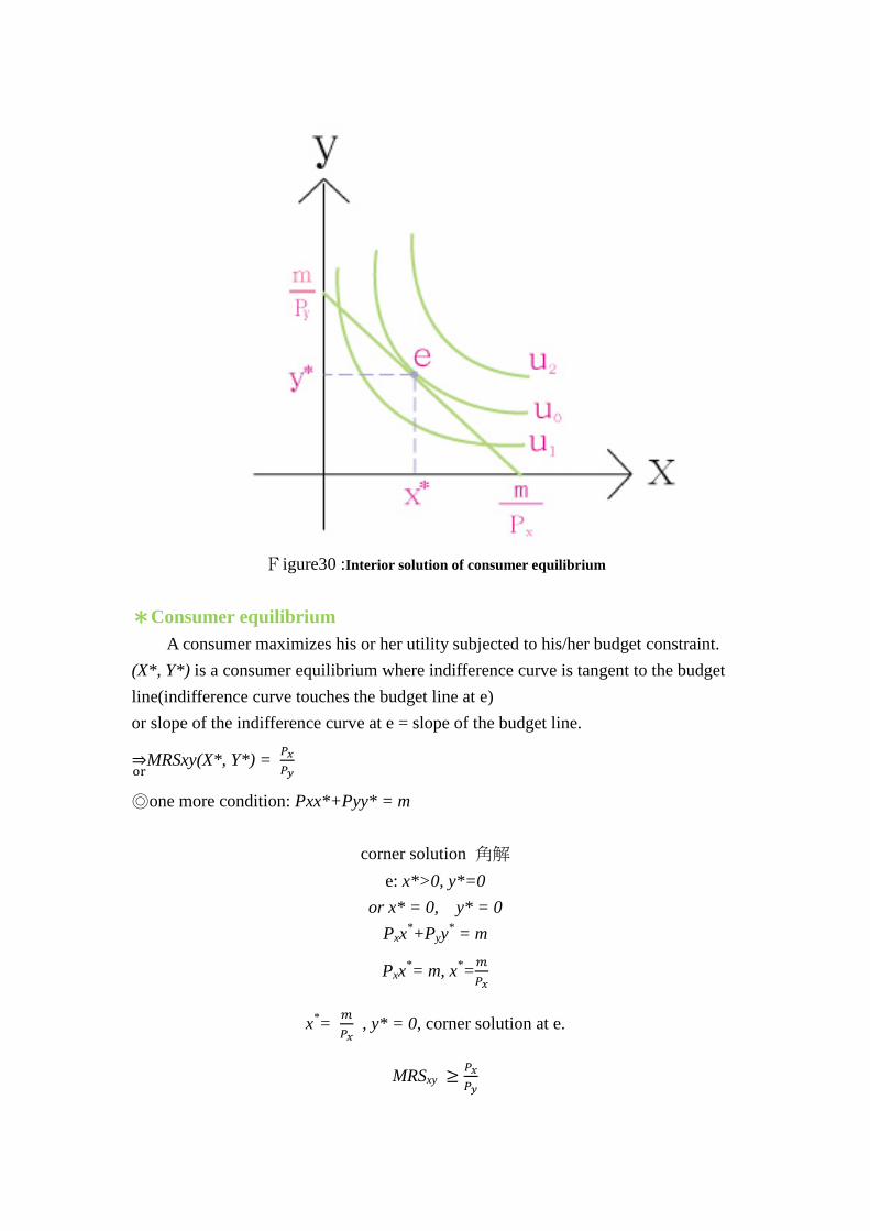
Figure30 :Interior solution of consumer equilibrium
*Consumer equilibrium A consumer maximizes his or her utility subjected to his/her budget constraint. (X*, Y*) is a consumer equilibrium where indifference curve is tangent to the budget line(indifference curve touches the budget line at e) or slope of the indifference curve at e = slope of the budget line.
or⇒MRSxy(X*, Y*) = 𝑃𝑥
𝑃𝑦
◎one more condition: Pxx*+Pyy* = m
corner solution 角解 e: x*>0, y*=0
or x* = 0, y* = 0 Pxx*+Pyy* = m
Pxx*= m, x*=𝑚𝑃𝑥
x*= 𝑚𝑃𝑥
, y* = 0, corner solution at e.
MRSxy ≥𝑃𝑥𝑃𝑦

Figure31 :Corner solution of consumer equilibrium
another corner solution:
x*= 0, y* = 𝑚𝑃𝑦
, MRSxy ≤𝑃𝑥𝑃𝑦
*In the interior solution case:
if MRSxy > 𝑃𝑥𝑃𝑦
subject change object exchange rate (主觀)個人偏好 (客觀)價錢比
x↑, y↓
Figure32 :
a→c c has more X => c is better than a. c→e
MRSxy = 𝑃𝑥𝑃𝑦
同理, MRSxy < 𝑃𝑥𝑃𝑦
=> x↓, y↑
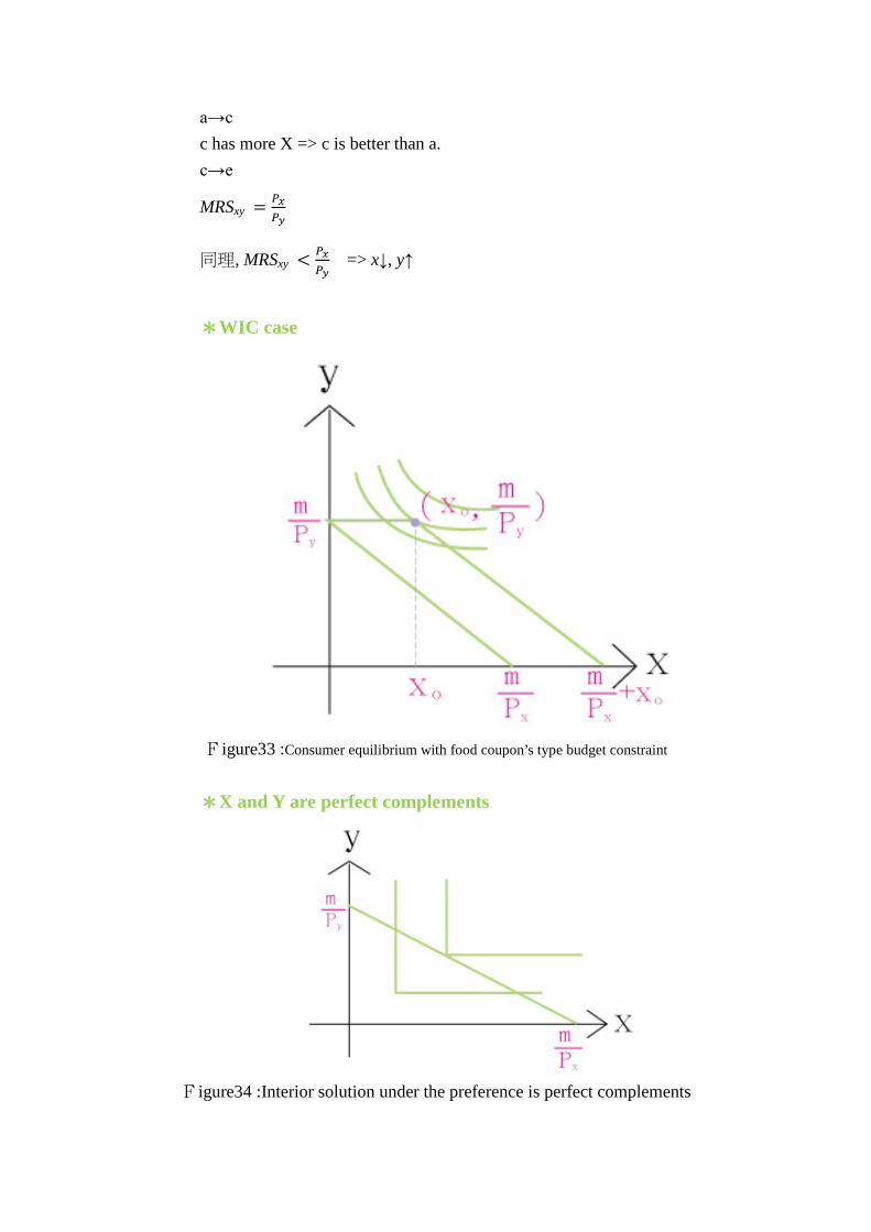
*WIC case
Figure33 :Consumer equilibrium with food coupon’s type budget constraint
*X and Y are perfect complements
Figure34 :Interior solution under the preference is perfect complements

*To max u(x, y) s.t 𝑷𝒙 ∙ 𝒙 + 𝑷𝒚 ∙ 𝒚 = 𝒎 u(x, y) is some continuously differentiable function How to solve the consumer’s problem? General problem: max f(x. y) s.t. g(x, y) = 0
(min) ℒ(𝑥,𝑦, 𝜆) = 𝑢(𝑥,𝑦) + 𝜆(𝑚− 𝑃𝑥𝑋 − 𝑃𝑦𝑌) …Lagrange multiplier method = 𝑓(𝑥,𝑦) + 𝜆𝑔(𝑥,𝑦) constrained problem →non-constrained problem and apply FOC to the
non- constrained problem.
○1 𝜕ℒ(𝑥,𝑦,𝜆)𝜕𝑥
=𝜕�𝑢(𝑥,𝑦)+𝜆�𝑚−𝑃𝑥𝑋−𝑃𝑦𝑌��
𝜕𝑥= 𝜕𝑢(𝑥,𝑦)
𝜕𝑥− 𝜆𝑃𝑥 = 0
𝜕𝑢(𝑥,𝑦)𝜕𝑥
= 𝜆𝑃𝑥 --○1 ’
○2 𝜕ℒ(𝑥,𝑦,𝜆)𝜕𝑦
=𝜕�𝑢(𝑥,𝑦)+𝜆�𝑚−𝑃𝑥𝑋−𝑃𝑦𝑌��
𝜕𝑦= 𝜕𝑢(𝑥,𝑦)
𝜕𝑦− 𝜆𝑃𝑦 = 0
𝜕𝑢(𝑥,𝑦)𝜕𝑦
= 𝜆𝑃𝑥 --○2 ’
○3 𝜕ℒ(𝑥,𝑦,𝜆)𝜕𝜆
=𝜕�𝑢(𝑥,𝑦)+𝜆�𝑚−𝑃𝑥𝑋−𝑃𝑦𝑌��
𝜕𝜆= 𝑚− 𝑃𝑥𝑥 − 𝑃𝑦𝑦 = 0 --○3 ’
budget constraint
○1 '/○2 '=𝑀𝑢𝑥𝑀𝑢𝑦
= 𝑃𝑥𝑃𝑦
--○4
MRSxy = 𝑀𝑢𝑥𝑀𝑢𝑦
○4 MRSxy = 𝑀𝑢𝑥𝑀𝑢𝑦
=𝑃𝑥𝑃𝑦
在同樣的$1 上比較
𝑀𝑢𝑥𝑃𝑥
= 𝑀𝑢𝑦𝑃𝑦
⇒ 𝑀𝑢𝑥𝑃𝑥
= ∆𝑢(𝑥,𝑦)∆𝑥
∆𝑒𝑥𝑝𝑒𝑛𝑑𝑖𝑡𝑢𝑟𝑒∆𝑥
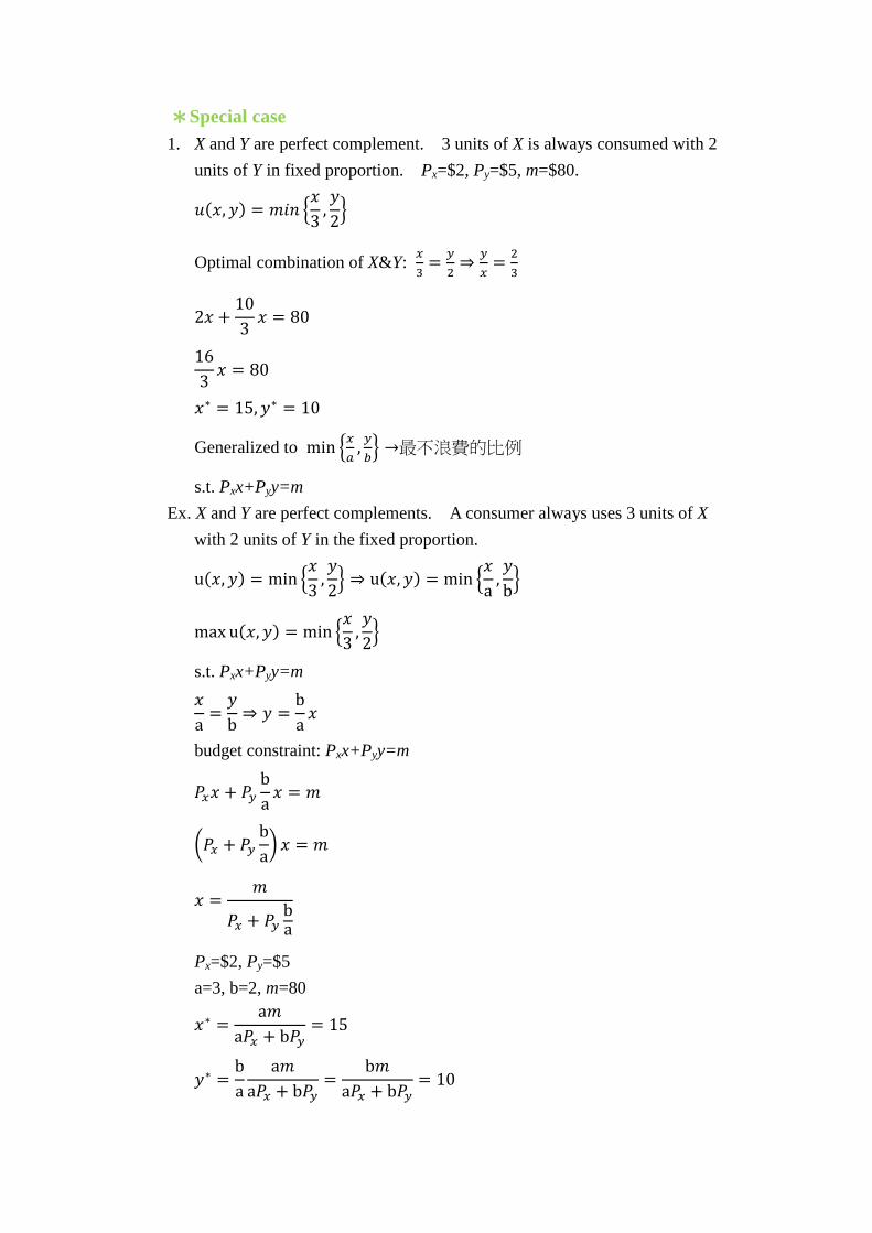
*Special case 1. X and Y are perfect complement. 3 units of X is always consumed with 2
units of Y in fixed proportion. Px=$2, Py=$5, m=$80.
𝑢(𝑥,𝑦) = 𝑚𝑖𝑛 �𝑥3
,𝑦2�
Optimal combination of X&Y: 𝑥3
= 𝑦2⇒ 𝑦
𝑥= 2
3
2𝑥 +103𝑥 = 80
163𝑥 = 80
𝑥∗ = 15,𝑦∗ = 10
Generalized to min �𝑥𝑎
, 𝑦𝑏� →最不浪費的比例
s.t. Pxx+Pyy=m Ex. X and Y are perfect complements. A consumer always uses 3 units of X
with 2 units of Y in the fixed proportion.
u(𝑥,𝑦) = min �𝑥3
,𝑦2� ⇒ u(𝑥,𝑦) = min �
𝑥a
,𝑦b�
max u(𝑥,𝑦) = min �𝑥3
,𝑦2�
s.t. Pxx+Pyy=m 𝑥a
=𝑦b⇒ 𝑦 =
ba𝑥
budget constraint: Pxx+Pyy=m
𝑃𝑥𝑥 + 𝑃𝑦ba𝑥 = 𝑚
�𝑃𝑥 + 𝑃𝑦ba� 𝑥 = 𝑚
𝑥 =𝑚
𝑃𝑥 + 𝑃𝑦ba
Px=$2, Py=$5 a=3, b=2, m=80
𝑥∗ =a𝑚
a𝑃𝑥 + b𝑃𝑦= 15
𝑦∗ =ba
a𝑚a𝑃𝑥 + b𝑃𝑦
=b𝑚
a𝑃𝑥 + b𝑃𝑦= 10
Ex. Cobb-Douglas utility function 𝑢(𝑥,𝑦)total utility = 𝑥α𝑦β, α, β > 0
𝑀𝑢𝑥 = ∂𝑢(𝑥,𝑦)∂𝑥
= ∂𝑥α𝑦β
∂𝑥= α𝑥α−1𝑦β > 0 no satiation point (no bliss point)
Muy = ∂u(x,y)∂y
= ∂xαyβ
∂y= βxαyβ−1 > 0
∂𝑀𝑢𝑥∂𝑥
= α(α− 1)𝑥α−2𝑦β ⇒ α < 1
𝜕𝑀𝑢𝑦𝜕𝑦
= 𝛽(𝛽 − 1)𝑥𝛼𝑦𝛽−2 ⇒ 𝛽 < 1 → 𝐷𝑖𝑚𝑖𝑛𝑖𝑠ℎ𝑖𝑛𝑔 𝑀𝑎𝑟𝑔𝑖𝑛𝑎𝑙 𝑢𝑡𝑖𝑙𝑖𝑡𝑦
𝑀𝑅𝑆𝑥𝑦 =𝑀𝑢𝑥𝑀𝑢𝑦
=𝛼𝑥𝛼−1𝑦𝛽
𝛽𝑥𝛼𝑦𝛽−1=𝛼𝛽𝑦𝑥→ �𝑥越大,𝑦越小� ⇒
𝑑𝑀𝑅𝑆𝑥𝑦𝑑𝑥
< 0
For any α, β>0 and for all x and y 𝑑𝑀𝑅𝑆𝑥𝑦𝑑𝑥
< 0
i.e. MRSxy is diminishing (with x) i.e. indifference curve is always convex
In equilibrium, 𝑀𝑅𝑆𝑥𝑦 = 𝑃𝑥𝑃𝑦
𝛼𝛽𝑦𝑥
=𝑃𝑥𝑃𝑦
𝑃𝑦𝑦(expenditure on Y) =𝛽 𝛼𝑃𝑥𝑥(expenditure on 𝑋)
𝑃𝑥𝑥 + 𝑃𝑦𝑦 = 𝑚
𝑃𝑥𝑥 +𝛽 𝛼𝑃𝑥𝑥 = 𝑚
𝛼 + 𝛽 𝛼
𝑃𝑥𝑥 = 𝑚⟹ 𝑒𝑥(expenditure of x) = 𝑃𝑥𝑥 =𝛼
𝛼 + 𝛽 𝑚(short of 𝑒𝑥)
𝑒𝑦(expenditure of y) = 𝑃𝑦𝑦 =𝛽
𝛼 + 𝛽 𝑚(short of 𝑒𝑦)
𝑥∗ =𝛼
𝛼 + 𝛽𝑚𝑃𝑥
𝑦∗ =𝛽
𝛼 + 𝛽𝑚𝑃𝑦
Top Related