
CH2 The analysis of consumer behavior
15
個 體 經 濟 學 一 M i c r o e c o n o m i c s (I) *Untility function Total utility of consuming (x, y), denoted as u(x, y), is the total level of total satisfaction of consuming(x, y). � Cardinal utility analysis (number itself is meaningful) Ordinal utility analysis (number is used to rank bundles) In Ordinal utility analysis, higher value of TU is associated with higher level of satisfaction. utility function is a function from bundles to a real number such that � (1, 1) > (2, 2) (1, 1) > (2, 2) (1, 1) = (2, 2) (1, 1) ~ (2, 2) u : (x, y) → ℝ EX: (2, 3) - 100 u(x, y) total utility (3, 7) - 130 (5, 10) - 200 *Marginal utility (of X, of Y) u = u(x, y) MU x = ∆(,) ∆ ( (,) ) MU y = ∆(,) ∆ ( (,) ) The law of Diminishing marginal utility x ↑ MU X ↓ ( 2 (,) 2 <0 ) y ↑ MU Y ↓ ( 2 (,) 2 <0 ) CH2 The analysis of consumer behavior
Transcript of CH2 The analysis of consumer behavior

個 體 經 濟 學 一 M i c r o e c o n o m i c s (I) *Untility function Total utility of consuming (x, y), denoted as u(x, y), is the total level of total satisfaction of consuming(x, y).
�Cardinal utility analysis (number itself is meaningful)
Ordinal utility analysis (number is used to rank bundles)�
In Ordinal utility analysis, higher value of TU is associated with higher level of satisfaction.
utility function is a function from bundles to a real number
such that � 𝑢(𝑥1,𝑦1) > 𝑢(𝑥2,𝑦2) (𝑥1,𝑦1) > (𝑥2,𝑦2)𝑢(𝑥1,𝑦1) = 𝑢(𝑥2,𝑦2) (𝑥1,𝑦1) ~ (𝑥2,𝑦2)
�
u : (x, y) → ℝ
EX: (2, 3) - 100 u(x, y) total utility (3, 7) - 130 (5, 10) - 200
*Marginal utility (of X, of Y) u = u(x, y)
MUx = ∆𝑢(𝑥,𝑦)∆𝑥
(𝜕𝑢(𝑥,𝑦)𝜕𝑥
)
MUy = ∆𝑢(𝑥,𝑦)∆𝑦
(𝜕𝑢(𝑥,𝑦)𝜕𝑦
)
The law of Diminishing marginal utility
x ↑ MUX↓ ( 𝜕2𝑢(𝑥,𝑦)𝜕𝑥2
< 0 )
y ↑ MUY↓ ( 𝜕2𝑢(𝑥,𝑦)𝜕𝑦2
< 0 )
CH2 The analysis of consumer behavior
Any positively monotonic transformation of a utility function is also a utility function representing the same preference. *Cardinal v.s. Ordinal utility analysis
EX: x : # of toast y: # of ham
u(x, y) = min �x3
, y2� positively monotonic
transformation→ min{x
3, y2}2 + 100
=> same preference. *Marginal utility
MUx = ∆u(x,y)∆x
MUy = ∆u(x,y)∆y
or ∂u(x,y)∂x
or ∂u(x,y)∂y
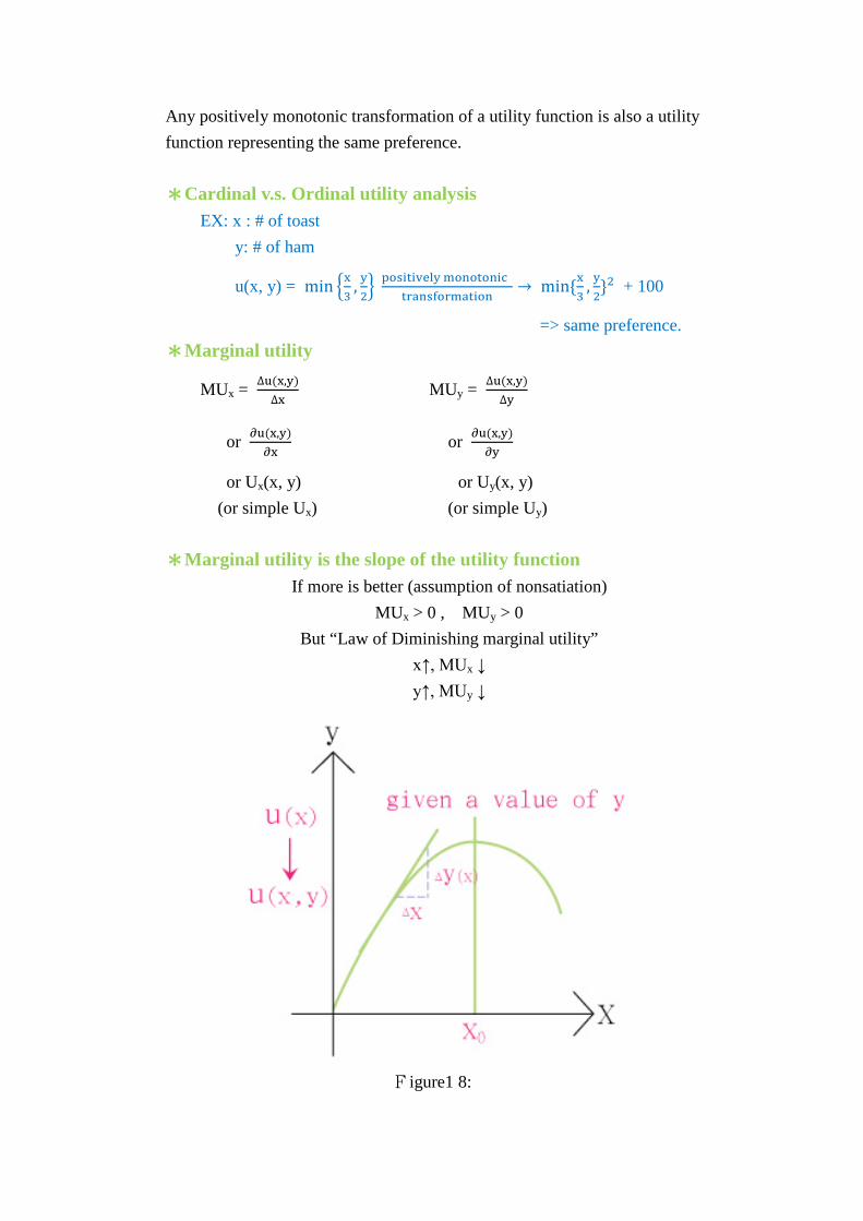
or Ux(x, y) or Uy(x, y) (or simple Ux) (or simple Uy) *Marginal utility is the slope of the utility function
If more is better (assumption of nonsatiation) MUx > 0 , MUy > 0
But “Law of Diminishing marginal utility” x↑, MUx ↓ y↑, MUy ↓
Figure1 8:
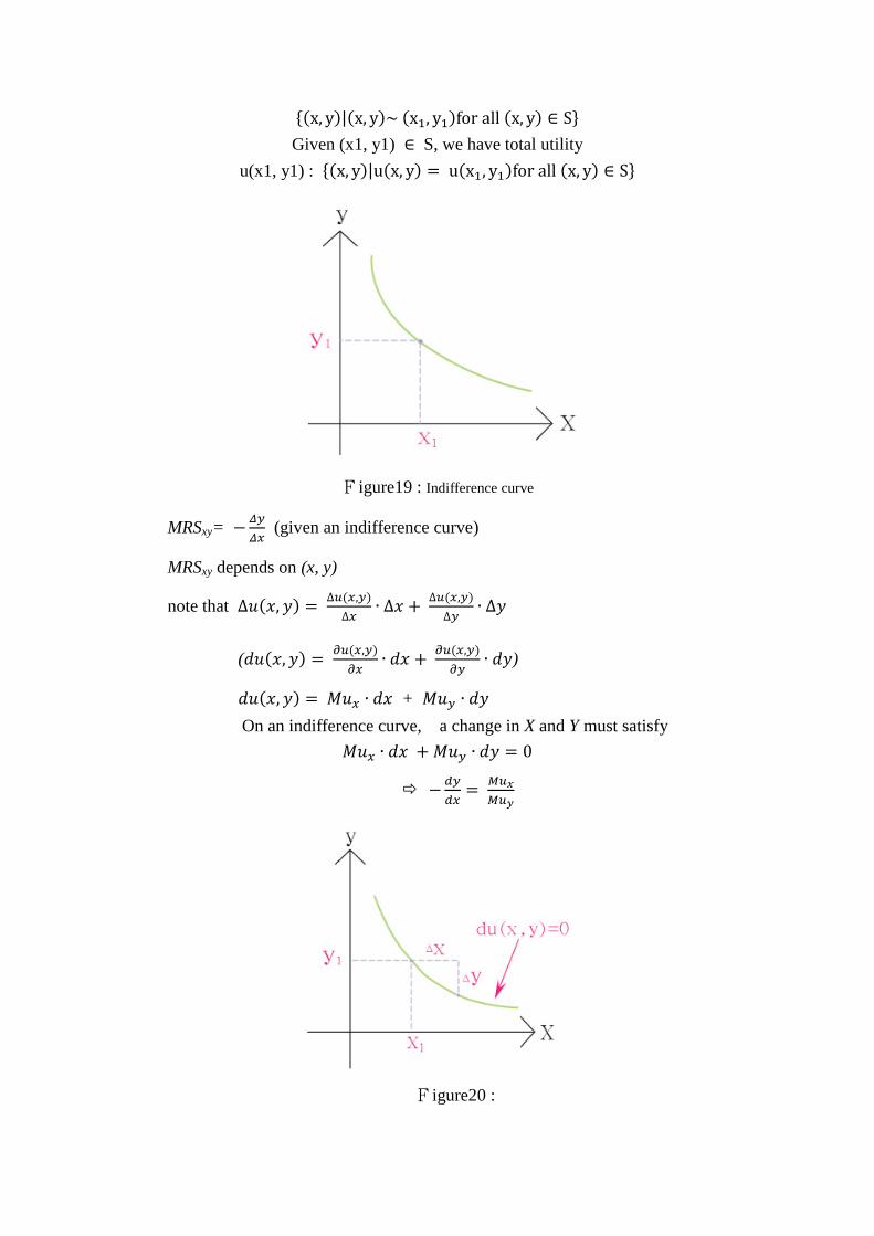
{(x, y)|(x, y)~ (x1, y1)for all (x, y) ∈ S} Given (x1, y1) ∈ S, we have total utility
u(x1, y1) : {(x, y)|u(x, y) = u(x1, y1)for all (x, y) ∈ S}
Figure19 : Indifference curve
MRSxy= −𝛥𝑦𝛥𝑥
(given an indifference curve)
MRSxy depends on (x, y)
note that ∆𝑢(𝑥, 𝑦) = ∆𝑢(𝑥,𝑦)∆𝑥
∙ ∆𝑥 + ∆𝑢(𝑥,𝑦)∆𝑦
∙ ∆𝑦
(𝑑𝑢(𝑥,𝑦) = 𝜕𝑢(𝑥,𝑦)𝜕𝑥
∙ 𝑑𝑥 + 𝜕𝑢(𝑥,𝑦)𝜕𝑦
∙ 𝑑𝑦)
𝑑𝑢(𝑥,𝑦) = 𝑀𝑢𝑥 ∙ 𝑑𝑥 + 𝑀𝑢𝑦 ∙ 𝑑𝑦 On an indifference curve, a change in X and Y must satisfy
𝑀𝑢𝑥 ∙ 𝑑𝑥 + 𝑀𝑢𝑦 ∙ 𝑑𝑦 = 0
−𝑑𝑦𝑑𝑥
= 𝑀𝑢𝑥𝑀𝑢𝑦
Figure20 :

(note: MRSxy= −𝛥𝑦𝛥𝑥
of an indifference curve)
MRSxy(x, y) = 𝑀𝑢𝑥(𝑥,𝑦)𝑀𝑢𝑦(𝑥,𝑦)
suppose������ 𝑀𝑢𝑥(𝑥,𝑦) is diminishing on 𝑋
𝑀𝑢𝑦(𝑥,𝑦) is diminishing on 𝑦 } Diminishing marginal utility.
Can we have diminishing MRSxy? (MRSxy↓ as x↑ or y↓)
x↑ => 𝑀𝑢𝑥↓(Diminishing 𝑀𝑢𝑥) y↓=> 𝑀𝑢𝑦↑(stays on the same IC)
Since MRSxy↓=𝑀𝑢𝑥↓𝑀𝑢𝑦↑
↓ as x↑
Figure21:Diminishing MRSxy
𝑑𝑀𝑅𝑆𝑥𝑦𝑑𝑥
>< 0 ?
We hope 𝑑𝑀𝑅𝑆𝑥𝑦𝑑𝑥
< 0.
Mux= ux Muy= uy
∆Mux(x,y)∆x
or ∂ux∂x
= uxx
∆Mux(x,y)∆y
or ∂ux∂y
= uxy
∆Muy(x,y)∆x
or ∂uy∂x
= uyx = uxy
∆Muy(x,y)∆y
or ∂uy∂y
= uyy

𝑑MRSxy𝑑x
=𝑑(Mux
Muy)
𝑑x=𝑑(ux
uy)
𝑑x=
uy𝑑𝑢𝑥𝑑x − ux
𝑑𝑢𝑦𝑑x
uy2
�note that duxdx
≠ ∂ux∂x� =
uy�∂ux∂x +
∂ux∂y ∙
dydx�−ux�
∂uy∂y +
∂ux∂y ∙
dydx�
uy2
a→c
∂ux∂x
(given y)
c→b ∂ux∂x
and dxdy
Figure22 :Diminishing MRSxy
(note that −dydx
= uxuy
(= MuxMuy
))
uy�uxx−uxy∙
uxuy�−ux�uyx−uyy∙
uxuy�
uy2
uy2�uxx−uxy∙
uxuy�−uxuy�uyx−uyy∙
uxuy�
uy3
uy2uxx−2uxuyuxy +ux2uyy
uy3< 0
none satisfaction ux,uy > 0 uxx<0uyy<0
} Diminishing Mux, Muy
Diminishing marginal utility is not sufficient to imply diminishing MRSxy, we need to know uxy >0<0

*Budget Constraint X, Y Quantity:x, y price: Px, Py income: m Expenditure of(x, y) = 𝑃𝑥 ∙ 𝑥 + 𝑃𝑦 ∙ 𝑦 Budget constraint: �(𝑥, 𝑦)�𝑃𝑥 ∙ 𝑥 + 𝑃𝑦 ∙ 𝑦 ≤ 𝑚� Budget line: �(𝑥,𝑦)�𝑃𝑥 ∙ 𝑥 + 𝑃𝑦 ∙ 𝑦 = 𝑚�
𝑃𝑥 ∙ 𝑥 + 𝑃𝑦 ∙ 𝑦 = 𝑚 𝑃𝑦 ∙ 𝑦 = 𝑚 − 𝑃𝑥 ∙ 𝑥
𝑦 =𝑚𝑃𝑦−𝑃𝑥 ∙ 𝑥𝑃𝑦
Figure23 :Budget constraint
𝑀𝑅𝑆𝑥𝑦 = −𝛥𝑦𝛥𝑥
|on an indifference curve = subject exchange rate.
𝑃𝑥𝑃𝑦
= −𝛥𝑦𝛥𝑥
|on an budget line = object exchange rate.
1. 所得(m)改變, m↑
Figure24 :Budget constraint when income change
2. Px, Py chang
Px↑, Py fixed, m fixed
Figure25 :Budget constraint when price of X change(increase)
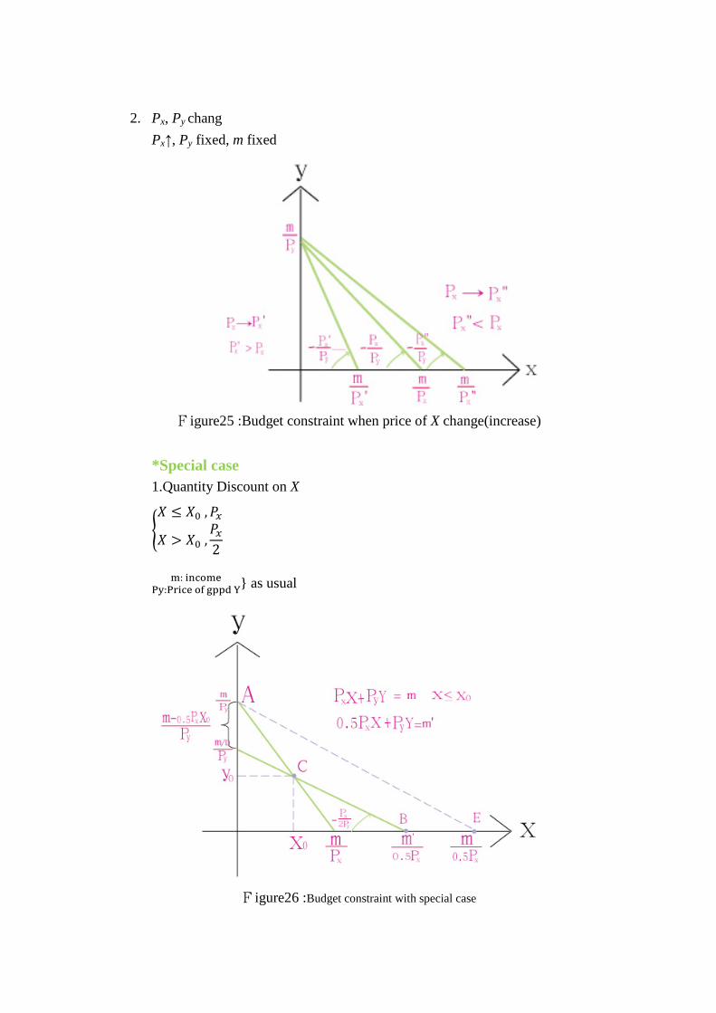
*Special case 1.Quantity Discount on X
�𝑋 ≤ 𝑋0 ,𝑃𝑥
𝑋 > 𝑋0 ,𝑃𝑥2�
m: incomePy:Price of gppd Y} as usual
Figure26 :Budget constraint with special case

𝑦0 =𝑚 − 𝑃𝑥𝑋0
𝑃𝑦
(x0, y0) is on D, B
Price of 𝑋 =0.5 𝑃𝑥 =𝑃𝑦
}on D, B
income = m’
0.5𝑃𝑥𝑋0 + 𝑃𝑦𝑚 − 𝑃𝑥𝑋0
𝑃𝑦= 𝑚′
0.5𝑃𝑥𝑋0 + 𝑚 − 𝑃𝑥𝑋0 = 𝑚′ 𝑚 − 0.5𝑃𝑥𝑋0 = 𝑚′ 𝑚 −𝑚′ = 0.5𝑃𝑥𝑋0
Distance between A.D=𝑚−0.5𝑃𝑥𝑋0𝑃𝑦
D.B budget line = �(𝑥,𝑦)�0.5𝑃𝑥𝑋 + 𝑃𝑦𝑌 = 𝑚 − 0.5𝑃𝑥𝑋0� X > X0
2.Quota on X
Figure27 :Budget constraint with quota
3. WIC(Woman.infant.children) Food coupon X0:good X of food coupon

Figure28 : Budget constraint with food coupon
4. Endowment 稟賦 (x0, y0)~m= Pxx0+Pyy0
Px↑, Px→Px’, Px’>Px m’ = Px’X0+PyY0
Figure29 :Budget constraint with endowment
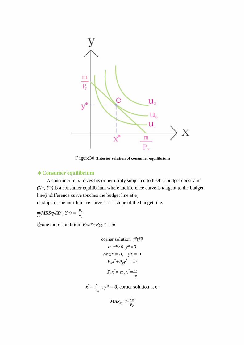
Figure30 :Interior solution of consumer equilibrium
*Consumer equilibrium A consumer maximizes his or her utility subjected to his/her budget constraint. (X*, Y*) is a consumer equilibrium where indifference curve is tangent to the budget line(indifference curve touches the budget line at e) or slope of the indifference curve at e = slope of the budget line.
or⇒MRSxy(X*, Y*) = 𝑃𝑥
𝑃𝑦
◎one more condition: Pxx*+Pyy* = m
corner solution 角解 e: x*>0, y*=0
or x* = 0, y* = 0 Pxx*+Pyy* = m
Pxx*= m, x*=𝑚𝑃𝑥
x*= 𝑚𝑃𝑥
, y* = 0, corner solution at e.
MRSxy ≥𝑃𝑥𝑃𝑦

Figure31 :Corner solution of consumer equilibrium
another corner solution:
x*= 0, y* = 𝑚𝑃𝑦
, MRSxy ≤𝑃𝑥𝑃𝑦
*In the interior solution case:
if MRSxy > 𝑃𝑥𝑃𝑦
subject change object exchange rate (主觀)個人偏好 (客觀)價錢比
x↑, y↓
Figure32 :
a→c c has more X => c is better than a. c→e
MRSxy = 𝑃𝑥𝑃𝑦
同理, MRSxy < 𝑃𝑥𝑃𝑦
=> x↓, y↑
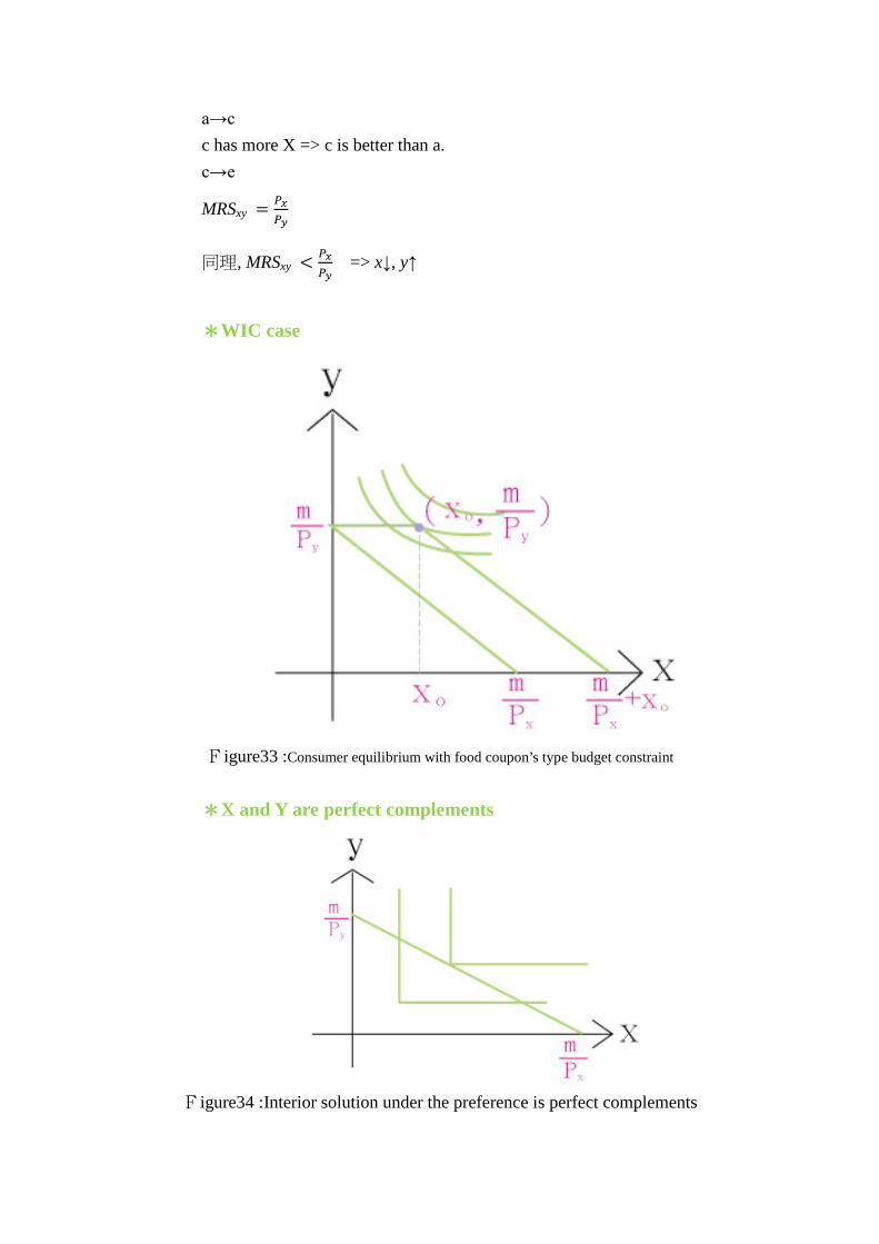
*WIC case
Figure33 :Consumer equilibrium with food coupon’s type budget constraint
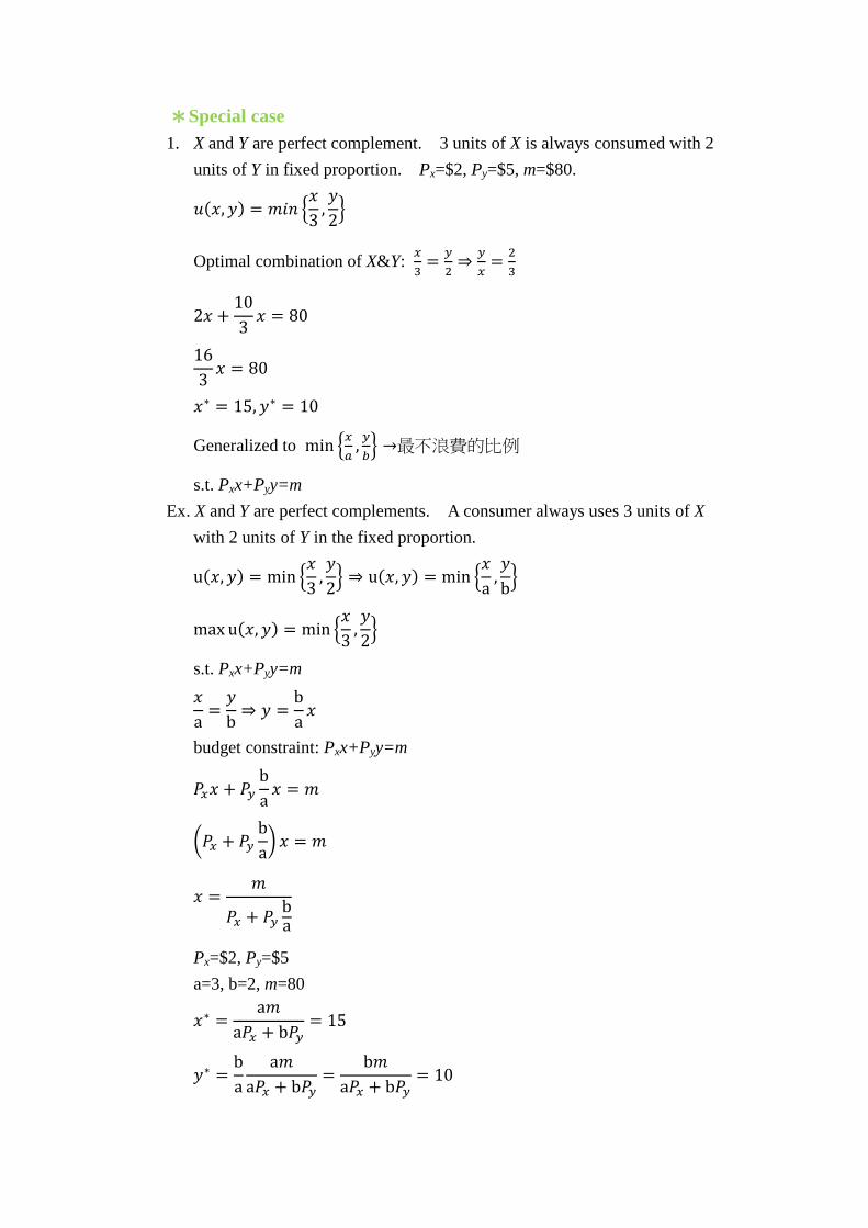
*X and Y are perfect complements
Figure34 :Interior solution under the preference is perfect complements

*To max u(x, y) s.t 𝑷𝒙 ∙ 𝒙 + 𝑷𝒚 ∙ 𝒚 = 𝒎 u(x, y) is some continuously differentiable function How to solve the consumer’s problem? General problem: max f(x. y) s.t. g(x, y) = 0
(min) ℒ(𝑥,𝑦, 𝜆) = 𝑢(𝑥,𝑦) + 𝜆(𝑚− 𝑃𝑥𝑋 − 𝑃𝑦𝑌) …Lagrange multiplier method = 𝑓(𝑥,𝑦) + 𝜆𝑔(𝑥,𝑦) constrained problem →non-constrained problem and apply FOC to the
non- constrained problem.
○1 𝜕ℒ(𝑥,𝑦,𝜆)𝜕𝑥
=𝜕�𝑢(𝑥,𝑦)+𝜆�𝑚−𝑃𝑥𝑋−𝑃𝑦𝑌��
𝜕𝑥= 𝜕𝑢(𝑥,𝑦)
𝜕𝑥− 𝜆𝑃𝑥 = 0
𝜕𝑢(𝑥,𝑦)𝜕𝑥
= 𝜆𝑃𝑥 --○1 ’
○2 𝜕ℒ(𝑥,𝑦,𝜆)𝜕𝑦
=𝜕�𝑢(𝑥,𝑦)+𝜆�𝑚−𝑃𝑥𝑋−𝑃𝑦𝑌��
𝜕𝑦= 𝜕𝑢(𝑥,𝑦)
𝜕𝑦− 𝜆𝑃𝑦 = 0
𝜕𝑢(𝑥,𝑦)𝜕𝑦
= 𝜆𝑃𝑥 --○2 ’
○3 𝜕ℒ(𝑥,𝑦,𝜆)𝜕𝜆
=𝜕�𝑢(𝑥,𝑦)+𝜆�𝑚−𝑃𝑥𝑋−𝑃𝑦𝑌��
𝜕𝜆= 𝑚− 𝑃𝑥𝑥 − 𝑃𝑦𝑦 = 0 --○3 ’
budget constraint
○1 '/○2 '=𝑀𝑢𝑥𝑀𝑢𝑦
= 𝑃𝑥𝑃𝑦
--○4
MRSxy = 𝑀𝑢𝑥𝑀𝑢𝑦
○4 MRSxy = 𝑀𝑢𝑥𝑀𝑢𝑦
=𝑃𝑥𝑃𝑦
在同樣的$1 上比較
𝑀𝑢𝑥𝑃𝑥
= 𝑀𝑢𝑦𝑃𝑦
⇒ 𝑀𝑢𝑥𝑃𝑥
= ∆𝑢(𝑥,𝑦)∆𝑥
∆𝑒𝑥𝑝𝑒𝑛𝑑𝑖𝑡𝑢𝑟𝑒∆𝑥
*Special case 1. X and Y are perfect complement. 3 units of X is always consumed with 2
units of Y in fixed proportion. Px=$2, Py=$5, m=$80.
𝑢(𝑥,𝑦) = 𝑚𝑖𝑛 �𝑥3
,𝑦2�
Optimal combination of X&Y: 𝑥3
= 𝑦2⇒ 𝑦
𝑥= 2
3
2𝑥 +103𝑥 = 80
163𝑥 = 80
𝑥∗ = 15,𝑦∗ = 10
Generalized to min �𝑥𝑎
, 𝑦𝑏� →最不浪費的比例
s.t. Pxx+Pyy=m Ex. X and Y are perfect complements. A consumer always uses 3 units of X
with 2 units of Y in the fixed proportion.
u(𝑥,𝑦) = min �𝑥3
,𝑦2� ⇒ u(𝑥,𝑦) = min �
𝑥a
,𝑦b�
max u(𝑥,𝑦) = min �𝑥3
,𝑦2�
s.t. Pxx+Pyy=m 𝑥a
=𝑦b⇒ 𝑦 =
ba𝑥
budget constraint: Pxx+Pyy=m
𝑃𝑥𝑥 + 𝑃𝑦ba𝑥 = 𝑚
�𝑃𝑥 + 𝑃𝑦ba� 𝑥 = 𝑚
𝑥 =𝑚
𝑃𝑥 + 𝑃𝑦ba
Px=$2, Py=$5 a=3, b=2, m=80
𝑥∗ =a𝑚
a𝑃𝑥 + b𝑃𝑦= 15
𝑦∗ =ba
a𝑚a𝑃𝑥 + b𝑃𝑦
=b𝑚
a𝑃𝑥 + b𝑃𝑦= 10
Ex. Cobb-Douglas utility function 𝑢(𝑥,𝑦)total utility = 𝑥α𝑦β, α, β > 0
𝑀𝑢𝑥 = ∂𝑢(𝑥,𝑦)∂𝑥
= ∂𝑥α𝑦β
∂𝑥= α𝑥α−1𝑦β > 0 no satiation point (no bliss point)
Muy = ∂u(x,y)∂y
= ∂xαyβ
∂y= βxαyβ−1 > 0
∂𝑀𝑢𝑥∂𝑥
= α(α− 1)𝑥α−2𝑦β ⇒ α < 1
𝜕𝑀𝑢𝑦𝜕𝑦
= 𝛽(𝛽 − 1)𝑥𝛼𝑦𝛽−2 ⇒ 𝛽 < 1 → 𝐷𝑖𝑚𝑖𝑛𝑖𝑠ℎ𝑖𝑛𝑔 𝑀𝑎𝑟𝑔𝑖𝑛𝑎𝑙 𝑢𝑡𝑖𝑙𝑖𝑡𝑦
𝑀𝑅𝑆𝑥𝑦 =𝑀𝑢𝑥𝑀𝑢𝑦
=𝛼𝑥𝛼−1𝑦𝛽
𝛽𝑥𝛼𝑦𝛽−1=𝛼𝛽𝑦𝑥→ �𝑥越大,𝑦越小� ⇒
𝑑𝑀𝑅𝑆𝑥𝑦𝑑𝑥
< 0
For any α, β>0 and for all x and y 𝑑𝑀𝑅𝑆𝑥𝑦𝑑𝑥
< 0
i.e. MRSxy is diminishing (with x) i.e. indifference curve is always convex
In equilibrium, 𝑀𝑅𝑆𝑥𝑦 = 𝑃𝑥𝑃𝑦
𝛼𝛽𝑦𝑥
=𝑃𝑥𝑃𝑦
𝑃𝑦𝑦(expenditure on Y) =𝛽 𝛼𝑃𝑥𝑥(expenditure on 𝑋)
𝑃𝑥𝑥 + 𝑃𝑦𝑦 = 𝑚
𝑃𝑥𝑥 +𝛽 𝛼𝑃𝑥𝑥 = 𝑚
𝛼 + 𝛽 𝛼
𝑃𝑥𝑥 = 𝑚⟹ 𝑒𝑥(expenditure of x) = 𝑃𝑥𝑥 =𝛼
𝛼 + 𝛽 𝑚(short of 𝑒𝑥)
𝑒𝑦(expenditure of y) = 𝑃𝑦𝑦 =𝛽
𝛼 + 𝛽 𝑚(short of 𝑒𝑦)
𝑥∗ =𝛼
𝛼 + 𝛽𝑚𝑃𝑥
𝑦∗ =𝛽
𝛼 + 𝛽𝑚𝑃𝑦


![[PPT]Consumer Behavior and Marketing Strategy - Lars … to CB.ppt · Web viewIntro to Consumer Behavior Consumer behavior--what is it? Applications Consumer Behavior and Strategy](https://static.fdocuments.in/doc/165x107/5af357b67f8b9a74448b60fb/pptconsumer-behavior-and-marketing-strategy-lars-to-cbpptweb-viewintro.jpg)