


Languages
Pages
Legal


Categorical Datatesting associations between categorical variables
Categorical Data
Today’s goal: Teach you about methods to test associations between two or more categorical variables
Outline:
- Two variables: Chi-square test
- More than two variables: loglinear analysis (bonus)

Chi-square testtesting associations between two categorical variables

Chi-square testIs there a relation between reward and whether a cat can learn to dance?
Food Affection Total
Dance 28 48 76
No dance 10 114 124
Total 38 162 200

Chi-square testWhat values would we expect if there was no relation?
row total * column total / grand total
Food Affection Total
Dance 14.44 61.56 76
No dance 23.56 100.44 124
Total 38 162 200
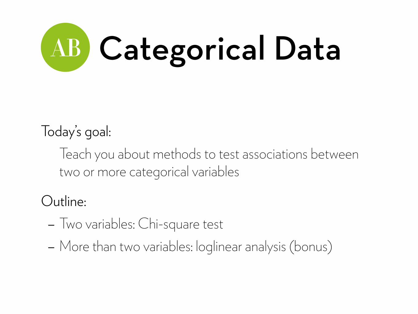
Chi-square testWhat is the deviation from this model?
(observed – model)2
Food Affection TotalDance 14.44 61.56 76
No dance 23.56 100.44 124Total 38 162 200
Food Affection TotalDance 28 48 76
No dance 10 114 124
Total 38 162 200
Food Affection
Dance 183.9 –183.9
No dance –183.9 183.9
–( )2
=

Chi-square testCan we standardize these deviations?
Σ((observed – model)2 / model)Food Affection Total
Dance 14.44 61.56 76
No dance 23.56 100.44 124Total 38 162 200
Food Affection
Dance 183.9 –183.9
No dance –183.9 183.9/=
Food Affection
Dance 12.73 7.80
No dance 2.99 1.83= 25.35

Chi-square test
Σ((observed – model)2 / model) is a χ2 statistic It has (r–1)(c–1) degrees of freedom
Chi-square works well for large samples For smaller samples, make Yates’s correction: Σ((|observed – model|–0.5)2 / model) For even smaller samples (expected count < 5 for more than 20% of the cells), use Fisher’s exact test

Assumptions
Independence
Expected frequencies > 5 for at least 20% of the table All expected frequencies should be > 1 Use Fisher’s exact test if not

Chi-square in RDataset “cats.dat”
Effect of reward on cats’ ability to learn how to dance
Variables: Training: whether the cat got food or affection as reward Dance: whether the cat learned how to dance (Yes/No)
Or, use a table: catTable <- cbind(“Dance" = c("Food"=28, "Affection"= 48), "No dance" = c("Food" = 10, "Affection" = 114))

Chi-square in RPlotting from the table:
mosaicplot(catTable,shade=T)
Run the chi-square test (in package “gmodels”): CrossTable(cats$Training, cats$Dance, expected=T, fisher=T, sresid=T,format=“SPSS”)
Or from the table: CrossTable(catTable, expected=T, fisher=T, sresid=T,format=“SPSS”)
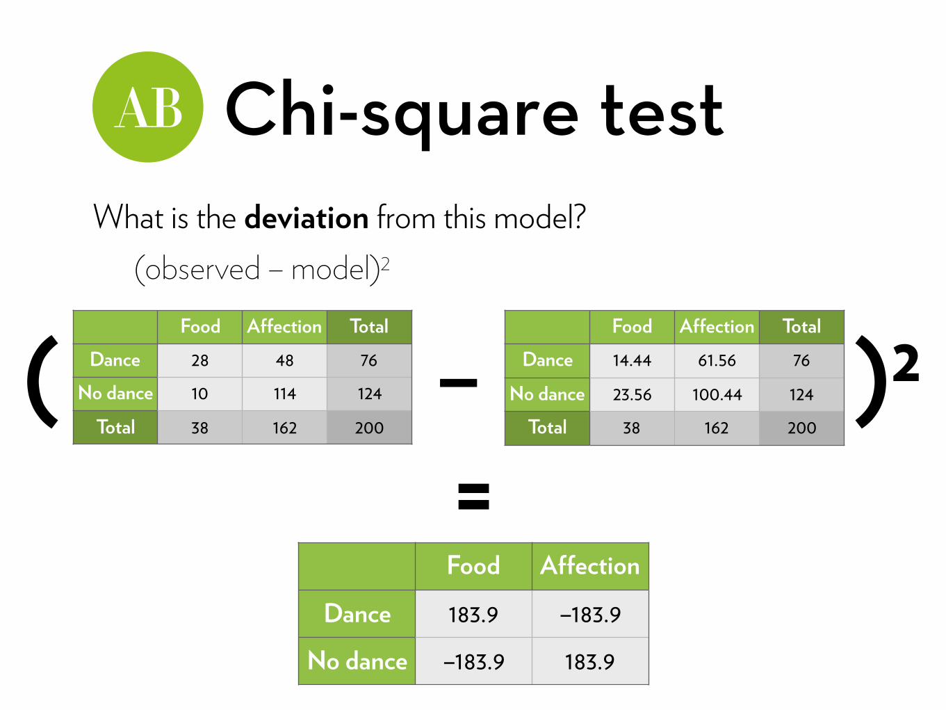
Chi-square in RInterpretation of table:
Observed count in this cell and predicted count in this cell Standardized deviance in this cell (adds up to Chi-square) Percentage in this row (70.4% of cats who got affection did not learn how to dance, 29.6% did) Percentage in this column (91.9% of cats who did not learn how to dance got affection, 8.1% got food) Overall percentage Standardized residual (see later)

Chi-square in R
Interpretation of test results: Chi-square test: apparently there is a strong association, because χ2(1) = 25.36 has a p < .0001 Chi-square with Yates’ correction is very similar (23.52) Fisher’s exact test also finds significance (the remaining two rows are one-sided exact tests) Minimum frequency is 14.44, which is larger than the required 5

Finding the effectLike ANOVA, when there are more than 2 conditions/levels, the chi-square finds out if there is an effect, not where the effect is
Like ANOVA, we can break down the significant test into smaller portions
For the chi-square test, we use standardized residuals:
z = (observed – model)/√(model)
This is the “unsquared” version of the deviation in each cell And guess what… It’s a z-score!

Finding the effectWhen food was used as a reward:
…significantly more cats than expected danced (z = 3.57) …and significantly fewer cats than expected didn’t dance (z = –2.79)
When affection was used as a reward: No significant differences from what we expected
The significance is mainly driven by the food condition
(This stuff gets more interesting in larger tables)

Effect size
A chi-square effect in a 2x2 table can be expressed as an odds ratio
Odds of dancing after food = 28/10 = 2.8 Odds of dancing after affection = 48/114 = 0.421 Odds ratio: 2.8/0.421 = 6.65
In R, Fisher’s exact test gives you a (better) odds ratio, plus a confidence interval
If this interval doesn’t cross 1, the odds ratio is significant!

Reporting
There was a significant association between the type of training and whether a cat would learn how to dance χ2(1) = 25.36, p < .001. The odds of cats dancing were 6.58 times higher if they were trained with food than if they were trained with affection (95% CI: [2.84, 16.43]).

As a logistic regSince Dance has 2 categories run this as a logistic regression:
c1 <- glm(Dance ~ Training, data=cats, family=binomial)
Odds ratio and CI are similar: exp(c1$coefficients) exp(confint(c1))
Chi-square is similar as well: anova(c1) 1-pchisq(c1$null.deviance-c1$deviance, 1)

Expand to 3 varsDataset “CatsandDogs.dat” -> rename to “catdog”
Effect of reward on cats’ and dogs’ ability to dance
Variables: Animal: whether this was a cat or a dog Training: whether the animal got food or affection Dance: whether the animal learned how to dance
Plotting: mosaicplot(table(catdog), shade=T)
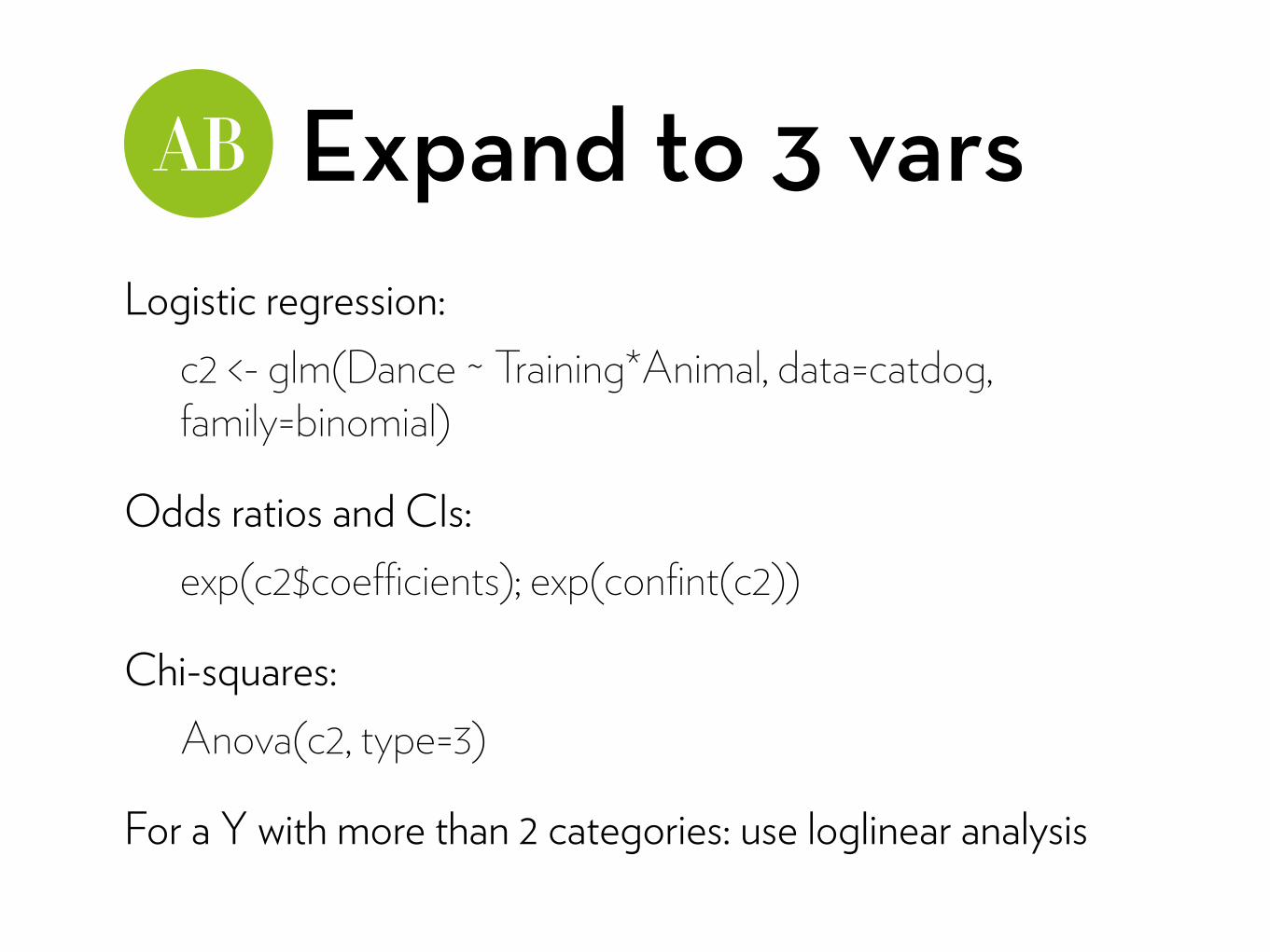
Expand to 3 varsLogistic regression:
c2 <- glm(Dance ~ Training*Animal, data=catdog, family=binomial)
Odds ratios and CIs: exp(c2$coefficients); exp(confint(c2))
Chi-squares: Anova(c2, type=3)
For a Y with more than 2 categories: use loglinear analysis

3x4 chi-square
Dataset “favorite.csv” Relationship between favorite party game and party snack
Variables: Game: favorite party game Snack: favorite party snack
Plotting: mosaicplot(table(favorite), shade=T)

Chi-square in R
Run the chi-square test: CrossTable(favorite$Game, favorite$Food, expected=T, fisher=T, sresid=T,format=“SPSS”)
Interpretation of test results:
Chi-square test: χ2(6) = 14.51, p = .024 Fisher’s exact test also finds significance Minimum frequency is 6, which is larger than the required 5

Finding the effect
Analyze residuals: Poker players are less likely to prefer chips (z = -1.981) Poker players are more likely to prefer cookies (z = 2.145)
We can calculate an odds ratio, but only in a 2x2 table. So let’s compare poker players vs. others, and cookies vs. chips:
Odds of cookies for poker players = 12/3 = 4.00 Odds of cookies for others = 18/38 = 0.474 Odds ratio: 4.00/0.474 = 8.44

There was a significant association between the favorite party game (Monopoly, poker, Trivial Pursuit, or Wii Bowling) and favorite party snack (chips and dip, cookies, or pizza rolls) χ2(6) = 14.51, p = .024. Upon analyzing the effect, we found that the odds of liking cookies rather than chips were 8.44 times higher for poker players than for others.
Reporting

Loglinear analysistesting associations between several categorical variables
(this will not be on the test)

Loglinear analysisWe can see a chi-square test as a Poisson regression with 4 data points:
Training = Affection Dance Interaction Frequency
0 0 0 100 1 0 281 0 0 1141 1 1 48
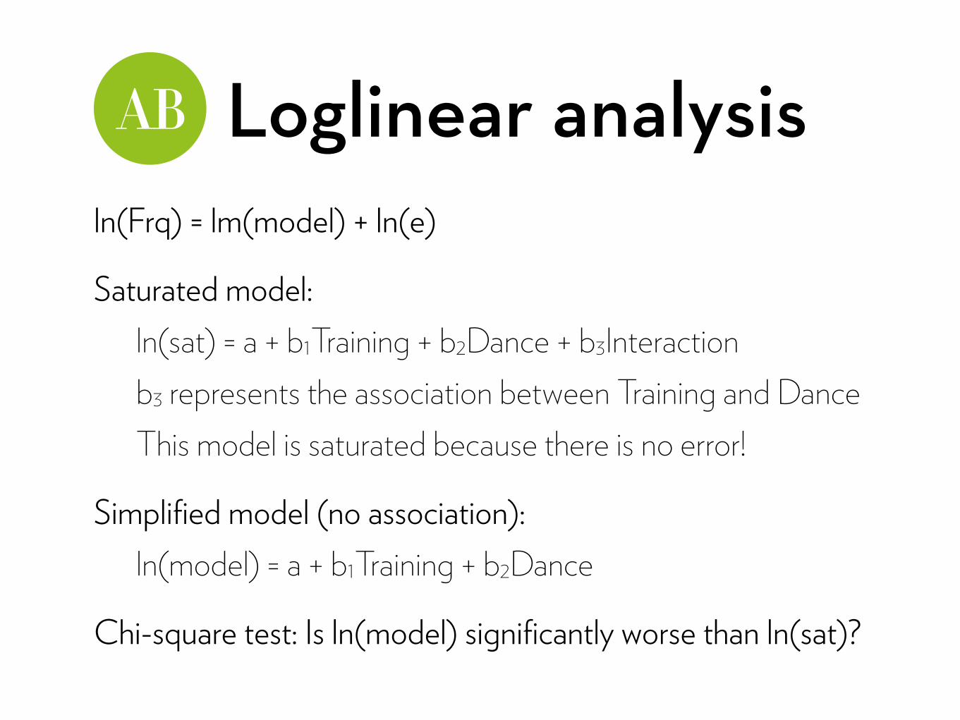
Loglinear analysisln(Frq) = lm(model) + ln(e)
Saturated model: ln(sat) = a + b1Training + b2Dance + b3Interaction b3 represents the association between Training and Dance This model is saturated because there is no error!
Simplified model (no association): ln(model) = a + b1Training + b2Dance
Chi-square test: Is ln(model) significantly worse than ln(sat)?

Loglinear analysisExtension: If we have three variables, our saturated model becomes:
ln(model) = a + b1A + b2B + b3C + b4AB + b5AC + b6BC + b7ABC
Backward elimination: What if we remove ABC? Much worse? Then stop! If not: What if we remove AB, AC, or BC? Much worse? Stop! If not: A, B, and C are independent
We use the likelihood ratio (Lχ2change = L χ2current – Lχ2previous)
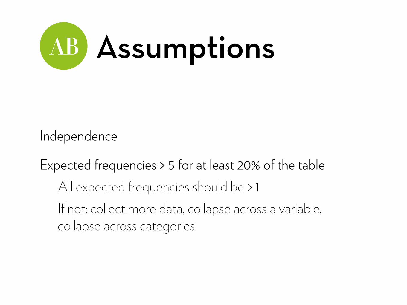
Assumptions
Independence
Expected frequencies > 5 for at least 20% of the table All expected frequencies should be > 1 If not: collect more data, collapse across a variable, collapse across categories
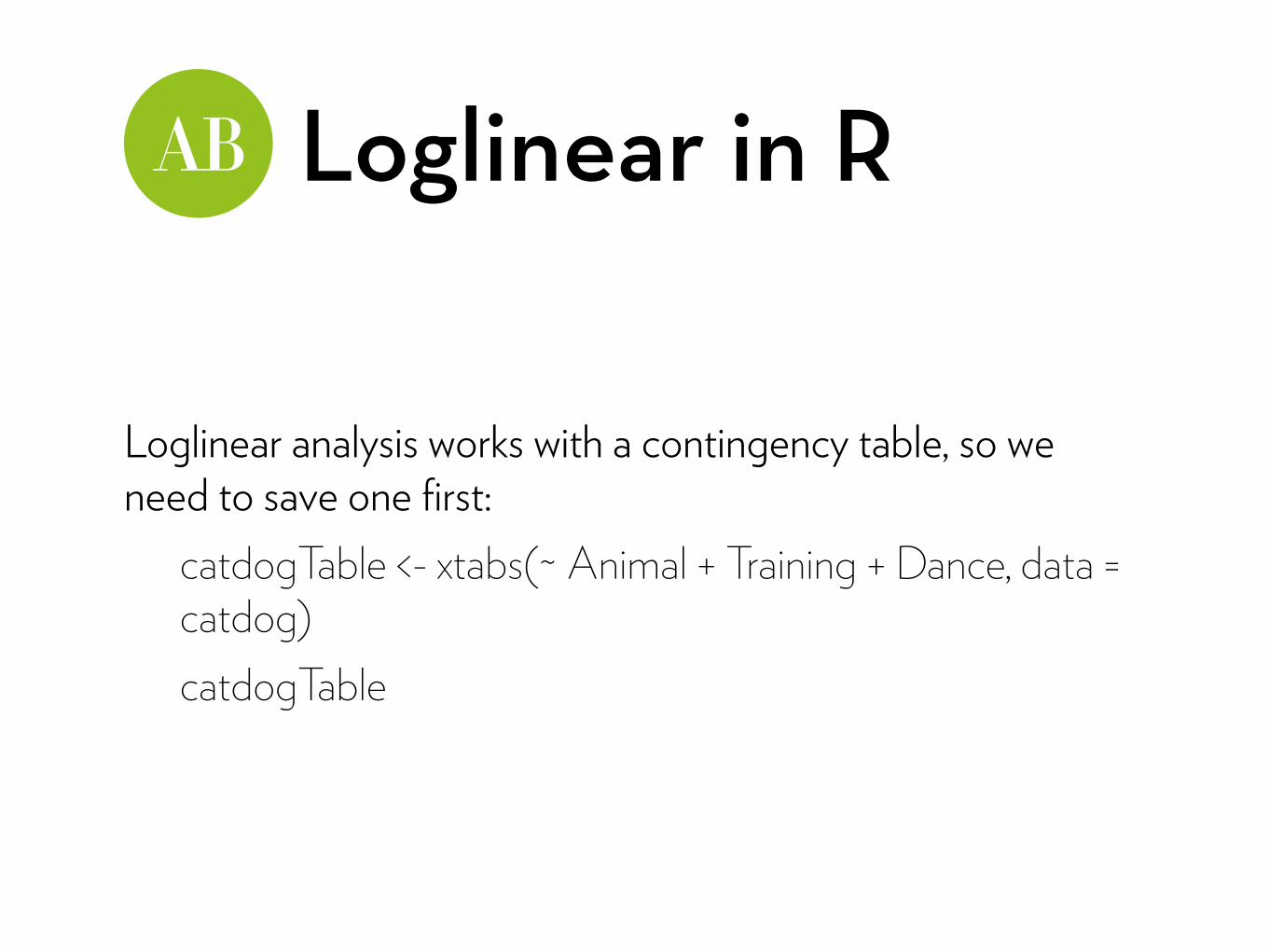
Loglinear in R
Loglinear analysis works with a contingency table, so we need to save one first:
catdogTable <- xtabs(~ Animal + Training + Dance, data = catdog) catdogTable

Run analysesCreate a saturated model:
saturated <- loglm(~ Animal*Training*Dance, data = catdogTable) summary(saturated) — bottom part shows perfect fit
Remove the three-way interaction: threeway <- update(saturated, .~. - Animal:Training:Dance) summary(threeway) — Fit is not as good…
Compare the models: anova(saturated, threeway)

Let’s continue…Create three models removing each two-way interaction:
trainingDance <- update(threeWay, .~. - Training:Dance) animalDance <- update(threeWay, .~. - Animal:Dance) animalTraining <- update(threeWay, .~. - Animal:Training)
Get the ANOVAs: anova(threeway, trainingDance) — significant! anova(threeway, animalDance) — significant! anova(threeway, animalTraining) — significant!

InterpretationOK, so there’s a 3-way effect…
How do we interpret it?
Let’s plot it! mosaicplot(catdogTable, shade=T)
Interpretation: Both cats and dogs are more likely to dance for food Dogs are more likely to dance for affection, too Cats are less likely to dance for affection

Follow up
You can now do separate chi-squares in separate groups
You already did a chi-square for cats: CrossTable(cats$Training, cats$Dance, expected=T, fisher=T, sresid=T,format=“SPSS”)
For dogs, first create justDogs <- subset(catdog, Animal==“Dog”):
CrossTable(justDogs$Training, justDogs$Dance, expected=T, fisher=T, sresid=T,format=“SPSS”)

Effect size
Get the odds ratio for cats and dogs: Odds ratio for cats: 6.65 Odds ratio for dogs: 0.35 (see Fisher test)
Interpretation Dogs are 2.86 times more likely to dance for affection than for food (1/0.35 = 2.90) Cats are 6.65 times more likely to dance for food than for affection
Reporting
The three-way loglinear analysis demonstrated that the three-way interaction of Animal, Training and Dance was significant, χ2(1) = 20.31, p < .001. We subsequently performed separate analyses for cats and dogs.
For cats, there was a significant association between the type of training and whether they would learn how to dance χ2(1) = 25.36, p < .001. The odds of cats dancing were 6.58 times higher if they were trained with food than if they were trained with affection.

Reporting
For dogs, there was also a significant association between the type of training and whether they would learn how to dance χ2(1) = 3.93, p < .05. However, in contrasts to cats, the odds of dogs dancing were 2.90 times lower if they were trained with food than if they were trained with affection.

“It is the mark of a truly intelligent person to be moved by statistics.”
George Bernard Shaw
Top Related