Digital Object Identifier (DOI):10.1007/s00285-006-0376-4

J. Math. Biol. (2006) Mathematical Biology

Alan Grafen

A theory of Fisher’s reproductive value

Received: 9 February 2005 / Revised version: 19 December 2005 /Published online: 24 April 2006 – c© Springer-Verlag 2006

Abstract. The formal Darwinism project aims to provide a mathematically rigorous basisfor optimisation thinking in relation to natural selection. This paper deals with the situation inwhich individuals in a population belong to classes, such as sexes, or size and/or age classes.Fisher introduced the concept of reproductive value into biology to help analyse evolutionaryprocesses of populations divided into classes. Here a rigorously defined and very generalstructure justifies, and shows the unity of concept behind, Fisher’s uses of reproductive valueas measuring the significance for evolutionary processes of (i) an individual and (ii) a class;(iii) recursively, as calculable for a parent as a sum of its shares in the reproductive values ofits offspring; and (iv) as an evolutionary maximand under natural selection. The maximand isthe same for all parental classes, and is a weighted sum of offspring numbers, which impliesthat a tradeoff in one aspect of the phenotype can legitimately be studied separately fromother aspects. The Price equation, measure theory, Markov theory and positive operatorscontribute to the framework, which is then applied to a number of examples, including anew and fully rigorous version of Fisher’s sex ratio argument. Classes may be discrete (e.g.sex), continuous (e.g. weight at fledging) or multidimensional with discrete and continuouscomponents (e.g. sex and weight at fledging and adult tarsus length).

Contents

1. Introduction . . . . . . . . . . . . . . . . . . . . . . . . . . . . . . . . . . . . .2. Overviews of the paper . . . . . . . . . . . . . . . . . . . . . . . . . . . . . . .

2.1. An overview in words . . . . . . . . . . . . . . . . . . . . . . . . . . . .2.2. A mathematical overview . . . . . . . . . . . . . . . . . . . . . . . . . .

3. Price for classes . . . . . . . . . . . . . . . . . . . . . . . . . . . . . . . . . . .3.1. Link to Markov theory . . . . . . . . . . . . . . . . . . . . . . . . . . . .3.2. The Price equation with classes . . . . . . . . . . . . . . . . . . . . . . .

4. Existence and uniqueness of reproductive value . . . . . . . . . . . . . . . . . .4.1. The forwards process . . . . . . . . . . . . . . . . . . . . . . . . . . . . .4.2. Links between the forward and backwards processes . . . . . . . . . . . .4.3. Useful theorems on existence and uniqueness . . . . . . . . . . . . . . . .4.4. Uniqueness . . . . . . . . . . . . . . . . . . . . . . . . . . . . . . . . . .4.5. Examples . . . . . . . . . . . . . . . . . . . . . . . . . . . . . . . . . . .

5. Interpretation of reproductive value . . . . . . . . . . . . . . . . . . . . . . . . .6. Equilibrium under natural selection with classes . . . . . . . . . . . . . . . . . .

6.1. Clonal growth . . . . . . . . . . . . . . . . . . . . . . . . . . . . . . . .6.2. Stubblefield’s ‘tracer-allele’ method . . . . . . . . . . . . . . . . . . . . .6.3. Comparison of the concepts . . . . . . . . . . . . . . . . . . . . . . . . .

A. Grafen: St John’s College, Oxford OX1 3JP, United Kingdom.e-mail: alan.grafen@sjc.ox.ac.uk

Key words or phrases: Reproductive Value – R.A. Fisher – Class-structured population –Natural Selection – Formal Darwinism – Optimisation

A. Grafen

7. Fisher’s four uses of reproductive value . . . . . . . . . . . . . . . . . . . . . .8. Examples . . . . . . . . . . . . . . . . . . . . . . . . . . . . . . . . . . . . . .

8.1. A sex ratio model . . . . . . . . . . . . . . . . . . . . . . . . . . . . . . .8.2. Rank order for resources, and a non-compact X . . . . . . . . . . . . . . .8.3. A geographical example . . . . . . . . . . . . . . . . . . . . . . . . . . .

9. Comparison with Taylor . . . . . . . . . . . . . . . . . . . . . . . . . . . . . . .10. Conclusions . . . . . . . . . . . . . . . . . . . . . . . . . . . . . . . . . . . . .

1. Introduction

The concept of reproductive value was introduced into biology by Fisher (1930),and is now used in the study of age-structured populations (Charlesworth, 1994)and by ecologists in the study of populations with age and other kinds of structuretoo (Caswell, 1989; Easterling et al. , 2000). Reproductive value is a quantitativemeasure for subsets of a population, including individuals, that indicates their rel-ative importance in evolutionary processes. In fact this paper will show that thequantitative measure plays four roles. Some are more familiar to biologists, othersto population geneticists, and the analysis will show that the roles are all tightlyinterlinked.

First, each individual in the population has a numerical value attached to it thatis its reproductive value, and when taking an average gene frequency, the repro-ductive values should be used as individual weights. The sense of ‘should’ is thatif we do so, average gene frequency will behave nicely. For example, if there aretwo alleles at a locus and they have identical effects, their average gene frequencieswon’t change. Thus an individual’s reproductive value measures its contribution tothe gene pool of future generations.

Second, subsets of the population, such as males and females, or large and small,have reproductive values, and when calculating an average gene frequency over thewhole population, they should be used as weights: note that the reproductive valueof a subset, apart from some possible re-scaling for convenience, does equal theaggregate of the reproductive values of the individuals in the subset. One interesthere is that sometimes it is possible to calculate the reproductive value of a wholesubset, knowing nothing about the individuals, as in Fisher’s famous sex ratio argu-ment showing that in diploids all males together have the same reproductive valueas all females together. In this sense, we can think of the reproductive value of allmales as the fraction of genes in a future generation whose ancestor is present ina male in this generation. Hence the reproductive value of a subset measures itsgenetic contribution to future generations.

Third, an offspring has a reproductive value, and each parent has a share in it,depending on the fraction of the offspring’s genes it contributed; the reproductivevalue of a parent equals the sum of its shares in the reproductive value of its off-spring. This reveals reproductive value as a generalisation of counting a parent’soffspring, and it also becomes possible to ask what the parent’s reproductive valuewould have been if different strategies had been followed.

Finally, there is a role as maximand. In simple models without classes, a genefrequency increases if the gene confers higher number of offspring on its bear-ers. This can be translated into more formal links showing that natural selection

A theory of Fisher’s reproductive value

tends to lead to maximisation of number of offspring or, more precisely, of ex-pected relative number of offspring (Grafen, 2002). By using reproductive valueas weights, we will obtain a generalisation to the case with classes: average genefrequency (when weighted with reproductive value) increases if the gene confers ahigher reproductive value on its bearers. This gives us a maximisation principle forreproductive value, though it will not made formally explicit until the examples inSection 8.

It is worth noting that there has been confusion in discussing ‘evolutionarymaximands’ between dynamic concepts such as Lyapunov functions and poten-tial functions on the one hand, and on the other, the idea that individual organ-isms will be selected to act as if maximising some function. It is the second thatwill be discussed here, and the reader is referred to Grafen (1999) for furtherdiscussion.

There are many significances in establishing such a reproductive value in a widerange of models. At the most obvious level, it helps to tame complex situations withclasses, and provides results parallel to the simple model with only one class. Moreambitiously, it brings precision to the biologist’s frequent use of ‘reproductive value’as a more precise version of ‘fitness’. It leads mathematical population geneticists tosee that the first three properties, with which they are familiar in particular contexts,hold very generally and are linked to maximisation. It extends the range of modelsin which an optimisation principle has already been demonstrated (Grafen, 2002,2006) to include models in which classes exist. Population geneticists have since aninfluential paper of Moran (1964) rejected the concept of an optimisation principlein population genetics, so it is relevant that this paper establishes the nature andexistence of reproductive value in a very general setting with full mathematicalrigour. Finally, the paper shows that the original informal use of reproductive value(Fisher, 1930) can be fully justified in that very general setting.

When, from a biological point of view, does the concept of reproductive valueof classes become important in applications? Examples include sex ratio, whereoffspring may be male or female; parental care, in which offspring receiving morecare must somehow count more than those who receive less; and geography, wherethe location of an offspring may matter. A technical example is age-structured pop-ulations, which can be handled within a non-overlapping generations frameworkby treating survival from year t to year t + 1 as the production by an age t adultof an asexual age t + 1 offspring. It is also possible, for example, to define classesin the population with respect to one genetic locus while studying changes in genefrequencies at another.

The current paper builds on the work of Taylor (1990, 1996), who considereda finite set of classes. Here the analysis is linked explicitly to Fisher’s reproductivevalue arguments, showing that Fisher used a very general framework we are onlynow coming to understand. By allowing the set of classes to be finite or infinite, andto include single and multi-dimensional continuous variables, the range is extendedof examples to which reproductive value can be applied. Finally, the treatment herecontributes to the formal Darwinism project (Grafen, 1999, 2000, 2002, 2006),which aims to represent in as general a way as possible Darwin’s arguments aboutthe operation of natural selection. The arbitrariness of the set of classes, and the

A. Grafen

fact that the argument handles them all in a single formulation rather than provid-ing separate cases for different kinds of sets, contributes significantly to the claimthat the project captures Darwinian natural selection in general. It is also importantfor the project that some of the results obtained here apply under a more generalgenetics than Taylor’s.

The formalism developed in this paper therefore allows new kinds of examplesto be studied using reproductive value methods. One so far hypothetical examplewould be of parental care in birds, where the type of care provided by parents affectsthe fledging weight and tarsus length of sons and daughters. The reproductive valueweights would provide a maximand that would allow a parent to choose which com-bination of fledging weight and tarsus length was best for sons, and which was bestfor daughters. The optimal balances could be different for parents from differentclasses. Suppose tarsus length is used in mate choice. The weights would thenincorporate sex-ratio selection and sexual selection, as well as any differences insimple viability, to provide a single quantity with important properties under naturalselection that biologists might well be tempted to call ‘fitness’.

There are important restrictions on the analysis. To incorporate classes in theabsence of uncertainty, it has proved necessary to assume the population is infi-nite. We also assume discrete, non-overlapping generations and that an individualremains in the same class throughout its life, which excludes important areas ofreproductive value. For example, reproductive value has been used to study sex ratiounder partial bivoltinism (Grafen, 1986), and to study cases in which individualscan affect their own class from one year to the next (Grafen, 1987). Thus, we dealhere only with classes that are chosen by parents, and that offspring bear for theirlifetime. Defining reproductive value outside these assumptions is an importanttask.

There are further restrictions. Individuals are assumed to affect only their ownnumber of offspring, so that social behaviour as introduced by Hamilton (1964) isexcluded. Grafen (2006) incorporates social behaviour into the formal Darwinismproject, but not in a way that combines it with classes and reproductive value. Fre-quency-dependent selection is not explicitly modelled, and most forms of it wouldrequire a more elaborate model, and a more complex analysis, than that presentedhere. However, sex ratio selection is included.

Some sections are designed to be readable by non-mathematical biologists,who are prepared to endure some necessary limited notation. Section 2 providesan overview of the rest of the paper without mathematical technicalities, and thenan account of the mathematical manoeuvres employed in each section. Section 5gives a reasonably non-technical explanation of how the concept of reproductivevalue links to the formal idea of invariant measures, and of the biological signifi-cance of non-uniqueness. Section 7 discusses Fisher’s uses of reproductive value,and how the analysis of the current paper justifies the implicit structure, while Sec-tion 10 briefly concludes. The other sections are quite technical, and require somemathematical ambition.

A theory of Fisher’s reproductive value

2. Overviews of the paper

A marked feature of this paper is that the mathematics presented is very formal,and daunting even to the author. This overview section first presents an outline ofthe paper, section by section, without technicalities. The following subsection dis-cusses the mathematical concepts used, explains the need for the formalities, andjustifies the absence of a simple pedagogical example.

2.1. An overview in words

The main purpose is to provide a mathematically rigorous exposition of how optimi-sation ideas can be applied to the operation of natural selection when the populationis divided into classes. There are a number of steps. First, Section 3 derives the PriceEquation in the presence of classes, and then focusses on how genes flow from classto class across the generations. The pattern of flow is used to define the reproductivevalues of the classes. Section 4 considers whether a pattern of flow always definesreproductive values, and if so, whether it defines them uniquely. It also establishesthe central property that reproductive value allows an evaluation in one generationof the asymptotic number of descendants. This is a highly technical section, butthe biological interpretation of these issues is set out as intelligibly as possiblein Section 5. Although no fully general result can be established, it is likely thatreproductive value can be defined in a wide range of biologically useful situations.

The target of selection, which becomes the maximand individuals are selectedto act as if maximising, has two important features. It is the same for parents in allclasses. It is a sum of contributions to offspring, weighted by offspring class, andso tradeoffs in one aspect of phenotype can legitimately be separated from otheraspects.

Section 6 studies equilibrium concepts of gene dynamics, an essential part ofstudying the operation of natural selection. The ‘tracer-allele’ approach (Seger &Stubblefield, 2002) is adopted, but there is an ambivalence of concepts that requiressome discussion. The first main result is one of the defining properties of repro-ductive value identified by Fisher (1930) and later authors, that it allows a way tomeasure natural selection that has the following desirable property: no matter howtwo alleles are distributed across classes, there is no net selection if their phenotypiceffects are identical. If we use any other weights to aggregate the gene frequencychanges across classes, then two alleles with identical effects can undergo selectivechange relative to each other. The second result shows how reproductive value pro-vides a maximand for an optimisation approach to the outcome of natural selection.

Section 7 reviews the uses of ‘reproductive value’ by Fisher (1930), and showshow they can be formally justified in detail. This section therefore shows that theelaborate mathematical machinery constructed in earlier sections has considerablebiological significance. In particular, it shows that reproductive value provides amaximand of natural selection, in the sense that natural selection tends to lead toindividuals who act as if maximising their reproductive value.

The mathematical machinery of earlier sections is put to use in Section 8, inthree examples that are only a sample of the range of possible applications, but

A. Grafen

which do show how the very abstract formulations can be brought to bear on par-ticular cases. A fully rigorous version of Fisher’s sex ratio argument is given, alongwith a development only possible using the results of this paper. Then there is anexample of parental care where the classes belong to an interval on the real line,and a geographical example where class represents location. These examples areall small-scale, as a substantial example would require a paper of its own.

In Section 9 the links with the work of Taylor (1990, 1996) are discussed. Thereis a small concluding section.

2.2. A mathematical overview

The considerable mathematical machinery is all needed for a purpose. Here, someof the choices are explained. Section 3 introduces a model beginning with the setof individuals I , which is assumed infinite. The set of classes X is treated in a verygeneral way: technically it is assumed to be compact Hausdorff. This means X is acompact topological space, and for every ordered pair of distinct points there is anopen set that contains the first of the pair but not the second. X is thus permittedto be any compact subset of R

n, which seems general enough for many biologi-cal purposes. Infinite-dimensional phenotype spaces have been used (e.g. Grafen,1990), and so the capacity to handle infinite-dimensional spaces of classes may alsobe useful – though note that the space must be compact. Both I and X are treatedas measure spaces, and the distribution of offspring classes produced by each indi-vidual is treated as a measure over X. The frequency of alleles is studied using thecovariance selection mathematics of Price (1970), but not the later extensions ofPrice (1972). The machinery of measure theory is required because of the desireto present a single argument covering all cases: the simpler notation for finite X

or for densities on the real line would not have covered the other of those cases.The population I is assumed infinite to allow exact results to be obtained. A finiteI over an infinite X could only adopt an atomic distribution; and finite I wouldnot ensure that fairness of meiosis on average guaranteed fairness of meiosis inoutcome. Another important reason for using measure theory is that the set of den-sities does not form a complete space and existence results would fail: a sequence ofdensities can converge to a distribution with atoms. It is quite likely in applicationsthat equilibrium distributions would have atoms, and also that optimal responseswould be atomic distributions.

Once it is decided to use measure theory, it becomes difficult to follow thevery reasonable suggestion of referees of an earlier version, to provide a simplemathematical example to explain the concepts. The added notation required, andthe different kind of notation required for discrete X or to consider densities on thereal line, would render unwieldy the already considerable mathematical notation ofthe paper. Many of the concepts are developed for discrete X, and explained verywell, by Taylor (1990, 1996), who could be read alongside.

The use of Radon-Nikodym derivatives should be mentioned. If we have a mea-sure over a space, and an L1 function on that space, it is a standard result that we canproduce a new measure by integrating the function with respect to the original mea-sure. The inverse process, of finding the L1 function that will convert one measure

A theory of Fisher’s reproductive value

into another, is Radon-Nikodym differentiation, and it will be needed in variouscontexts because I and X are measure spaces.

Another formalism introduced in Section 3 is a Markov process over the statespace X. The Price Equation takes us from parents in one generation to offspring inthe next. Markov theory is used to extrapolate the effects on gene frequencies thatwould follow if the class-to-class transition pattern from one generation to the nextwere to be repeated indefinitely. This hypothetical repetition allows reproductivevalue to be defined in terms of an invariant measure of the Markov process.

The questions of existence and uniqueness of that invariant measure are thesubject of Section 4. The general applicability of the concept of reproductive valuedepends on how widely an invariant measure exists for the Markov process of thepreceding section. Theorems are drawn from the literature and are applied in gen-eral, and in a series of examples that also shows how the mechanics of the Markovprocess work. Although an example is found in which none of the general resultsguarantee existence, even there an invariant measure is exhibited: the general senseis that reproductive value exists in most biologically plausible cases with a stabledistribution of the population over classes. The section actually begins by defin-ing a ‘forwards process’, which follows gene frequencies forwards in time: thiscorresponds to the ‘backwards process’ represented by the Markov process, whichfollows reproductive value backwards in time. The forwards process is useful instudying the backwards process, and also in considering equilibrium concepts laterin the paper. The invariant measure is by no means always unique, and the natureof sets of invariant measures is discussed along with their biological significancein Section 5.

Section 6 looks at equilibrium under natural selection, finding a very naturalresult linking equilibrium in the presence of classes to conditional expectations.Optimisation results can be obtained very generally in Darwinian models (Grafen,2002, 2006). One of the main purposes of the project is to set the strategic approachon an equal footing with the population genetics approach in terms of mathemati-cal rigour, so that choices between them can be made on the grounds of biologicalutility. It is therefore significant, and requires discussion in Section 6, that whenclasses are added, there is an ambivalence of equilibrium concept even within thestrategic approach.

Explicit optimisation programs are employed in the examples in Section 8,where it is easier to do because the need for complete consistency and generalityno longer holds. In previous papers (Grafen 2002, 2006) explicit optimisation wasemployed in general, as there was substantial work to do at that level, for exampleincorporating uncertainty into the maximand of natural selection. In the currentpaper, the additional notational requirements would not have been worthwhile.

Section 9 includes the correspondents in this paper to the left and right eigen-vector results for the forwards and backwards processes of Taylor (1990, 1996).

3. Price for classes

This section aims to develop the covariance selection mathematics of Price (1970)as applied to a population whose members and whose members’ offspring each

A. Grafen

belong to a class. The approach chosen employs measure theory rather than thealternative of generalised functions (Kanwal, 1983), for compatibility with previ-ous work extending the Price equation to uncertainty (Grafen, 2002). This holdsout the prospect of a combined model developing a rigorous treatment of the casecombining classes and uncertainty.

The Price equation assumes a census point in the parent and offspring genera-tions. All individuals at the first census point are parents, and each leaves a certainnumber of successful gametes, that is, gametes which contribute to an offspringpresent at the second census point. We will assume in the words we use that thecontribution of a parent to an offspring is exactly one gamete, which holds formost situations in diploidy, haploidy and haplo-diploidy. The formalism actuallyextends more widely, if we understand counting offspring to be counting successfulgametes. This extension matters because the framework does apply to a model ofmixed sexual and asexual reproduction in diploids, for example, including whereparental survival is formally represented as asexual reproduction; and to the arbi-trary ploidy models of Grafen (1986), as in Section 8.1. However, it would be toocumbersome to have to read ‘successful gamete’ in all the necessary places. Weimmediately assume, though it is not needed until Section 4.1, that all individualsin the same class share the same ploidy.

Let the set of parent individuals be represented by a measure space (I, I, µI ),where the measure µI weights individuals by their ploidy. Let the set of classes berepresented by a compact Hausdorff space X. This allows X to be, for example,an arbitrary compact subset of R

n. Equipped with its σ -algebra of Borel subsetsX, (X, X) is a measurable space. Let there be a measurable function χ : I → X

denoting the class of a parent.In order to operate with measures, we introduce M(X), the space of signed

finite measures over X. This is a Banach space (see e.g. Schechter, 1997, 29.29g,page 803), and so we may integrate and take expectations of measures (Schechter,1997, 23.16, page 615). M(X) is a measurable space in combination with its Bo-rel sets derived from the usual topology. We assume that offspring are producedaccording to a measurable function w : I → M(X). w(i) is a non-negative measurebelonging to M(X), and represents the measure over offspring classes producedby parent i. It will be convenient to assume that the total production of offspring byindividuals is uniformly bounded, formally w(i)(X) ≤ wmax . We define the totaloffspring production by class, W ∈ M(X), and implicitly the expectation E [·]over the measure space (I, I, µI ), by

W =∫

I

w(i)µI (di) = E [w] (1)

Following Grafen (2000), we introduce a p-score, a measurable functionp : I →R, to represent an allele frequency, or weighted sum of allele frequencies, in indi-viduals i ∈ I . The p-score for an individual is thus the mean of the p-scores of thegametes that contribute to its genome. The mean p-score by class among parents isgiven in I by the conditional expectation E [p | χ ]: conditioning on a measurablefunction will be used throughout as a shorthand for conditioning on the sub-σ -alge-bra defined by the level sets of that function. Letting µX ∈ M(X) be defined as the

A theory of Fisher’s reproductive value

measure of parent classes over X, formally µX(A) = µI {i : χ(i) ∈ A}, we shalllet π be a µX-measurable function from X to R, also representing the mean p-scoreamong parents by class, defined by the function composition π ◦ χ = E [p | χ ].(The reader is reminded that a conditional expectation is a member of the same L1

as the function whose expectation is taken, in this case of L1(µI , R).)The extension from allele frequency to p-score is possible because both the

left and right hand side of the Price equation are linear in allele frequency, so anyweighted sum of allele frequencies also obeys the Price equation. Because allele fre-quency is measured as a proportion of the individual’s ploidy, there is no automatictendency for individuals with a higher ploidy to have a higher p-score.

The mean p-score among offspring will be denoted π ′ ∈ L1(µX, R), and weproceed to find a formula for it. Informally, the contribution of individual i to theoffspring at x is w(i)(dx), and because we have assumed perfect transmission andan infinite population, the p-score contributed by individual i may be taken as p(i).We will use more general notation, and suppose that some property f (i) is passedon to the offspring. Thus we could hope to write the average value of f among theparents of offspring at x as the weighted average

∫i∈I

f (i)w(i)(dx)µI (di)∫i∈I

w(i)(dx)µI (di)(2)

If we move the dx outside the integral sign we obtain(∫

i∈If (i)w(i)µI (di)

)(dx)(∫

i∈Iw(i)µI (di)

)(dx)

= E [f w] (dx)

E [w] (dx)= E [f w] (dx)

W(dx)(3)

Now this last expression is in fact well-defined. The classic Radon-Nikodym theo-rem (Schechter, 1997, 29.10, page 790; 29.20, page 796) applies to two real-valuedmeasures over the same arbitrary measure space, on condition that the numera-tor measure (which may be signed) is absolutely continuous with respect to thedenominator (which must be positive and finite). In this case we need to establishthat E [w] (A) = 0 implies E [f w] (A) = 0, for all A ∈ X. If E [w] (A) = 0,then as w(i) is non-negative, it follows that w(i)(A) = 0 for almost all i. Sof (i)w(i)(A) = 0 for almost all i and E [f w] (A) = 0 as required. The conclu-sion of the theorem is that there exists a function k ∈ L1(W, R) defined W -almosteverywhere such that for every measurable A,

∫A

k(x)W(dx) =(∫

f (i)w(i)µI (di)

)(A) (4)

This formula shows that despite the informality of equation (3), we can define afunction k(x) that gives the average value of f among the parents of offspring at x.

It will be convenient to represent a Radon-Nikodym derivative with respectto W as DW . Our first application of Radon-Nikodym derivatives is to define π ′,W -almost everywhere, by

π ′ = DW E [pw] (5)

A. Grafen

Now employing linearity of expectations and the identity p = E [p | χ ]+ (p −E [p | χ ]

)yields

E [pw] = E

[E [p | χ ] w

]+ E

[(p − E [p | χ ]

)w]

(6)

and the next stage is to link the argument so far to the theory of Markov processes.

3.1. Link to Markov theory

The Price Equation has linked genotype frequencies and reproductive output in onegeneration to gene frequency change between that and the subsequent generation. Ifeach different class continued to produce the same distribution of classes among itsoffspring over many generations, there would be important consequences for geneflow through the classes. To work with these consequences, we introduce Markovtheory, and do this in a very formal way because precise theorems will be appliedin due course.

Rosenblatt (1971, Chapter IV, section 2) deals with a probability transitionfunction P : Z × Z → R on a compact Hausdorff space Z equipped with its Borelsets Z and a measure ν. P(x, A) represents the probability that state x will be suc-ceeded by a state in the subset A of Z. Associated with the process defined by P

is a linear operator T : L1(ν, R) → L1(ν, R). The linear operator T is defined by(Tf )(x) = ∫

P(x, dy)f (y), and if f ∈ L1(ν, R) represents some function overZ, then (Tf ) is another function over Z, with (Tf )(x) representing the averagevalue of f over the successor states of x. (T jf )(x) represents the average of f overthe successor states of x after j transitions. If it happens that T takes continuousfunctions to continuous functions, then P(x, A) is not only a measure on (Z, Z)

for almost all x, but also a measurable function of x for fixed A.The connection we make between the biology and the Markov theory reverses

the direction of time. We will understand P(x, A) to represent the probability that arandom allele of a random individual in class x derives from a parent in a class in thesubset A of X. (Tf )(x) represents the average of f over the parents of individuals inclass x. We note that this reversal introduces into the calculation of P the require-ment to know the distribution of the population over classes. Thus, the reversedversion lacks the straightforward nature of the original interpretation in which themechanics of the Markovian process determine P(x, A), and the distribution overstates can be derived from it.

The Markov process is to be defined over X, and the associated measure wewill take to be W , the distribution of offspring. Then the equations that link thePrice equation development with Rosenblatt’s notation are as follows:

P(x, A) =(

DW

∫i : χ(i)∈A

w(i)µI (di)

)(x) (7)

(Tf ) = DW E[(f ◦ χ)w

](8)

These equations define a Markov process over X, provided the definition of T doestake L1(W, R) into itself. To ensure this later, we will need to assume that µX, the

A theory of Fisher’s reproductive value

parental distribution over states given by µX(A) = µI {i : χ(i) ∈ A}, is absolutelycontinuous with respect to W . The biological interpretation of this condition is thatany subset of states that includes parents must also include offspring: a populationmay thus be expanding into new classes, but not abandoning any occupied classes.This is so that the Markov process can be extrapolated backwards in time on thebasis of the gene flow pattern in this generation.

If we let fA be the indicator function of A and then define the finite measureuA = ∫

i : χ(i)∈Aw(i)dµI (i), we can also write P as

P(x, A) = (TfA)(x) = uA(dx)

W(dx)= duA

dW(x) (9)

Invariant measures for T play a central role in the development of the theory,defining reproductive value itself for reasons explained verbally in Section 5, andwe now introduce relevant notation and concepts. Let Mσ (X) denote the subspaceof M(X) containing the measures that are absolutely continuous with respect toσ ∈ M(X). Let the operator Iσ represent the integral of f with respect to a measureσ ∈ MW(X), as Iσ f .

A measure τ ∈ MW(X) is said to be invariant for T if it possesses the followingproperty holding for all f ∈ L1(W, R),

Iτ f = Iτ (Tf ) (10)

The restriction to measures absolutely continuous with respect to W is required,for otherwise the integral is not defined for all f ∈ L1(W, R). An invariant mea-sure must therefore by definition possess this property, and so we note here thatexistence of an invariant measure implies that DW τ is well-defined.

We shall assume for the moment that an invariant measure exists, and workwith an arbitrary choice if there is more than one. Section 4 discusses questionsof existence and uniqueness. We will see that often τ(A) represents the reproduc-tive value of a subset A of classes. A full biological interpretation of τ is given inSection 5.

3.2. The Price equation with classes

Returning to the mathematical development, these definitions first allow us to takethe Radon-Nikodym derivative of equation (6), and use equation (5) to write

π ′ = (T π) + DW E

[(p − E [p | χ ]

)w]

(11)

The invariant measure allows us to define a scalar average p-score Iτ π . Weintegrate over equation (11) with respect to τ(dy), and then subtract Iτ π fromboth sides. These integrations are permitted because by definition τ is absolutelycontinuous with respect to W . Because τ is invariant, Iτ T π = Iτ π and so we have

Iτ (π′ − π) = Iτ DW E

[(p − E [p | χ ]

)w]

(12)

A. Grafen

Aiming to move the operators inside the expectation, we rewrite the right hand sideas a double integral

∫ (DW

∫ (p(i) − π(χ(i))

)w(i)µI (di)

)(x)τ (dx) (13)

Letting h = DW τ , and using the change of variables formula for Radon-Nikodymderivatives (Schechter, 1997, section 29.13, page 791), we further obtain

∫h(x)

(∫ (p(i) − π(χ(i))

)w(i)µI (di)

)(dx) (14)

It is now time for a fundamental operation that works out what the class distri-bution of the parents in the next generation will be. Begin by constructing a measureν on the product space I × X, with the product topology and product σ -algebra,defined by the distribution of parent-offspring pairs, given for rectangular sets A×B

by

ν(A × B) =(∫

A

w(i)µI (di)

)(B) (15)

Absolute continuity is automatically satisfied, so we may apply the Radon-Niko-dym theorem to construct a derivative of ν with respect to the product measureµI × W , namely a function k ∈ L1(µI × W, R) such that

ν(A × B) =∫

i∈A,x∈B

k(i, x)(µI × W)(di × dx) (16)

Note that k(i, x) ∈ L∞(µI × W, R), as we assumed w(i)(X) ≤ wmax . Thenformula (14) can be rewritten as

∫h(x)

(p(i) − π(χ(i))

)ν(di × dx) (17)

=∫∫

h(x)(p(i) − π(χ(i))

)k(i, x)µI (di)W(dx) (18)

It is permitted to change the order of integration as the integrand belongs to L1(µI ×W, R), and so obtain

∫ (p(i) − π(χ(i))

) (∫h(x)k(i, x)W(dx)

)µI (di) (19)

The inner integral belongs to L1(µI , R) by Fubini’s theorem, and so we may definethe operator F

τW : L1(µI , MW(X)) → L1(µI , R) by

FτW : w →

∫h(x)k(·, x)W(dx) (20)

A theory of Fisher’s reproductive value

Using this ‘fitness operator’, and translating back to expectations from integrals,we recall equation (12) and rewrite equation (19) as

Iτ (π′ − π) = E

[(p − E [p | χ ]

)F

τWw

]

= E

[p(F

τWw − E

[F

τWw

∣∣χ])] (21)

where the second equality follows easily from standard results, for example Theo-rem 5.5.11 of Ash & Doleans-Dade (2000). Covariance forms immediately follow,using the definition of conditional covariance for some measurable function g,C [a, b | g] = E [ab | g] − E [a | g] E [b | g],

Iτ (π′ − π) = E

[C[p, F

τWw

∣∣χ] ] (22)

Iτ (π′ − π) = C

[p − E [p | χ ] , F

τWw

](23)

The covariances are defined and so finite because we assumed that w(i)(X) isbounded.

The covariance equations (22) and (23) express the generalisation of the Priceequation to include classes. For simplicity let us agree for this paragraph to usethe term ‘fitness’ to refer to an individual’s sum of its contributions to offspringweighted by reproductive value, namely

(F

τWw

)(i). An appropriately weighted

average change in p-score across classes, on the left hand side, equals the averageover parental classes of the covariance between p-score and fitness; or, alternatively,equals the covariance over all adults between the deviation of their p-score fromthe average of their class, and fitness. These are the fundamental Price equations ina population with classes.

4. Existence and uniqueness of reproductive value

This section makes the promised return to questions of the existence and uniquenessof an invariant measure of the operator T , but first we study the ‘forwards’ process,to find another angle on obtaining reproductive value. The relationship between thetwo routes will be discussed, and existence and uniqueness will be considered inrelation to both processes.

4.1. The forwards process

The forwards process describes the population measure of classes next genera-tion as a function of the population measure this generation, on the assumptionthere is a single phenotype in the population. The building block is a functionv : X → M(X), a measurable function that tells us the offspring distribution pro-duced by an individual in class x. We make the biologically reasonable assumptionthat v is uniformly bounded. Define an operator U : M(X) → M(X) by

Um =∫

v(x)m(dx) (24)

A. Grafen

This section relies for standard functional analysis results on Vilenkin et al. (1972).U is a positive operator, as v(x) is a non-negative finite measure for each x; and itis continuous under the norm topology as v is bounded. The population distribu-tion n generations after m is Unm. An equilibrium of the class dynamics would berepresented by a non-zero measure m such that λm = Um and λ = ||U ||.

Associated with U is its adjoint operator T on a Banach space BM(X) com-prising the bounded measurable real functionals on X, under the supremum norm.T defined by the formula

(T f )(x) =∫

f (y)v(x)(dy) (25)

is continuous as v is bounded. Of primary interest here is the possibility that theremay be a non-negative leading eigenfunction h such that

T h = λh, or∫

h(y)v(x)(dy) = λh(x) (26)

We will see that such a function will often justify the term ‘per-capita reproductivevalue’. Further restrictions on v may allow us to identify narrower cones withinBM(X) than the non-negative functions within which an eigenfunction must lie.

As T and U are adjoint operators, it follows that (T rf, m) equals (f, U rm) forarbitrary f and m, using the parentheses to represent integrating the function withrespect to the measure. From this flows the central property that

∫h(x)m2(dx)∫h(x)m1(dx)

=∫

h(x)(U rm2)(dx)∫h(x)(U rm1)(dx)

for r = 1, 2, 3 . . . (27)

The interpretation is that provided we agree to evaluate the number of descendantsby a leading eigenfunction of T , to be called h, we can obtain a comparison betweenthe asymptotic numbers of descendants of two measures of offspring m1 and m2by simply integrating them with respect to h. The ‘work’ of computing through thegenerations is done by the eigenfunction.

If U is to represent the evolution of a population with phenotype v this carriesthe implication that within a class, the reproduction of individuals is proportionalto their ploidy. The only plausible biological version is that all individuals in thesame class share the same ploidy, as assumed in Section 3.

4.2. Links between the forward and backwards processes

The main purpose of introducing the forward process is to allow a sharper definitionof per-capita reproductive value as the eigenfunction of T . The backwards processdefines it only W -almost everywhere, so that it is not defined in regions with nooffspring, and even where there are offspring it is defined only up to W -equiva-lence. First we show how the definitions of the processes are linked. Note that theoperators U and T associated with the forwards process have tildes to distinguishthem from the operator T of the backwards process.

A theory of Fisher’s reproductive value

As a preliminary, we prepare to define the backwards process using X insteadof I . Suppose there is only one phenotype present in the population, with reproduc-tion described for all classes by v : X → M(X), and let µX denote the measure ofparents over X and V be the measure of offspring. Then the following equationslink the processes over I and those over X:

v ◦ χ = E [w | χ ] as members of L1(µI , M(X)) (28)

µX(A) = µI ({i : χ(i) ∈ A}) (29)

V = E [v] (30)

where the expectation over the measure space (X, X, µX) is also denoted E, andit may be noted that E [g] ◦ χ = E [g ◦ χ ]. Then the operator T can be definedequally by Tf = DV E [f v], and so the invariant measures, if any, are the same.Note that V = W . Thus v is consistent with what w tells us about the phenotype,but sharpens it and extends it from χ(I) to the whole of X.

The first important link between forwards and backwards processes applieswhen there is a stable distribution of the population over classes, formally whenthe population measure µX is an eigenvector of U with eigenvalue λ, and if a cor-responding eigenfunction h of T exists which is not µX-equivalent to zero. If h

does represent per-capita reproductive value, then when it weights the populationmeasure µX it should yield the class reproductive values τ . Formally, we will showthat h(x)µX(dx) satisfies the defining feature of an invariant measure, namely thatfor arbitrary f ∈ L1(µX, R),

∫f (x)h(x)µX(dx) =

∫(Tf )(x)h(x)µX(dx) (31)

It will suffice to consider an indicator function f of a measurable set A. The lefthand side equals

∫A

h(x)µX(dx) (32)

In the right hand side we substitute using Tf = DV E [f v] and use the change ofvariables for Radon-Nikodym derivatives to obtain

∫(DV µX)(x)h(x)

(∫A

v(y)µX(dy)

)(dx) (33)

As V = UµX = λµX, it follows that (DV µX)(x) = (dµX/dV )(x) = 1/λ asmembers of L1(V , R). Making this substitution, and by the method demonstratedin Section 3.2 we swap order of integration to obtain

1

λ

∫A

∫h(x)v(y)(dx)µX(dy) = 1

λ

∫A

λh(y)µX(dy) =∫

A

h(y)µX(dy) (34)

as required. Thus if such a function h exists, then we can obtain an invariant mea-sure by weighting the population measure µX with h, justifying the interpretationas per-capita reproductive value.

A. Grafen

A linked result in the opposite direction is to begin with an invariant τ , and toshow that the per-capita reproductive value DV τ satisfies the same relationship ash, namely that the value for a parent is proportional to the integral of the parentalshares of the offspring’s values, as in equation (26). The definition of invarianceyields

∫f (y)τ(dy) =

∫ (DV

∫f (y)v(y)µX(dy)

)(x)τ (dx) (35)

By changing variables in the Radon-Nikodym derivative, and then swapping theorder of integration, we can obtain

∫f (y)τ(dy) =

∫f (y)

∫(DV τ)(x)v(y)(dx)µX(dy) (36)

Now by choosing f to be the indicator function of an arbitrary measurable set A,this condition is effectively the definition of the Radon-Nikodym derivative of τ

with respect to µX (Schechter, 1997, page 790, 29.10), with the inner integral onthe right hand side as the derivative. Thus we may conclude that

(DµXτ)(x) =

∫(DV τ)(y)v(x)(dy) (37)

At an equilibrium of class dynamics we have as before that DµXV = λ, and so

DµXτ = DµX

V DV τ = λ DV τ , and we obtain

λ(DV τ)(x) =∫

(DV τ)(y)v(x)(dy) (38)

Hence DV τ satisfies the same relationship (26) as defines h, though only oversupp(V ) and up to V -equivalence. In both cases, the per-capita reproductive valueof a parent is proportional to the sum of its shares of the reproductive values of itsoffspring.

We summarise these two links. If an h exists, then there is a τ such that DV τ

and h are equal up to V -equivalence. Similarly, if a τ exists, then there exists amember of L1(V , R) that satisfies the defining equation for h up to V -equivalence.

4.3. Useful theorems on existence and uniqueness

The conclusions of Section 3 apply whenever an invariant measure for T exists,justifying the concept of reproductive value up to that point. For further uses, wewill require the existence of an eigenfunction of T to act as per-capita reproductivevalues. Here we consider under what conditions reproductive value can be shownto exist. Three theorems of Krasnosel’skii (1964) relevant to the forwards processintroduced in Section 4.1 are given first, and then two theorems of Rosenblatt (1971)for the backwards process from Section 3.1. The results are applied to examples inSection 4.5.

The results of Krasnosel’skii (1964) are on fixed points of linear operators incones. The basic object is the function v : X → M(X), and existence will be

A theory of Fisher’s reproductive value

studied in terms of its properties. v(x) represents the offspring production of anindividual parent in class x, and so v(x) is necessarily non-negative, and we havealso assumed that v is uniformly bounded. It follows that U is a norm-continuouslinear operator, which maps the cone of non-negative measures into itself. Theo-rem 2.6 (Krasnosel’skii, 1964, page 69) asserts that a completely continuous linearoperator that is uniformly positive and has an invariant cone has at least one eigen-vector in the cone. Complete continuity means that the operator is continuous andmaps bounded sets into relatively compact sets. The extra properties, beyond ourassumptions, we require to apply this result are compactness and uniform positivity.Compactness of U follows if {v(x) : x ∈ X} is compact, in view of our assumptionthat v is bounded. In some later examples, we will ensure this by the finiteness ofthe set. Uniform positivity requires that |Unm| ≥ α|m| for some n and α > 0, forall m in the cone, and is satisfied if v(x)(X) > α for some α > 0.

Theorem 2.7 of Krasnosel’skii (1964, page 71) applies to the case where{v(x) : x ∈ X} is a subset of the set of probability measures. The conditions ofthe theorem are a weakly complete space whose unit sphere is weakly compact,a cone that allows plastering, and a linear operator that leaves the cone invariant;the conclusion is that such a linear operator has at least one eigenvector in thecone. Note that a cone generated by a bounded closed convex set allows plastering(Krasnosel’skii, 1964, section 1.4.4, page 34), and that the unit sphere of M(X)

is weakly compact by the Banach-Alaoglu theorem. Thus if {v(x) : x ∈ X} is asubset of the probability measures, then this theorem guarantees an eigenvector ofU in the cone.

The operator T is defined on the Banach space BM(X) of bounded measurablereal functionals on X. The natural cone without further assumptions on v is thenon-negative functions. Adjointness of T and U guarantee that if one is compactthen so is the other, and so compactness of {v(x) : x ∈ X} will guarantee com-pactness of T . Uniform positivity is harder to achieve in BM(X), and Theorem 2.5of Krasnosel’skii (1964, page 67) will often be more useful. It states that a linearcompletely continuous operator A which, for some non-zero element u such that−u /∈ K , u = v − w with v, w ∈ K , and for some α > 0 and for some naturalnumber p, satisfies the relation

Apu ≥ αu (39)

has an eigenvector in the cone with eigenvalue greater than or equal to p√

α.There are two possible routes to stronger eigenvector results by applying the the-

orems to smaller cones. First, if v is continuous in the weak-star topology inducedby C(X), then the subcone of continuous functions is invariant under T , and wemay be able to prove the existence of a continuous eigenvector. Second, if insteadwe assume that v(x) for each x is absolutely continuous with respect to v0, then T

maps L∞(v0, R) into itself, and we could establish an eigenvector in L∞(v0, R).But note that by switching from BM(X) in this way we lose adjointness of T andU , and so compactness would need to be shown separately.

Turning now to the backwards process, two main results will be employed. Thefirst is from Rosenblatt (1971, Theorem 1, p101), and states that existence of an

A. Grafen

invariant measure (which in addition is regular) is guaranteed if X is compact, and T

maps continuous functions into continuous functions. Recall that T : L1(V , R) →L1(V , R) is defined as Tf = DV (E [f v]).

A general result about this condition is now derived. Begin by constructing ameasure θ on the product space X × X, with the product topology and product σ -algebra. Define θ as the distribution of parent-offspring pairs, which for rectangularsets A × B is given by

θ(A × B) =∫

A

v(x)(B)µX(dx) (40)

We apply the Radon-Nikodym theorem to construct a derivative of θ with respectto the product measure µX × V , namely a function k ∈ L1(µX × V, R) such that

θ(A × B) =∫

x∈A,y∈B

k(x, y)(µX × V )(dx × dy) (41)

and then define a probability measure on X as a function of X, β : X → M(X),V -almost everywhere, by (an informal version is given in the brackets)

β(y)(A) =∫A

k(x, y)µX(dx)∫X

k(x, y)µX(dx)

(=∫x∈A

v(x)(dy)µX(dx)∫x∈X

v(x)(dy)µX(dx)

)(42)

We then have

(Tf )(x) =∫

f (y)β(x)(dy) (43)

If this is to be continuous, then we need to have f (y) = 0 at points of discontinuityof β. Thus for Tf to be continuous for all continuous f , we require that β(y) iscontinuous in y in the weak-star topology induced by C(X).

The following are special cases of this general result, and so provide the exis-tence of an invariant measure.

1. X is a finite set. For then all functions from X to R and from X to M(X) arecontinuous.

2. Each offspring class x is made by one parental class z(x) with z continuous.Then we have (Tf )(x) = f (z(x)).

3. Each offspring class x is made by k parental classes zj (x) in per-capita amountsqj (x), with zj and qj /

∑j qj continuous, for j ∈ 1(1)k. Let there be a density

of population m(x), which we also assume continuous, such that µX(dx) =m(x)dx. Then we have

(Tf )(x) =∑j

m(zj (x))qj (x)∑j m(zj (x))qj (x)

f (zj (x)) (44)

4. The density case. Suppose µX and v(x) can be represented as

v(x)(dy)µX(dx) = t (x)σ (x, y) dx dy (45)

A theory of Fisher’s reproductive value

where t (x) is the density of x as parents, and σ(x, y) is the density of offspringof class y produced by one parent of class x. Then we have

(Tf )(y) =∫

f (x)t (x)σ (x, y)dx∫t (x)σ (x, y)dx

(46)

This quotient is continuous in y provided σ(x, y) is continuous in y for almostall x (whether or not f is continuous). This would be implied by the biologicalassumption that a parent cannot make offspring precisely in a class, but instead‘smears’ offspring around ‘intended’ classes.

The second result is attributed by Rosenblatt (1971, Page 117) to Doob. Aninvariant measure is guaranteed if, in our notation, there exists a probability mea-sure φ over X, an integer m and an ε > 0 such that

φ(A) ≤ ε ⇒ Pm(x, A) ≤ 1 − ε ∀x ∈ X (47)

where Pm(x, A) is the m-th iterated probability transition function. In the originalMarkov chain interpretation, this means that after long enough, there is no smallset that is acquisitive for some x. In particular it must be the case that no set ofφ-measure zero ‘captures’all the descendants of an x. Capturing points are allowed,but they must be few enough that we can afford to assign an atom in φ so they arenot of measure zero. Further, in a populated region of X there must be no point x

which is the focus of nested sets, each of which directs descendant states in towardsx, for then the innermost sets have smaller and smaller measure, and continue tocapture all of their own offspring. Essentially, Doob’s is a ‘blurring condition’. Inthe biological interpretation, this means that as we trace back the ancestors of theindividuals in a given class x, they must not become concentrated in a single class.Sexual reproduction, with mating across classes, will be helpful in meeting Doob’scondition. Implications of meeting Doob’s condition are discussed in Section 4.4.

Doob’s condition ensures existence with finite X, for then we can choose themeasure φ to attribute at least α > 0 to each point. Then choosing m = 1 andselecting ε < α renders the condition trivially true.

In the original forwards interpretation of the Markov process, it is easy to showthat we could guarantee meeting Doob’s condition by assuming that with somenon-zero probability the next state is chosen independently of x and from a mea-sure that is absolutely continuous with respect to the base measure. However, thebiological interpretation looks backwards, and it is not meaningful to insist thata certain fraction of the population has its parent determined in such a way. Itwould be interesting to know of a biologically meaningful way of meeting Doob’scondition in the case of infinite X.

The results of this section will be applied in Section 4.5.

4.4. Uniqueness

We now consider uniqueness of reproductive value, and begin with the invariantmeasure of the backwards process. Throughout this discussion, it will be assumedthat the population under discussion is at a stable equilibrium of the distribution

A. Grafen

over classes. Uniqueness is connected with notions of irreducibility of matrices.Essentially we will find we can define subsets of X over which there are uniqueinvariant measures (up to multiplication by a scalar), and that we can characterisethe set of invariant measures as linear combinations of those unique measures. Ihave not found a satisfactory discussion of the general case, perhaps because it isdifficult. Here I will discuss the implications explained by Rosenblatt (1971, page117) for the case where Doob’s condition (equation 47) has been met. No doubtmany features are shared by the general case.

The set of classes is divided into a conservative and a dissipative part. In theusual interpretation of the Markov process, a class in the dissipative subset has allof its successor states eventually in the conservative part, so the dissipative sub-set is eventually empty. In the biological, backwards, interpretation, a class in thedissipative subset has all its ancestors eventually in the conservative part, so thatwhile there may be population in the dissipative part, its progeny eventually dieout. An example of a dissipative subset would be sterile hymenopteran workers:they continue to exist each generation, but leave no progeny.

The conservative part of X is divided into a finite number of minimal ergodicsubsets. An ‘ergodic set’ A ⊂ X in this context is one for which the followingcondition holds for states in the conservative part of X:

P(x, A) ={

1 x ∈ A

0 x /∈ A(48)

Such a set is minimal ergodic if no proper subset is also ergodic. An individual x

in a minimal ergodic set A has an ancestry that never leaves A, and no individ-ual in a conservative class outside A has any ancestry in A. They are thereforereproductively isolated subsets of the species. Even if there were no genetic differ-ences initially, they would arise through drift, and probably also through geneticadaptations appropriate to each minimal ergodic set of classes separately.

While multiple ergodic sets are unlikely to be important in nature (unless onecounts different species as different ergodic sets) they are important because theyare likely to arise in models of adaptive evolution. For example, if there were tenclasses, and each class produced offspring only of its own kind, then there would beten ergodic sets. This could easily result if it was cheaper to make such offspring.Some of the examples applying uniqueness conditions in Section 4.5 have multipleergodic sets.

It is an important result that a minimal ergodic set always has a unique invariantmeasure, up to multiplication by a scalar. This measure describes the reproductivevalue of all its subsets. The intermingling of all its subsets over the generationsensures uniqueness of reproductive value within a minimal ergodic subset.

A further complication is that it is possible for a minimal ergodic set B to bedivided into a finite number of subsets {B1, B2 . . . Br} such that the ancestor ofx ∈ B1 is in B2, the ancestor of x ∈ B2 is in B3, and so on, and finally that theancestor of x ∈ Br is in B1. These sets thus move cyclically through the gener-ations, and there are r distinct sets of ancestral paths which never intersect, eachrotating through the r different sets of classes. One full treatment in the current

A theory of Fisher’s reproductive value

framework has classes defined by both age and phase, making r2 classes in all. Anextreme case in which only one set is populated is embodied in periodic cicadas,which appear as adults every so many years. The exact period is 13 or 17 dependingon the species, and the phase differs within a species between geographical regions.See Williams & Simon (1995) for periodic cicadas. So-called ‘annual cicadas’haveshorter periods of 2–8 years, but usually all the possible phases are present, so thereare no adult-free years even in one location.

Returning to the minimal ergodic sets themselves, each has a unique invariantmeasure defined on it, which extends to an invariant measure on the whole spacethat is zero elsewhere. But we can construct further invariant measures by taking anylinear combination of those extended unique measures. For example, if the measurefor Ai is τi , then τ1 + τ3 is also an invariant measure, and so is 2τ1 + τ2 + 5τ3.All such linear combinations make up the invariant measures, and this family hasa simple interpretation, which is deferred to Section 5.

The discussion of this subsection so far has been based on meeting Doob’s con-dition. It would be useful to have parallel results for the more general case, whichwould presumably employ Choquet theory (Phelps, 2001).

Turning to the forwards process, the same general patterns arise in the ergodicsets for per-capita reproductive value, as they must owing to the links with the totalreproductive value outlined in Section 4.2. Theorem 2.11 of Krasnosel’skii (1964,page 78) can help establish uniqueness. Note that for elements of general cones K ,the inequality f ≤ g is to be understood as g − f ∈ K (this coincides with theelementwise meaning when the cone of non-negative elements is considered). Thefirst condition is that a linear operator A possesses the property of ‘u0-positiveness’,namely that there exists a vector u0 ∈ K such that for each non-zero x ∈ K , thereexist positive scalars α and β and integer n such that

αu0 ≤ Anx ≤ βu0 (49)

The second condition is that K is reproducing, that is, every element in the spacemust equal the difference between some pair of elements in K . The third condi-tion is that A has an eigenvector in K . If all three conditions are satisfied, then K

contains a unique eigenvector of A, up to multiplication by a positive scalar. Thisresult can be used for both U in relation to population distributions, and for T inrelation to per-capita reproductive values.

4.5. Examples

We now turn to three examples to show how the criteria for existence and uniquenesscan work. The forwards and backwards processes are defined and then attempts,usually but not always successful, are made to apply existence theorems. Evenwhere none of the results can show existence, reproductive values are exhibited.Uniqueness is also studied, but less often holds. The reader’s attention is drawn tothe fact that the results of Krasnosel’skii (1964) and Rosenblatt (1971) employedthrough these examples are given in Section 4.3 for existence and in Section 4.4for uniqueness.

A. Grafen

As well as exhibiting application of the existence and uniqueness theorems, theexamples show how the mathematical machinery introduced in the paper can beput to work. More biologically motivated examples are given in Section 8.

4.5.1. Triangular offspring distributionsSuppose X = [0, 1], and classes x ≤ 1

2 each produce an upwards triangular distri-bution m1 of offspring, while classes x > 1

2 each produce a downwards triangulardistribution m2, formally

v(x) ={

m1 x ≤ 12

m2 x > 12

wherem1([0, y]) = y2

m2([y, 1]) = (1 − y)2 (50)

We begin with defining the backwards process. Suppose the population distri-bution measure is µX. Then letting p1 = µX([0, 1

2 ]), p2 = µX(( 12 , 1]), f1 =∫

y∈[0, 12 ] f (y)µX(dy), and f2 = ∫

y∈( 12 ,1] f (y)µX(dy), we have

(Tf )(x) = xp1f1 + (1 − x)p2f2

xp1 + (1 − x)p2(51)

This leads to continuity of (Tf ) and so by Rosenblatt’s condition to the existenceof an invariant measure of the backwards process.

Doob’s condition in equation (47) gives the same result. If necessary, replaceµX with UµX, to ensure it is positive on each half. Then write P as

P(x, A) = xµX(A ∩ [0, 12 ]) + (1 − x)µX(A ∩ ( 1

2 , 1])

xµX([0, 12 ]) + (1 − x)µX(( 1

2 , 1])(52)

from which we know, as µX is positive on both halves of the interval, that

P(x, A) ≤ max

{µX(A ∩ [0, 1

2 ])

µX([0, 12 ])

,µX(A ∩ ( 1

2 , 1])

µX(( 12 , 1])

}(53)

If we define φ in Doob’s condition by

φ(A) = 1

2

(µX(A ∩ [0, 1

2 ])

µX([0, 12 ])

+ µX(A ∩ ( 12 , 1])

µX(( 12 , 1])

)(54)

then we conclude that

φ(A) ≤ ε ⇒ P(x, A) ≤ 2ε (55)

Thus Doob’s condition is satisfied with the remaining choices m = 1, and ε = 1/4.Turning to the forwards process, {v(x) : x ∈ X} contains only two points, and

so is certainly compact. v(x)(X) is bounded away from zero, giving uniform posi-tivity. Thus U has an eigenvector, by Theorem 2.6 of Krasnosel’skii (1964), whichis the equilibrium distribution of the population over classes. This is the measurewith equal density across [0, 1].

A theory of Fisher’s reproductive value

T is continuous, but uniform positivity is impossible to achieve in the coneof non-negative bounded measurable functions, so instead we apply Theorem 2.5.This requires to find a positive power n of the completely continuous operator A

and a suitable element u and a positive number α such that Anu ≥ αu. We choosefor simplicity the indicator function f of a non-trivial interval [a, b] ⊂ (0, 1

2 ].Calculation shows that

(T f )(x) ={

b2 − a2 x ≤ 12

(b − a)(2 − a − b) x > 12

(56)

and so T f ≥ (b2 − a2)f . This satisfies Krasnosel’skii’s theorem and shows exis-tence of an eigenfunction. Hence per-capita reproductive value also exists, and turnsout to be the constant function h(x) = 1.

Theorem 2.11 of Krasnosel’skii (1964) can be used to prove uniqueness. Thecondition of existence of an eigenvector is satisfied for T and U , as we have justseen. For U , the cone of non-negative measures will be used, which is reproducingas required. We will consider T as mapping L∞(µ, R) to itself, where µ representsLebesgue measure on the interval, and consider the cone of non-negative elements,which is again reproducing. We now show u0-positivity. Let f1 = ∫

2yf (y)dy andf2 = ∫

2(1 − y)f (y)dy, and let 1X ∈ BM(X) denote the function taking the valueone everywhere. It is straightforward to show that

U2m = p1+3p34 m1 + 3p1+p2

4 m2 (57)

T 2f ={

14 f1 + 3

4 f2 x ≤ 12

34 f1 + 1

4 f2 x > 12

(58)

and so, that

14 (m1 + m2) ≤ U2m ≤ 3

4 (m1 + m2) (59)

min{ 14 f1 + 3

4 f2,34 f1 + 1

4 f2}1X ≤ T 2f ≤ max{ 14 f1 + 3

4 f2,34 f1 + 1

4 f2}1X

(60)

The minimum is greater than zero because we deal only with non-zero f in showingu0-positivity. Thus we obtain uniqueness in both cases. For U , this suffices. How-ever, we had to consider T acting on L∞(µ, R) to obtain u0-positivity – all functionsthat are µ-equivalent to zero would have failed the test in BM(X) as the minimumwould equal zero. We extend the uniqueness on L∞(µ, R) to uniqueness on BM(X)

by noting that T carries BM(X) into L∞(µ, R), and so all eigenvectors in the largerspace must lie within the smaller. Thus we conclude establishing uniqueness forboth operators.

4.5.2. Half-shiftAssume there is a measure µX over classes X = [0, 1], and that class x makes x+ 1

2or x − 1

2 , whichever is in [0, 1). Considering the backwards process, a continuousf gives discontinuous Tf unless f (0) = f (1), so that Rosenblatt’s condition fails.

A. Grafen

Doob’s condition also fails, as (employing the biological interpretation and lookingbackwards) each class’s path of ancestors remains contained in a single point (apartfrom x = 0 and x = 1

2 whose ancestry may also be shared with a second point,x = 1). Each such point would require an atom in φ to allow Doob’s condition tobe met, but every point in the interval would therefore require an atom, which isimpossible.

In the forwards process, {v(x) : x ∈ X} is a subset of the probability measures,and so we turn to Theorem 2.7 of Krasnosel’skii (1964). The cone of non-negativefinite measures allows plastering, as it is generated by the bounded closed convexset of the probability measures, and so U has an eigenvector in the cone. The eigen-vectors of U are measures m satisfying m(A) = m( 1

2 + A) for some measurableA ⊂ [0, 1

2 ) and also satisfying m({1}) = 0. On the other hand, Krasnosel’skii(1964) offers little hope for T as it is not compact (ruling out Theorems 2.5, 2.6and 2.9), and as the unit ball in the space on which it is defined (namely BM([0, 1])is not weakly compact (ruling out Theorems 2.7 and 2.8). Eigenfunctions of T

exist despite the failure to prove it, and are all functions h in BM([0, 1]) such thath(x) = h(x + 1

2 ) for x < 12 , and h(1) = 0. These correspond to the fact that the

population is simply swapped in two chunks, with each alternate generation beingthe same, with the exception of x = 1.

If we identify x = 0 and x = 1 to make X represent a circle, then Rosenblatt’scondition now holds while Doob’s continues to fail to hold for the backwards oper-ator T . So far as the forwards process is concerned, Theorem 2.7 of Krasnosel’skiicontinues to ensure an eigenvector of U . As v is now continuous in the weak-startopology on M(X) induced by C(X), T becomes invariant on the subcone of con-tinuous non-negative functions, but non-compactness remains a barrier. All of theeigenvectors persist into the circle, despite the problems in proving their existenceon general grounds (which probably arise because the half-shift does not engagewith the topology in a substantial way).

4.5.3. Split halvesSuppose the population is distributed as µX over X = [0, 1]. Suppose classesx ≤ 1

2 produce a uniform distribution over [0, 12 ] while classes x > 1

2 produce auniform distribution over ( 1

2 , 1]. We suppose µX is positive on both halves of theinterval, for otherwise the example reduces to a simpler case. Then

(Tf )(x) =∫ 1

20 f (y)µX(dy)/µX([0, 1

2 ]) x ≤ 12∫ 1

12 + f (y)µX(dy)/µX(( 1

2 , 1]) x > 12

(61)

and so is not in general continuous, causing Rosenblatt’s condition to fail. Doobdoes give us this, however, as we may choose m = 1 and φ = µX. First definingp1(A) = µX([0, 1

2 ] ∩ A) and p2(A) = µX(( 12 , 1] ∩ A), and noting that

P(x, A) = (TfA)(x) ={

p1(A) x ≤ 12

p2(A) x > 12

(62)

A theory of Fisher’s reproductive value

then we find

µX(A) < ε ⇒ pi(A) <ε

min{µX([0, 12 ], µX(( 1

2 , 1])} (63)

hence we will have the required P(x, A) ≤ ε provided

ε <

(1 + 1

min{µX([0, 12 ], µX(( 1

2 , 1])}

)−1

(64)

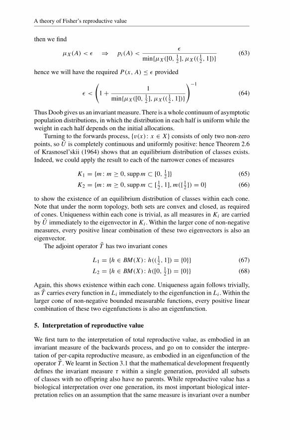
Thus Doob gives us an invariant measure. There is a whole continuum of asymptoticpopulation distributions, in which the distribution in each half is uniform while theweight in each half depends on the initial allocations.

Turning to the forwards process, {v(x) : x ∈ X} consists of only two non-zeropoints, so U is completely continuous and uniformly positive: hence Theorem 2.6of Krasnosel’skii (1964) shows that an equilibrium distribution of classes exists.Indeed, we could apply the result to each of the narrower cones of measures

K1 = {m : m ≥ 0, supp m ⊂ [0, 12 ]} (65)

K2 = {m : m ≥ 0, supp m ⊂ [ 12 , 1], m({ 1

2 }) = 0} (66)

to show the existence of an equilibrium distribution of classes within each cone.Note that under the norm topology, both sets are convex and closed, as requiredof cones. Uniqueness within each cone is trivial, as all measures in Ki are carriedby U immediately to the eigenvector in Ki . Within the larger cone of non-negativemeasures, every positive linear combination of these two eigenvectors is also aneigenvector.

The adjoint operator T has two invariant cones

L1 = {h ∈ BM(X) : h(( 12 , 1]) = {0}} (67)

L2 = {h ∈ BM(X) : h([0, 12 ]) = {0}} (68)

Again, this shows existence within each cone. Uniqueness again follows trivially,as T carries every function in Li immediately to the eigenfunction in Li . Within thelarger cone of non-negative bounded measurable functions, every positive linearcombination of these two eigenfunctions is also an eigenfunction.

5. Interpretation of reproductive value

We first turn to the interpretation of total reproductive value, as embodied in aninvariant measure of the backwards process, and go on to consider the interpre-tation of per-capita reproductive measure, as embodied in an eigenfunction of theoperator T . We learnt in Section 3.1 that the mathematical development frequentlydefines the invariant measure τ within a single generation, provided all subsetsof classes with no offspring also have no parents. While reproductive value has abiological interpretation over one generation, its most important biological inter-pretation relies on an assumption that the same measure is invariant over a number

A. Grafen

of generations. Essentially we will assume in this discussion that the population weare discussing maintains the same relative distribution of classes over time.

We defined an ‘ergodic set’ in Section 4.4 as a set A of classes such that allancestry of A belongs to A, and no other ancestry belongs to A (except perhapsfrom classes that have no descendants themselves in the long term, the ‘dissipa-tive’ classes). A minimal ergodic set has no proper subsets that are also ergodic.We saw that a minimal ergodic set has a unique invariant measure. The biologicalinterpretation is to pick an individual, and then one allele within that individual,in one generation, and find the distribution of the allele’s ancestors over classesin a large set of consecutive distant generations. If the generations are sufficientlynumerous and sufficiently distant, then the distribution of the ancestors across clas-ses can be represented as a probability distribution or measure over the classes.Two alleles picked from the same minimal ergodic set will give rise to the sameancestral measure.

If the whole of X is a minimal ergodic set, then this unique measure thereforeestablishes completely the relative values of all the different classes as ancestorsof distant generations. Some subsets of classes, such as sterile workers, may evenhave measure zero. This justifies the name ‘reproductive value’, and shows theimportance of the concept in natural selection. The Price equation (22) shows thatwhat happens to a class of individuals has a significance for natural selection thatis proportional to its reproductive value, and that individuals are selected to valueoffspring according to their per-capita reproductive value.

Now suppose there is more than one minimal ergodic set. We modify ourthought-experiment by choosing the individual and one of its alleles through somerandom process. If by this process the chosen allele might come from more thanone ergodic set, then the distribution of the ancestral state will be some mixture ofthe invariant measures for each minimal ergodic set, and by choosing the probabil-ities appropriately, we can obtain any convex combination of the unique invariantmeasures. Thus the family of invariant measures are all those measures which canprovide the distribution of distant ancestry from some given process of randomchoice of an allele in an individual in this generation.

The non-uniqueness arises because ancestry provides no way to establish therelative importance of two subsets of classes whose ancestry never intersects. Thusall distinct relative importances produce distinct invariant measures. Such subsetsare as separate as different species, because there is no gene flow among them.An extreme caste system, or complete geographical separation, could in principleproduce such subsets within a species.

However, not all of these invariant measures will fulfil the fourth and crucial roleof reproductive value, namely as a maximand of adaptive evolution. Explicit linksto optimisation programs are made in parallel papers (Grafen, 2002, 2006), wherethere is enough work to do with them to justify introducing the notation. Explicitoptimisation is also shown in the examples in Section 8, where less general resultsare required. Here, an example will show why not all invariant measures producea maximand. Suppose there are two classes x and y, and an individual producesexactly one offspring of its own class and none of the other. The two classes per-petuate themselves and remain in equilibrium. Then the invariant measure τ can

A theory of Fisher’s reproductive value

place an arbitrary weighting on x and the remainder on y, for whatever chances weplace on choosing classes in the offspring will be the chance that the parent is ofthose classes. But further suppose that a class x parent has the option of producing0.7 class y offspring, and that a class y parent could produce 0.9 class x offspring,but that neither of these options is taken up at equilibrium. Then τ({x}) and τ({y})are the class reproductive values, and µX({x}) and µX({y}) are the masses ofindividuals in the classes. It follows that the per-capita reproductive values are

h(x) = τ({x})µX({x}) and h(y) = τ({y})

µX({y}) (69)

The two classes of parents are acting optimally in continuing to produce their ownkind only if these conditions hold

h(x) ≥ 0.7h(y) (70)

0.9h(x) ≤ h(y) (71)

This would limit the ratio of per-capita reproductive values to lie between 7/10 and10/9. In general, all options not taken up will place restrictions on which of theinvariant measures produce maximands.

Is it possible that this kind of argument might rule out all of the invariant mea-sures? Indeed it is, and will occur when the behaviour is not optimal. Let us amendthe previous example, and suppose that an individual in class x could have made2.5 offspring in class y, while an individual in class y could still make 0.9 offspringin class x. Then the optimal behaviour would be for each class to make the other,producing a higher rate of increase for each lineage, growing by a ratio of 1.5each generation compared to the static population of the original phenotype. It isappropriate that none of the invariant measures will produce a maximand.

We now turn to the interpretation of per-capita reproductive values as repre-sented by a solution h to equation (26), and restrict ourselves initially to the casewhere there is only one minimal ergodic set in X. In populated regions of X, h(x)

is just the total reproductive value of class x, divided by the population size at x.This ratio is however undefined in unpopulated regions, and yet h has a crucialinterpretation there. Suppose we begin with an individual at x. Then we know fromthe invariant measure what the class-distribution of its descendants will eventuallybe, and h(x) represents how many of those descendants there will be.As individualsin every class x produce the same eventual class-distribution, h(x) represents theratio of the numbers of descendants produced by adults at each x. The significanceof this extension beyond populated regions arises when considering the fate ofmutants with low penetrance. A mutant may cause an individual to place offspringoutside the populated regions, but because of the low penetrance, the descendantsof those ‘outsiders’ will have regained the populated regions before the deviantbehaviour occurs again. The value of h(x) for those outsider offspring evaluatestheir descendants, as shown formally in equation (27). Thus the wider definitionof per-capita reproductive value is essential when dealing with mutants that placeoffspring outside the regions populated by the common phenotype.

A. Grafen

It is important to stress that total reproductive value and per-capita reproductivevalue depend on different information. Total reproductive value, embodied in theinvariant measure τ , is obtained from information on w(i) alone, that is, from infor-mation about the classes that are occupied. By contrast, the per-capita reproductivevalue h depends on knowing v(x) for all x, which includes what would be done byindividuals in unoccupied classes. The per-capita reproductive value in unoccupiedclasses must be calculated from assumption, as ‘observation’ can produce only theundefined quotient zero divided by zero.

6. Equilibrium under natural selection with classes

The existence of classes creates a question about how evolutionary equilibrium isto be defined. Two possibilities are described in this section, and then using thesecond, two important results are proved about natural selection in the presence ofclasses.

6.1. Clonal growth

The simplest approach is based on the idea of a completely dominant allele, whichbrings about a new phenotype in every bearer. The bearers thus grow as a clonewould, and the complication of classes means keeping track of the distribution ofthe clone over the classes, and finding its intrinsic growth rate. The key point is thatwhen averaging across the new strategy’s success in the different classes, the aver-age is weighted by the distribution of classes brought about by the new strategy’sown behaviour.

We therefore define a Markov operator Ua : M(X) → M(X) to represent theevolution over one generation of the distribution over X of a clone of a-strategistswhose distribution of offspring classes is given by va . Formally,

Ua(m) =∫

va(x)m(dx) (72)

The spectral radius of the operator will be denoted ρ(Ua). In fact this operator isthe operator U of the forwards process, but recognising the dependence on a givenphenotype a.

If we assume that the population as a whole is at a putative equilibrium and hasreached a stable population density with monomorphic strategy a, then a conditionfor equilibrium is that no strategy could spread, formally that ρ(Ub) ≤ ρ(Ua) forall feasible strategies b. This inequality can be used as the basis for an optimisationprogram with the spectral radius as maximand. See Grafen (1998) for an exampleof such an optimisation program, but in a simpler case with finite X.

Reproductive value plays no obvious role in this equilibrium concept.

6.2. Stubblefield’s ‘tracer-allele’ method

The alternative approach (Seger & Stubblefield, 2002) is to consider a mutant thathas very low penetrance. Thus, it plays the existing strategy most of the time, and

A theory of Fisher’s reproductive value

occasionally plays a new strategy. The difference this makes is that the new strat-egy is played in a distribution of classes that corresponds to the distribution of thepopulation as a whole, rather than the distribution that would come about throughthe actions of the new strategy itself.

As the mutant is played in the same distribution of classes as the population, ap-score is selected according to the sign of Iτ (π

′ − π). Recall from equation (21)that

Iτ (π′ − π) = E

[p(F

τWw − E

[F

τWw

∣∣χ])] (73)

If a population is such that no p-score would spread, it follows that the right handfactor in the expectation must equal zero as a member of L1(µI , R), and the con-verse also holds. Formally,

FτWw = E

[F

τWw

∣∣χ] ⇔ no p-score can spread (74)

The interpretation is simple: there is no natural selection exactly when each individ-ual has the same scalar evaluation of its reproductive output as the other individualsin the same class (apart from a possible set of individuals of measure zero). This isthe formal statement for an arbitrary set of classes as was noticed for finite classesby Fisher (1930), Taylor (1990) and others, to the effect that if fitness differencesare related to class but not to phenotype, then weighting by reproductive valuegives no net selection. With any other weighting, two alleles with identical pheno-typic effects could be differentially selected simply as a result of being distributeddifferently over the classes.

Equation (74) is the condition that all extant phenotypes should be in selectiveequilibrium, which in the parallel analysis without classes Grafen (2002) calls ‘noscope for selection’. The ‘potential for selection’ is measured by the success of anon-extant phenotype a that usually produces the same offspring distribution v asthe population as a whole, but with very low probability produces the distributionva . Assuming that the descendants return to the population distribution before themutant is expressed again, we can use equation (27) to write the condition that nosuch mutant could spread:

for all feasible mutants a∫∫h(y)va(x)(dy)µX(dx) ≤

∫∫h(y)v(x)(dy)µX(dx)

(75)

The implications depend very much on the set of possible mutants. The generalexpression allows arbitrary constraints that link behavior in different classes; but ifbehaviour in all classes can evolve separately, then we have the simpler

for all feasible mutants a and classes x∫h(y)va(x)(dy) ≤

∫h(y)v(x)(dy)

(76)

These are the two basic results for selection in the presence of classes.

A. Grafen

6.3. Comparison of the concepts

The logical basis of the difference between the clonal growth and tracer-alleleequilibrium concepts is how they weight the classes when averaging the effects ofphenotypes across the different classes. Clonal growth assumes the mutant allelehas the distribution over phenotypes produced by a clone showing the mutant strat-egy, whereas a mutant allele will usually have a more complex relationship to themutant strategy: to give only two simple examples from diploid genetics, it couldbe a recessive allele or it could show partial penetrance. Even a dominant allelewould deviate from the clonal case once it was frequent enough for homozygotesto arise. Tracer-alleles assume that the mutant allele’s distribution over classes isidentical to the population’s existing distribution. While this would follow fromextremely low penetrance, or from a simple constant factor of advantage in repro-duction in all circumstances per copy of the allele, it is otherwise most unlikely.Other distributions of the mutant allele over classes are highly likely to be relevantin real cases. However, these are two natural possibilities that have been used in theliterature (Seger & Stubblefield, 2002). In the rest of the paper, it is the tracer-allelemethod that will be employed.

There are reconciliatory conditions in which these conditions are the same formutants close to the incumbent, and Grafen (1998) gives an example in which thetwo conditions are equivalent for all mutants when a population is at a selectiveequilibrium.

The tracer-allele approach is more convenient to apply in evolutionary modelsbecause once reproductive values h(x) have been worked out under the incumbentphenotype, a simple weighting of offspring classes allows the evaluation of the suc-cess of any mutant phenotype, so long as we are willing to assume low penetrance.This implies a simple trade-off between offspring classes that is the same for adultsin every class, and that can be applied in one aspect of the phenotype independentlyof choices in other aspects.

There is a general biological defence of using the tracer-allele equilibrium con-cept to investigate the effects of selection on phenotypic traits. This concept useslittle information about genetics, but nevertheless allows results to be obtained.Full population genetic models use more information, and clearly some full geneticmodel must be right in any particular situation. The main difficulty with full modelsis that the extra genetic information will usually be unknown in any particular case,and furthermore will also be different in every particular case. For example, a modelabout sex ratio using the tracer-allele concept provides admittedly tentative results,but they apply to a wide variety of species. A full model would require informa-tion that was different for each species, and even if the information were available,would produce predictions that were different. Thus the approximate applicabilityof the tracer-allele concept is close to a necessary condition for general biologicalexplanations. If genetic details are truly required, then such general explanationsdo not exist. The optimisation programs attached to the phenotypic concepts alsoprovide an interpretation of the conclusions that makes sense of the biology.

The argument between game theorists and population geneticists over the rel-ative value of strategic models and explicit genetic models cannot be reviewed

A theory of Fisher’s reproductive value

here, and will certainly continue. A major purpose of the formal Darwinism project(Grafen, 2002, 2006, and the present paper) is to put the strategic models on anequal footing in terms of mathematical rigour, so that choices can be made on thegrounds of biological utility.

The next two sections apply the tracer-allele approach, first to expound Fisher’suse of reproductive value, and then to apply the mathematical machinery developedin this paper to some examples.

7. Fisher’s four uses of reproductive value

One principle aim of the paper is to make explicit Fisher’s concept of reproduc-tive value as an evolutionary maximand. In this section, which is intended to beaccessible to biologists with only a little mathematical notation, Fisher’s uses ofreproductive value in his 1930 book are reviewed. Page numbers are taken from theVariorum edition published in 2000. Then the links are made to the formalism estab-lished in earlier sections. The reader is reminded that reproductive value assigns anumerical value to individuals and to subsets of the population, representing theirimportance in evolutionary processes.

Fisher first employs the concept on pages 27 to 29 in relation to the Euler equa-tion and age-structured populations (for a more recent treatment see Charlesworth,1994). On page 29, he makes the point, in the same context, that using reproductivevalue appropriately over one generation is the equivalent of looking an indefinitenumber of generations ahead in order to obtain an asymptotic measure of fitness.In deriving the fundamental theorem of natural selection, he asserts on page 35 thatindividuals should be weighted by their reproductive value when gene frequenciesare measured. On page 73, Fisher declares in comparing the strength of naturalselection in larvae and adults first that one should count not number of bearers butrather their summed reproductive value, and second that weighting by reproductivevalue in this way brings about comparability between the two groups.

The only explicit use as a maximand comes in pages 141 to 143 in the famoussex ratio argument, but here many logical steps are taken. The total reproductivevalues of all males and of all females are calculated, and then the per-capita repro-ductive values. These are attributed as the value of a son and a daughter, and thesum of the shares of a parent in the reproductive values of its offspring is identifiedwith the reproductive value of the parent itself. It is then assumed that selection willcause this reproductive value to be maximised within the actions available to theindividual. Further, uncertainty is taken into account when the probability-weightedarithmetic average is taken over possible reproductive values.

The various manipulations exhibit a sophisticated if implicit structure. It is nowshown how the machinery of the present paper provide formal justifications formost of these manipulations, and in a very general setting. The exception is aver-aging over uncertainty, which must be deferred. Reproductive value is thus shownto be a central concept in natural selection in the presence of classes.

Fisher (1930) used reproductive value in four formal ways that are illustrated bythe roles played by reproductive value in the Price equation with classes. Equations

A. Grafen

(22) and (23) are expressed in terms of h as follows:

∫h(x)

(π ′(x) − π(x)

)µX(dx) = E

[C[p,

∫h(x)w(·)(dx)

∣∣ χ]]

(77)

∫h(x)

(π ′(x) − π(x)

)µX(dx) = C

[p − E [p | χ ] ,

∫h(x)w(·)(dx)

](78)

The equations need to be explained for readers who have skipped the mathe-matical sections, who can understand ‘p-score’ to mean ‘gene frequency’. h(x) isthe per-capita reproductive value of an individual in class x. π ′(x) and π(x) arethe mean p-score next generation and this generation among individuals in classx, and µX represents the population distribution over classes in the parental gen-eration. Thus the left hand side represents a population-wide average change inp-score from this generation to the next, weighting by reproductive value. On theright hand side, the integral represents the reproductive-value-weighted evaluationof one individual’s production of offspring – or more accurately, of her appropriateshare of them, according to the fraction of each offspring’s genes she contributed.The first right hand side is the average over classes of the covariance across indi-viduals within a class between p-score and that integral. The second right hand sideis the covariance over all individuals between the deviation of p-score from classmean p-score, and that integral.

Fisher’s first and second uses are that reproductive value provides the weightsin aggregating gene frequencies into a single gene frequency, either by individualweight or by class weight. The use of h is in the left hand side of equations (77) and(78), where h(x) is the weight of an individual in class x and h(x)µX(dx) is thetotal weight of class x. These weights have the special property that when there isno selection within classes, indicated by the covariances in the right hand sides alltaking the value zero, there is no change in the mean gene frequency. Aggregatinggene frequencies must be done with very special weights to have this property, andthis is one of the important properties of per-capita reproductive values (this resultis shown formally in Section 6.2).

The third use is in the construction of an individual’s reproductive value, whenreproductive values are used to weight the sum of shares of offspring produced ofeach class. This is shown in the right hand sides of equations (77) and (78), whereh(x) is used to weight the gametic contributions by an individual to offspring oftype x.

The fourth use of reproductive value is as a maximand, a function individualsare selected to maximise. This use can be seen in the position of the individual’sweighted sum of its shares in the reproductive values of its offspring, as the tar-get of selection in the Price equation (77 and 78). This corresponds to the roleof number of offspring in the standard Price equation (Price, 1970), to expectedrelative number of offspring in the Price equation with uncertainty (Grafen, 2002),and to expected relative inclusive fitness in the Price equation with uncertainty andeffects on relatives (Grafen, 2006). Once there are various classes of offspring,then aggregation is required to find a single maximand. It is the combination ofweighting gene frequencies by reproductive value, and summing offspring number

A theory of Fisher’s reproductive value

weighted by reproductive value, that allows the conclusion that a p-score positivelycorrelated with aggregated offspring number will increase.

So far the target of selection has been the sum of the parent’s shares in its off-spring’s reproductive value. In view of equation (26), which defines reproductivevalue in a uniform population as the sum of its shares in the reproductive value ofits offspring, we can understand the parent’s own reproductive value as the targetof selection, and regard it as a generalisation of counting offspring, giving weightsaccording to class.

The second major result can also be interpreted in Fisherian terms. This is thecondition for a strategy with reproductive output v to be proof against invasion: forall feasible mutants a∫∫

h(y)va(x)(dy)µX(dx) ≤∫∫

h(y)v(x)(dy)µX(dx) (75, repeated)

Each side is a double integral that first adds up the reproductive value of offspringof an individual in class x, and then adds those up weighting by the distribution ofadults in the different classes, yielding a total reproductive value for va on the left,and for v on the right. This clearly shows that to be uninvasible, v must attain themaximum of that double integral, over feasible possibilities. The optimisation ofreproductive value as a condition for evolutionary equilibrium, used by Fisher inhis sex ratio argument, is thus exhibited formally.

For both results, weighting by per-capita reproductive value reduces the pos-sible complexity of classes considerably. Offspring classes each have a weight,and the quantity to be maximised is the sum of those weights over the offspringproduced. Thus there is a simple tradeoff between all pairs of offspring classes,and furthermore that tradeoff is the same for all parental classes. The formalismtherefore shows how the assumption of low penetrance, and the assumption of onecommon type faced with possible rare mutants, together simplify the operation ofnatural selection in the presence of classes and permit a simple optimisation view.

Fisher nowhere gives a formal argument for employing reproductive value asa maximand when there are classes present in the population. The Price equation,however, provides a framework in which reproductive value plays a central role,and which unites and fully justifies Fisher’s various uses of the concept in a verygeneral setting.

8. Examples

The examples in this section show the theory at work. The first example is Fisher’ssex ratio argument. We follow Taylor (1990) in providing a treatment in which thederivation and application of reproductive value are fully included in the formalarguments. The power of the theory is shown by various extensions. The secondmodel is of parental care, in which resources are distributed to individuals on thebasis of size. A technical point here is a further result of Rosenblatt (1971), extend-ing his condition to non-compact X. The third example is geographical.

In the examples, we shall assume in the notation of Section 4 that the populationmeasure over classes is µX, and that the aggregate production of offspring over X

is V .

A. Grafen

Optimisation programs are introduced explicitly here. It is convenient to statehere without proof two very simple results about linear programming in infinitedimensions. The literature (e.g. Luenberger, 1997; Anderson & Nash, 1987) seemsto provide no simple and suitable general results, as it is concerned with morecomplicated problems.

For the first result, we assume Y is compact Hausdorff which with its Borel setsforms a measurable set, K > 0, and f, g are measurable functions from Y to R

satisfying f ≥ 0, f �= 0 and g(x) > 0 for all x. Consider the optimisation programfor non-negative finite real measures over Y ,

µ max∫

f (x)µ(dx),

∫g(x)µ(dx) ≤ K (79)

Let λ = sup{f (x)g(x)

} ∈ (0, ∞]. Then we claim that

µ

({x :

f (x)

g(x)= λ

})=µ(Y )⇔Lµ solves program (79) for some scalar L > 0

(80)

Note that this result requires measurable functions f and g defined everywhere,and not merely belonging to some L1; and I am grateful to Dr Matthew Daws forthe observation that the set of maximising values is measurable as it is the inverseimage of a measurable set under a measurable function.

For the second result, we assume Y is compact Hausdorff which with its Borelsets forms a measurable set, µ is a positive real finite measure on Y , f ∈ L1(µ, R),f ≥ 0, f �= 0, and K > 0. Consider the optimisation program for instrumentsk ∈ L∞(µ, R)

k max∫

f (x)k(x)µ(dx),

k(x) ≥ 0

k(x) ≤ 1∫k(x)µ(dx) ≤ K (81)

Then let Q(c) = {x : f (x) > c} and R(c) = {x : f (x) = c} . Then µ(Q(c))

and µ(Q(c) ∪ R(c)) are non-increasing functions of c. Suppose µ(Q(0)) ≥ K .Let c∗ = inf{c : µ(Q(c)) < K}. Then we claim that a necessary and sufficientcondition for k to be a solution to the program (8.1) is

∫k(x)µ(dx) = K and µ-a.e.

k(x) = 1 x ∈ Q(c∗)0 ≤ k(x) ≤ 1 x ∈ R(c∗)k(x) = 0 x /∈ Q(c∗) ∪ R(c∗)

(82)

Armed with these results, we now tackle three examples.

A theory of Fisher’s reproductive value

8.1. A sex ratio model

The only model in which Fisher explicitly used reproductive value as a maximandwas his sex ratio argument. Edwards (1998) claims that the argument was notoriginal with Fisher. The reproductive value aspects to be brought out in the presenttreatment show a central part of the rigorous argument which I do not believe wasmade before Fisher in 1930. In particular, the need to show that the reproductivevalue of all males equalled the reproductive value of all females, and indeed theconceptual framework in which such a statement can even be formulated, were notto my knowledge appreciated by earlier authors. Until Mendel’s results becamewidely known, biologists did not know the crucial fact for this argument that thetwo parents contribute equally to each offspring, and indeed this is not true forsex chromosomes in diploids, or at all for haplodiploids. It is at least possible thatDarwin (1871) withdrew his sex ratio argument in making the second edition ofthe Descent of Man because he saw this lacuna in the argument of the first edition.

It is fitting to begin by making Fisher’s argument of equal total reproductivevalues. The situation is one in which the sexes are distinct and parents choose thesex of offspring. Class therefore determines sex, and so we may write the sets ofmale and female classes as M and F , with M ∪ F = X and M ∩ F = ∅.

Making the same assumption as Fisher that each offspring receives equal con-tributions from a father and a mother, it follows that the total reproductive output ofmales equals the total output of females, where the equality holds for the whole dis-tribution across classes. We require to show that this equality of total reproductiveoutput implies equality under the invariant measure τ , or formally

∫M

v(x)µX(dx) =∫

F

v(x)µX(dx) ⇒ τ(M) = τ(F ) (83)

We will prove that this must be true on the supposition that τ is an invariant measure,without proving that one exists. By definition an invariant measure satisfies

Iτ f = Iτ Tf ∀f ∈ L1(V , R) (84)

By definition, Tf = DV E [f v]. Let us choose f to be in turn fM and fF , theindicator functions of M and F . Then we have

τ(M) = Iτ fM = Iτ DV E [fMv] = Iτ DV

∫M

v(x)µX(dx) (85)

τ(F ) = Iτ fF = Iτ DV E [fF v] = Iτ DV

∫F

v(x)µX(dx) (86)

But the final term in each line is equal by the hypothesis of equation (83), and sowe have as required that τ(M) = τ(F ). Thus Fisher’s equality result is true in anextremely general setting.

The equality result just obtained will be used below, but first we show howthe argument can be generalised beyond simple diploidy, and study the ‘arbitraryploidy’ model of Grafen (1986), which includes diploidy, haplodiploidy and hap-loidy as special cases. Assume that all males share the same ploidy and all femalesshare the same ploidy, but these may be different. Females contribute γFF -ploidgametes to daughters and γFM -ploid gametes to sons. Males contribute γMF -ploid

A. Grafen

gametes to daughters and γMM -ploid gametes to sons. We aim to find the classreproductive values of females and males, still retaining the assumption of discretenon-overlapping generations.

Define k ∈ L1(V , R) by k = DV

∫F

v(x)µX(dx). Then k(y) equals the frac-tion of successful gametes in type y offspring that come from females. The ploidyassumptions show we must have

k(y) ={

γFF

γFF +γMFy ∈ F

γFM

γFM+γMMy ∈ M

(87)

We apply the definition of invariance for τ to the indicator function fF , to obtain

τ(F ) = Iτ DV

∫F

v(y)µX(dy) = Iτ k (88)

= γFF

γFF + γMF

τ(F ) + γFM

γFM + γMM

τ(M) (89)

showing that

τ(F )

τ(M)=

γFM

γFM+γMM

γMF

γFF +γMF

(90)

which has a nice interpretation in words as

reproductive value of all females

reproductive value of all males= fraction of male genome from mother

fraction of female genome from father(91)

This argument includes haplodiploidy with γFF = γFM = γMF = 1 andγMM = 0. Note that, as with the simple diploidy result, the results hold even ifthere are subclasses within F and M with their own further subdivisions of repro-ductive value. This result confirms that of Grafen (1986), obtained with informalmethods.

8.1.1. Fisher’s original argumentIn Fisher’s original argument, X = M ∪ F and M and F have one element each.A parent’s production of male and female offspring, g(M) and g(F ), was limitedby the investment required according to a linear constraint of the form cMg(M) +cF g(F ) ≤ K , where the per-capita costs are cM and cF . The total reproductivevalues of males and females are equal to each other, as we have just seen, and soequal to 1

2 . We make explicit Fisher’s implicit assumption that we are consideringa rare mutant in a very large population whose incumbent strategy is not changingfrom one generation to the next. The per-capita reproductive values are therefore

1

2µX(M)and

1

2µX(F)(92)

A theory of Fisher’s reproductive value

The optimisation program for an individual choosing offspring numbers is therefore

g(M), g(F ) maxg(M)

2µ(M)+ g(F )

2µ(F),

g(M) ≥ 0

g(F ) ≥ 0

cMg(M) + cF g(F ) ≤ K (93)

We introduce Lagrangean multipliers λ, γM and γF , and the Lagrangean itself as

L = g(M)

2µ(M)+ g(F )

2µ(F)+ γMg(M) + γF g(F ) − λ(cMg(M) + cF g(F ) − K)

(94)

The Lagrangean is unconstrainedly maximised by the instruments, and the resourceconstraint will always be met with equality. Thus we write the conditions for a con-strained optimum as

1

2µ(M)− λcM + γM = 0 C.S.

{γM ≥ 0

g(M) ≥ 0(95)

1

2µ(F)− λcF + γF = 0 C.S.

{γF ≥ 0

g(F ) ≥ 0

where C.S. denotes complementary slackness (i.e. at least one inequality holds withequality).

As is typical in ESS and optimality arguments, we are going to use propertiesof the maximisation to draw conclusions not about the maximising response, butabout the population values µX(M) and µX(F). If all individuals have the samecosts, then their solution to this optimisation program will be the same. If γM > 0,then by complementary slackness no males are made by optimising agents, whichprecludes an equilibrium. Thus at an equilibrium we must have γM = 0 and by aparallel argument γF = 0. Then the equality conditions can be used to eliminate λ

and obtain

µ(M)

µ(F)= cF

cM

orcMµ(M)

cF µ(F )= 1 (96)

The first version states that the sex ratio in numbers is the ratio of costs, and thesecond that the sex ratio in investment is equal.

This is one of the most famous arguments in evolutionary biology, and therehave been many formal and informal versions with the same conclusion. The argu-ments are reviewed by Edwards (1998) and Seger & Stubblefield (2002), and seealso Edwards (2000) for a fascinating historical discovery. Most authors have madeonly informal links between reproductive value methods and rigorous populationgenetics in sex ratio arguments, and Seger & Stubblefield (2002) present them as

A. Grafen

distinct and complementary. However, the two approaches were explicitly and for-mally bridged by Taylor (1996, uncited by Seger and Stubblefield), who thereforeprovided the first rigorous version of the reproductive value argument. The presentpaper extends this by permitting a further class structure within each of the sexes,which we proceed to exploit.

One more sex ratio model needs to be mentioned here. Leimar (1996) presenteda formal version of the verbal model of Trivers & Willard (1973), and solved inthat case many of the technical problems being encountered here. The Trivers-Wil-lard model is perhaps the most prominent evolutionary idea which requires such acareful handling of reproductive value, and Leimar’s work shows the importanceof taking the formal approach.

8.1.2. An extensionNow suppose class is the Cartesian product of {M, F } and [a, b], with 0 < a < b,and that the population of females on [a, b] is represented by the finite measure φf

and of males by the finite measure φm. We first discuss the monomorphic popula-tion against which mutants will be tested. Suppose females choose the sex of theiroffspring and all make the same relative distribution of classes within each sex,which must therefore be proportional to φf and φm, but may vary in their magni-tudes. We will come back to the question of whether it might be advantageous forfemales of different classes to make different relative distributions. We also assumethat females are constrained in offspring production measures gf and gm by theirown parental class x such that∫

ygf (dy) +∫

ygm(dy) ≤ Kx (97)

so that it costs y to make an individual of class y, and class is advantageous to afemale in allowing her to make more offspring. Suppose that male classes mateindependently with female classes, and that the mating success of males in class y

is proportional to y2. Then as individuals of each sex make offspring in sex-spe-cific proportions across the classes, but differ only in the absolute numbers, we canstraight away define the invariant measure τ = τf + τm in its two components forfemales and males, respectively, by

τf (A) = 1

2

∫A

yφf (dy)∫yφf (dy)

τm(A) = 1

2

∫A

y2φm(dy)∫y2φm(dy)

(98)

and the per-capita reproductive values by

hf (y) = 1

2

y∫yφf (dy)

hm(y) = 1

2

y2∫y2φm(dy)

(99)

The evolutionary maximand is therefore incarnated, neglecting for conveniencethe fixed factor of 1

2 , as∫

ygf (dy)∫yφf (dy)

+∫

y2gm(dy)∫y2φm(dy)

(100)

with the constraint for an individual female in class x represented by equation (97).

A theory of Fisher’s reproductive value

We now employ the result (80), in whose terms for the males, we have f (x) =y2/

∫y2φm(dy) and g(x) = y. The ratio f (x)/g(x) is therefore y/

∫y2φm(dy).

As y is positive, only the highest value of y can attain a maximum, and so if malesare made at all in the optimal solution, then we must have gm place all its measure ony = b, so that the value of λ is b/(b2φ({b}) which equals 1/(bφ({b}). The femaleratio is 1/(

∫y2φf (dy)) and thus independent of y, so either all female classes or

no female classes may be produced at the optimum. We are interested in values ofφf and φm that might be optimal, so we require that both females and males aremade. Thus the ratio for females must equal the ratio for the only permitted maleclass, showing that ∫

yφf (dy) = bφm({b}) (101)

These terms are respectively the total investment in female and male offspring, andso we have established from first principles Fisher’s equal investment result in thiscontext. It is a necessary and sufficient condition for optimality that only b-malesbe produced and that the investment in both sexes be equal.

This implies that the ratio of different classes as shown in the relative valuesof φf is irrelevant to female reproductive value, so φf may contain atoms andgaps. The optimisation result shows there is no selection to deviate from the givenallocation by females to different classes. This is not surprising, as the only advan-tage to a class for females is its ability to invest, and that ability is proportionalto the investment in it. Thus there are equal per-investment returns and the size ofthe unit is immaterial. This answers in the negative the question posed earlier ofwhether it might be advantageous for females in different classes to choose a differ-ent distribution of offspring. (This does leave open the possibility that if femaleswere polymorphic for φf , there would be a different outcome of selection, but weneglect that here.)

This treatment of a sex ratio problem has illustrated how Fisher’s argument canbe extended using the formalism developed in the paper. We have both indifferencebetween investment classes for the females, and an atom showing all males areproduced into the same class. These are useful kinds of outcomes to be able tohandle.

The tools used here might well with mild extensions allow the development ofa complete justification of the reproductive value approach to sex ratio problemsfrequently used in biology, and as formalised for example by Boomsma & Grafen(1991).

8.2. Rank order for resources, and a non-compact X

We now turn to a parental investment model, in which an amount x is invested toplace an offspring in class x ∈ [a, ∞) with a > 0. Resources among the offspringare awarded on a competitive basis, such that only the rank of the offspring by classmatters. Specifically, per-capita resources for class x, r(x), are determined so that

∫ ∞

x

r(x′)m(dx′) =√∫ ∞

x

m(dx′) (102)

A. Grafen

where the total resources are therefore 1. We differentiate with respect to x to obtain

r(x) = 1/(2√

m({[x, ∞)}) (103)

The minimum per-capita resource is therefore 12 for the lowest class, but it rises to

∞ for the highest class.Consider an individual in class x who has resources r(x) and produces a mea-

sure g across offspring classes, and so is subject to the constraint∫

yg(dy) ≤ r(x).As the maximand and constraint are proportional, it is clear that the per-capitareproductive value must be proportional to r(x) so the invariant measure τ willsatisfy τ(dx)/m(dx) = κr(x) for some κ > 0. Thus we can write the maximandas∫

r(y)g(dy), and the program is

g max∫

r(y)g(dy),

∫yg(dy) ≤ K (104)

It follows from result (80) that for classes y produced in an optimal solution,we must have λ = r(y)/y. Standard arguments (e.g. Bishop & Cannings, 1978)show gaps cannot be optimal if they have an upper bound (the same resources areavailable at a lower cost), and the infinite per-capita resource shows that the supportof an optimal solution cannot have an upper bound. Thus we find the populationmeasure that ensures λ = r(y)/y for the whole interval [a, ∞), which is

m(dy) = 2a2

y3 dy (105)

The space of classes X is not compact, but nevertheless, the existence of τ isnot in doubt in this example. However, a further result of Rosenblatt (1971, page104), beyond that discussed in Section 4.3, is worth mentioning in this context fora measure space based on a metric space X, its Borel sets X and a measure µ. Inplace of compact X, and T taking continuous functions to continuous functions,we may instead have locally compact X, and T taking bounded continuous func-tions to bounded continuous functions. An additional requirement is that there is acompact subset of X through which the trajectory of each point x ∈ X passes withprobability one. Then the theorem tells us that there exists an invariant measurewhich is sigma-finite. This means there is an at most countable subset of X whoseunion covers X, and over each element of which the measure is finite.

The condition of trajectories passing through a compact subset refers to a tra-jectory of ancestors in the biological case. It states that there must be a compactset such that for every individual lying outside that set, the probability that theirancestral path at no point intersects the compact set is zero. In this example, eachindividual has an equal finite chance that its immediate ancestor lies in [a, a + 1],so the probability that at least one ancestor lies in [a, a + 1] is indeed one.

A theory of Fisher’s reproductive value

8.3. A geographical example

Suppose X represents geographical space, which may be a compact subset in one,two or three-dimensional space, that µ represents the Borel measure, and that thereis another measure p over X representing the rate at which a region can produceoffspring. The total productivity of a region A is fixed by p(A), and shared amongthe µX(A) individuals present there. The offspring produced may be distributedin space, and we suppose that the common strategy is represented by a functions(x, y) which equals 1 if parents at x produce offspring at y, and 0 otherwise. Wedefine sets of the parents that produce given offspring and the offspring producedby given parents as follows:

P(y) = {z : s(z, y) = 1} O(x) = {z : s(x, z) = 1} (106)

We make two further assumptions about reproduction. We assume that parents atx produce offspring evenly over O(x), and that offspring are spread over a regionwhose Borel measure (area in two dimensions) is a constant β−1 for all parents.Thus

v(x)(dy) ={

βp(dx)

µX(dx)µ(dy) y ∈ O(x)

0 y /∈ O(x)(107)

β−1 = µ(O(x)) =∫

s(x, y)µ(dy) > 0 (108)

This allows us to write (Tf )(y) as

(Tf )(y) = (DV E [f v]) (y) = β

∫P(y)

f (x)p(dx)∫P(y)

p(dx)(109)

If the population reaches an equilibrium of class dynamics, then as each parentproduces a density there can be no atoms of population. We proceed on the basisthat there exists a function h representing the per-capita reproductive value of off-spring. We aim to find the optimisation program based on the choices of a particularindividual. Let e(y) be the indicator function of the set of locations within whichthat individual is free to place offspring, and let the strategy function be f . We canrepresent the program as

f max∫

e(y)f (y)h(y)dy,

∫f (y)dy ≤ K

f (x) ≤ 1

f (x) ≥ 0 (110)

This program can be solved using result (82). Thus an area Q with the highestvalues of e(y)h(y) is fully occupied, and an area R with the unique marginal valuec∗ of e(y)h(y) is occupied to the extent required to ‘use up’ the area an individualcan place offspring into.

A. Grafen

If e(y) is uniformly 1, so there are no restrictions on where individuals can placeoffspring, then this shows that the area of ‘super-normal profits’ is small enoughto be less than the area of one individual’s offspring. This provides what is veryclose to an ‘ideal free distribution’ (Fretwell, 1972), in which the distribution oforganisms matches the distribution of resources, and the per-capita reproductivevalues are equal. There is only a small exceptional area caused by the restrictionthat individuals cannot fully concentrate their offspring.

If e(y) differs between individuals, perhaps so that individuals can place off-spring only near to their own location, then the whole argument would become morecomplicated as the value of c∗ could vary from place to place. This example hasshown how the reproductive value methods developed in this paper can in outlinebe applied to geographical questions.

9. Comparison with Taylor

Taylor (1990) provided a theory of reproductive value for finite X. Here a compar-ison is made between Taylor’s theory and that of the current paper. There is oneimportant difference in emphasis. Taylor does not particularly link his results tothe work of Fisher (1930), whereas the whole of Section 7 shows how the resultsprovide a formal justification of an underlying structure in Fisher’s evolutionaryanalyses.

The formal differences will be discussed using the notation of the present paper.The first difference is that Taylor’s X is finite while here it is compact Hausdorff,which implies it can have continuous and discrete components and can be multi-dimensional. One advantage of this generality is that some examples, such as paren-tal care or location, might be more naturally modelled with continuous components.Even some infinite-dimensional sets could be handled, perhaps representing shape.Another advantage is that reproductive value is shown in a wider context to play anessential role in natural selection.

The second difference is that Taylor assumes a very simple diploid genetics,with a single locus with two alleles, one of which is a rare mutant; and restrictsattention to a one-dimensional space of phenotypes. Here initially a general genet-ics is permitted with arbitrary ploidy, in which the change in an arbitrary p-scoreis discussed, and the set of phenotypes is arbitrary. This allows multiple alleles atmultiple loci, and arbitrary epistasis and linkage. The main Price equation derivedby Taylor has the same form as here, in being an average over classes of a covariancewithin each class, but his equation (16) holds only to second order in the mutantfrequency, while here the main Price equation (equations 22 and 23) is exact inexpectation with arbitrary genetics. For some parts, notably Section 6 in discussingequilibrium, the present paper does move much closer to Taylor, assuming geneticuniformity apart from a rare mutant, and restricting attention to just two phenotypes.

Taylor does not discuss the ambivalence of equilibrium concepts discussed inSection 6, as he considers only the reproductive-value-weighted gene-frequencyas indicating success of an allele. In the 1990 paper, he permits the rare mutantto have an arbitrary phenotype, and states his results to first order in the mutantfrequency. This position neglects the possibility that the new phenotype might alter

A theory of Fisher’s reproductive value

its own class distribution so that the reproductive-value-weighted gene-frequencyis no longer a good measure of the success of an allele. In our terms, such a strategymight spread under the clonal growth condition but not under the tracer-allele con-dition. In 1996, Taylor makes the additional assumption that the mutant phenotypeis very close to the common phenotype, and so resolves this difficulty.

Taylor (1996) does however have a different distinction to draw, between mutantstability (whether a fixed population is stable against a small population of mutants)and population stability (whether a population slightly displaced as a whole froman equilibrium induces selection pressures that tend to restore the original state).From a formal point of view, even the definition of population stability is phrasedin terms of a very simple strategy set, namely the real line, and for that reason doesnot fit in to the level of generality of the present paper. On the other hand, the Priceequation (in equations 22 and 23) applies to situations of genetic variability, and sohas information about out-of-equilibrium behaviour.

Taylor’s finite X means he has no problems with existence of reproductive val-ues, which here has Section 4.4 devoted to it, but neither does he discuss uniqueness.Here, the issue of uniqueness is given a biological interpretation in Section 5.

Taylor analyses the forwards process of changing gene frequencies as well asthe backwards process of reproductive value, and obtains very appealing results.See Taylor (1990, page 98–99) and Taylor (1996, page 664). Here, I bring togetherthe analogous results in the present paper. The left and right eigenvectors of Taylor’sforward process are represented here by the eigenvectors of T and U , respectively,and satisfy

λh = T h λµX = UµX (111)

λh(x) =∫

h(y)v(x)(dy) λµX =∫

v(x)µX(dx) (112)

Existence is discussed in Section 4, but where they do exist, h gives the per-capitareproductive value of each class, and µX is the equilibrium population distributionover classes.

The results for the backwards process, including the left and right eigenvectors,are more complicated to express in terms of v. We assume an equilibrium of classdynamics so that µX is an eigenvector of U and UµX = V = λµX. We will usefA to represent the indicator function of a set A. The left eigenvector is a measurerepresenting the class reproductive values, and the right eigenvector is the functionalways taking the value 1, which will be written fX. These results derive from thedefinitions of the Markov process in Section 3.1:

τ(A) =∫

P(y, A)τ(dy) fX(x) =∫

fX(y)P (x, dy) (113)

τ(A) =∫

(DV E [fAv])(x)τ (dx) fX = DV E [fXv] (114)

A major extra feature in Taylor’s analysis is that he allows social interactions,and states inclusive fitness results. Interestingly, one main point seems to be todiscuss an individual optimisation framework: the simpler example of Fisher’s

A. Grafen

Fundamental Theorem was not taken seriously at the time. Taylor’s 1990 appen-dix is the only serious elaboration of the somewhat cryptic argument of Hamilton(1970, in which inclusive fitness is derived from the Price equation for the firsttime), but is only fully presented for an example. The complete inclusive fitnessresult in the present framework is beyond the scope of this paper, but the formalDarwinism project is extended to inclusive fitness by Grafen (2006).

Thus the present paper is in some ways an advance on Taylor and in otherslags behind, but the general thrust of justifying and defining reproductive value isfully shared. The most unfortunate relationship lies in notation. As he has a finitenumber of classes, Taylor worked with matrices and it was natural to use i to indexthe classes; then to index individuals, he used x and y. It is, however, more conven-tional in work on the Price equation to use i to index the individuals; and the moreabstract nature here made it natural to use X for the space of classes and so x andy for elements of that set, namely for classes themselves. Thus for understandablereasons, Taylor writes the number of class i offspring of individual x as wix , whilehere I would write the number of class x offspring of individual i (with a differentialelement because w(i) is a measure) as w(i)(dx). This conflict of notation shouldnot disguise the commonality of intent.

10. Conclusions

Fisher’s uses of reproductive value are illuminated and explained by a combinationof the Price equation, and the theories of Markov processes and positive opera-tors. A wide range of kinds of biological classes are shown to support reproductivevalues. The formal mathematics shows how generally the concept of reproductivevalue applies in biology, and also provides a framework within which particularproblems can be worked out.

The main conclusion from the paper is that adaptive arguments along the linesof Fisher’s sex ratio argument, in which the organism is viewed as an optimisingagent, can be made fully rigorous in population genetic terms in the presence ofclasses. It also extends the Price equation to allow classes.

With the advance of molecular genetics and bioinformatics, more disciplines areencountering questions about the operation of natural selection. Population genet-icists have a mathematically rigorous tradition and are already prepared, but thereare other important areas of Darwinian biology, notably those relying (sometimesimplicitly) on optimisation principles. To make the accumulated understanding ofDarwinian biologists available to other disciplines, it must be translated into theuniversal scientific language of mathematics.

Acknowledgements. I am extremely grateful to Professor Charles Batty, who kindly andlucidly answered many mathematical questions over many years during the writing of thispaper, including referring me to many of the mathematical sources. Valuable comments ona draft were provided by Professors Charles Godfray and Jane Brockmann. Professor PeterTaylor and an anonymous referee made extremely helpful and generous comments on thefirst submitted version. I am also grateful to Drs Kirill Cherednichenko, Matthew Daws, JoelOuaknine and Francisco Ubeda de Torres for helpful conversations. I completed this project

A theory of Fisher’s reproductive value

during a sabbatical period partly and generously funded by a Research Fellowship (0468)of The Leverhulme Trust.

References

Anderson, E.J., Nash, P.: Linear programming in infinite-dimensional spaces: theory andapplications. Wiley, Chichester, 1987

Ash, R.B., Doleans-Dade, C.A.: Probability and measure theory.Academic Press, San Diego,CA 2000

Bishop, D.T., Cannings, C.: A generalized war of attrition. J. Theor. Biol. 70, 85–125 (1978)Boomsma, J.J., Grafen, A.: Colony-level sex ratio selection in the eusocial Hymenoptera.

J. Evol. Biol. 4, 383–407 (1991)Caswell, H.: Matrix population models: construction, analysis and interpretation. Sinauer,

Sunderland, Massachusetts, 1989Charlesworth, B.: Evolution in age-structured populations. Cambridge University Press,

1994Darwin, C.R.: The descent of man and selection in relation to sex. John Murray, London,

1871Easterling, M.R., Ellner, S.P., Dixon, P.M.: Size-specific sensitivity: Applying a new struc-

tured population model. Ecology 81, 694–708 (2000)Edwards, A.W.F.: Natural selection and the sex ratio: Fisher’s sources. Am. Natur. 151,

564–569 (1998)Edwards, A.W.F.: Carl Dusing on the regulation of the sex-ratio. Theor. Population Biol. 58,

255–257 (2000)Fisher, R.A.: The genetical theory of natural selection. Oxford University Press. (OUP pub-

lished in 1999 a variorum edition of the 1930 and 1958 editions) 1930Fretwell, S.: Populations in a seasonal environment. Princeton University Press, 1972Grafen, A.: Split sex ratios and the evolutionary origins of eusociality. J. Theor. Biol. 122,

95–121 (1986)Grafen, A.: The logic of divisively asymmetric contests: respect for ownership and the des-

perado effect. Animal Behaviour 35, 462–467 (1987)Grafen, A.: Sexual selection unhandicapped by the Fisher process. J. Theor. Biol. 144, 475–

518 (1990)Grafen, A.: Fertility and labour supply in Femina economica. J. Theor. Biol. 194, 429–455

(1998)Grafen, A.: Formal Darwinism, the individual-as-maximising-agent analogy, and bet-hedg-

ing. Proceedings of the Royal Society, Series B 266, 799–803 (1999)Grafen, A.: Developments of Price’s equation and natural selection under uncertainty. Pro-

ceedings of the Royal Society, Series B 267, 1223–1227 (2000)Grafen, A.: A first formal link between the Price equation and an optimisation program.

J. Theor. Biol. 217, 75–91 (2002)Grafen, A.: Optimisation of inclusive fitness. J. Theor. Biol. 238, 541–563 (2006)Hamilton, W.D.: The genetical evolution of social behaviour. J. Theor. Biol. 7, 1–52 (1964)Hamilton, W.D.: Selfish and spiteful behaviour in an evolutionary model. Nature 228, 1218–

1220 (1970)Kanwal, R.P.: Generalized functions: theory and technique. Academic Press. Volume 171 of

Mathematics in Science and Engineering, 1983Krasnosel’skii, M.: Positive solutions of operator equations. P. Noordhoff Ltd, Groningen,

The Netherlands. Translated from the Russian by Richard. E. Flaherty, 1964Leimar, O.: Life-history analysis of the Trivers and Willard sex-ratio problem. Behaviour

Ecology 7, 316–325 (1996)Luenberger, D.G.: Optimization by vector space methods. Wiley, New York 1997Moran, P.A.P.: On the nonexistence of adaptive topographies. Annals of Human Genetics

27, 383–393 (1964)Phelps, R.R.: Lectures on Choquet’s theorem. Springer, New York, USA 2001

A. Grafen

Price, G.R.: Selection and covariance. Nature 227, 520–521 (1970)Price, G.R.: Extension of covariance selection mathematics. Ann. Human Genetics 35, 485–

490 (1972)Rosenblatt, M.: Markov processes: structure and asymptotic behavior. Springer-Verlag, New

York, 1971Schechter, E.: Handbook of analysis and its foundations. Academic Press, 1997Seger, J., Stubblefield, J.W.: Models of sex ratio evolution. In: Hardy, I.C.W. (ed) Sex ratios:

concepts and research methods. Chap. 1. Cambridge University Press, Cambridge, pp. 2–25 (2002)

Taylor, P.D.: Allele-frequency change in a class-structured population. Am. Natur. 135, 95–106 (1990)

Taylor, P.D.: Inclusive fitness arguments in genetic models of behaviour. J. Math. Biol. 34,654–674 (1996)

Trivers, R.L., Willard, D.E.: Natural selection of parental ability to vary the sex of offspring.Science 179, 90–92 (1973)

Vilenkin, N.Y., Gorin, E.A., Kostyuchenko,A. G., Krasnosel’skii, M.A., Krein, S.G. (Editor),Maslov, V.P., Mityagin, B.S., Petunin, Y.I., Rutitski, Y.B., Sobolev, V.I., Stetsenko, V.Y.,Faddeev, L.D., Tsitlanadze, E.S. Functional analysis. Groningen: Wolters-Noordhoff.Translated from the Russian by Richard E. Flaherty, 1972

Williams, K., Simon, C.: The ecology, behavior, and evolution of periodical cicadas. Ann.Rev. Entomol. 40, 269–295 (1995)