


Languages
Pages
Legal


RI 16-735, Howie Choset
Bayesian Approaches to Localization, Mapping, and SLAM
Robotics Institute 16-735http://voronoi.sbp.ri.cmu.edu/~motion
Howie Chosethttp://voronoi.sbp.ri.cmu.edu/~choset

RI 16-735, Howie Choset
Quick Probability Review: Bayes Rule
)()()|()|(
bpapabpbap =
)|()|(),|(),|(
cbpcapcabpcbap =
RI 16-735, Howie Choset
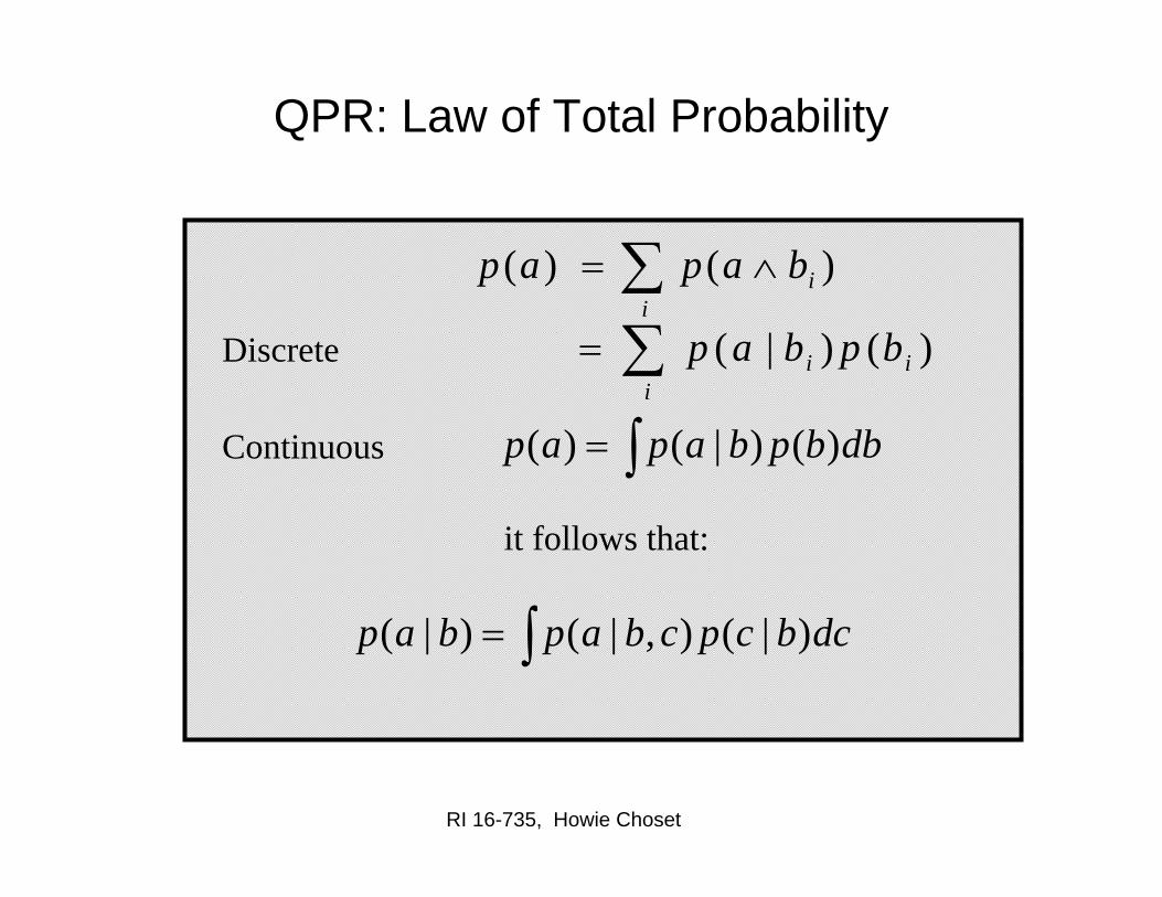
QPR: Law of Total Probability
∑ ∧=i
ibapap )()(
)()|( ii
i bpbap∑=Discrete
∫= dbbpbapap )()|()(Continuous
it follows that:
∫= dcbcpcbapbap )|(),|()|(
RI 16-735, Howie Choset
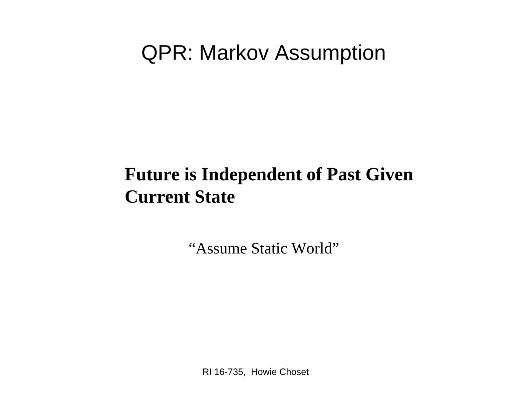
QPR: Markov Assumption
Future is Independent of Past Given Current State
“Assume Static World”

RI 16-735, Howie Choset
The Problem
• What is the world around me (mapping)– sense from various positions– integrate measurements to produce map– assumes perfect knowledge of position
• Where am I in the world (localization)– sense– relate sensor readings to a world model– compute location relative to model– assumes a perfect world model
• Together, these are SLAM (Simultaneous Localization and Mapping)
RI 16-735, Howie Choset
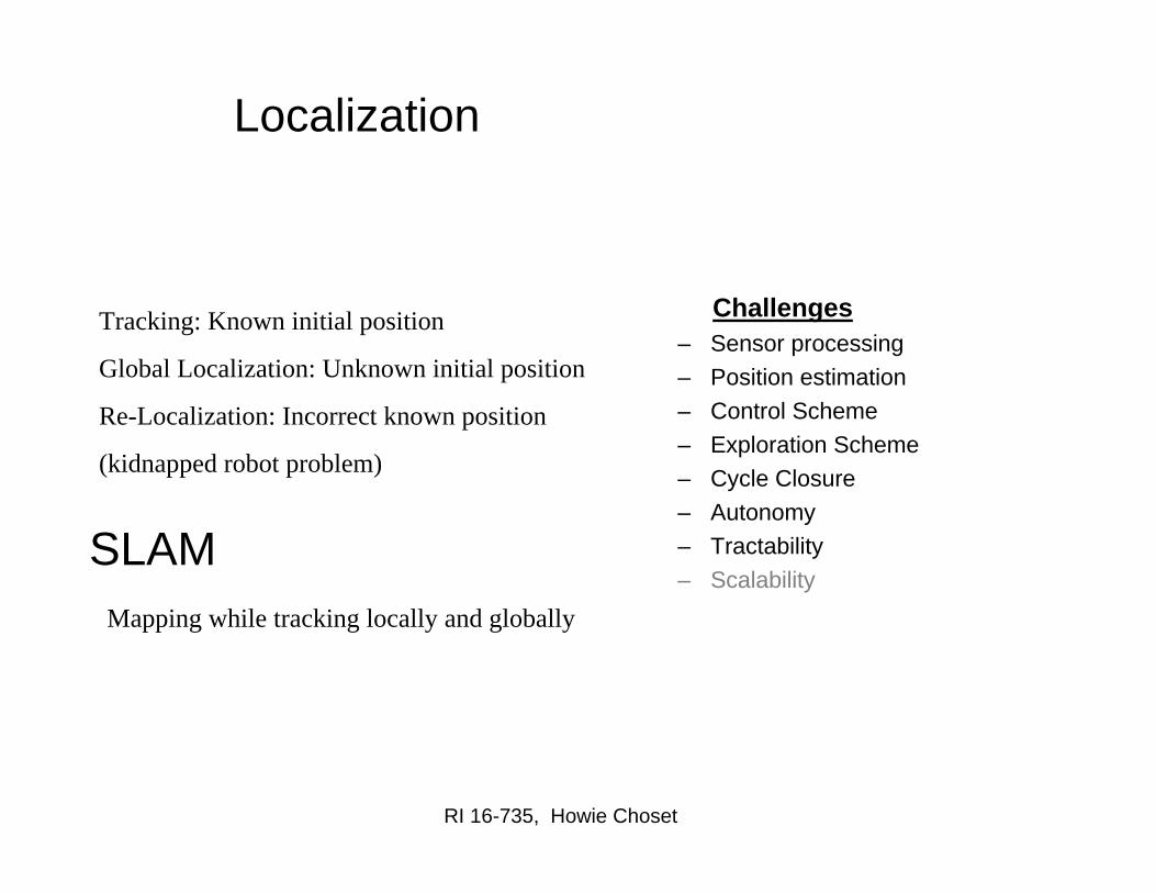
Localization
Tracking: Known initial position
Global Localization: Unknown initial position
Re-Localization: Incorrect known position
(kidnapped robot problem)
Challenges– Sensor processing– Position estimation– Control Scheme– Exploration Scheme– Cycle Closure– Autonomy– Tractability– Scalability
SLAMMapping while tracking locally and globally

RI 16-735, Howie Choset
Representations for Robot Localization
Discrete approaches (’95)• Topological representation (’95)
• uncertainty handling (POMDPs)• occas. global localization, recovery
• Grid-based, metric representation (’96)• global localization, recovery
Multi-hypothesis (’00)• multiple Kalman filters• global localization, recovery
Particle filters (’99)• sample-based representation• global localization, recovery
Kalman filters (late-80s?)• Gaussians• approximately linear models• position tracking
AI
Robotics

RI 16-735, Howie Choset
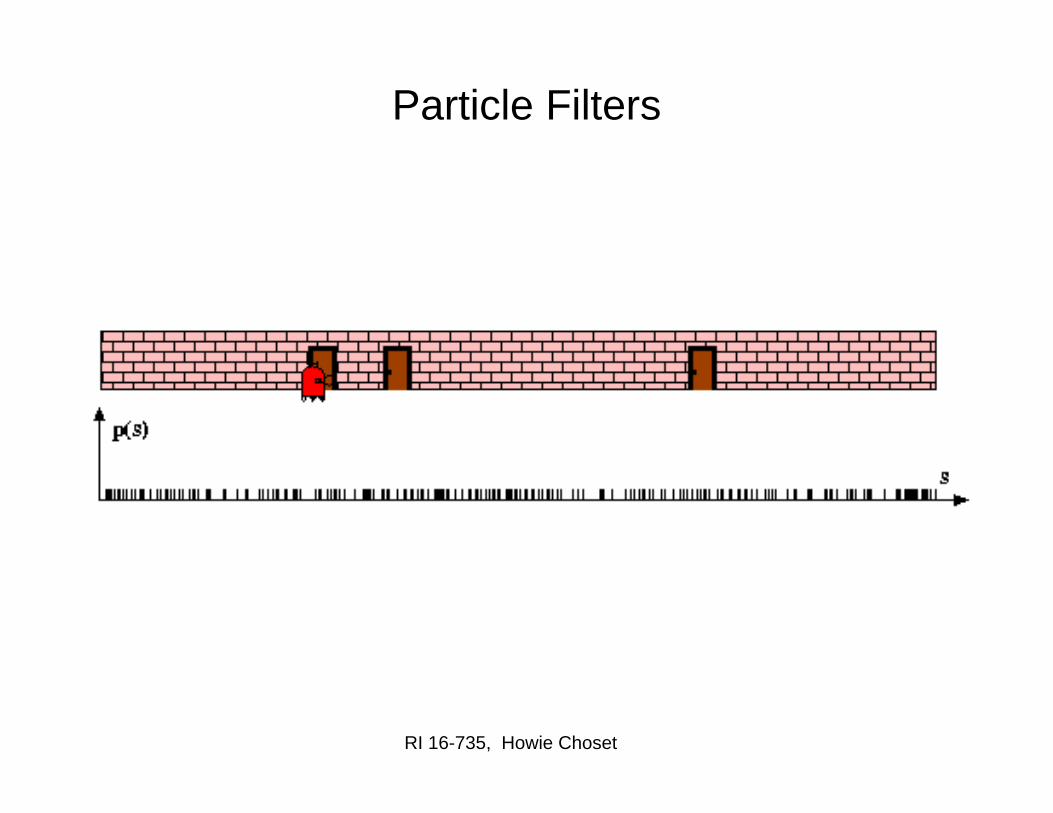
The Basic Idea
Robot can be anywhere
Robot senses a door
Robot moves on(note, not unimodal)
Robot senses another door(note, high likelihood, but multimodal)
[Simmons/Koenig 95][Kaelbling et al 96][Burgard et al 96]

RI 16-735, Howie Choset
Notes
• Perfect Sensing– No false positives/neg.– No error
• Data association

RI 16-735, Howie Choset
Notation for Localization
• At every step k
• Probability over all configurations
• Given– Sensor readings y from 1 to k– Control inputs u from 0 to k-1– Interleaved:
The posterior
Velocities, force, odometry, something more complicatedMap m (should be in condition statements too)

RI 16-735, Howie Choset
Predict and Update, combined
posterior
prior
Sensor model: robot perceives y(k) given a map and that it is at x(k)
Motion model: commanded motion moved from robot x(k-1) to x(k)
Issues
Realization of sensor and motion models
Representations of distributions
Features
Generalizes beyond Gaussians
Recursive Nature
RI 16-735, Howie Choset
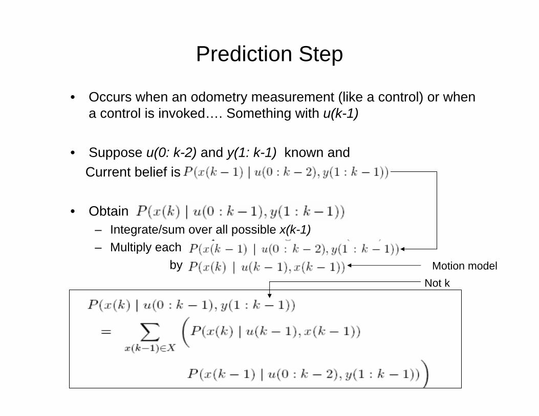
Prediction Step
• Occurs when an odometry measurement (like a control) or when a control is invoked…. Something with u(k-1)
• Suppose u(0: k-2) and y(1: k-1) known andCurrent belief is
• Obtain – Integrate/sum over all possible x(k-1)– Multiply each
by Motion modelNot k

RI 16-735, Howie Choset
Update Step
• Whenever a sensory experience occurs… something with y(k)
• Suppose is knownand we just had sensor y(k)
• For each state x(k)
Multiply by & ηSensor model
Normalization constant: make it all sum to one

RI 16-735, Howie Choset
That pesky normalization factor
• Bayes rule gives us
• This is hard to compute:– What is the dependency of y(k) on previous controls and sensor
readings without knowing your position or map of the world?
• Total probability saves the day
• We know these terms

RI 16-735, Howie Choset
Summary

RI 16-735, Howie Choset
Issues to be resolved
• Initial distribution P(0)– Gaussian if you have a good idea– Uniform if you have no idea– Whatever you want if you have some idea
• How to represent distributions: prior & posterior, sensor & motion models
• How to compute conditional probabilities
• Where does this all come from? (we will do that first)
RI 16-735, Howie Choset
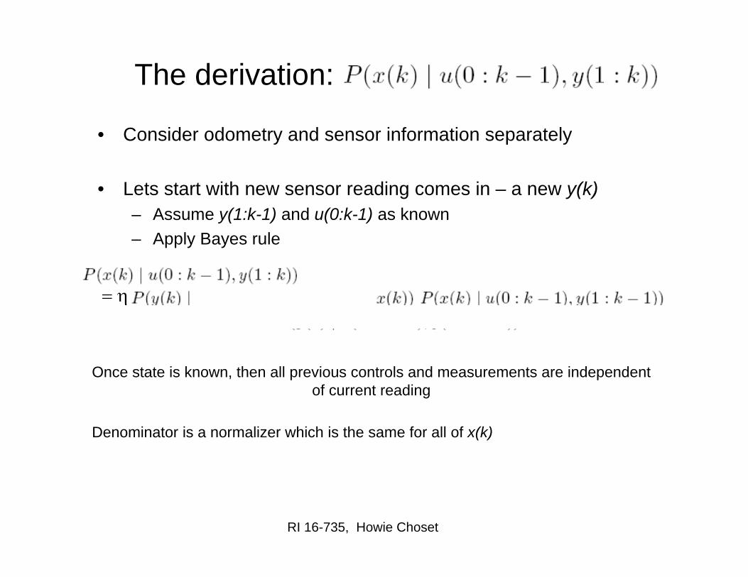
The derivation:
• Consider odometry and sensor information separately
• Lets start with new sensor reading comes in – a new y(k)– Assume y(1:k-1) and u(0:k-1) as known– Apply Bayes rule
Once state is known, then all previous controls and measurements are independent of current reading
Denominator is a normalizer which is the same for all of x(k)
= η

RI 16-735, Howie Choset
Incorporate motions
• We have
• Use law of total probability on right-most term
assume that x(k) is independent of sensor readings y(1:k-1) and controls u(1:k-2)that got the robot to state x(k-1) given we know the robot is at state x(k-1)
assume controls at k-1 take robot from x(k-1) to x(k), which we don’t know x(k) x(k-1) is independent of u(k-1)

RI 16-735, Howie Choset
Incorporate motions
• We have
RI 16-735, Howie Choset
Representations of Distributions
• Kalman Filters
• Discrete Approximations
• Particle Filters

RI 16-735, Howie Choset
Extended Kalman Filters
as a Gaussian
The GoodComputationally efficientEasy to implement
The BadLinear updatesUnimodal
RI 16-735, Howie Choset
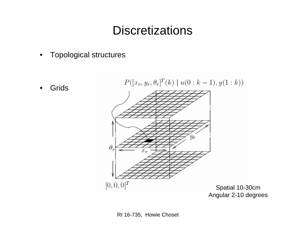
Discretizations
• Topological structures
• Grids
Spatial 10-30cmAngular 2-10 degrees

RI 16-735, Howie Choset
Algorithm to Update Posterior P(x)
k loops
Start with u(0: k-1) and y(1:k)
Integrate u(i-1) and y(i-1) in each loop
Incorporate motion u(i-1) with motionmodel
Sensor modelNormalization Constant
Bypass with convolution details we will skip

RI 16-735, Howie Choset
Convolution Mumbo Jumbo
• To efficiently update the belief upon robot motions, one typically assumes a bounded Gaussian model for the motion uncertainty.
• This reduces the update cost from O(n2) to O(n), where n is the number of states.
• The update can also be realized by shifting the data in the grid according to the measured motion.
• In a second step, the grid is then convolved using a separable Gaussian Kernel.
• Two-dimensional example:
1/4
1/4
1/2 1/4 1/2 1/4+≅
1/16
1/16
1/8
1/8
1/8
1/4
1/16
1/16
1/8
• Fewer arithmetic operations
• Easier to implement

RI 16-735, Howie Choset
Probabilistic Action model
40m 80m.
Darker area has higher probability.
xk-1 xk-1
uk-1
uk-1
p(x(k)|u(k-1),x(k-1))
Continuous probability density Bel(st) after moving
Thrun et. al.

RI 16-735, Howie Choset
Probabilistic Sensor Model
Probabilistic sensor model for laser range finders
y
P(y
|x)

RI 16-735, Howie Choset
One of Wolfram et al’s Experiments
5 scans 18 scans 24 scans
A, after 5 scans; B, after 18 scans, C, after 24 scans
Known map
RI 16-735, Howie Choset
What do you do with this info?• Mean, continuous but may not be meaningful
• Mode, max operator, not continuous but corresponds to a robot position
• Medians of x and y, may not correspond to a robot position too but robust to outliers

RI 16-735, Howie Choset
Represent belief by random samples
Estimation of non-Gaussian, nonlinear processes
Monte Carlo filter, Survival of the fittest, Condensation, Bootstrap filter, Particle filter
Filtering: [Rubin, 88], [Gordon et al., 93], [Kitagawa 96]
Computer vision: [Isard and Blake 96, 98]
Dynamic Bayesian Networks: [Kanazawa et al., 95]d
Particle Filters

RI 16-735, Howie Choset
Basic Idea
• Maintain a set of N samples of states, x, and weights, w, in a set called M.
• When a new measurement, y(k) comes in, the weight of particle (x,w) is computed as p(y(k)|x) – observation given a state
• Resample N samples (with replacement) from M according to weights w

RI 16-735, Howie Choset
draw xit−1 from Bel(xt−1)
draw xit from p(xt | xi
t−1,ut−1)
Importance factor for xit:
)|()(),|(
)(),|()|(ondistributi proposal
ondistributitarget
111
111
tt
tttt
tttttt
it
xypxBeluxxp
xBeluxxpxyp
w
∝
=
=
−−−
−−−η
1111 )(),|()|()( −−−−∫= tttttttt dxxBeluxxpxypxBel η
Particle Filter Algorithmand Recursive Localization
RI 16-735, Howie Choset
Particle Filters

RI 16-735, Howie Choset
)|()(
)()|()()|()(
xypxBel
xBelxypw
xBelxypxBel
αα
α
=←
←
−
−
−
Sensor Information: Importance Sampling

RI 16-735, Howie Choset
∫←− 'd)'()'|()( , xxBelxuxpxBel
Robot Motion

RI 16-735, Howie Choset
)|()(
)()|()()|()(
xypxBel
xBelxypw
xBelxypxBel
αα
α
=←
←
−
−
−
Sensor Information: Importance Sampling

RI 16-735, Howie Choset
Robot Motion
∫←− 'd)'()'|()( , xxBelxuxpxBel

RI 16-735, Howie Choset
Start
Motion Model Reminder
Or what if robot keeps moving and there are no observations
RI 16-735, Howie Choset
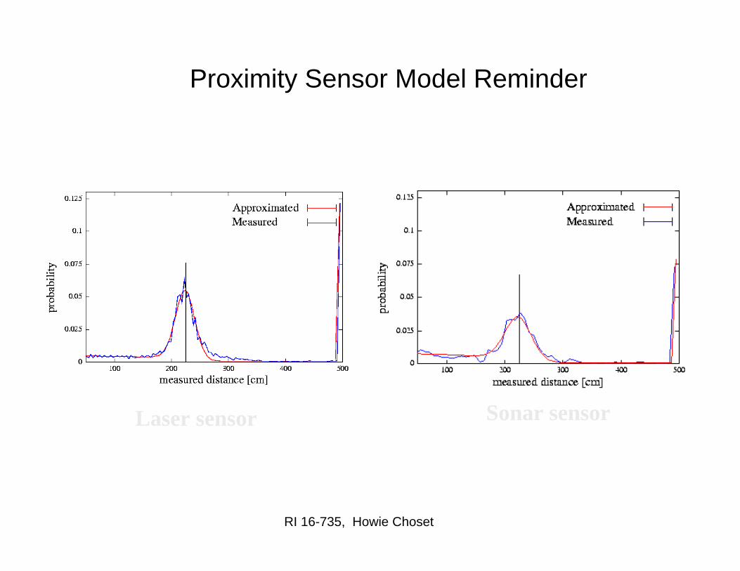
Proximity Sensor Model Reminder
Laser sensor Sonar sensor
RI 16-735, Howie Choset
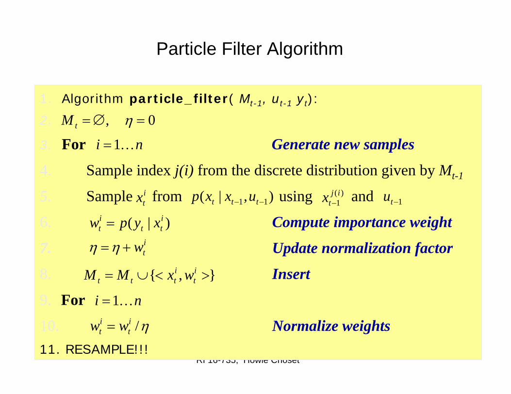
1. Algorithm particle_filter( Mt-1, ut-1 yt):
2.
3. For Generate new samples
4. Sample index j(i) from the discrete distribution given by Mt-1
5. Sample from using and
6. Compute importance weight
7. Update normalization factor
8. Insert
9. For
10. Normalize weights11. RESAMPLE!!!
Particle Filter Algorithm
0, =∅= ηtM
ni K1=
},{ ><∪= it
ittt wxMM
itw+=ηη
itx ),|( 11 −− ttt uxxp )(
1ij
tx − 1−tu
)|( itt
it xypw =
ni K1=
η/it
it ww =

RI 16-735, Howie Choset
Resampling
• Given: Set M of weighted samples.
• Wanted : Random sample, where the probability of drawing xi is given by wi.
• Typically done N times with replacement to generate new sample set M’.

RI 16-735, Howie Choset
1. Algorithm systematic_resampling(M,n):
2.3. For Generate cdf4.5. Initialize threshold
6. For Draw samples …7. While ( ) Skip until next threshold reached8.9. Insert10. Increment threshold
11. Return M’
Resampling Algorithm
11,' wcM =∅=
ni K2=i
ii wcc += −1
1],,0]~ 11 =− inUu
nj K1=
11
−+ += nuu jj
ij cu >
{ }><∪= −1,'' nxMM i
1+= ii

RI 16-735, Howie Choset
w2
w3
w1wn
Wn-1
Resampling, an analogy Wolfram likes
w2
w3
w1wn
Wn-1
• Roulette wheel
• Binary search, n log n
• Stochastic universal sampling
• Systematic resampling
• Linear time complexity
• Easy to implement, low variance

RI 16-735, Howie Choset
Initial Distribution
RI 16-735, Howie Choset
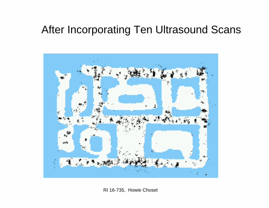
After Incorporating Ten Ultrasound Scans

RI 16-735, Howie Choset
After Incorporating 65 Ultrasound Scans

RI 16-735, Howie Choset
Limitations
• The approach described so far is able to – track the pose of a mobile robot and to– globally localize the robot.
• How can we deal with localization errors (i.e., the kidnapped robot problem)?
RI 16-735, Howie Choset
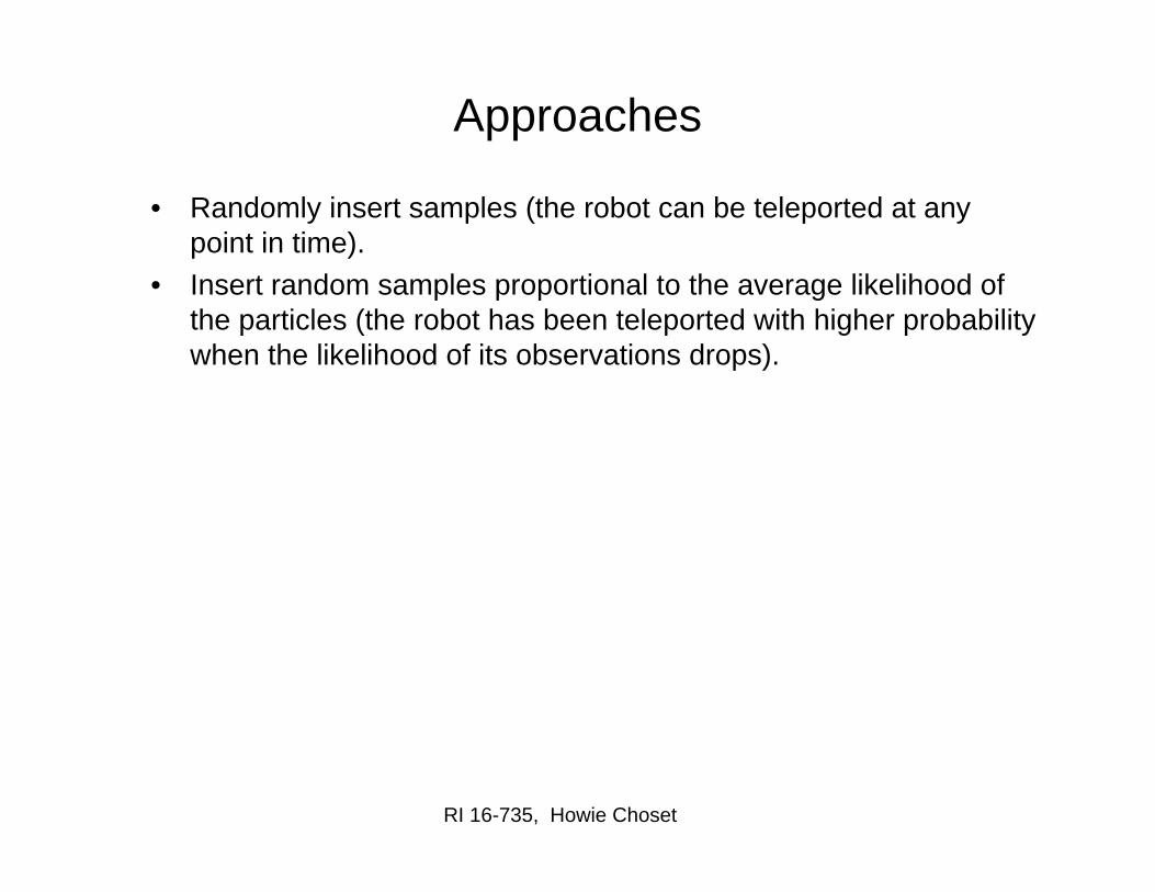
Approaches
• Randomly insert samples (the robot can be teleported at any point in time).
• Insert random samples proportional to the average likelihood of the particles (the robot has been teleported with higher probability when the likelihood of its observations drops).
RI 16-735, Howie Choset
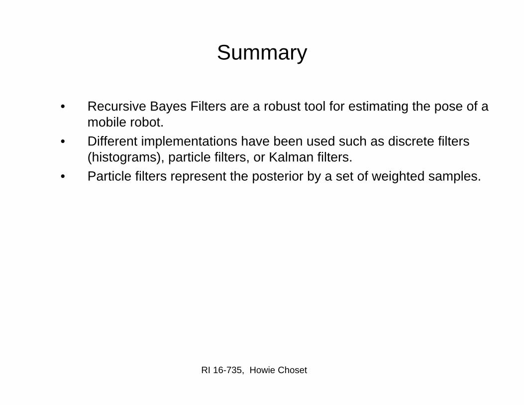
Summary
• Recursive Bayes Filters are a robust tool for estimating the pose of a mobile robot.
• Different implementations have been used such as discrete filters (histograms), particle filters, or Kalman filters.
• Particle filters represent the posterior by a set of weighted samples.

RI 16-735, Howie Choset
Change gears to

RI 16-735, Howie Choset
Occupancy Grids [Elfes]
• In the mid 80’s Elfes starting implementing cheap ultrasonic transducers on an autonomous robot
• Because of intrinsic limitations in any sonar, it is important to compose a coherent world-model using information gained from multiple reading

RI 16-735, Howie Choset
Occupancy Grids Defined
• The grid stores the probability that Ci = cell(x,y) is occupied O(Ci) = P[s(Ci) = OCC](Ci)
• Phases of Creating a Grid:– Collect reading generating O(Ci)– Update Occ. Grid creating a map– Match and Combine maps from multiple
locationsx
y
Ci
Original notation
Cell is occupied Given sensor observations Given robot locations
Binary variable
RI 16-735, Howie Choset
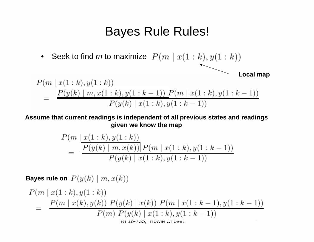
Bayes Rule Rules!
• Seek to find m to maximize
Assume that current readings is independent of all previous states and readings given we know the map
Bayes rule on
Local map
RI 16-735, Howie Choset
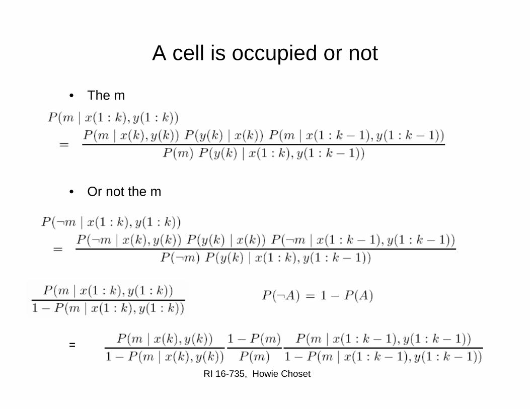
• The m
• Or not the m
A cell is occupied or not
=
RI 16-735, Howie Choset
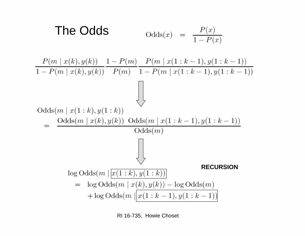
The Odds
RECURSION

RI 16-735, Howie Choset
Recover Probability
Given a sequence of measurements y(1:k), known positions x(1:k), and an initial distribution P0(m)
Determine
THE PRIOR

RI 16-735, Howie Choset
Actual Computation of
• Big Assumption: All Cells are Independent
• Now, we can update just a cell
Depends on current cell, distance to cell and angle to central axis
The prior
Local map

RI 16-735, Howie Choset
More details on s
Deviation from occupancy probability from the prior given a reading and angle
Else if’s
RI 16-735, Howie Choset
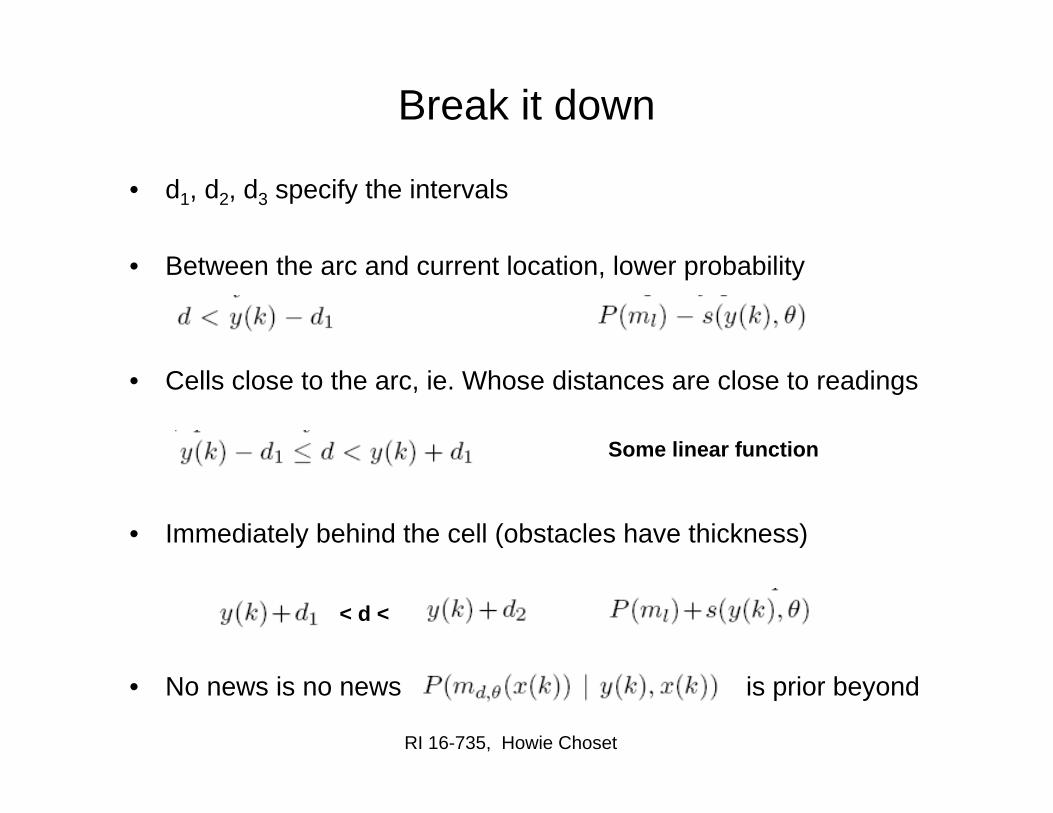
Break it down
• d1, d2, d3 specify the intervals
• Between the arc and current location, lower probability
• Cells close to the arc, ie. Whose distances are close to readings
• Immediately behind the cell (obstacles have thickness)
• No news is no news is prior beyond
Some linear function
< d <

RI 16-735, Howie Choset
Example
y(k) = 2m, angle = 0, s(2m,0) = .16

RI 16-735, Howie Choset
Example
y(k) = 2m y(k) = 2.5m

RI 16-735, Howie Choset
A Wolfram Mapping Experimentwith a B21r with 24 sonars
18 scans, note each scan looks a bit uncertain but result starts to look like parallel walls

RI 16-735, Howie Choset
Are we independent?
• Is this a bad assumption?
RI 16-735, Howie Choset
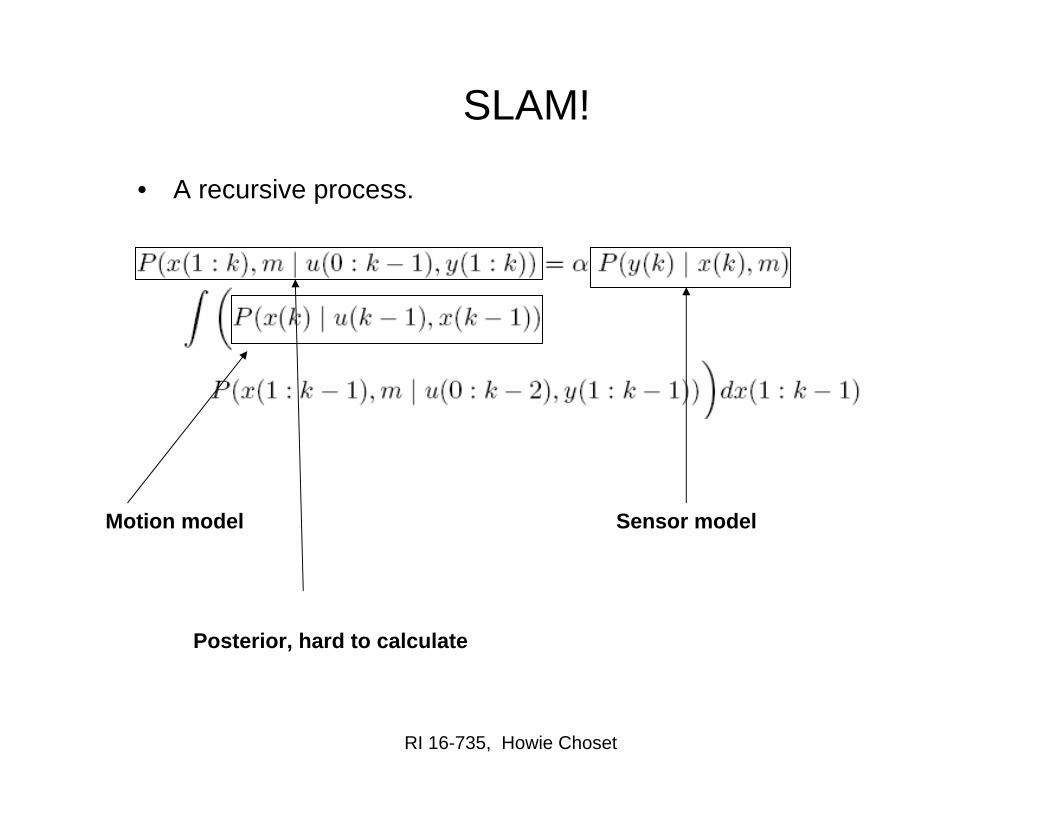
SLAM!
• A recursive process.
Motion model Sensor model
Posterior, hard to calculate

RI 16-735, Howie Choset
“Scan Matching”
At time the robot is given
1. An estimate of state
2. A map estimate
The robot then moves and takes measurement y(k)
And robot chooses state estimate which maximizes
And then the map is updated with the new sensor reading

RI 16-735, Howie Choset
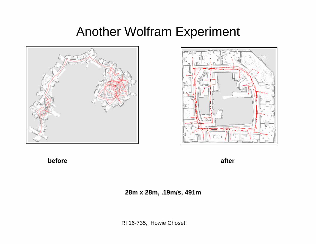
Another Wolfram Experiment
28m x 28m, .19m/s, 491m
after
RI 16-735, Howie Choset
Another Wolfram Experiment
28m x 28m, .19m/s, 491m
before after

RI 16-735, Howie Choset
Tech Museum, San Jose
CAD map occupancy grid map

RI 16-735, Howie Choset
Issues
• Greedy maximization step (unimodal)
• Computational burden (post-processing)
• Inconsistency (closing the loop, global map?)
Solutions [still maintain one map, but update at loop closing]• Grid-based technique (Konolodige et. al)• Particle Filtering (Thrun et. al., Murphy et. al.)• Topological/Hybrid approaches (Kuipers et. al, Leonard et al,
Choset et a.)

RI 16-735, Howie Choset
Probabilistic SLAMRao-Blackwell Particle Filtering
If we know the map, then it is a localization problemIf we know the landmarks, then it is a mapping problem
Some intuition: if we know x(1:k) (not x(0)), then we know the “relative map” butNot its global coordinates
The promise: once path (x(1:k)) is known, then map can be determined analytically
Find the path, then find the map

RI 16-735, Howie Choset
Mapping with Rao-Blackwellized Particle Filters
• Observation: Given the true trajectory of the robot, all measurements are independent.
• Idea:– Use a particle filter to represent potential trajectories of the robot
(multiple hypotheses). Each particle is a path (maintain posterior of paths)
– For each particle we can compute the map of the environment (mapping with known poses).
– Each particle survives with a probability that is proportional to the likelihood of the observation given that particle and its map.
[Murphy et al., 99]

RI 16-735, Howie Choset
RBPF with Grid Maps
map of particle 1 map of particle 3
map of particle 2
3 particles

RI 16-735, Howie Choset
Some derivation
P(A,B) = P(A|B)P(B)
given
We can compute Use particle filtering
Computing prob map (local map) given trajectory for each particle

RI 16-735, Howie Choset
Methodology• M be a set of particles where each particle starts at [0,0,0]T
• Let h(j)(1:k) be the jth path or particle
• Once the path is known, we can compute most likely map
• Once a new u(i-1) is received (we move), do same thing as in localization, i.e., sample from
– Note, really sampling from– Ignore the map for efficiency purposes, so drop the m
• Get our y(k)’s to determine weights, and away we go (use same sensor model as in localization)
Hands start waving….. Just a threshold here
Not an issue, but in book

RI 16-735, Howie Choset
Rao-Blackwell Particle Filtering
RI 16-735, Howie Choset
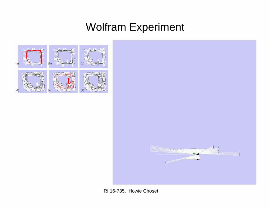
Wolfram Experiment

RI 16-735, Howie Choset
Most Recent Implementations
15 particles
four times faster than real-timeP4, 2.8GHz
5cm resolution during scan matching
1cm resolution in final map
Courtesy by Giorgio Grisetti & Cyrill Stachniss

RI 16-735, Howie Choset
Maps, space vs. time
Maintain a map for each particle
OR
Compute the map each time from scratch
Subject of researchMontermerlou and Thrun look for tree-like structures that capture commonality among particles.
Hahnel, Burgard, and Thrun use recent map and subsamplesensory experiences

RI 16-735, Howie Choset
How many particles?
• What does one mean?
• What does an infinite number mean?