


Languages
Pages
Legal


BACHELOR’S DEGREE ENERGY ENGINEERING
DESIGN OF A TEST RIG FOR PRESSURE-TIME BASED DISCHARGE
MEASUREMENT
Author: Joan Mateu Chiquin Font
Supervisor: Michel Cervantes
Luleå, Sweden 2020

1
ABSTRACT This thesis deals with the design and dimensioning of a water hammer test rig at the mechanical
engineering department of Lulea Tekniska Universitet. The system allows the study and further
development of the discharge measurement pressure-time method, often known as Gibson method,
with a variable cross-section pipe.
A theoretical study on water hammer transients and Gibson method constitutes a major part of this
document. A detailed explanation of its causes and consequences was carried out, alongside with a
literature review and previous investigations.
On the other hand, diverse calculations have been done to predict the behavior of the water hammer
transient and calculate the maximum pressure and working flow rate of the system. Along with a
numerical simulation of this phenomena, these calculations have played a major role in the selection
of the components. A variety of retailers were contacted to obtain a complete budget for the system,
not without contemplating beforehand the different options and possible working modes of the test
rig. Furthermore, in collaboration with other students, an automatic electrical system was designed
for the fast valve closure with variable closing times.
Due to the current global COVID-19 pandemic and the ongoing water proofing of the floor at the
laboratory where the test rig is thought to be placed, it has not been possible to execute the building
phase of this project. Nevertheless, the system has been fully designed and only the experimental
results are pending. The test rig’s building phase and experimental data collection will be
appropriately carried out when the laboratory’s conditions allow it.

2
Contents Nomenclature ........................................................................................................................... 4
1. Introduction .......................................................................................................................... 5
2. Objective ............................................................................................................................... 5
3. Theoretical background .......................................................................................................... 6
3.1 Water hammer ........................................................................................................................... 6
3.2 Discharge measurement methods .............................................................................................. 9
3.2.1 Pressure-area based flow measurement ............................................................................. 9
3.2.2 Pressure-time based flow measurement .......................................................................... 10
3.3 Literature review for Gibson method testing ........................................................................... 11
4. Mathematical model & numerical simulation ....................................................................... 13
4.1 Method of characteristics ......................................................................................................... 13
4.1 Simulation results ..................................................................................................................... 13
5. Test rig design ...................................................................................................................... 15
5.1 General system design .............................................................................................................. 15
5.1.1 Tank’s flow control ............................................................................................................ 16
5.2 Pipe thickness and loss calculation ........................................................................................... 18
5.3 Total head calculation and pumping system design ................................................................. 19
5.4 Valve closure system ................................................................................................................ 20
5.4.1 Electromechanic closing mechanism ................................................................................. 21
5.5 Budget ....................................................................................................................................... 22
6. Building phase ..................................................................................................................... 22
6.1 Task list ..................................................................................................................................... 22
6.2 Planning .................................................................................................................................... 24
7. Risk analysis ........................................................................................................................ 25
8. Conclusions ......................................................................................................................... 26
References .............................................................................................................................. 27
Appendix................................................................................................................................. 29
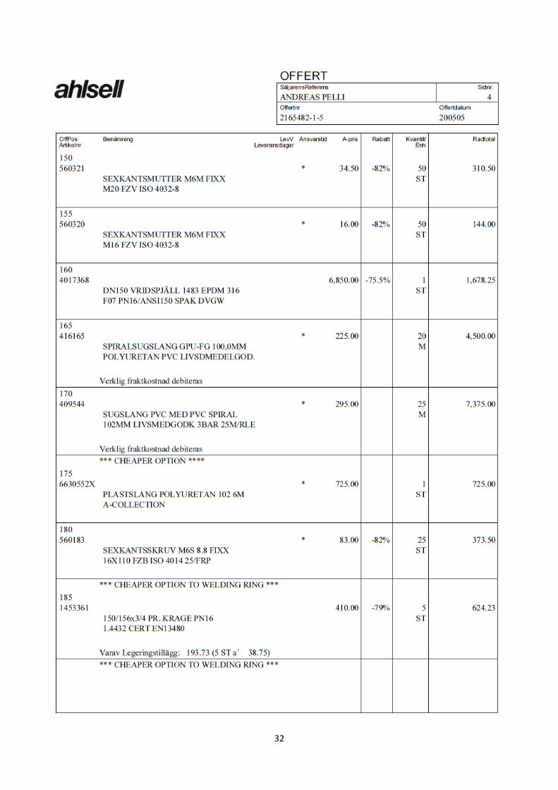
A. Retailers’ offers .......................................................................................................................... 29
A.1 Ahlsell: components ............................................................................................................. 29
A.2. Ahlsell: Pump ....................................................................................................................... 34
A.3. Ventim: electromagnetic flow meter .................................................................................. 36
A.4. Scandia Pumps: Level Sensor .............................................................................................. 37

3
A.5. ABB: Variable Frequency Drive ............................................................................................ 38
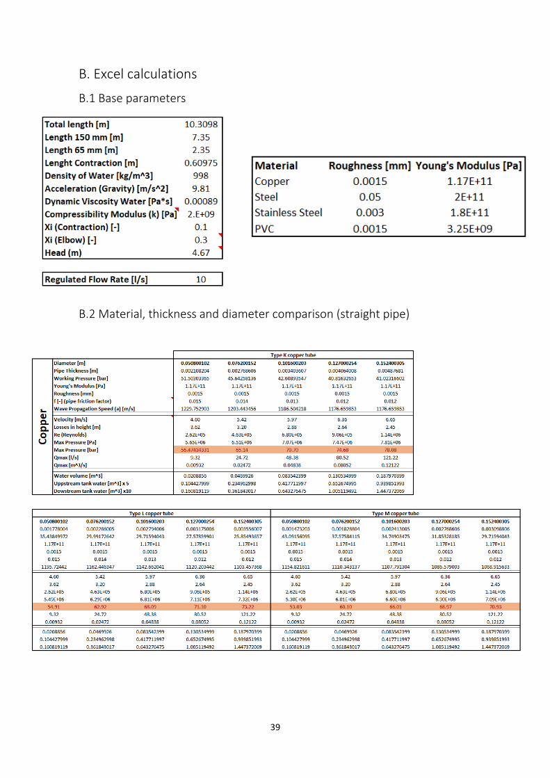
B. Excel calculations ........................................................................................................................ 39
B.1 Base parameters ................................................................................................................... 39
B.2 Material, thickness and diameter comparison (straight pipe) ............................................. 39
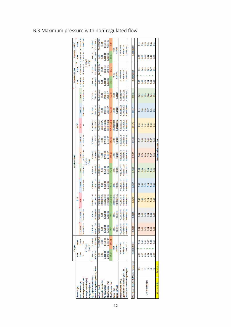
B.3 Maximum pressure with non-regulated flow ....................................................................... 42
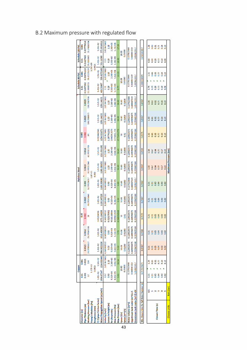
B.2 Maximum pressure with regulated flow .............................................................................. 43
C. Budget ......................................................................................................................................... 44
D. Pertt Diagram ............................................................................................................................. 45
E. 2D Planes .................................................................................................................................... 46
E.1 Plane 1: Detailed test rig ....................................................................................................... 46
E.2 Plane 2: Additional components ........................................................................................... 48

4
Nomenclature Greek Characters
μ – Dynamic Viscosity [Pas]
ε – Young’s Modulus of Elasticity [Pa]
α – Coriolis coefficient (kinetic energy correction coefficient)
ρ – Density [kg/m3]
Roman Characters
t - time [s]
V - Volume [m3]
A – Area [m2]
a – Wave Speed [m/s]
c – Initial velocity of the fluid [m/s]
m – Mass [kg]
Q – Volumetric flow rate [m3/s]
P – Pressure [Pa]
ΔPf – Pressure losses due to friction [Pa]
ΔPd – Dynamic pressure difference [Pa]
p – Momentum [kgm/s]
e – Thickness of the pipe [m]
k – Compressibility modulus of water [Pa]
D – Diameter of the pipe [m]
L – Length of the pipe [m]
Tr – Return time of the pressure wave [s]
TL – Closure time of the valve [s]
f – Friction factor [ ]
T – Period of the water hammer wave [s]
Z – Height [m]
Hf – Friction Losses [ ]
U – Voltage [V]
Re – Reynold’s Number
5
1. Introduction Piping systems are widely used in many areas of modern industry and engineering. In a day-to-day
usage their existence seems natural, although there is a lot to understand about how they operate
for proper functioning. Their complexity has raised due to the variety of applications they have; from
small pipes transporting water for domestic purposes to large networks of piping for the production
of electricity in big nuclear or hydropower plants, with extreme temperatures and pressures and
more complex fluids like molten salts or oil.
Different phenomena occur in these systems. During the realization of this project, the water
hammer effect is deeply studied and applied. It consists on a pressure wave that propagates through
the pipe as a consequence of a sudden change in momentum of the flow. In modern engineering,
this event is not overlooked; if a system is not designed properly, the pressure spikes consequence
of the water hammer can severely damage installations and personnel.
In Sweden, during 2017, nuclear power and hydropower represented more than 75% of the
generated energy [1] and together constituted a total of 128 TWh of generated energy. Both major
electricity generation agents have highly complex piping systems that might suffer the effects of
water hammer transient pressure if not handled properly. The reliability and security of the nuclear
systems are essential; they could obtain a great benefit from the usage of a more precise and reliable
discharge measurement method. In the other hand, hydropower plants constantly deal with load
rejection and therefore, sudden changes in momentum in order to balance the energy generation.
The measurement of the efficiency in these systems is highly dependent on the flow rate data. This
property, also known as discharge, is defined as the volume of liquid flowing through a specified area
during a certain time. To determine the hydraulic performance of big pumps and turbines, for
example, the measurement of the discharge is crucial and presents a high level of difficulty in
comparison to other properties of a fluid through a pipe (i.e. Power or head).
There are several methods known for its measurement and, naturally, each one of them presents
certain conditions that limit their applications. The most used ones are the velocity-area method,
pressure-time method (Gibson method), ultrasonic method, tracer method and electromagnetic
method, see 3. Literature Study. In the present project, the methods that have the most relevance
are the Gibson and electromagnetic methods, as the test rig is designed to test development of the
Gibson method and will use the electromagnetic flow sensor as reference.
2. Objective The objective of this project is to design and build a test rig for measuring the water flow rate running
through a pipe of variable cross-section using the pressure-time method , comparing the results with
the measurements obtained from electromagnetic flow sensors.
A secondary aim of the project is to study the maximum pressure in a water hammer pressure surge,
in function of the closure time (from instantaneous to larger time) on the test rig.

6
3. Theoretical background
3.1 Water hammer When a valve is closed rapidly in a pipe network, the transformation of momentum into pressure
gives rise to a hydraulic transient, a pressure spike, known as a water hammer. This phenomenon
travels as a wave along the pipe and goes back and forth until the friction losses dissipate its effect.
As represented in Figure 1, when there’s a given flow in a pipe (t=0) and a sudden change in
momentum occurs, like a valve closure, there is a pressure rise that propagates through the pipe
(0<t<To) to even out the pressure difference until it reaches the reservoir (t=To). At this point, the
pressure in the pipe is higher than the pressure in the reservoir, which causes the flow to move
towards the reservoir (To<t<2To), creating a low-pressure area when the wave reaches the valve
again (t=2To). This low-pressure wave travels back to the reservoir (t=3To), and the flow starts to
flow towards the pipe, creating a high-pressure area in the valve (t=4To). This process repeats itself
until the wave is dissipated by friction losses.
The maximum pressure during this process can be mathematically formulated using the 2nd Newton’s
law, conservation of momentum (Eq. 1), which states that the change in momentum in a system is
equal to the forces exerted on the system by its surroundings. The mass conservation principle also
plays an important role to describe the behavior of the fluid (Eq. 2):
∑𝐹 =∂p
∂t (1)
∂m
∂t= 0 (2)
The mass conservation equation develops to the continuity equation:
∂(ρA)
∂t+∂(ρAV)
∂x= 0
(3)
(3)
And the momentum equation can be developed taking into account that the Force [N] for a given
flow in a pipe is equivalent to the change of pressure [N/ m2] times the area of the pipe [m2] (Eq. 5)
and that the right-hand side of Eq. 4 can be developed as presented in Eq. 6
F = m ∙∂c
∂t (4)
𝐹 = ∆P ∙ 𝐴 (5)
m ∙∂c
∂t= 𝑎 ∙ 𝐴 ∙ 𝜌 ∙ 𝑐 (6)
Consequently, Eq. 7 is obtained and simplified, obtaining the so-called Jukowski’s equation (after the
mathematician Nikolay Yegorovich Zhukovsky) , that describes the pressure rise due to water
hammer effect (see Eq. 8):
∆P ∙ 𝐴 = a ∙ 𝐴 ∙ 𝜌 ∙ 𝑐 (7)
∆P = a ∙ 𝜌 ∙ 𝑐 (8)

7
Figure 1: Water hammer wave [2]
Hooke’s Law can be used to describe the elasticity of water in a closed conduit, which is affected by
the elasticity of the conduit itself. Both are directly related to the water hammer wave propagation
speed as follows:
a = √1
𝜌 ∙ (1𝑘+
𝐷𝜀 ∙ 𝑒)
(9)
It is important to note that, in the instant when the valve begins its closure, the wave starts
propagating and will come back in a time Tr. If the valve is not fully closed by this then, the pressure
rise is not equal to the one described by Jukowski’s equation (Eq. 8). Hence:
𝑇𝑟 =2𝐿
𝑎 (10)
𝑇 =4𝐿
𝑎 (11)

8
When the valve is closed fast enough, the pressure wave follows the diagram of Figure 2. Otherwise,
the Jukowski’s pressure is not achieved and the pressure wave behaves as described in Figure 3.
Figure 2: Water hammer wave propagation with fast closure [3]
Figure 3: Water hammer wave propagation with slow closure [3]
Since the Jukowski’s equation doesn’t apply for the second case, as the pressure doesn’t reach the
maximum level, the closure time variable can be added to the formula as described in equation 12.
The water hammer pressure rise will consequently be maximum as long as the closure time follows
the behavior described in Eq. 13.
∆P = a ∙ 𝜌 ∙ 𝑐 ∙𝑇𝑟
𝑇𝐿 (12)
𝑇𝐿 ≤2𝐿
𝑎 (13)

9
3.2 Discharge measurement methods
3.2.1 Pressure-area based flow measurement Measuring the volumetric flow rate in a small pipe does not represent a problem in modern
engineering. Usually these systems are cheaper to handle, and the small dimensions allow the usage
of apparatus (like electromagnetic flow meters) that wouldn’t work for larger systems.
The usage of nozzles, venturi tubes or orifice plates is widely extended. These are pressure-based
flow meters and their working principle is based on the creation of a difference in pressure along the
tube by changing the diameter of the pipe and constricting the flow rate. Measuring the pressure
difference and applying the Bernoulli’s and continuity equations (Eq. 14 & 15), it is possible to
calculate the discharge reliably and accurately.
𝑃1 +ρ𝑐1
2
2+ ρg𝑧1 = 𝑃2 +
ρ𝑐22
2+ ρg𝑧2 + ℎ𝑓 (14)
𝐴1 ∙ 𝑐1 = 𝐴2 ∙ 𝑐2 = 𝑄 (15)
Figure 4: Pressure-based flow meters [4]
These allow the continuous measurement of the flow rate and are very common for small pipes.
However, they are not suitable for large diameter piping systems, of several meters in diameter. They
represent significant losses in friction and the large dimensions of power plants are an inconvenient
for the usage of these flow meters.
Unfortunately, the usage of these methods is not only unpractical but very difficult to implement in
hydroelectric power plants, where the diameter and dimensions of pipes and the rest of components
is particularly large. Accordingly, it is necessary to have alternative methods, such as electromagnetic
flow meters, pressure-time based measurements and others.
3.2.1.2 Electromagnetic flow measurement
Based on Faraday’s law of induction, an electromagnetic flow meter consists basically on two field
coils and two electrodes. The field coils generate a constant magnetic field over the cross-section of

10
the measuring tube; when there is a conductive fluid running through the pipe, e.g., water. The
magnetic field applies a force on the positively and negatively charged particles running through the
pipe, causing them to separate. An electrical voltage forms and is measured by the electrodes. This
voltage is directly related to the velocity of the fluid and its behavior can be mathematically described
as follows:
U = k ∙ B ∙ 𝑐 ∙ 𝐷 (16)
Where D represents the distance between the electrodes, usually the diameter of the pipe, and k is
a dimensionless constant to be determined from calibration.
Figure 5: Scheme of an electromagnetic flow meter [5]
One of the main advantages of this measurement method is the non-intrusion of the pipe, allowing
the flow to continue without any extra losses. It usually works with pipes with diameters of up to 2
meters [6]. There is no additional frictional loss or pressure drop from its usage. However, it can only
be used with an electrically conductive fluid.
3.2.2 Pressure-time based flow measurement A larger diameter system implies higher complexity of its components and higher cost of handling
them. Often, large diameter pipes are designed without considering the measurement systems and
stopping the flow through a large pipe in order to install them is highly costly.
The Gibson method, after Norman R. Gibson who introduced it in 1923, is a method for discharge
measurement. It is based on hydraulic transients, the change of momentum into pressure and the
water hammer phenomenon (see 3.1 Water hammer), in a pipeline to determine the flow rate.
Lately, it has been gaining interest due to its low costs thanks to the advances of computer and data
acquisition systems that allow easier and more accurate measurement [7].
When there is a change in momentum of a fluid flowing through a pipe, a pressure difference is
created and propagates as a wave. For the Gibson method, the fluid is commonly decelerated
because of a shut off-device such as a valve or the wicket vanes of a turbine. The consequential
pressure difference is measured between two cross sections of the penstock and recorded in a time

11
diagram (see figure 6). This data can be used to calculate the volumetric flow rate before the
momentum change through proper integration, usually within a period of 4 to 10 seconds [8].
Figure 6: Time-history of the pressure difference measured [9]
Mathematically the Gibson’s method can be developed describing the fluid through a pipe using the
one-dimensional unsteady flow energy equation:
𝛼1 ∙𝜌𝑄2
2𝐴12 + 𝑃1 + ρg𝑧1 = 𝛼2 ∙
𝜌𝑄2
2𝐴22 + 𝑃2 + ρg𝑧2 + ∆𝑃𝑓 + 𝜌 ∙
𝜕𝑄
𝜕𝑡∫
𝜕𝑥
𝐴(𝑥)
𝐿
0
(17)
Where the Coriolis coefficients range between 1.04 and 1.11 for fully developed turbulent flow in a
round pipe [10]. Stating the equivalences represented in Eq. 18-20:
∆P = (𝑃2 + ρg𝑧2) − (𝑃1 + ρg𝑧1) (18)
∆𝑃𝑑 = 𝜌𝑄2 ∙ (𝛼2
2𝐴22 −
𝛼1
2𝐴12) (19)
F = ∫𝜕𝑥
𝐴(𝑥)
𝐿
0
(20)
And finally, substituting the above notations in Eq. 15, it can be expressed in differential form (Eq.
21), and obtain the expression for the volumetric flow rate (Eq. 22) after integrating over the time
interval (t0-t1).
𝜌𝐹 ∙𝜕𝑄
𝜕𝑡= ∆P − ∆𝑃𝑑 − ∆𝑃𝑓 (21)
𝑄0 =1
𝜌𝐹∙ ∫ (∆P(t) + ∆𝑃𝑑(𝑡) + ∆𝑃𝑓(𝑡)) 𝑑𝑡 + 𝑄1
𝑡1
𝑡0
(22)
Where ΔPf and ΔPd are the pressure losses due to friction and dynamic pressure difference,
respectively.
3.3 Literature review for Gibson method testing The Gibson method, presented in its original version, has some limitations and conditions. One of
the main issues related to the method is the fact that the friction is considered steady, although this
factor is rarely steady, and this assumption is hardly correct in most of the cases. Nonetheless its
related added uncertainty is small and the measurement doesn’t differ more than 2% from the
reality[11].

12
Some other conditions for this method to work properly is the necessity of a distance greater than
10 meters between the pressure measuring points; the product of this length and the mean velocity
of the fluid before closure must be greater than 50 m2/s, as pointed by Dunca et al. [12] . These
limitations are related to the relative error of the estimation and measure, which increases when the
test section is reduced.
These reasons have encouraged the research and development of the pressure-time method by
different authors, leading to the decrease of its uncertainty. Johnson et al. [13] implemented an
unsteady friction factor that reduced the estimation error by a factor of 0.4%.
In the original Gibson method, the friction factor is assumed constant related to the initial flow rate
and the pressure history is integrated in an iterative loop, where the losses curve is determined. In
the research, the Gibson method is developed by using the Brunone friction model (Equation 23).
Instead of calculating the friction losses based on the initial flow, these factors are calculated at each
time step and node.
f = 𝑓𝑞 +𝑘𝐷
𝑉|𝑉|∙ (𝜕𝑉
𝜕𝑡− 𝑎 ∙
𝜕𝑉
𝜕𝑥) (23)
Where k is the Brunone friction coefficient, which can be calculated by trial and error or using the
Vardy’s coefficient (obtained based on the Reynold’s number) and 𝑓𝑞 is the quasi-steady friction
factor, described in the well-known Haaland equation for turbulent flow:
1
√𝑓𝑞= −1.8 ∙ log [(
𝜀/𝐷
3.7)1.11
+6.9
𝑅𝑒] (24)
Furthermore, other developments have been done in different studies. Adamkowski and Janicki [14]
implemented the usage of water hammer equations with the method of characteristics (MOC) and
the consideration of the pipe and liquid deformability via the calculation of the speed of sound (see
equation 9). Further advances were made by Dunca et al. [12] using the latter Adamkowski’s model
and applying an unsteady friction factor and the water hammer and wave speed equations. After
numerical and experimental analysis of the results, this research achieved the reduction of the
discharge estimation error by 0.6%.
Using the test rig under development along with numerical evaluation methods, further
development of the pressure-time method for pipe of variable cross-section will be possible.
The pipe geometry in the laboratory is not a straight pipe with a constant cross-section. It has a
contraction and an elbow (see 5.1 General system design). The presence of the contraction has a
direct relationship with one objectives of the project, the study and development of the Gibson
method with a variable cross-section pipe. On the other hand, the presence of an elbow in the test
rig represents a challenge, as noted by Adamkowski [8, p103]:
“Following the classical approach (version 1), the pressure-time method applicability is limited to
straight cylindrical pipelines with constant diameters. However, the IEC 60041 standard does not
exclude application of this method to more complex geometries, i.e. curved penstock (with an elbow).
It is obvious that a curved pipeline causes deformation of the uniform velocity field in its cross-
13
sections, which subsequently causes aggravation of the accuracy of the pressure-time method flow
rate measurement results”
Nonetheless, the influence of the elbow in the water hammer transient has already been studied by
Dalleli et al. [15] and it was observed that there’s no pressure reflection as long as the elbow is
immobile. However, if the elbow is not well restrained it can cause an increase of 33% of the
maximum pressure.
4. Mathematical model & numerical simulation
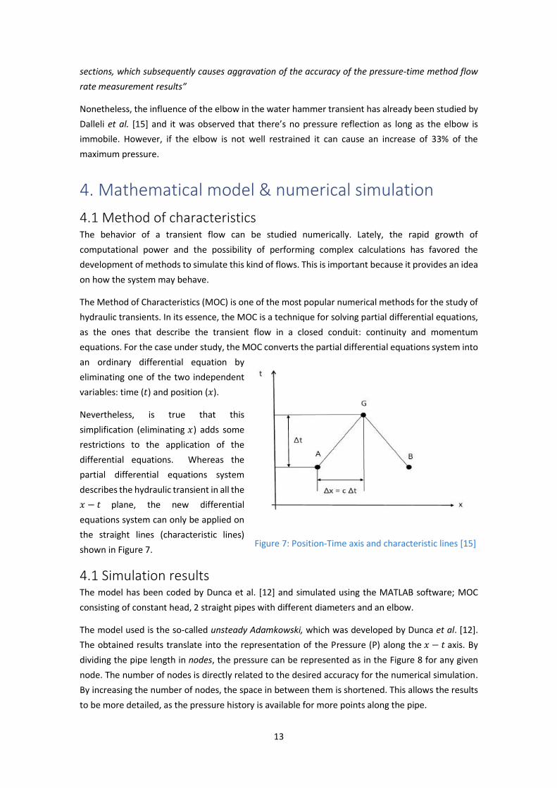
4.1 Method of characteristics The behavior of a transient flow can be studied numerically. Lately, the rapid growth of
computational power and the possibility of performing complex calculations has favored the
development of methods to simulate this kind of flows. This is important because it provides an idea
on how the system may behave.
The Method of Characteristics (MOC) is one of the most popular numerical methods for the study of
hydraulic transients. In its essence, the MOC is a technique for solving partial differential equations,
as the ones that describe the transient flow in a closed conduit: continuity and momentum
equations. For the case under study, the MOC converts the partial differential equations system into
an ordinary differential equation by
eliminating one of the two independent
variables: time (𝑡) and position (𝑥)..[16]
Nevertheless, is true that this
simplification (eliminating 𝑥) adds some
restrictions to the application of the
differential equations. Whereas the
partial differential equations system
describes the hydraulic transient in all the
𝑥 − 𝑡 plane, the new differential
equations system can only be applied on
the straight lines (characteristic lines)
shown in Figure 7.
4.1 Simulation results The model has been coded by Dunca et al. [12] and simulated using the MATLAB software; MOC
consisting of constant head, 2 straight pipes with different diameters and an elbow.
The model used is the so-called unsteady Adamkowski, which was developed by Dunca et al. [12].
The obtained results translate into the representation of the Pressure (P) along the 𝑥 − 𝑡 axis. By
dividing the pipe length in nodes, the pressure can be represented as in the Figure 8 for any given
node. The number of nodes is directly related to the desired accuracy for the numerical simulation.
By increasing the number of nodes, the space in between them is shortened. This allows the results
to be more detailed, as the pressure history is available for more points along the pipe.
Figure 7: Position-Time axis and characteristic lines [15]

14
Figure 8: Pressure history for the end node using MATLAB (Pressure-time)
By studying the length of the pipe, it is decided to use 19 nodes (including the beginning-end nodes).
The pressure history is available every 0.5 m along the full length of the pipe. Using the parameters
indicated in 5.1 General system design, the maximum pressure can be obtained for every node and
for different closure times (see Table 1), where Node 1 is the beginning of the 150 mm pipe starting
from the upstream tank and Node 19 is the end of the 65 mm pipe ending with the downstream
tank.
Table 1: Pressure in function of Node & Closure Time

15
5. Test rig design
5.1 General system design The main purpose of the system is to test the Gibson method in a geometry of variable cross-section,
recording the data of the pressure rise that occurs when interrupting the flow abruptly. Therefore,
the designed system consists on a couple of tanks (A & B) at different heights, in between which the
water flows in a closed circuit, as it can be seen in the scheme of Figures 9 & 10. The detailed
dimensions of the test rig are represented in the technical plans attached in Appendix E.1.
Figure 9: Test rig 3D model
Figure 10: Test rig 3D model

16
As illustrated, the system presents 2 elbows and a contraction. From the downstream tank (B), the
water is pumped back up (through pipe 2) with a higher flow rate than the one going downstream
through pipe 1.
From a general point of view, the test rig has the following dimensions & components:
• Pipe 1: Fully Stainless Steel, it is
formed by 7.35m of DN150x2 mm
pipe, the contraction and 2.35 m of
DN65x2mm pipe.
• Pipes 2&3: DN100 Flexible PVC pipes,
with a length of 10.3 m each.
• Tank A: 80x130x160 mm
• Tank B: 122.5x0.72.5x75 mm
• DN150 Manual valve: For pipe 1
• DN150-65 Contraction: to connect
both parts of pipe 1.
• 2xDN100 Manual valve: For pipes 2 &
3
• DN65 Fast closure valve: Closed by
an electrical motor, connected to a
gear system.
• DN65 Flowmeter: To measure the
flow.
• DN65 Butterfly valve: For flow
regulating purposes
• Safety valve: Set to 10 bar, pressure
at which the valve will open
Regarding the position of the valves and flowmeter in the DN65 part of pipe 1, it is important to
consider some distance in between these elements to avoid disturbances. From the DN150-65
contraction, a minimum distance of 10 diameters (0.65 m) and the fast-closure valve is considered.
In between the latter and the electromagnetic flowmeter, a minimum of 10 diameters. Finally, in
between the flowmeter and the flow-regulating butterfly valve, a minimum of 5 diameters. These
dimensions are schematized in the 2D plane available in Appendix E.2.
It is also important a smooth decrease in the diameter from pipe 1 to pipe 2. Taking into account that
the contractions provided by the supplier (view Appendix A.1) have a relatively large angle (9.46°), a
new contraction will be considered for the simulation and 3D models. The angle of the contraction
considered is 4°, with a final length of 609.75mm.
5.1.1 Tank’s flow control As a result of the higher flow rate in the inlet pipe compared to the outlet one, there will be an excess
water in the upstream tank (A). This tank is designed with inner separations, see in Figures 11 and
12. As the water comes in from pipe 2, the inner walls of the tank will allow the flow to go towards
the inlet of pipe 1 through check valves. Since not all the flow will go down pipe 1, there will be some
overflow towards the inlet of pipe 3, which is connected to the downstream tank (B). The purpose
of this system is to maintain a sustained water volume, keeping the testing conditions constant.

17
The inner walls, separating the inlet and outlet compartments, are designed to maintain a constant
water level (in reference to the tank’s floor) of 1.2 m for compartment 1.
The downstream tank includes an inner compartmentation similar to the one in the upstream tank,
with the same purpose, separating the inlet and outlet pipes. The dimensions for these inner
separations can be appreciated in Figures 13, 14 and with more detail in Appendix E.1.
At last, both tanks have been provided with a couple of DN25 drain valves, which facilitate the
process of emptying the tanks in case of need. These drain valves are located in compartments 1 and
2 for the tank A and in both compartments of tank B. Section 3 of the upstream tank already drains
the water downstream to the downstream tank, thus, it doesn’t need any drain valve.
Figure 12: Inner separations of
upstream tank
Figure 13: Downstream tank’s inner compartmentation Figure 14: Downstream tank’s top view
Figure 11: Upstream tank's top view

18
5.2 Pipe thickness and loss calculation Taking into account the dimensions of the upstream tank and the length of the piping system (see
Figure 10 and Appendix E.1), it has been decided to use a diameter of 150 mm for pipe 1, a
contraction and a pipe of 65 mm for the last section. The last segment of the pipe contains a fast-
closing valve, an electromagnetic flow-meters and a valve for regulating the flow rate. Having this
last part with a smaller diameter allows the system to be cheaper and simpler, since it’s more
complex to perform a fast valve closure with a larger diameter and the electromagnetic flow-meters
for small pipes are more affordable.
The velocity through pipe 1 can be calculated using the energy equation (Eq. 17) that develops to Eq.
25, which can be expressed as Eq. 26 taking into account that the pressure at both ends of the pipe
is constant (atmospheric pressure) and the height variation is negative:
−𝑤𝑓 = [𝑃
𝜌+𝑐2
2+ 𝑔𝑧] (25)
−𝑤𝑓 =𝑐2
2− 𝑔ℎ (26)
Knowing that the friction losses (𝑤𝑓) along all pipe 1 can be characterized summing the losses in the
elbow, contraction and the 150mm and 65mm segments (see Eq. 27-30):
𝑤150 =1
2∙ 𝐶150
2 ∙ (𝐿150𝐷150
𝑓150) (27)
𝑤65 =1
2∙ 𝐶65
2 ∙ (𝐿65𝐷65
𝑓65) (28)
𝑤𝑒𝑙𝑏𝑜𝑤 =1
2∙ 𝐶150
2 ∙ 𝜁𝑒𝑙𝑏𝑜𝑤 (29)
𝑤𝑐𝑜𝑛𝑡𝑟. =1
2∙ 𝐶65
2 ∙ 𝜁𝑐𝑜𝑛𝑡𝑟. (30)
And substituting these expressions in Eq. 26, it is possible to obtain an expression that, along with
the continuity principle (Eq. 18), describes the velocity of the fluid through pipe 1 in the 150mm
diameter segment (Eq. 33):
𝐶1502
2− 𝑔ℎ = −(
1
2∙ 𝐶150
2 ∙ (𝐿150𝐷150
𝑓150+𝜁𝑒𝑙𝑏𝑜𝑤) +1
2∙ 𝐶65
2 ∙ (𝐿65𝐷65
𝑓65 + 𝜁𝑐𝑜𝑛𝑡𝑟.)) (31)
𝐶1502
2∙ (1 +
𝐿150𝐷150
𝑓150 + 𝜁𝑒𝑙𝑏𝑜𝑤 + (𝐴150𝐴65
)2
∙ (𝐿65𝐷65
𝑓65 + 𝜁𝑐𝑜𝑛𝑡𝑟.)) = 𝑔ℎ (32)
𝐶150 = √
2𝑔𝐻
1 +𝐿150𝐷150
𝑓150 + 𝜁𝑒𝑙𝑏𝑜𝑤 + (𝐴150𝐴65
)2
∙ (𝐿65𝐷65
𝑓65 + 𝜁𝑐𝑜𝑛𝑡𝑟.)
(33)
Where the friction factor (f) can be obtained doing an iterative procedure, applying Eq. 34, described
in [17] and [18] for flows with a Reynold’s number ≤ 4000 (turbulent flow).
f = 1.325 ∙ [ln (5.74
𝑅𝑒0.9+
e
3.7D)]
−2 (34)
19
The previous expression can be used since the Reynolds number (Eq. 35) for the case under study
greatly surpasses 4000 and is a fully developed turbulent flow.
Re =ρ ∙ 𝑐 ∙ 𝐷
𝜇 (35)
The previous equations, along with Jukowski’s equation, the wave propagation speed expression and
the continuity equation (Eq. 8, 9 & 15, respectively) allow the integral description of the flow through
pipe 1.
Having a combination of DN150 and DN65 pipes, the maximum flow rate is significantly high, getting
up to 40l/s. This high flow rate, in combination with a very fast closure of the valve take the system’s
maximum pressure to pressures of 140-150 bar in the DN65 section of the pipe. Since this pressure
much higher than desired, a flow-regulating butterfly valve has been introduced to the system’s
design. This way, making the calculations for a flow rate of 10l/s, the potential maximum pressures
(with full water-hammer) can be greatly diminished to a more acceptable working range (40 bar in
the DN65 section of the pipe). This flow-regulating valve also allows the system to be more dynamic,
allowing it to work at different flow rates and pressures, making it more adaptable.
Finally, it has been calculated the wave speed, maximum pressure, Reynolds number, losses etc. for
different material, diameter & thickness configurations (see Appendix B) using the roughness,
thickness and other technical data found in [19],[20],[21],[22],[23],[24],[25] and [26]. Doing different
tests with the MATLAB simulation (see 4. Mathematical model & numerical simulation), it has been
decided to use stainless steel pipes with a thickness of 2mm. These withstand relatively high
pressures (38 bar for the DN150 section and 84 bar in case of the DN65 one) and are appropriately
over-dimensioned for the design pressures of the test rig.
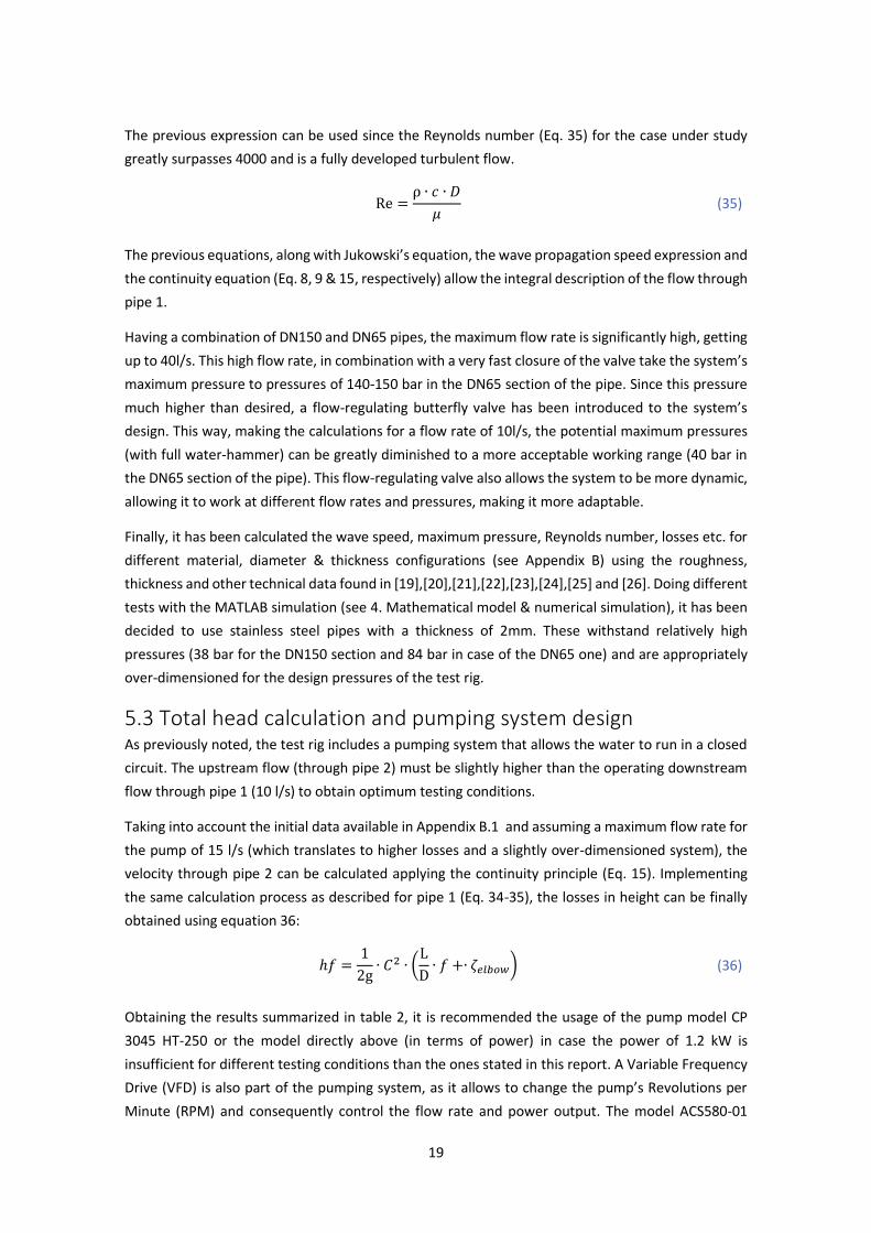
5.3 Total head calculation and pumping system design As previously noted, the test rig includes a pumping system that allows the water to run in a closed
circuit. The upstream flow (through pipe 2) must be slightly higher than the operating downstream
flow through pipe 1 (10 l/s) to obtain optimum testing conditions.
Taking into account the initial data available in Appendix B.1 and assuming a maximum flow rate for
the pump of 15 l/s (which translates to higher losses and a slightly over-dimensioned system), the
velocity through pipe 2 can be calculated applying the continuity principle (Eq. 15). Implementing
the same calculation process as described for pipe 1 (Eq. 34-35), the losses in height can be finally
obtained using equation 36:
ℎ𝑓 =1
2g∙ 𝐶2 ∙ (
L
D∙ 𝑓 +∙ 𝜁𝑒𝑙𝑏𝑜𝑤) (36)
Obtaining the results summarized in table 2, it is recommended the usage of the pump model CP
3045 HT-250 or the model directly above (in terms of power) in case the power of 1.2 kW is
insufficient for different testing conditions than the ones stated in this report. A Variable Frequency
Drive (VFD) is also part of the pumping system, as it allows to change the pump’s Revolutions per
Minute (RPM) and consequently control the flow rate and power output. The model ACS580-01

20
1.5kW VFD is also recommended, along with the Pumpte FL-06 level sensor for automatic start-stop
of the pump (see Appendix A).
5.4 Valve closure system For the DN65 fast-closing valve, it is important to specify and study the closure mechanism. The
requirements that the chosen mechanism should match consist on a fast closure time (0.5 seconds)
and the possibility of an easily adjustable speed closure, so different pressures and tests can be
performed.
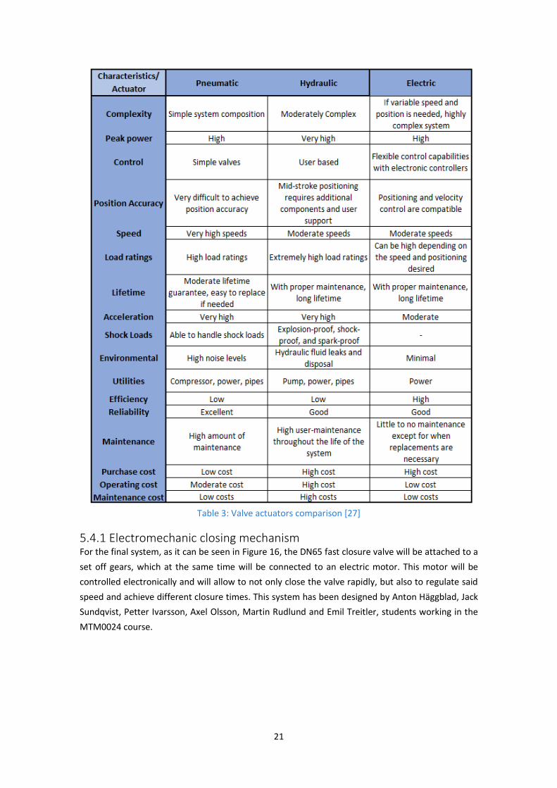
As per the possible closure mechanisms, there are a few systems that are usually used for fast-closing
valves. A comparison in between the most common of them is detailed in Table 3.
Taking into account this comparison & characteristics of the different possible mechanisms, it has
been decided to use an electric closing mechanism. This way, through the use of an electrical motor
and the installation of different gears, a fully electronically controlled system can be designed.
The type of valve for the fast-closure has been chosen to be a gate valve. These allow a much easier
simulation of their behavior and induced effects on the flow after a sudden momentum change.
Moreover, these valves are normally full-bore and they produce significantly low flow disturbance in
the system.
Table 2: Total head calculation results
Figure 115: CP 3045 HT-250 pump’s performance graph
21
Table 3: Valve actuators comparison [27]
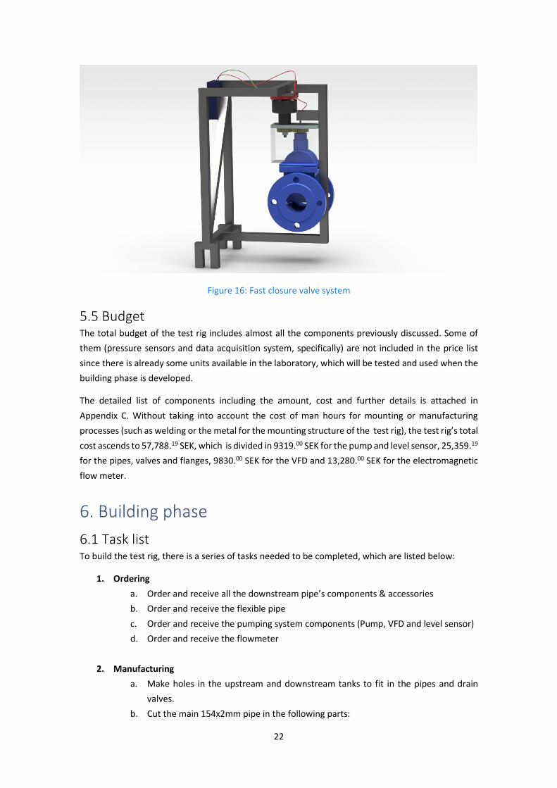
5.4.1 Electromechanic closing mechanism For the final system, as it can be seen in Figure 16, the DN65 fast closure valve will be attached to a
set off gears, which at the same time will be connected to an electric motor. This motor will be
controlled electronically and will allow to not only close the valve rapidly, but also to regulate said
speed and achieve different closure times. This system has been designed by Anton Häggblad, Jack
Sundqvist, Petter Ivarsson, Axel Olsson, Martin Rudlund and Emil Treitler, students working in the
MTM0024 course.
22
Figure 16: Fast closure valve system
5.5 Budget The total budget of the test rig includes almost all the components previously discussed. Some of
them (pressure sensors and data acquisition system, specifically) are not included in the price list
since there is already some units available in the laboratory, which will be tested and used when the
building phase is developed.
The detailed list of components including the amount, cost and further details is attached in
Appendix C. Without taking into account the cost of man hours for mounting or manufacturing
processes (such as welding or the metal for the mounting structure of the test rig), the test rig’s total
cost ascends to 57,788.19 SEK, which is divided in 9319.00 SEK for the pump and level sensor, 25,359.19
for the pipes, valves and flanges, 9830.00 SEK for the VFD and 13,280.00 SEK for the electromagnetic
flow meter.
6. Building phase
6.1 Task list To build the test rig, there is a series of tasks needed to be completed, which are listed below:
1. Ordering
a. Order and receive all the downstream pipe’s components & accessories
b. Order and receive the flexible pipe
c. Order and receive the pumping system components (Pump, VFD and level sensor)
d. Order and receive the flowmeter
2. Manufacturing
a. Make holes in the upstream and downstream tanks to fit in the pipes and drain
valves.
b. Cut the main 154x2mm pipe in the following parts:

23
i. Horizontal part 1 (HP1): to fit after the upstream tank
ii. Horizontal part 2 (HP2): to fit after the second elbow in the downstairs
laboratory(3.05m)
iii. Vertical part: which is at the same time divided in 2, a smaller 2.3m section
(VP1) and a 1m complement (VP2).
c. Manufacture the inner walls (separations) for the tanks, with the dimensions
specified in Appendix E.1.
d. Design and manufacture a mounting structure for the 154x2mm pipe.
e. Weld flanges on the ends of HP2.
f. Weld an elbow (EW1) with flanges in both of its ends.
g. Weld flanges to both ends of VP1.
h. Weld flanges to both ends of VP2.
i. Design and manufacture a structure to restrain both elbows in its position.
j. Weld flanges to both ends of the second elbow (EW2).
k. Weld both ends of HP1 with flanges.
l. Weld the concentric cones together and with flanges to both end of them or design
& manufacture a concentric cone structure with a 4° decrease, welding both ends
of it to flanges.
m. Cut the 69x2mm pipe in the following parts:
i. Horizontal pipe 3: A section of 1m (HP3)
ii. Horizontal parts 4-7: 3 sections of 30cms each one (HP4-7).
n. Weld flanges to both ends of HP3 and HP4-7.
o. Make the holes for the differential pressure sensors 30 cm away from either side of
the concentric cone.
p. Make the hole for the safety valve, which will be placed directly after the fast
closure valve.
q. Attach the 15mm copper tube to the safety valve and weld it to the whole made for
it, installing the safety valve.
r. Design and manufacture a system for closing the DN65 gate valve.
3. Installation
a. Organize the installation space in the downstairs lab, clean it up and remove all
elements that could interfere with the installation.
b. Install the inner walls (separations) in the upstream and downstream tanks.
c. Install the mounting structure for horizontal 154x2mm pipe, along with HP2 in the
downstairs lab.
d. Connect and screw HP2 with the EW1, aligning its vertical hole to the one in the
ceiling.
e. Install and screw VP1 to the vertical end of EW1, making sure it’s aligned with the
hole in the ceiling.
f. From upstairs, insert VP2, making it coincide with the end of VP1.
g. Install and screw EW2 to the upstairs’ end of VP2.
h. Restrain both elbows in its place and make sure the vertical pipe is immobilized.

24
i. Screw and install HP1 with EW2.
j. Screw and install the DN150 manual valve to one end of HP1 and the upstream tank.
k. Screw and install the concentric cone(s) to HP2.
l. Screw and install HP3 and HP4 with the electromagnetic flow meter, the fast closure
valve, the butterfly valve and the downstream tank.
m. Install the flexible pipe for downstream water, adjusting the valve and attaching it
to the upstream & downstream tanks.
n. Install the pump, along the corresponding system to control it (variable frequency
drive and control panel).
o. Install the flexible pipe for upstream water, from the pump to the upstream tank,
attaching the respective valve.
p. Install the differential pressure sensor with plastic small pipes connected to each of
the ends and holes made for this purpose.
q. Setup the Data Acquisition system for the pressure sensors.
r. Setup the fast closing valve with the electrical motor and gear system (see 5.3.1
Electromechanic closing mechanism)
s. Setup the level sensor in the downstream tank for the start-stop of the pump.
t. Install the drain valves in the bottom of both upstream and downstream tanks.
6.2 Planning These tasks are interdependent, which means that it is important to follow an ordered sequence to
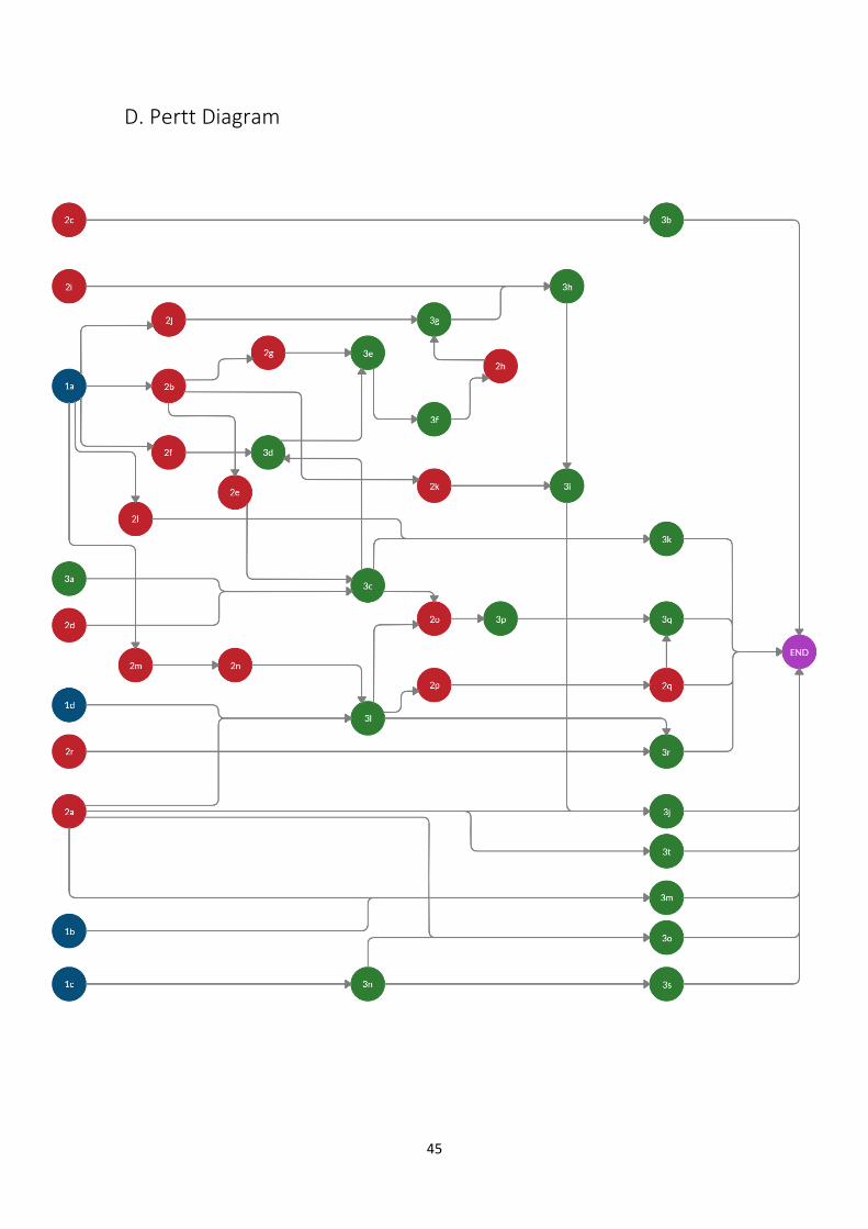
complete the building process. As can be seen in Appendix D, the Pertt diagram of the whole process
is fairly complex.
Following the principle of prioritizing the tasks that have the most dependent processes and
therefore doing them first, the final order that will be followed to complete the building process is:
1a, 1b, 1c, 1d, 3a, 2a, 2b, 2d, 2i, 2e, 3c, 2f, 3d, 2g, 3e, 3f, 2h, 2j, 3g, 3h, 2k, 3i, 3j, 2l, 3k, 2m, 2n, 3l,
3m, 3n, 3o, 2o, 3p, 2p, 2q, 3q, 2r, 3r, 3s, 2c, 3b, 3t.
Nonetheless, this doesn’t exclude the possibility of doing two or more tasks at the same time, with
the purpose of speeding up the process.
25
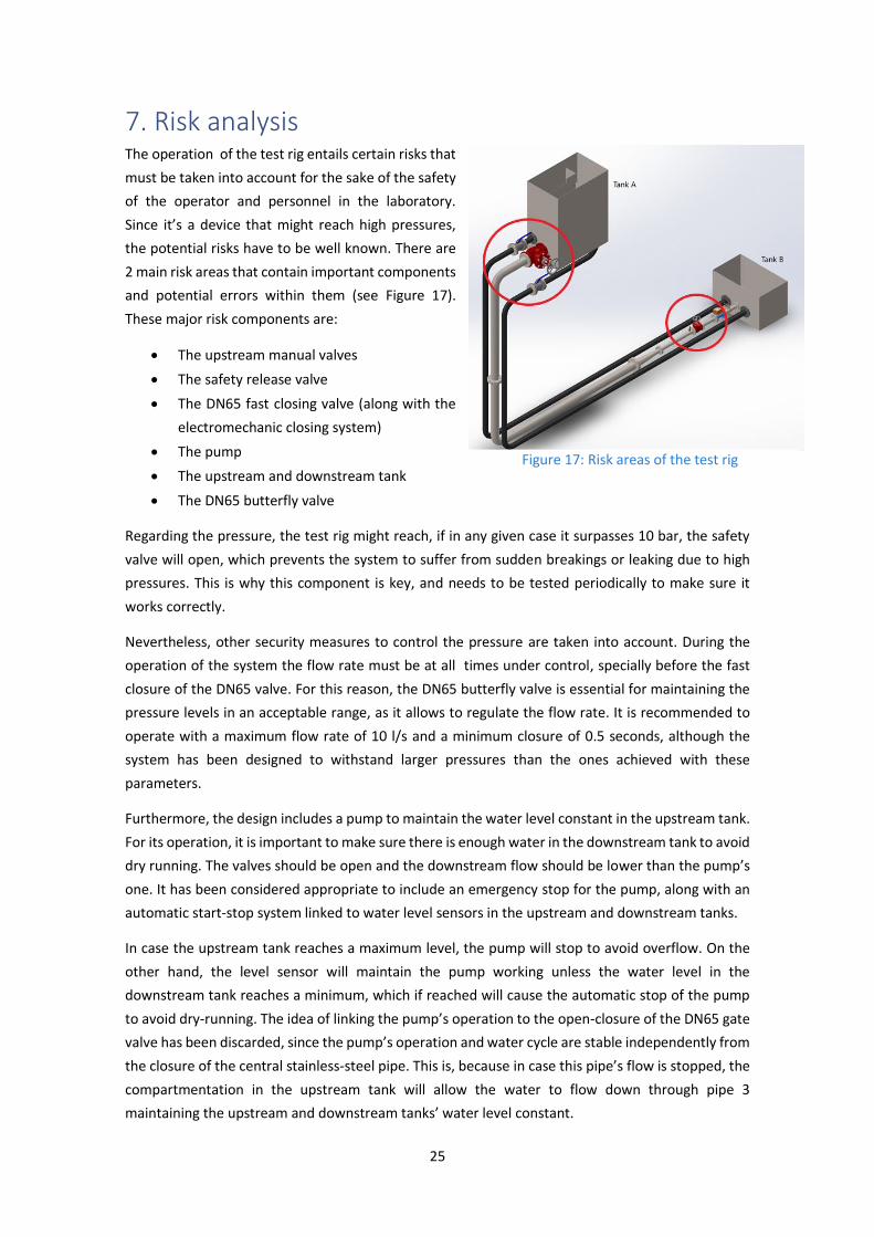
7. Risk analysis The operation of the test rig entails certain risks that
must be taken into account for the sake of the safety
of the operator and personnel in the laboratory.
Since it’s a device that might reach high pressures,
the potential risks have to be well known. There are
2 main risk areas that contain important components
and potential errors within them (see Figure 17).
These major risk components are:
• The upstream manual valves
• The safety release valve
• The DN65 fast closing valve (along with the
electromechanic closing system)
• The pump
• The upstream and downstream tank
• The DN65 butterfly valve
Regarding the pressure, the test rig might reach, if in any given case it surpasses 10 bar, the safety
valve will open, which prevents the system to suffer from sudden breakings or leaking due to high
pressures. This is why this component is key, and needs to be tested periodically to make sure it
works correctly.
Nevertheless, other security measures to control the pressure are taken into account. During the
operation of the system the flow rate must be at all times under control, specially before the fast
closure of the DN65 valve. For this reason, the DN65 butterfly valve is essential for maintaining the
pressure levels in an acceptable range, as it allows to regulate the flow rate. It is recommended to
operate with a maximum flow rate of 10 l/s and a minimum closure of 0.5 seconds, although the
system has been designed to withstand larger pressures than the ones achieved with these
parameters.
Furthermore, the design includes a pump to maintain the water level constant in the upstream tank.
For its operation, it is important to make sure there is enough water in the downstream tank to avoid
dry running. The valves should be open and the downstream flow should be lower than the pump’s
one. It has been considered appropriate to include an emergency stop for the pump, along with an
automatic start-stop system linked to water level sensors in the upstream and downstream tanks.
In case the upstream tank reaches a maximum level, the pump will stop to avoid overflow. On the
other hand, the level sensor will maintain the pump working unless the water level in the
downstream tank reaches a minimum, which if reached will cause the automatic stop of the pump
to avoid dry-running. The idea of linking the pump’s operation to the open-closure of the DN65 gate
valve has been discarded, since the pump’s operation and water cycle are stable independently from
the closure of the central stainless-steel pipe. This is, because in case this pipe’s flow is stopped, the
compartmentation in the upstream tank will allow the water to flow down through pipe 3
maintaining the upstream and downstream tanks’ water level constant.
Figure 17: Risk areas of the test rig
26
Finally, the electromechanic system attached to the DN65 fast-closing valve involves the need of
certain precautions, as it is designed to rotate and perform fast, high force movements, which could
harm any operator handling the gears, valve or engine. Before performing the fast closure of the
valve, it is necessary to make sure no personnel is handling this system.
8. Conclusions Throughout the design and realization of the project, an in-depth analysis of the water hammer
transient and pressure time method in a variable cross-section pipe has been carried. As far as the
previous calculations show, the cross-section variation in the pipe induces a variable water hammer
wave speed. This, in addition to the variation of the velocity of the flow itself (explained by the
continuity principle), has as a consequence the variation of the maximum pressure obtained through
a rapid momentum change (fast closure of the valve). The preliminary results indicate the maximum
pressure is considerably higher in the narrower part of the pipe.
Furthermore, given the small dimensions of the test rig, in comparison with full scale nuclear or
hydropower plants, a full water hammer (this is, having a low enough closure time so the maximum
Jukowski’s pressure is reached) is hardly attainable. The water hammer wave’s reflection time is too
low with a stiff material like stainless steel and the chosen thickness (2mm). Besides, for the purpose
of the Gibson method, the maximum Jukowski’s pressure is not mandatory.
For future developments on the area and potential studies of the pressure time method, a flow
regulation is strongly recommended. This allows to bound the resulting pressure wave of the system
to acceptable margins. It is also recommended the usage of gate or wedge valves for fast closure,
since its behavior and influence on the flow is more easily simulated through numerical methods or
flow analyzing software. Regarding its closure mechanism, if a variable closure time is desired, it is
recommended to use an electrical-based solution, since the electronic controllers for an engine are
well developed and allow a very precise control of the rotation speed.
Although the full design and planning of the test rig’s construction is detailed in this report, the
project had an unexpected turn of events due to the COVID-19 global pandemic and some renovation
works necessary in the laboratory that have led to the rescheduling of the building of the test rig.
This has pushed the present report to lack results from the testing and building, as the experimental
and hands-on phase has been delayed. Further follow-up of the current project is expected.
27
References [1] Swedish Energy Agency, “Energy in Sweden 2019, An Overview, Report no. ET 2019:3,” pp. 1–14,
2019.
[2] “Mechanical Autodata: Water Hammer and its Control,Devices.” [Online]. Available: http://autodata-engineer.blogspot.com/2011/03/water-hammer-and-its-controldevices.html. [Accessed: 19-Feb-2020].
[3] T. NIELSEN, “Dynamic Dimensioning of Hydro Power Plants,” 2001.
[4] “Pressure based Flow Meters - InstrumentationTools.” [Online]. Available: https://instrumentationtools.com/pressure-based-flowmeters/. [Accessed: 20-Feb-2020].
[5] “TN Instrumentation : ELECTROMAGNETIC FLOW METER.” [Online]. Available: http://tninstrumentation.blogspot.com/2014/03/electromagnetic-flow-meter.html. [Accessed: 20-Feb-2020].
[6] “RS Hydro stock Siemens 5100/6000 Magflo Meters.” [Online]. Available: https://www.rshydro.co.uk/flow-meters/siemens-magnetic-flow-meters/mains-powered-electro-magnetic-flowmeters/magflo-mag-5100w-flowmeter/. [Accessed: 21-Feb-2020].
[7] “An Innovative Approach to Applying the Pressure-Time Method to Measure Flow - Hydro Review.” [Online]. Available: https://www.hydroreview.com/2008/12/01/an-innovative-approach-to-applying-the-pressure-time-method-to-measure-flow/#gref. [Accessed: 21-Feb-2020].
[8] C. Purece, R. Zlatanovici, and S. Dumitrescu, “Hydro Turbine Flow Measurement By the Gibson Method ( Time – Pressure ),” vol. 75, no. 8, 2013.
[9] A. Adamkowski, “Discharge Measurement Techniques in Hydropower Systems with Emphasis on the Pressure-Time Method,” Hydropower - Pract. Appl., 2012, doi: 10.5772/33142.
[10] Y. A. Çengel and J. M. Cimbala, Fluid Mechanics: Fundamentals and applications, 1st ed. New York: Mc Graw Hill Higher Education, 2006.
[11] G. Dunca, D. M. Bucur, M. J. Cervantes, G. Proulx, and M. Bouchard Dostie, “Investigation of the pressure-time method with an unsteady friction,” in HYDRO 2013 - Promoting the Versatile Role of Hydro, 2013.
[12] G. Dunca, R. G. Iovanel, D. M. Bucur, and M. J. Cervantes, “On the use of the water hammer equations with time dependent friction during a valve closure, for discharge estimation,” J. Appl. Fluid Mech., vol. 9, no. 5, pp. 2427–2434, 2016, doi: 10.18869/acadpub.jafm.68.236.25332.
[13] P. P. Jonsson, J. Ramdal, and M. J. Cervantes, “Development of the Gibson method-Unsteady friction,” Flow Meas. Instrum., vol. 23, no. 1, pp. 19–25, Mar. 2012, doi: 10.1016/j.flowmeasinst.2011.12.008.
[14] A. Adamkowski and W. Janicki, “A new approach to calculate the flow rate in the pressure- time method – application of the method of characteristics,” HYDRO 2013 - Promot. Versatile Role Hydro, no. 1, 2013.
[15] M. Dalleli, M. A. Bouaziz, M. A. Guidara, E. Hadj-Taïeb, C. Schmitt, and Z. Azari, “Effect of water hammer on bent pipes in the absence or presence of a pre-crack,” Lect. Notes Mech. Eng., vol. 789, pp. 735–744, 2015, doi: 10.1007/978-3-319-17527-0_73.
[16] J. Carlsson, “Water Hammer Phenomenon Analysis using the Method of Characteristics and Direct Measurements using a ‘stripped’ Electromagnetic Flow Meter,” no. August, 2016.
[17] Sanda-Carmen Georgescu and Andrei-Mugur Georgescu, “Hydraulic Networks Analysis using GNU Octave,” Printech Press, Bucharest, Romania, Dec-2014. [Online]. Available: https://www.researchgate.net/publication/303805379_Calculul_Retelelor_Hidraulice_cu_GNU_

28
Octave_Hydraulic_Networks_Analysis_using_GNU_Octave_-_in_Romanian. [Accessed: 04-Mar-2020].
[18] S. Georgescu and A. Georgescu, “Fluid Flow in Pressurized Circular Pipes,” Ed. Printech, Bucharest, 2014.
[19] “Surface roughness of common materials - Table of reference values.” [Online]. Available: https://www.powderprocess.net/Tools_html/Data_Diagrams/Pipe_Roughness.html. [Accessed: 06-Jun-2020].
[20] E. ToolBox, “Roughness & Surface Coefficients,” 2003. [Online]. Available: https://www.engineeringtoolbox.com/surface-roughness-ventilation-ducts-d_209.html. [Accessed: 06-Jun-2020].
[21] S. Atlas, “Pressure Rating Table for Stainless Steel Tube,” 2011.
[22] Air-Way Global Manufacturing, “Steel Tubing Pressure Ratings,” 2018. [Online]. Available: https://www.air-way.com/resources/steel-tubing-pressure-ratings. [Accessed: 06-Jun-2020].
[23] Copper Devlopment Association, “The copper tube handbook,” 2006.
[24] Engineers Edge, “Pipe Roughness Coefficients Table Charts | Hazen-Williams Coefficient | Manning Factor - Engineers Edge.” [Online]. Available: https://www.engineersedge.com/fluid_flow/pipe-roughness.htm. [Accessed: 06-Jun-2020].
[25] “PVC Pipe Measurements OD, ID, Wall.” [Online]. Available: https://www.plasticpipeshop.co.uk/PVC-Pipe-Measurements-OD-ID-Wall_ep_53-1.html. [Accessed: 06-Jun-2020].
[26] Engineering ToolBox, “Young’s Modulus - Tensile and Yield Strength for common Materials,” 2003. [Online]. Available: https://www.engineeringtoolbox.com/young-modulus-d_417.html. [Accessed: 06-Jun-2020].
[27] “Advantages and Drawbacks of Pneumatic, Hydraulic, and Electric Linear Actuators.” [Online]. Available: https://www.timotion.com/en/news/news_content/blog_articles/general/advantages_and_drawbacks_of_pneumatic,_hydraulic,_and_electric_linear_actuators?upcls=1481266229&guid=1499762723. [Accessed: 24-Feb-2020].

29
Appendix
A. Retailers’ offers
A.1 Ahlsell: components

30

31
32

33

34
A.2. Ahlsell: Pump

35

36
A.3. Ventim: electromagnetic flow meter

37
A.4. Scandia Pumps: Level Sensor

38
A.5. ABB: Variable Frequency Drive
39
B. Excel calculations
B.1 Base parameters
B.2 Material, thickness and diameter comparison (straight pipe)

40

41
42
B.3 Maximum pressure with non-regulated flow
43
B.2 Maximum pressure with regulated flow

44
C. Budget
45
D. Pertt Diagram
E. 2D Planes
E.1 Plane 1: Detailed test rig
E.2 Plane 2: Additional components

1.6
0
1.30
6.0078
R0.30
0.7
5
0.725
1.00
3.3
0 R0.30
1.925
0.80
1.225
A
C
0.6078
2.35 3.05
D
B
M
0.148
0.4
0
0.2
5
0.394 DETAIL ASCALE 1 : 25
0.
104
0.
154
0.
104
0.
069
DETAIL DSCALE 1 : 25
0.367 0.246
0.2
5
DETAIL CSCALE 1 : 25
0.
10
0.1
57
0.15
0.025
0.025
1.00
0.5
38
0.2
5 0
.15
0.10
DETAIL BSCALE 1 : 25
0.025
0.025
1.2
2
0.7
2
0.10
0.1
32
0.1
13
DETAIL MSCALE 1 : 25
A A
B B
C C
D D
E E
F F
8
8
7
7
6
6
5
5
4
4
3
3
2
2
1
1
UNLESS OTHERWISE SPECIFIED:DIMENSIONS ARE IN METERS
MATERIAL:
TITLE:
DRAWN BY
SCALE:1:50 SHEET 1 OF 2
A3
DATE: JUNE 2020
E.1 Plane 1: Detailed Test Rig
Joan Mateu Chiquin FontStainless Steel & Flexible PVC

F
F
E
E
0.4
5 0.20
1.4
0
G
L
SECTION E-E
0.2
0
H
SECTION F-F
0.05
0.20
0.1
5
DETAIL GSCALE 1 : 20
0.108
0.065
DETAIL HSCALE 1 : 15
0.6
5 0.7
5
0.0
65
0.4
5
0.14 DETAIL L
SCALE 1 : 25
Stainless Steel & Flexible PVC
A A
B B
C C
D D
E E
F F
8
8
7
7
6
6
5
5
4
4
3
3
2
2
1
1
MATERIAL:
TITLE:
DRAWN BY:
SCALE:1:50 SHEET 2 OF 2
A3
DATE: JUNE 2O2O
E.1 Plane 1: Detailed Test RigUNLESS OTHERWISE SPECIFIED:DIMENSIONS ARE IN METERS
Joan Mateu Chiquin Font

0.18 0.33 0.65 0.65 0.61 3.00
A
0.03
DETAIL ASCALE 1 : 10
A A
B B
C C
D D
E E
F F
8
8
7
7
6
6
5
5
4
4
3
3
2
2
1
1
DIMENSIONS ARE IN METERS UNLESSSPECIFIED OTHERWISE
TITLE:
DRAWN BY:
SCALE:1:50 SHEET 1 OF 1
A3
DATE: JUNE 2020
Joan Mateu Chiquin Font
E.2 Plane 2: Additional components
MATERIAL:
Stainless Steel &Flexible PVC
Top Related