Periodically driven perturbed CFTs: the sine-Gordon model

Zoltán Bajnok1, Robin Oberfrank1,2

August 23, 2021

1Wigner Research Centre for PhysicsKonkoly-Thege Miklós u. 29-33, 1121 Budapest, Hungary

2Roland Eötvös UniversityPázmány s. 1/A, 1117 Budapest, Hungary

Abstract

We analyze a version of the sine-Gordon model in which the strength of the cosinepotential has a periodic dependence on time. This model can be considered as the con-tinuum limit of the many body generalization of the Kapitza pendulum. Based on theperturbed CFT point of view, we develop a truncated conformal space approach (TCSA)to investigate the Floquet quasienergy spectrum. We focus on the effective behaviour forlarge driving frequencies, which we also derive exactly. Depending on the driving pro-tocol, we can recover the original sine-Gordon model or its two-frequency version. Therich structure of the two-frequency model implies that the time-periodic drive can breakintegrability, can lead to new states in the spectrum or can result in a phase transition.Our method is applicable for any periodically driven perturbed conformal field theories.

1

arX

iv:2

107.

1308

0v2

[he

p-th

] 2

0 A

ug 2

021

Contents

1 Introduction 2

2 Classical considerations 32.1 Kapitza pendulum . . . . . . . . . . . . . . . . . . . . . . . . . . . . . . . . . . 42.2 Many body generalization: the sine-Gordon model . . . . . . . . . . . . . . . . 5

3 Quantum models 73.1 Floquet theory and the Kapitza pendulum . . . . . . . . . . . . . . . . . . . . . 73.2 The periodically driven sine-Gordon model . . . . . . . . . . . . . . . . . . . . . 8

3.2.1 Sine-Gordon model as a perturbed CFT . . . . . . . . . . . . . . . . . . 93.2.2 Periodic drive . . . . . . . . . . . . . . . . . . . . . . . . . . . . . . . . . 10

4 Numerical investigations and results 124.1 Floquet quasienergy spectrum . . . . . . . . . . . . . . . . . . . . . . . . . . . . 124.2 Effective Hamiltonian . . . . . . . . . . . . . . . . . . . . . . . . . . . . . . . . 14

5 Periodically driven perturbed CFTs 17

6 Conclusion 18

A Large frequency expansion and a numerical approach 20

B TCSA and the driven sine-Gordon model 21

C Calculation of the effective Hamiltonian for generic pertrubed CFTs 25

1 Introduction

The equilibrium behaviour of isolated statistical physical systems are successfully describedand understood [1]. Recently, the focus of the investigations has been shifted to the far fromequilibrium domain, partly due to the advancement of cold atom experiments. By introducingvarious protocols, the system can be driven away from the equilibrium and the main problem isto understand its long time behaviour. Typically, we let the originally closed quantum systemto interact with its environment. This can be a sudden change in the boundary conditions orin the parameters of the theory and often we close the system again after this quench and weinvestigate the relaxation towards equilibrium [2].

Alternatively, we can subject the system to a periodic driving force and investigate itstime evolution. In many cases, the driven interacting system becomes ergodic and visitsthe whole phase space in the classical case or heats to infinite temperature in the quantumcase. However, there is a large class of models when this does not happen and the systemremains stable. The periodic drive can lead to universal high frequency behaviour, which leadsto dynamical stabilization and can be used in Floquet engineering, a topic very intensivelyinvestigated recently [3].

A particularly interesting case is when the originally unstable fix points become stable. Aprototypical example is the Kapitza pendulum [4], a rigid pendulum in which the pivot point is

2

moved harmonically in the vertical direction. For large enough driving frequencies the upperunstable equilibrium point can be dynamically stabilized by this periodic drive. The fieldtheoretical limit of the many-body generalization of the Kapitza pendulum is the periodicallydriven sine-Gordon model [5], which was analyzed by various approximate methods and thedynamical stability was indicated. The authors also suggested an experimental realization inan ultracold atom experiment, in which the atoms are trapped into two parallel one dimensionallines by a transversal confinement potential generated through standing laser waves. Bymodulating the amplitude of the transverse field a time-dependent tunneling coupling betweenthe two parallel tubes can be induced realizing the drive needed for the sine-Gordon model.

In the present paper, we would like to go beyond the methods and the focus of [5] andwould like to analyze the quasienergy spectrum of the driven sine-Gordon theory. This will bedone by exploiting that the sine-Gordon theory can be considered as a perturbed conformalfield theory (CFT). This allows us to use analytical and very successful numerical methodsto investigate the system. The truncated conformal space approach (TCSA) [6] proved tobe a useful tool to analyze various observables in perturbed conformal field theories and ouraim is to combine it with the usual numerical method of the periodically driven systems tocalculate the spectrum of the Floquet Hamiltonian. We are going to identify a protocol whenthe infinite frequency effective theory becomes the two-frequency sine-Gordon model [7, 8]allowing us to see the dynamical stabilization of unstable fix points and reach very nontriviallimiting theories. Our approach paves the way to investigate periodically driven perturbedconformal field theories with the same methods. In the formulation of our approach we takea pedagogical path and introduce all concepts in simplified circumstances.

The paper is organized as follows: we start in section 2 by recalling the dynamical sta-bilization and separation of time scales in the example of the Kapitza pendulum, which isbasically the zero mode of the driven sine-Gordon theory. We also emphasize the possibility ofintroducing different driving protocols, depending on how we scale the amplitude of the drivewith the frequency. By coupling many Kapitza pendula and taking their continuum limit, wearrive at the driven sine-Gordon theory, whose stability we analyze in the small amplitudelimit, where we can see that stability can be ensured only in a finite volume or with a momen-tum cutoff. We then turn to the quantum theory in section 3. Floquet theory, the quantumapproach to periodically driven systems is introduced on the example of the quantum Kapitzapendulum, together with the standard numerical method based on Fourier transformation tocalculate the quasienergy spectrum and an analytical method to derive the large frequencyexpansion [9]. Having introduced the sine-Gordon theory as a perturbed CFT together withits TCSA method [10], we specify the previous findings to deal with the periodical drive. Wealso perform analytical calculations and reveal the importance of scaling the amplitude of thedrive. The numerical investigations and their interpretations are summarized in section 4.The analytical calculation for the large frequency effective behaviour is extended for genericperturbed conformal field theories in Section 5. Finally, we conclude in section 6. Technicaldetails are relegated to Appendices.

2 Classical considerations

In this section, we review the classical theory and introduce the separation of scales as well asthe large frequency expansion.

3

2.1 Kapitza pendulum

The Kapitza pendulum is a rigid pendulum in which the pivot point is moved harmonicallyin the vertical direction [4]. The Hamiltonian has the form

H =p2φ

2+ c(t)(1− cosφ) ; c(t) = c0 + c1 cosωt (1)

where φ is the 2π periodic angle variable and the driving is controlled by c1. Without thedrive, the system has two equilibrium points: φ = 0 is stable, while φ = π is unstable.For large enough driving frequencies, however, the unstable fix point becomes stable. Thiscounterintuitive phenomenon can be understood in the effective description, in which themotion is separated into an average slow and a periodic fast motion

φ(t) = Φ(t) + ξ(t) ; ξ(t+ T ) = ξ(t) (2)

where T = 2πω and

´ t+T/2t−T/2 φ(t)dt = Φ(t). There is a systematic expansion in ω−2, see [9] for

details, which at the leading order gives

ξ =c1

ω2cosωt sin Φ ; Φ = − d

dΦ

(c0(1− cos Φ) +

c21

4ω2sin2 Φ

)≡ −dUeff(Φ)

dΦ(3)

Thus, there is a small-amplitude, large-frequency motion with vanishing time average and aslow motion in an effective potential. The new term in the effective potential makes the upperequilibrium point stable as demonstrated on Figure 1.

Figure 1: Periodic motion around the upper equilibrium point obtained by solving the equationof motions with the periodic drive, and the corresponding effective potential.

Depending on how the amplitude of the drive scales with ω, we can see different behaviours:

• For ω-independent c1 = λ, the drive averages out in the large ω limit, and the effectivemotion is the same as the one without the drive. It can be understood physically as thedrive is oscillating so fast so that the system with a finite inertia cannot follow it.

4

• This is drastically changed if the drive scales with ω: c1 = λω. In this case, the fastoscillation vanishes in the large ω limit, and the motion is basically as it would happenin the effective, ω-independent potential Ueff(Φ) = c0(1−cos Φ)+ λ2

4 sin2 Φ. For λ2

2 > c0,both equilibria are stable.

• In the case of the Kapitza pendulum the drive is proportional to ω2: c1 = λω2. Thesmall fluctuations are ω-independent, but the effective potential does not have a finiteω →∞ limit. In this case, ω is kept finite and the system has a rich stability diagram.

The stability of the two equilibria can be understood in the small-angle limit, φ ∼ ε, π+ ε, i.esinφ ∼ ±ε when the equation of motion can be mapped to the Mathieu equation

y′′(x) + (a− 2q cos 2x)y(x) = 0 ; (a, q, x)↔(±4c0

ω2,2c1

ω2,ωt

2

)(4)

with a well-known stability diagram (see Figure 2). The upper equilibrium appears for a < 0,while the lower one for a > 0. Clearly, for the Kapitza pendulum c1 = λω2, the upper fixpoint becomes stable above a λ-dependent critical frequency.

Figure 2: Stability diagram of the Mathieu equation. Stable regions correspond to boundedoscillations, while unstable ones mean exponentially growing solutions.

In the following sections, we focus on the case when the effective potential has a finitenon-trivial ω →∞ limit, and investigate the continuum limit of the many body generalizationof this model.

2.2 Many body generalization: the sine-Gordon model

If we take many pendula on a line, couple them with torsion springs and take the continuumlimit we obtain the sine-Gordon field theory with infinite degrees of freedom, see eg. [11].Doing the same with many Kapitza pendula leads to the driven sine-Gordon model [5]:

∂2t φ(x, t)− ∂2

xφ(x, t) + (c0 + c1 cosωt) sinφ(x, t) = 0 (5)

5

The stability of the system around the φ(x, t) = 0, π configurations can be analyzed by ap-proximating sinφ ∼ ±φ and decoupling the modes in Fourier space. The resulting equationof motion for the kth mode φ(x, t) ∝ φk(t)eikx can again be mapped to the Mathieu equation

∂2t φk ± (c0 ± k2 + c1 cosωt)φk = 0 ; (a, q)↔

(4±c0 + k2

ω2,2c1

ω2

)(6)

Figure 3: Small fluctuations of the periodically driven sine-Gordon equation are mapped tothe stability diagram of the Mathieu equation for various parameters. Red lines correspond toevolving field configurations with resonant modes, green ones have stable evolution. Left figureshows solutions localized to the lower fix point, where the momentum cutoff is not necessary,while on the right, we see solutions localized to the upper fix point, where the cutoff has tobe used to avoid the resonant modes.

Since in the field theory, we have a continuum of modes k ∈ R, whatever c0 and c1 wechoose we always cross the instability regions, see Figure 3. The reason is that in our small-fielddecoupled harmonic oscillator limit, we always have a mode, which resonates with the drivingfrequency leading to parametric resonance. To avoid this, we could put the system in a finitevolume L, and then the possible k values will be quantized: kn = n2π

L , and we might avoidthe discrete points that lie within the unstable regions. In the large volume limit, however,we should always face some instabilities. We could also introduce a momentum cutoff kmax,and choose a large enough driving frequency, such that the corresponding allowed (a, q) valuesalways lie in the stability region. This is actually the typical case as in many applications, thesine-Gordon model is an approximation, and the real physical system has a built in ultra-violetcutoff.

With this trick, we can even make the upper fix point, φ = π stable. This configurationthen can serve as another vacuum and excitation such as the breather can live over them.We demonstrate this by explicitly solving the equation of motion (see Figure 2.2). In ourapproach, we used the Chebyshev spectral method to calculate the time evolution.

It is a conceptually interesting question whether the stability survives in the quantumtheory or not. Clearly at the quantum level, the excitations are quantized and they cannotbe arbitrarily small, thus the small φ expansion is not adequate. Indeed, in the sine-Gordontheory, the small fluctuations correspond to breather excitations, which are the elementary

6

Figure 4: Time evolution of a breather type configuration at the upper fix point with param-eters: c1 = λω2, λ = 0.1, ω = 100, c0 = 1. This configuration does not decay, but slowlyradiates due to non-integrable effects [12].

quanta of the field with finite masses. Depending on the coupling, the masses vary andthe breathers can even leave the spectrum, such that only solitons remain. This makes thequantum theory stable as we will see. In the quantum analyzis, we will introduce both a finitevolume and a momentum cutoff, and will focus on the large-frequency limit, varying both thevolume and the cutoff, too.

3 Quantum models

In this section, we introduce the Floquet theory of periodically driven systems together withtheir large frequency expansion and develop a numerical method to investigate the spectrumof the quasienergies. We start with the quantum version of the Kapitza pendulum. We thenpresent the sine-Gordon theory, where we exploit its perturbed CFT formulation.

3.1 Floquet theory and the Kapitza pendulum

In the quantum theory, we investigate the time evolution of the system with an explicitharmonic-type time-dependent Hamiltonian

i∂Ψ

∂t= HΨ ; H = H0 + V0 + cosωt V1 (7)

i.e. V0, V1 will not depend explicitly on time. In the case of the Kapitza pendulum, they takethe form

H0 =p2φ

2; V0 = c0(1− cosφ) ; V1 = c1 cosφ (8)

The separation of scales has a quantum analogue [9], which is phrased in Floquet theorem:for periodic Hamiltonians H(t) = H(t + T ) the solution of the Schrödinger equation can beexpanded in a basis ψE evolving as

ψE(φ, t) = e−iEtuE(φ, t) (9)

7

where uE(φ, t + T ) = uE(φ, t). The quasienergy E governs the slow motion in an effectivepotential, while the periodic uE is the analogue of the fast modulation. In order to find theeffective Hamiltonian, which is unitary equivalent to the operator that generates the evolutionwith one period of time, one can make a periodic gauge transformation [9] of the form uE(φ, t) =e−iF (t)vE(φ) leading to

Heff = eiFHe−iF − i(∂teiF )e−iF (10)

where F and Heff can be calculated simultaneously order by order in ω−1, see appendix A,and at the leading and non-vanishing subleading order we get

Heff = H0 + V0 +1

4ω2[[V1, H0 + V0], V1] +O(ω−4) (11)

This calculation is quite general, which relies only on the specific time dependence of theperturbation cosωt V1, but not on the specific form of V0, V1 and will be valid also in thequantum field theory. In the generic case of a single particle, the effective Hamiltonian is

Heff =p2φ

2+ V0 +

1

4ω2(∂φV1)2 +O(ω−4) (12)

Clearly, for the Kapitza pendulum, this yields the same effective potential Ueff as in (3), whichis the quantum analogue of the classical dynamics. In the more general case when V0 and V1

are equivalent up to a linear term in the coordinate, this maps all unstable fix points of V0 tostable ones.

In order to test the above large-frequency approximation, we can determine numericallythe Floquet basis, which satisfies the modified Schrödinger equation:

HFuE(φ, t) = EuE(φ, t) ; HF = H − i∂t (13)

Since uE(φ, t) is periodic in time, we simply expand it in Fourier components: uE(φ, t) =∑m uE,m(φ)eimωt such that the eigenvalue problem takes the form

(mω +H0 + V0)uE,m +1

2V1(uE,m−1 + uE,m+1) = EuE,m (14)

We can further expand uE,m(φ) in the eigenbasis of H0, and formulate an equation in thedouble discrete infinite basis, see Appendix A for details. The numerical solution showed(see Figure 5) that for large ω, the effective description is recovered correctly, and from theeigenvectors, we can recognize states localized around the upper equilibrium point.

3.2 The periodically driven sine-Gordon model

The quantum version of the periodically driven sine-Gordon model shares the same stuctureof the Hamiltonian as the Kapitza pendulum (7) but we are in a quantum field theory wherethe system is confined into a finite volume L as

H0 =1

8π

ˆ L

0dx : (∂tφ)2 − (∂xφ)2 : ; Vi = ci

ˆ L

0dx : cosβφ : (15)

and the normal ordering is defined wrt. the free compactified massless boson of radius r = β−1

[10, 11].

8

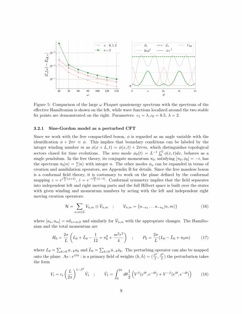
Figure 5: Comparison of the large ω Floquet quasienergy spectrum with the spectrum of theeffective Hamiltonian is shown on the left, while wave functions localized around the two stablefix points are demonstrated on the right. Parameters: c1 = λ, c0 = 0.5, λ = 2.

3.2.1 Sine-Gordon model as a perturbed CFT

Since we work with the free compactified boson, φ is regarded as an angle variable with theidentification φ + 2πr ≡ φ. This implies that boundary conditions can be labeled by theinteger winding number m as φ(x + L, t) = φ(x, t) + 2πrm, which distinguishes topologicalsectors closed for time evolutions. The zero mode φ0(t) = L−1

´ L0 φ(x, t)dx, behaves as a

single pendulum. In the free theory, its conjugate momentum π0, satisfying [π0, φ0] = −i, hasthe spectrum π0|n〉 = n

r |n〉 with integer n. The other modes φn can be expanded in terms ofcreation and annihilation operators, see Appendix B for details. Since the free massless bosonis a conformal field theory, it is costumary to work on the plane defined by the conformalmapping z = ei

2πL

(x+t), z = e−i2πL

(x−t). Conformal symmetry implies that the field separatesinto independent left and right moving parts and the full Hilbert space is built over the stateswith given winding and momentum numbers by acting with the left and independent rightmoving creation operators:

H =∑n,m∈Z

Vn,m ⊗ Vn,m ; Vn,m = {a−n1 . . . a−nk |n,m〉} (16)

where [an, am] = nδn+m,0 and similarly for Vn,m with the appropriate changes. The Hamilto-nian and the total momentum are

H0 =2π

L

(L0 + L0 −

1

12+ π2

0 +m2r2

4

); P0 =

2π

L(L0 − L0 + π0m) (17)

where L0 =∑

k>0 a−kak and L0 =∑

k>0 a−kak. The perturbing operator can also be mappedonto the plane. As : eiβφ : is a primary field of weights (h, h) = (β

2

2 ,β2

2 ) the perturbation takesthe form

Vi = ci

(L

2π

)1−β2

V1 ; V1 =

ˆ 2π

0dθ

1

2

(V β(eiθ, e−iθ) + V −β(eiθ, e−iθ)

)(18)

9

where the normal ordered vertex operator on the plane was introduced V β(z, z) =: eiβφ(z,z) :.Without the drive, c1 = 0, normal ordering is enough to regularize the theory for β2 < 1.In this region, the theory contains breather and soliton excitations. The only dimensionfulperturbing parameter c0 sets the scale and it is related to the soliton mass M as [13]:

c0 = κ(h)M2−2h ; κ(h) =2Γ(h)

πΓ(1− h)

(√πΓ( 1

2(1−h))

2Γ( h2(1−h))

)2−2h

(19)

The truncated conformal space approach can be used the calculate the spectrum [6]. Itamounts to truncate the Hilbert space at a given energy, Ecut, and to calculate the finitematrix representations of the Hamiltonian H0 + V0 and then diagonalize them [10]. A typicalspectrum can be seen on Figure 6.

Figure 6: Typical TCSA spectrum of the sine-Gordon theory. Here and from now on we alwayschoose r = 3, M = 1. On the left is the raw spectrum, while on the right we subtract theexactly known bulk groundstate energy. Breather masses are indicated by dashed lines.

Since this is an integrable quantum field theory, the finite size spectrum is completelyknown [14, 15]. The bulk energy constant is ebulk = −M2

4 tan πp2 , where h = p

1+p = β2

2 , whilethe mass of the kth breather is mk = 2M sin πpk

2 .For 1 < β2 the perturbing operator is not well-defined [16]. The spectrum does not stabilize

in the Ecut → ∞ limit and one has to subtract an Ecut-dependent diverging constant. Thiscan be avoided by analyzing energy differences only. For higher βs, even energy differencesare not enough to consider and one has to introduce an Ecut-dependent operator counter term[16, 17]. Above β2 = 2, the TCSA method cannot be used, as we cross the Kosterlitz-Thoulessphase transition and the perturbation becomes irrelevant.

3.2.2 Periodic drive

Let us now analyze the effect of the periodic drive. If the drive is turned on, we are inter-ested in the Floquet quasienergy spectrum. The large ω expansion follows the calculation ofthe Kapitza pendulum and leads to the effective Hamiltonian (11), which in dimensionless

10

quantities in our case reads as

Heff =2π

L

[H0 +

c0

2

(L

2π

)2−β2

V1 +

(L

2π

)2−2β2

c21

4ω2[[V1, H0], V1]

]+O(ω−4) (20)

We calculate the commutator [[V1, H0], V1] in Appendix B analytically. As the expressioncontains products of operators at the same points, the commutator is not well-defined andneeds to be regularized. By introducing a mode number cutoff, we keep only the oscillatorswith mode numbers between −nmax and nmax. As a result, the regularized commutator hasthe structure

[[V1, H0], V1]cut ∝ an2β2

maxI + n−2β2

max V2 +O(n−2β2−1max ) (21)

where V2 corresponds to a perturbation with double frequency:

V2 =

ˆ 2π

0

dθ

2

(V 2β(eiθ, e−iθ) + V −2β(eiθ, e−iθ)

)(22)

The contribution of the identity operator is diverging in the limit when the cutoff is eliminated(ncut → ∞) and should be renormalized. This can be easily done by considering energydifferences only, and then the large ω behaviour can be different depending on how we scalec1. We expect the following behaviours:

• If c1 is not scaled with ω, c1 = λ, then the drive averages out and we should see no effectin the spectrum.

• If c1 is scaled with ω, c1 = λω, then we have an effective large ω behaviour, which inenergy differences appears as the spectrum of the two-frequency sine-Gordon model. Byeliminating the regulator ncut → ∞, the extra cos 2βφ term in the effective potentialscales to zero and we again should get back the spectrum of the sine-Gordon theory.

• If, however, we also scale the bare coupling c1 with the regulator as c1 = λωEβ2

cut, inorder to compensate the factor n−2β2

max , then we have a nontrivial large ω and Ecut →∞limit. In this limit, the volume dependence of the new term in the effective potential is(

L

2π

)1−4β2

λ2

4

(EcutL

2π

)2β2

[[V1, H0], V1] (23)

where the dimensionless cut Ecut = EcutL2π is the analogue of nmax in this scheme and

E2β2

cut [[V1, H0], V1] has a finite limit corresponding to the double-frequency cosine opera-tor. The effective theory should then be the two-frequency sine-Gordon model [8]:

Heff =2π

L

[H0 + c0

(L

2π

)2−β2

V1 +

(L

2π

)2−4β2

c2V2

](24)

where c2 ∝ λ2 is a scheme-dependent renormalized coupling.

In order to check these behaviours, we develop a novel numerical method. The idea is to com-bine TCSA with the numerical approach we used in the quantum mechanical case. We thus ex-pand in Fourier components the periodic Floquet wave function in time uE(t) =

∑m uE,me

imωt

11

and solve the Floquet eigenvalue problem (14) but keeping in mind that now the operartorsH0, V0 and V1 act on the conformal Hilbert space. We use the TCSA method to represent theseoperators with finite matrices on the truncated Hilbert space. Since both the winding numberand the momentum is preserved by the perturbation, we focus on the m = 0 and P = 0sector. The relevant matrix element of the perturbation are described in Appendix B. In thefollowing section we summarize our findings. All physical quantities are made dimensionlessby the soliton mass M .

4 Numerical investigations and results

In this section, we solve numerically both the time-dependent theory at high but finite fre-quency, and its corresponding time-independent effective theory to support our claims. For adetailed description of the used methods, see Appendix (B).

Figure 7: The difference between the quasienergies of the driven and the energies of the originalsine-Gordon model for the vacuum and for the first excited state for various c1 = λ values asthe function of ω at volume ML = 14.

4.1 Floquet quasienergy spectrum

Our first goal is to confirm that the high-frequency expansion is also valid in the continuumlimit. In the case when c1 = λ, the expansion tells us that the full perturbation vanishes in thehigh-frequency limit, therefore, from the quasienergies, we should obtain the spectrum of theintegrable sine-Gordon theory. This is exactly what we see in Figure 7. Here, we show thatfor the vacuum (n = 0) and the first standing particle (n = 1), the difference of the energiestends to zero as the frequency increases independently of the strength of the perturbation.

Let us now turn to the c1 = λω case, where we expect a non-trivial behaviour due to theeffect of the λ2

4 [[V1, H0], V1] operator. Looking at the full spectrum on Figure 8, we can seethat it resembles a meaningful quantum field theory. Knowing that we are in the m = 0,P = 0 sector, we can identify the vacuum, the standing particles, and the scattering states.

12

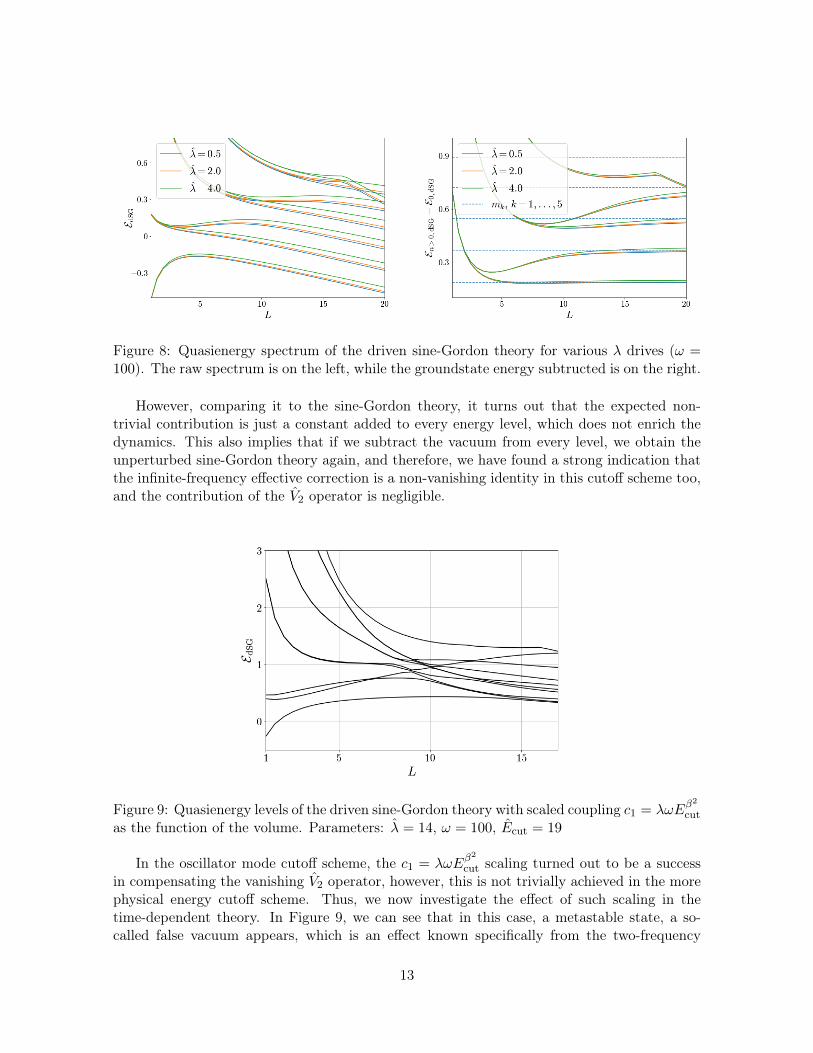
Figure 8: Quasienergy spectrum of the driven sine-Gordon theory for various λ drives (ω =100). The raw spectrum is on the left, while the groundstate energy subtructed is on the right.

However, comparing it to the sine-Gordon theory, it turns out that the expected non-trivial contribution is just a constant added to every energy level, which does not enrich thedynamics. This also implies that if we subtract the vacuum from every level, we obtain theunperturbed sine-Gordon theory again, and therefore, we have found a strong indication thatthe infinite-frequency effective correction is a non-vanishing identity in this cutoff scheme too,and the contribution of the V2 operator is negligible.

Figure 9: Quasienergy levels of the driven sine-Gordon theory with scaled coupling c1 = λωEβ2

cut

as the function of the volume. Parameters: λ = 14, ω = 100, Ecut = 19

In the oscillator mode cutoff scheme, the c1 = λωEβ2

cut scaling turned out to be a successin compensating the vanishing V2 operator, however, this is not trivially achieved in the morephysical energy cutoff scheme. Thus, we now investigate the effect of such scaling in thetime-dependent theory. In Figure 9, we can see that in this case, a metastable state, a so-called false vacuum appears, which is an effect known specifically from the two-frequency

13

sine-Gordon model [8]. The false vacuum is a vacuum-like energy eigenstate (with linearvolume dependence) that has a higher bulk energy, and in this case, we can interpret it as theanalogue of the stabilized upper fix point of the Kapitza pendulum. This state can exist ina finite volume., andfor larger and larger volumes, it approaches a particle line over the realvacuum. Since this theory is not integrable, the lines avoid each other and the metastablevacuum decays.

Unfortunately, in the parameter region where the time-dependent theory shows the sta-bilization effect the simulations become more resource demanding and we could not achievegood enough precisions. In order to overcome this, we compare the time-dependent Floquetspectrum to that of the effective time-indepent theory.

In Figure 10, we can see the same behaviour as we have seen in the quantum mechanicalcase (Figure 5): solving the time-dependent Floquet problem and the time-independent effec-tive theory yields the same energies towards the high-frequency limit. We thus in the nextsubsection focus on a precision analyzis of the spectrum of the effective Hamiltonian.

Figure 10: The difference between the quasienergies of the driven and energies of the effectiveHamiltonian (20) for the vacuum and the first excited state for various c1 = λω values as thefunction of ω at dimensionless volume ML = 14.

4.2 Effective Hamiltonian

In this section, we analyze the cases when the drive is scaled with the frequency c1 = λω andω goes to ∞. The effective Hamiltonian in this limit takes the form

Heff

M=

2π

ML

[H0 +

κ(β2/2)

2

(ML

2π

)2−β2

V1 +

(ML

2π

)2−2β2

λ2

4[[V1, H0], V1]

](25)

where we made the expression dimensionless by dividing by the soliton mass and λ is thecorresponding dimensionless coupling. The TCSA method truncates the Hilbert space at agiven energy cut Ecut and represents all operators on this truncated Hilbert space by finite

14

dimensional matrices. As a consequence, the commutator [[V1, H0], V1] is finite, thus regular-ized, but its matrix elements depend on the energy cutoff. We note that this regularizationis not the same which we used in Appendix (B), where we truncated the Hilbert space in theoscillator types (mode numbers) and not in the energy. In that case, arbitrarily large energystates could contribute with small mode numbers.

Figure 11: Diagonal elements of the commutator at different energy cuts, when projectedback to the Hilbert space at cut = 6. We see that at a given L0 eigenspace, we basically havean identity operator, however, the relative cutoff dependences of the different L0 eigenspacesare slightly different and are shifted wrt. each other. The gap between different identitycoefficients scales to zero for larger and larger cuts as shown on the left inset. On the rightinset we can see how the coefficient of the identity scales with the cut.

In order to understand the cutoff dependence of the commutator, we analyze its matrix ele-ments. Technically, we choose a cutoff and construct the corresponding Hilbert space togetherwith the matrix elements of [[V1, H0], V1]. In the next step, we increase the cutoff as well as therepresentations of H0 and V1 but focus only on the same matrix elements of [[V1, H0], V1]. Wecompare the resulting matrix elements to that of the operators I and V2. The Hilbert space hasa tensor product form composed of the zero mode and the other oscillators. The commutatorin the zero mode space has elements in the diagonal and the second super/subdiagonal blocks,but none of them depends on the value of the zero mode. This enables us to investigate thecommutator on a Hilbert space with keeping only the n = −1, 0, 1 sectors. We then analyzethe cutoff dependence in the other oscillators. In our convention, the cut is an integer whichdetermines the maximal L0 eigenvalue. We first focus on the diagonal block where we expectthe appearance of the identity operator, later we focus on the second subdiagonal block.

Our results for the diagonal part are presented on Figure 4.2. It seems that the diagonal

15

elements organize themselves into several distinct identity components, corresponding to theL0 eigenvalues. By increasing the cutoff, the contribution from higher levels decreases and thegap between these components tends to zero. At the same time, the cummulated contributions,namely the absolute value of the maximal element, start to increase. This confirms that inthis scheme too, the effective correction contains an identity operator that diverges as the cutincreases. By using the data in the cut range 14 − 18, we can fit a curve for the coefficientof the identity component in the form ∼ E2β2

cut with a high precision. We similarly find thatin this range, the gap behaves as ∼ E2β2−1

cut . This confirms that for large cuts the scaling issimilar to that of the mode number cutoff scheme.

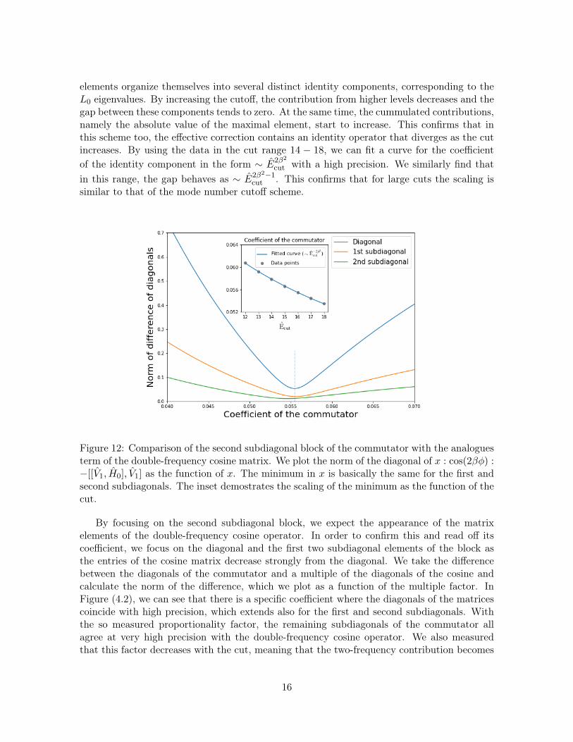
Figure 12: Comparison of the second subdiagonal block of the commutator with the analoguesterm of the double-frequency cosine matrix. We plot the norm of the diagonal of x : cos(2βφ) :−[[V1, H0], V1] as the function of x. The minimum in x is basically the same for the first andsecond subdiagonals. The inset demostrates the scaling of the minimum as the function of thecut.

By focusing on the second subdiagonal block, we expect the appearance of the matrixelements of the double-frequency cosine operator. In order to confirm this and read off itscoefficient, we focus on the diagonal and the first two subdiagonal elements of the block asthe entries of the cosine matrix decrease strongly from the diagonal. We take the differencebetween the diagonals of the commutator and a multiple of the diagonals of the cosine andcalculate the norm of the difference, which we plot as a function of the multiple factor. InFigure (4.2), we can see that there is a specific coefficient where the diagonals of the matricescoincide with high precision, which extends also for the first and second subdiagonals. Withthe so measured proportionality factor, the remaining subdiagonals of the commutator allagree at very high precision with the double-frequency cosine operator. We also measuredthat this factor decreases with the cut, meaning that the two-frequency contribution becomes

16

less and less dominant. Again, we could fit a curve of the form ∼ E−2β2

cut with a very highprecision. We therefore conclude that in the energy cutoff scheme, we find the same operatorsin the effective Hamiltonian as in the oscillator cutoff scheme, and their coefficient also behavessimilarly with the increase of the cut.

Figure 13: Spectrum of the effective Hamiltonian with the false vacuum which confirms thatindeed, the upper unstable equilibrium point turned into an alternate vacuum, just as ithappens in the two-frequency sine-Gordon model. Over this vacuum we can recognize a statewith the same slope, which can be interpreted as a breather-like excitation over the falsevacuum.

All these analyzes convinced us that in the case when we scale λ as Eβ2

cut and considerenergy differences only, we recover the spectrum of the two-frequency model. Indeed usingthe operator Heff with the commutator obtained from the highest cut available, we obtainedthe spectrum on Figure 4.2. This shows without any doubts the presence of the stabilizedupper equilibrium point as a false vacuum. We can also recognize an excited state line parallelwith this vacuum, which can be interpreted as a standing breather-like excitation over thefalse vacuum. This is the quantum analogue of the classical solution, which we demonstratedpreviously.

5 Periodically driven perturbed CFTs

We now extend our analysis from the sine-Gordon model to more general theories. We stillinvestigate theories with Hamiltonians of the form of

H = H0 + V0 + cosωt V1 (26)

but the unperturbed part is assumed to be a generic conformal field theory

H0 =2π

LH0 ; H0 = L0 + L0 −

c

12(27)

17

while the perturbation consists of the integral of relevant spinless (hi = hi) fields, Φ0 and Φ1:

Vi = ci

(L

2π

)1−2hi

Vi ; Vj =

ˆ 2π

0Φj(e

iθ, e−iθ)dθ (28)

The effective Hamiltonian in the ω → ∞ limit takes the generic form (25), which in dimen-sionless quantities reads as

Heff =2π

L

[H1 +

(L

2π

)2−4h1 c21

4[[V1, H1], V1]

](29)

with H1 being the Hamiltonian of the perturbed CFT without the drive

H1 = H0 + c0

(L

2π

)2−2h0

V0 (30)

The details of calculating the commutator is relegated to Appendix (C). In the simplest case,when Φ0 = Φ1, the identity operator always appears in the operator product expansion (OPE)with a diverging term, which can be renormalized by considering energy differences only, justas we did in the sine-Gordon case. Assuming that the OPE starts as

Φ1(z, z)Φ1(0, 0) =1

(zz)2h1+ c2

11

Φ2(0, 0)

(zz)2h1−h2+ . . . (31)

we can scale the amplitude of the drive as c1 ∝ λωEh2−2h1cut , in order to compensate the

dimensions of (zz)h2−2h1 . The effective large frequency Hamiltonian then takes the form

Heff =2π

L

[H0 + c0

(L

2π

)2−2h0

V0 + c2

(L

2π

)2−2h2

V2

](32)

where c2 ∝ λ2 is a scheme-dependent effective coupling. This is the Hamiltonian of a conformalfield theory perturbed by two operators. Thus the periodic drive in the infinite frequencylimit leads to an extra perturbation with an operator, which appears in the OPE of the drivenperturbing operator with itself. These theories could be systematically analyzed with themethods of [18]. Our result can lead to very interesting phenomena and would open a newfield for the Floquet engineering. In particular, in the critical Ising theory, it would imply thatharmonically changing the magnetic field would induce an effective temperature perturbation.

6 Conclusion

In this paper, we investigated the periodically driven sine-Gordon quantum field theory, whichis considered to be the continuum limit of coupled many Kapitza pendula. We focused onthe large frequency behaviour and determined the Floquet quasienergy spectrum for variousdriving protocols. By exploiting the perturbed CFT nature of the sine-Gordon model, wecombined the TCSA method with the usual numerical Floquet analysis in order to get a toolto determine the quasienergy spectrum of the driven sine-Gordon theory for various drivingfrequencies. In the large frequency limit, we compared the results with an analytical calculation

18

based on the large frequency expansion of the effective Hamiltonian. As we found completeagreement, we analyzed the spectrum of this effective Hamiltonian, which is non-trivial andω-independent if we scale the drive with ω. With this driving protocol, we observed a uniformcutoff-dependent shift in the energy spectrum compared to the original sine-Gordon theory.In order to have a non-trivial effect of the drive in energy differences, we had to scale thedrive also with an appropriate power of the energy cutoff. With this protocol, the drivehad a marked effect on the spectrum, which stabilized when we increased the cutoff. Theresulting quasienergy spectrum agreed with the spectrum of the two-frequency sine-Gordontheory. In particular, we observed the signature of another vacuum in the spectrum withhigher bulk energy constant. This other state exists for any volumes, but does not have aninfinite volume limit. It corresponds to the upper equilibrium point of the coupled pendula,which got dynamically stabilized by the periodic drive. We even observed an excitation overthis false vacuum.

In our work we could map the large frequency effective behaviour of the driven systemto another equilibrium system with more parameters and richer dynamics including possiblephase transitions. Similar phenomenon was also analyzed in stochastic driven systems in[19, 20] and our work can be considered its generalization to quantum field theories.

Our investigations and methods can be easily generalized to other periodically drivenconformal field theories. Indeed, we already made the first step into this direction. Wecalculated the effective Hamiltonian in the case when the drive is proportional to ω and anappropriate power of the energy cutoff. In the case when a conformal field theory is perturbedwith a spinless relevant operator, Φ1 via a harmonic time-dependent coupling, the resultingtheory is time independent and has two relevant spinless perturbation, Φ1 and Φ2. The secondperturbation Φ2 corresponds to the first non-trivial operator appearing in the product of Φ1

with itself. In particular, it implies that by perturbing the critical Ising model with a harmonicmagnetic field, the effective theory contains an additional thermal perturbation. It would bevery interesting to explore the consequences of our findings in real systems. Also, assumingthat we harmonically drive a conformal field theory, we can have an effective theory with asingle perturbation, which actually can be integrable. One example is the driven sine-Gordontheory with c0 = 0.

Recently there has been growing interest in periodically driven CFTs [21, 22, 23, 24, 25]. Inthese exactly soluble systems the perturbation is the spatially modulated energy-momentumdensity, which is switched on and off periodically. As a result, the perturbation can be de-scribed in terms of the Virasoro modes and implement conformal transformations, which leavethe system critical. Nevertheless, the stability diagram is extremely rich, which can be studiedvia the evolution of the entanglement entropy. In contrast, in our analysis we focused on thestable large frequency limit of a relevant perturbation. It would very interesting to use similarmethods, such as the investigation of the entanglement entropy and map the stability diagramof our phase space. It would be also very challenging to combine the two type of perturbations.

In the present paper, we were satisfied by establishing that the appropriately scaled, har-monically driven sine-Gordon theory is equivalent to the two-frequency sine-Gordon model.This correspondence, however, can be explored further. Since the two-frequency model has aplenty of interesting phenomena including phase transitions and new states in the spectrum[7, 8, 26], we expect similar behaviour from the driven model, too. As the driven sine-Gordontheory can be realized in cold atom experiments, it would be also very interesting to investigatethe experimental consequences of the appearing two-frequency sine-Gordon model.

19

Acknowledgements

We thank Zoltán Rácz for suggesting the problem and the useful discussions and the NKFIHgrant K134946 for support. The work was supported also by ELKH, while the infrastructurewas provided by the Hungarian Academy of Sciences.

A Large frequency expansion and a numerical approach

Floquet theorem ensures that the solution of the time-dependent Schrödinger equation

i∂Ψ

∂t= HΨ ; H = H0 + V0 + cosωt V1 (33)

has the formψE(φ, t) = e−iEtuE(φ, t) ; uE(φ, t+ T ) = uE(φ, t) (34)

where the quasienergy E governs the slow motion in an effective potential, while the periodicuE is the analogue of the fast modulation. In order to find the effective Hamiltonian, one canmake a periodic gauge transformation [9] of the form

uE(φ, t) = e−iF (t)vE(φ) ; Heff = eiFHe−iF − i(∂teiF )e−iF (35)

where F and Heff can be calculated simultaneously order by order in ω−1:

F = ω−1F1 + ω−2F2 + . . . ; Heff = H(0)eff + ω−1H

(1)eff + ω−2H

(2)eff + . . . (36)

by using that

eiFHe−iF = H + i[F,H]− 1

2[F, [F,H] + . . . ; (∂eiF )e−iF = i∂F − 1

2[F, ∂F ] + . . . (37)

and demanding that Heff is time-independent. At the leading order, the time dependent partof H can be cancelled by F1 as

H(0)eff = H0 + V0 ; F1 = sinωt V1 (38)

At the subleading order, one can ensure H(1)eff = 0 by choosing F2 = −i cosωt [V1, H0 +V0]. At

the next order, F3 can compensate terms only with vanishing average leading to an effectiveterm

H(2)eff =

1

4[[V1, H0 + V0], V1] (39)

In order to test the large frequency approximation in the case of the Kapitza pendulum, wedetermine numerically the Floquet basis, which satisfies the modified Schrödinger equation:

HFuE(φ, t) = EuE(φ, t) ; HF = H − i∂t (40)

Since uE(φ, t) is periodic in time, we simply expand it in Fourier components:

uE(φ, t) =∑m

uE,m(φ)eimωt (41)

20

Figure 14: On the left, there is a plot of the eigenvalues of the Kapitza pendulum obtainedfrom our method. The same eigenvalues appear with shifts of integer multiples of ω, but weonly use the central, so-called fundamental region, which contains all the states with maximalprecision. On the right, there is a plot of the elements of the matrix that diagonalizes the finiteHamiltonian. Its rows correspond to eigenvectors, and one can see that practically, differentblocks contain the same numbers, but they belong to different Fourier modes. These shiftseventually cancel out when one sums up the time-dependent solution, and they result in thesame physical states.

such that the eigenvalue problem takes the form

(mω +H0 + V0)uE,m +1

2V1(uE,m−1 + uE,m+1) = EuE,m (42)

We can further expand uE,m(φ) in the eigenbasis of H0: uE,m(φ) =∑

n cm,n|n〉 which arenothing but the momemtum eigenstates pφ|n〉 = n|n〉, which take the form |n〉 = 1√

2πeinφ.

Since the matrix elements of V0 and V1 are explicitly calculable e±iφ|n〉 = |n±1〉, the eigenvalueproblem reduces to

(mω+n2

2)cm,n+

c0

2(cm,n−1+cm,n+1)+

c1

4(cm−1,n−1+cm+1,n−1+cm−1,n+1+cm+1,n+1) = Ecm,n

(43)Technically, we truncate the tensor product Hilbert space both in m and n to take valuesbetween |m| < mmax and |n| < nmax and diagonalize numerically the finite Hamiltonian. Thequasienergy is defined only modulo ω as we can change E → E ±ω by shifting m. This impliesthat we find any eigenvalue and eigenvector many times. We thus restrict the eigenspectrumby demanding 0 ≤ E < ω, what we call the fundamental region, and order the states wrt. thetime average of the expectation value of the energy 〈H〉 over one driving period.

B TCSA and the driven sine-Gordon model

The quantum version of the periodically driven sine Gordon model is defined by its Hamiltonian(14) with (15). Since φ is an angle variable boundary conditions can be labeled by the integer

21

winding number m as φ(x + L, t) = φ(x, t) + 2πrm, which distinguishes topological sectors.Within each sector we expand the field as

φ(x, t) = 2πmrx

L+

∞∑n=−∞

φn(t)ein2πLx (44)

The zero mode φ0 behaves as a single pendulum. In the free theory its conjugate momentumπ0, satisfying [π0, φ0] = −i, has the spectrum π0|n〉 = n

r |n〉 with periodic wave functions einrφ0

in φ0. The other modes φn can be expanded in terms of creation and annihilation operators.Since the free massless boson is a conformal field theory the field separates into independentleft and right moving parts:

φ(z, z) = ϕ(z) + ϕ(z) ; ϕ(z) =φ0

2− iπ0 log z + i

∑n6=0

anz−n

n(45)

and similarly with z ↔ z and a↔ a for ϕ. Canonical commutation relations imply that

[an, am] = nδn+m ; [an, am] = nδn+m ; [an, am] = 0 (46)

and the Hilbert space is built over the states with given winding and momentum numbers byacting with the left and right moving creation operators (16). The normal ordered Hamiltonianand momentum can be written in terms of the oscillators as in (17). The perturbing operator,having mapped to the plane, takes the form (18), where the normal ordered vertex operator

V β(z, z) =: eiβφ(z,z) := V β0 V

β−V

β+ (47)

can be factorized into the zero mode

V β0 (z, z) = eiβφ0(zz)βπ0 (48)

and the creation-annihilation parts

V β∓ (z, z) =

∏n>0

e±βa∓nz±nn

∏n>0

e±βa∓nz±nn (49)

In calculating the effective Hamiltonian (20) we need to evaluate [[V1, H0], V1], where thedimension-less conformal Hamiltonian is H0 = 2π

L H0 and the dimensionless part of V1 is

V1 =

ˆ 2π

0

dθ

2

(V β(eiθ, e−iθ) + V −β(eiθ, e−iθ)

)(50)

We start to calculate [H0, Vβ(z, z)], with V β(z, z) = V β

0 Vβ−V

β+ . Using the commutation rela-

tions we obtain

[H0, Vβ(z, z)] = [π2

0, Vβ

0 ]V β−V

β+ +

∑n>0

(V β0 [a−nan, V

β− ]V β

+ + V β0 V

β− [a−nan, V

β+ ])

= β(J−(z, z)V β(z, z) + V β(z, z)J+(z, z))

= β2V β(z, z) + (z∂ + z∂)V β(z, z) (51)

22

where we introducedJ∓(z, z) = π0 +

∑n>0

(a∓nz±n + a∓nz

±n) (52)

In calculating the next commutator we obtain

[J∓(z, z), V β(w, w)] = β

(1 +

∑n>0

z±nw∓n +∑n>0

z±nw∓n

)V β(w, w) (53)

In particular, when we calculate the effective Hamiltonian we need terms of the form

[[H0, Vα(z, z)], V β(w, w)] = α[J−(z, z)V α(z, z) + V α(z, z)J+(z, z), V β(w, w)]

= terms multiplying [V α(z, z), V β(w, w)]

+ αβ(∑n

znw−n +∑n

znw−n)V α(z, z)V β(w, w) (54)

Let us note that V α(z, z) =: eiαφ(z,z) :∝ eiαφ(z,z) where the proportionality is a regulatordependent c-number. Since the equal time commutator of φ with itself is vanishing

[φ(x, t), φ(x′, t)] = 0 (55)

the commutator of two vertex operator does not contribute. Furthermore we know the operatorproduct expansion of the vertex operator

V α(z, z)V β(w, w) = (z − w)αβ(z − w)αβ (Vα+β(w, w) + (z − w)∂Vα+β(w, w) + . . . ) (56)

where we indicated the first descendant. Recalling that we have to integrate eventually withz = eiθ, z = e−iθ and w = eiθ

′ and w = e−iθ′ on the unit circle:

ˆ 2π

0

ˆ 2π

0dθdθ′

∑n

ein(θ−θ′)(2− ei(θ−θ′) − e−i(θ−θ′))αβVα+β(eiθ′, e−iθ

′) + . . . (57)

If we would sum up in n from −∞ to ∞ , then we could use that∑

n einθ = 2πδ(θ). This

actually implies that the integral is 0 if αβ > 0 or it is ∞ if αβ < 0. In our case α = ±β andwe always face a divergent behaviour. In order to regularize this we introduce a cutoff in nand analyze the dependence on this cut. The θ integral is periodic and we can evaluate as

ˆ 2π

0dθeinθ(2− 2 cos θ)αβ =

π sec(παβ)Γ(n− αβ)

Γ(−2αβ)Γ(αβ + n+ 1)(58)

It is symmetric in n and the large n behaviour is

Γ(n− αβ)

Γ(αβ + n+ 1)= n−1−2αβ

(1− 1 + 2αβ

n+ . . .

)(59)

This implies that the sum behaves as

nmax∑n=−nmax

Γ(n− αβ)

Γ(αβ + n+ 1)∝ n−2αβ

max (60)

23

We need to analyze two cases. For α = β the sum is convergent and goes to zero. For theleading term in the OPE it goes to zero quite slowly as β2 < 1, however, for descendant theexponent is shifted by an integer, thus it goes to zero much faster. For α = −β the sum isdivergent. For the leading term in the OPE, which contains the identity, it diverges againslowly as β2 < 1. For descendants it is again convergent.

Let us point out that the introduction of the cutoff nmax physically means that we keeponly oscillators, which create particles with conformal energies smaller than nmax. We allowhowever an arbitrary number of these particles showing that the cut is not an energy cut. Inthis regularization scheme the effective Hamiltonian has the structure

H(2)eff ∝

1

4[[V1, H0], V1] ∝ an2β2

maxI + n−2β2

max V2 +O(n−2β2−1max ) (61)

where V2 corresponds to a perturbation with double frequency:

V2 =

ˆ 2π

0dθ

1

2

(V 2β(eiθ, e−iθ) + V −2β(eiθ, e−iθ)

)(62)

Finally, let us develop a numerical method to check these behaviours. The idea is the sameas in the quantum mechanical case. We Fourier expand the periodic Floquet wave functionin time uE(t) =

∑m uE,me

imωt and solve the Floquet eigenvalue problem (14) but now theoperators H0, V0 and V1 act on the conformal Hilbert space. We use the TCSA method torepresent these operators with finite matrices on the truncated Hilbert space. The relevantmatrix element of the perturbation are as follows. The zero mode has matrix elements

〈n,m|V ±β0 |n′,m′〉 = δm,m′δn,n′±1 (63)

while for the sth oscillator we have

〈n,m|alse±βa−s/se∓βas/sak−s|n,m〉 =

k∑i=max(0,k−l)

(k

i

)(−1)isk−i(k − i)!(±β)l−k+2i

(l

k − i

)(64)

These states should be normalized with the square root of 〈0|alsak−s|0〉 = δl,kk!sk. The trun-cated Hilbert space is defined to keep states below a given energy cutoff. Thus this is notequivalent to keep oscillators below a given nmax as even a single oscillator has states witharbitrarily large energies.

Although we were only insterested in the infinite frequency limit, where it is enough todiagonalize the much smaller matrices of the effective theory, our method is applicable togeneral frequencies, where the dynamics can be much more complex. In this case, the time-dependence increases the size of the matrices such that implementing an algorithm that canhandle them can easily become a challenging task.

In our implementation, we used the PRIMME [27, 28] C-package that was specificallydesigned for large-scale eigenvalue problems. PRIMME has an interface that only needs afunction that realizes a matrix-vector multiplication, thus giving the user the complete freedomof representing the matrix. This allows us to exploit the double tensor product structure ofthe Hilbert space so that we only have to store a single block of elements of V0, which reducesthe memory costs to a level that is also sufficient for a general purpose computer.

24

C Calculation of the effective Hamiltonian for generic pertrubedCFTs

In this appendix we calculate the effective Hamiltonian for generic perturbation of CFTs (29).In doing so we recall that

[L0,Φ(z, z)] = hΦ(z, z) + z∂zΦ(z, z) (65)

and similar relations for L0 with z, which are considered to be independent, but put to z = eiθ

and z = e−iθ at the end of the calculation. The standard trick in calculating the equaltime commutator [29] is to exploit the fact that products of operators are well-defined onlywhen they are radially ordered, the analogue of time ordering after the exponential mapping.Thus the commutator can be replaced by radially ordered products, i.e. by deforming the z1

integration around the unit circle C1: a bit increasing the radius in the first and decreasing inthe second term as:˛C1

dz1

˛C1

dz2[Φ1(z1, z2),Φ2(z2, z2)] =

(˛C1+ε

˛C1

−˛C1−ε

˛C1

)dz1dz2R(Φ1(z1, z1),Φ2(z2, z2))

(66)As usual, we do not indicate radial ordering explicitly any more. Radially ordered productshave the operator product expansion (OPE)

Φ1(z1, z1)Φ2(z2, z2) = ci12

1

((z1 − z2)(z1 − z2))h1+h2−hiΦi(z2, z2) + . . . (67)

Since z and z are considered to be independent, not the complex conjugate of each other,when we take |z1| > 1 we have to also take |z1| > 1. This implies that the contributions fromz1 = (1 + ε)eiθ1 , z1 = (1 + ε)e−iθ1 and from z1 = (1 − ε)eiθ1 , z1 = (1 − ε)e−iθ1 cancel eachother. This is not true when we perform the same calculations with z1∂z1Φ1 (or with z1∂z1Φ1)instead of Φ1 as these derivatives introduce an unbalanced pole of the form of 1/(z1 − z2) or1/(z1− z2)). The difference of the integration contours results in a delta function 2πiδ(z1−z2).This is the analogue of the δ(θ1 − θ2) =

∑n e

in(θ1−θ2) term in (57). When calculated withoutan energy cutoff, the delta function puts θ1 to θ2 leading to zero/infinite depending on thesign of h1 + h2 − hi in complete analogy with the similar results in the sine-Gordon theory.In order to get a finite and non-trivial result, we have to scale the amplitude of the drive c1

appropriately with the cutoff.Depending on the rich spectrum of the CFT we can expect numerous interesting cases. In

the following, however, we focus only on the simplest, namely when Φ0 = Φ1. In this case theidentity operator always appears in the OPE with a diverging term, which can be renormalizedby considering energy differences only, just as we did in the sine-Gordon case. Assuming thatthe OPE starts as

Φ1(z, z)Φ1(0, 0) =1

(zz)2h1+ c2

11

Φ2(0, 0)

(zz)2h1−h2+ . . . (68)

we can scale the amplitude of the drive as c1 ∝ λωEh2−2h1cut , in order to compensate the

dimensions of (zz)h2−2h1 . The effective large frequency Hamiltonian then takes the form

Heff =2π

L

[H0 + c0

(L

2π

)2−2h0

V0 + c2

(L

2π

)2−2h2

V2

](69)

25

where c2 ∝ λ2 is a scheme-dependent effective coupling.

References

[1] G. Mussardo, Statistical Field Theory, Oxford Graduate Texts, Oxford University Press,2020.

[2] A. Mitra, Quantum quench dynamics, Annual Review of Condensed Matter Physics 9 (1)(2018) 245–259. doi:10.1146/annurev-conmatphys-031016-025451.

[3] M. Bukov, L. D’Alessio, A. Polkovnikov, Universal high-frequency behavior of periodicallydriven systems: from dynamical stabilization to floquet engineering, Advances in Physics64 (2) (2015) 139–226. doi:10.1080/00018732.2015.1055918.URL http://dx.doi.org/10.1080/00018732.2015.1055918

[4] K. P. L., Dynamic stability of a pendulum when its point of suspension vibrates, SovietPhys. JETP. 21 (1951) 588–597.

[5] R. Citro, E. G. Dalla Torre, L. D’Alessio, A. Polkovnikov, M. Babadi, T. Oka, E. Demler,Dynamical stability of a many-body kapitza pendulum, Annals of Physics 360 (2015)694–710. doi:10.1016/j.aop.2015.03.027.URL http://dx.doi.org/10.1016/j.aop.2015.03.027

[6] V. P. Yurov, A. B. Zamolodchikov, Truncated conformal space approach to scaling Lee-Yang model, Int. J. Mod. Phys. A 5 (1990) 3221–3246. doi:10.1142/S0217751X9000218X.

[7] G. Delfino, G. Mussardo, Nonintegrable aspects of the multifrequency Sine-Gordonmodel, Nucl. Phys. B 516 (1998) 675–703. arXiv:hep-th/9709028, doi:10.1016/S0550-3213(98)00063-7.

[8] Z. Bajnok, L. Palla, G. Takacs, F. Wagner, Nonperturbative study of the two frequencysine-Gordon model, Nucl. Phys. B 601 (2001) 503–538. arXiv:hep-th/0008066, doi:10.1016/S0550-3213(01)00067-0.

[9] S. Rahav, I. Gilary, S. Fishman, Effective hamiltonians for periodically driven systems,Phys. Rev. A 68 (2003) 013820. doi:10.1103/PhysRevA.68.013820.URL https://link.aps.org/doi/10.1103/PhysRevA.68.013820

[10] G. Feverati, F. Ravanini, G. Takacs, Truncated conformal space at c = 1, nonlinearintegral equation and quantization rules for multi - soliton states, Phys. Lett. B 430(1998) 264–273. arXiv:hep-th/9803104, doi:10.1016/S0370-2693(98)00543-7.

[11] L. Samaj, Z. Bajnok, Introduction to the statistical physics of integrable many-bodysystems, Cambridge University Press, Cambridge, 2013.

[12] G. Fodor, P. Forgacs, Z. Horvath, A. Lukacs, Small amplitude quasi-breathers and os-cillons, Phys. Rev. D 78 (2008) 025003. arXiv:0802.3525, doi:10.1103/PhysRevD.78.025003.

26

[13] A. B. Zamolodchikov, Mass scale in the sine-Gordon model and its reductions, Int. J.Mod. Phys. A 10 (1995) 1125–1150. doi:10.1142/S0217751X9500053X.

[14] C. Destri, H. J. de Vega, Nonlinear integral equation and excited states scaling functionsin the sine-Gordon model, Nucl. Phys. B 504 (1997) 621–664. arXiv:hep-th/9701107,doi:10.1016/S0550-3213(97)00468-9.

[15] G. Feverati, F. Ravanini, G. Takacs, Nonlinear integral equation and finite volume spec-trum of Sine-Gordon theory, Nucl. Phys. B 540 (1999) 543–586. arXiv:hep-th/9805117,doi:10.1016/S0550-3213(98)00747-0.

[16] A. B. Zamolodchikov, Two point correlation function in scaling Lee-Yang model, Nucl.Phys. B 348 (1991) 619–641. doi:10.1016/0550-3213(91)90207-E.

[17] G. Delfino, P. Simonetti, J. L. Cardy, Asymptotic factorization of form-factors in two-dimensional quantum field theory, Phys. Lett. B 387 (1996) 327–333. arXiv:hep-th/9607046, doi:10.1016/0370-2693(96)01035-0.

[18] G. Delfino, G. Mussardo, P. Simonetti, Nonintegrable quantum field theories as per-turbations of certain integrable models, Nucl. Phys. B 473 (1996) 469–508. arXiv:hep-th/9603011, doi:10.1016/0550-3213(96)00265-9.

[19] S. B. Dutta, M. Barma, Asymptotic distributions of periodically driven stochastic sys-tems, Physical Review E 67 (6) (Jun 2003). doi:10.1103/physreve.67.061111.URL http://dx.doi.org/10.1103/PhysRevE.67.061111

[20] S. B. Dutta, Phase transitions in periodically driven macroscopic systems, Physical Re-view E 69 (6) (Jun 2004). doi:10.1103/physreve.69.066115.URL http://dx.doi.org/10.1103/PhysRevE.69.066115

[21] X. Wen, J.-Q. Wu, Floquet conformal field theory (2018). arXiv:1805.00031.

[22] R. Fan, Y. Gu, A. Vishwanath, X. Wen, Emergent Spatial Structure and EntanglementLocalization in Floquet Conformal Field Theory, Phys. Rev. X 10 (3) (2020) 031036.arXiv:1908.05289, doi:10.1103/PhysRevX.10.031036.

[23] B. Lapierre, K. Choo, C. Tauber, A. Tiwari, T. Neupert, R. Chitra, Emergent blackhole dynamics in critical Floquet systems, Phys. Rev. Res. 2 (2) (2020) 023085. arXiv:1909.08618, doi:10.1103/PhysRevResearch.2.023085.

[24] B. Lapierre, P. Moosavi, Geometric approach to inhomogeneous Floquet systems, Phys.Rev. B 103 (2021) 224303. arXiv:2010.11268, doi:10.1103/PhysRevB.103.224303.

[25] X. Wen, R. Fan, A. Vishwanath, Y. Gu, Periodically, quasiperiodically, and randomlydriven conformal field theories, Phys. Rev. Res. 3 (2) (2021) 023044. arXiv:2006.10072,doi:10.1103/PhysRevResearch.3.023044.

[26] G. Takacs, F. Wagner, Double sine-Gordon model revisited, Nucl. Phys. B 741 (2006)353–367. arXiv:hep-th/0512265, doi:10.1016/j.nuclphysb.2006.02.004.

27

[27] A. Stathopoulos, J. R. McCombs, PRIMME: PReconditioned Iterative MultiMethodEigensolver: Methods and software description, ACM Transactions on Mathematical Soft-ware 37 (2) (2010) 21:1–21:30.

[28] L. Wu, E. Romero, A. Stathopoulos, Primme_svds: A high-performance preconditionedSVD solver for accurate large-scale computations, SIAM Journal on Scientific Computing39 (5) (2017) S248–S271.

[29] P. H. Ginsparg, Applied Conformal Field Theory, in: Les Houches Summer School inTheoretical Physics: Fields, Strings, Critical Phenomena, 1988. arXiv:hep-th/9108028.

28