Author Proof Chapter 13 Commentary by Zoltán …geza.kzoo.edu/~erdi/cikkek/SomaPeter15.pdfChapter...

UN

CO

RR

EC

TE

D P

RO

OF

Chapter 13Commentary by Zoltán Somogyváriand Péter Érdi

Forward and Backward Modeling: From SingleCells to Neural Population and Back

Zoltán Somogyvári and Péter Érdi

Abstract Some aspects of forward and backward neural modeling are discussed,1

showing, that the neural mass models may provide a “golden midway” between the2

detailed conductance based neuron models and the oversimplified models, dealing3

with the input–output transformations only. Our analysis combines historical per-4

spectives and recent developments concerning neural mass models as a third option5

for modeling large neural populations and inclusion of detailed anatomical data into6

them. The current source density analysis and the geometrical assumption behind7

the different methods, as an inverse modeling tool for determination of the sources8

of the local field potential is discussed, with special attention to the recent results9

about source localization on single neurons. These new applications may pave the10

way to the emergence of a new field of micro-electric imaging.11

13.1 Modeling Population of Neurons: The Third Option12

Structure-based bottom-up modeling has two extreme alternatives, namely13

multi-compartmental simulations, and simulation of networks composed of simple14

elements. There is an obvious trade-off between these two modeling strategies. The15

first method is appropriate to describe the electrogenesis and spatiotemporal propaga-16

Z. Somogyvári (B)Department of Theory, Wigner Research Center for Physics of the HungarianAcademy of Science, Konkoly-Thege Miklós út 29-33, 1121 Budapest, Hungary

Z. SomogyváriDepartment of Epilepsy and General Neurology, National Institute of ClinicalNeurosciences, Budapest, Hungary

Z. Somogyvári · P. ÉrdiCenter for Complex System Studies, Kalamazoo College, 1200 Academy Street,Kalamazoo, Mi 49006, USA

© Springer International Publishing Switzerland 2016R. Kozma and W.J. Freeman, Cognitive Phase Transitions in the CerebralCortex – Enhancing the Neuron Doctrine by Modeling Neural Fields,Studies in Systems, Decision and Control 39, DOI 10.1007/978-3-319-24406-8_13

135

336715_1_En_13_Chapter � TYPESET DISK LE � CP Disp.:8/9/2015 Pages: 147 Layout: T1-Standard

Au

tho

r P

roo

f

UN

CO

RR

EC

TE

D P

RO

OF

136 Z. Somogyvári and P. Érdi

tion of the action potential in single cells, and in small and moderately large networks17

based on data on detailed morphology and kinetics of voltage- and calcium-dependent18

ion channels. The mathematical framework is the celebrated Hodgkin–Huxley model19

[19] supplemented with the cable theory [34, 35]. The construction of neural simula-20

tion softwares such as NEURON [17, 18], and GENESIS [5] contributed very much21

to make the emerging field of computational neuroscience is able to make realistic22

bottom up neural simulations. The second approach grew up from the combination of23

the McCulloch–Pitt neuron models and the of the Hebbian learning rule, and offers a24

computationally efficient method for simulating large network of neurons where the25

details of single cell properties are neglected. A classical example of using two-level26

neural network models by combining activity and synaptic dynamics as a model of27

generating ordered neural pattern by a self-organizing algorithm is [47], and a newer28

one for invariant pattern recognitions in the same spirit [4].29

As concerns single cell modeling, there is a series of cell models with different30

level of abstraction. While multi-compartmental models take into account the spatial31

structure of a neuron, neural network techniques are generally based on integrate-32

and-fire models. The latter is a spatially homogeneous, spike-generating device. For33

a review of ‘spiking neurons’ see [13]. As is well known, neural network theory,34

incorporating biologically non-plausible learning rules became a celebrated sub-35

class of machine learning discipline called artificial neural network. Modeling pop-36

ulation of neurons emerged as a compromise between “too microscopic” and “too37

macroscopic” descriptions [10].38

13.2 Mesoscopic Neurodynamics39

13.2.1 Statistical Neurodynamics: Historical Remarks40

There is a long tradition to try to connect the ‘microscopic’ single cell behavior to41

the global ‘macrostate’ of the nervous system analogously to the procedures applied42

in statistical physics. Global brain dynamics is handled by using continuous (neural43

field) description instead of the networks of discrete nerve cells. Both deterministic,44

field-theoretic [1, 15, 37, 46] and more statistical approaches have been developed.45

[10] introduced a modular and therefore hierarchical framework of neural field mod-46

els, as the series of K models from K0 to KIII. This series of more and more complex47

neural mass models has been reached the level of behavioral analysis with the KIII48

sets. Later, [25] extended the K sets theory to the next (KIV) level to account for49

the interaction between cortical areas as well. One of us (PE) participated in the50

application of KIV system for hippocampus-related problems [26, 27].51

This way, the otherwise pure statistical handling of neural populations gains new52

anatomical details.53

54


Au

tho

r P

roo

f

UN

CO

RR

EC

TE

D P

RO

OF

13 Commentary by Zoltan Somogyvari and PeterErdi 137

Francesco Ventriglia constructed a neural kinetic theory of large-scale brain55

activities that he presented in a series of somewhat overlooked papers [41–44]. His56

statistical theory is based on two entities: spatially fixed neurons and spatially propa-57

gating impulses. Neurons might be excitatory or inhibitory and their states are char-58

acterized by their subthreshold membrane potential or inner excitation, threshold59

level for firing, a resting level of inactivity state, maximum hyperpolarization level,60

absolute refractoriness period and a synaptic delay time. Under some conditions they61

emit impulses. Neurons are grouped in populations, state of the neurons in the pop-62

ulation is described by the population’s probability density function. Impulses move63

freely in space (in the numerical implementation some rule should be defined due64

to treat the effects due to spatial discretization), and might be absorbed by neurons65

chaining their inner excitation. Impulses are distributed in velocity–space according66

to the corresponding probability density function.67

We extended [2, 16] this theory by using diffusion theory in two different senses.68

Both the dynamical behavior of neurons in their state-space and the movement of69

spikes in the physical space have been considered as diffusion processes. The state-70

space in the model consists of the two-dimensional space coordinate r for both71

neurons and spikes, a membrane potential coordinate u for all types of neurons, and72

an intracellular calcium-concentration coordinate χ for pyramidal neurons only. Both73

cell types, the inhibitory and excitatory ones are described by ionic conductances74

specific to neuronal type. Instead of fixed firing threshold a soft firing threshold is real-75

ized by voltage-dependent firing probability. Absorbed spikes induce time-dependent76

postsynaptic conductance change in neurons, expressed by the alpha-function.77

78

We also realized in Budapest the importance of the existence of the database79

on connectivity in the cat cerebral cortex published in 1995, [36] and the necessity80

to include time delays. While our simulations of the activity propagation in hip-81

pocampus slices was based on the usual statistical assumptions, the first simulations82

by incorporating real connectivity data was done (well, with some time delay) by83

Tamás Kiss [23]. We (he) also took into account the axonal time delay. To calculate84

the the synaptic current a new term εs(r, u,χ, t) has been added:85

γs′s = γolds′s + γ′

s′sτ ′

s′s

∞∫

0

dt ′∫

�(r′)

κ(r, r′) · as′s(r, t − td − t ′) · t ′ · exp

(1 − t ′

τ ′s′s

),

(13.1)

86

87

where the κ(r, r′) function determines the source and target cortical area between88

which information exchange occurs. Activity produced by the source population89

influences the target population after td time delay giving account of signal propa-90

gation delay in fibers.91

The method and results were published in his master thesis written in Hungarian92

[23], (not necessarily the best marketing strategy). We made early not well-published93


Au

tho

r P

roo

f

UN

CO

RR

EC

TE

D P

RO

OF


(it is our fault) studies also on the disconnection syndromes, and simulated what it94

is now called connectopathy [8].95

Statistical neurodynamics has at least two different features, as statistical mechan-96

ics. First, in neurodynamics “mean-field” approach is not enough, we should see both97

global and local dynamics. Our model gave the possibility to simulate the statistical98

behavior of large neural populations, and synchronously to monitor the behavior of99

an average single cell. Second, both statistical and specific cortical connections exist,100

model frameworks should describe their combination. In the project described in our101

last paper in the topic [24] both features were incorporated. As it was already written102

in [9], p. 272: “I think, each research group has bedroom secrets. The story with our103

“population model” is ours, and I think I should not blab it out.”104

Viktor Jirsa [20] classified the mesoscopic models into the following categories:105

• Infinite Propagation Speed,Arbitrary Connectivity106

• Finite Propagation Speed,Arbitrary Connectivity107

• Infinite Propagation Speed, Symmetric, and Translationally Invariant Connectivity108

• Infinite Propagation Speed, Symmetric and Translationally Variant Connectivity109

• Finite Propagation Speed, Symmetric, and Translationally Invariant Connectivity110

• Finite Propagation Speed,Asymmetric and Translationally Variant Connectivity111

A general framework for neural field models with local and global connections also112

with time delay was given by him [21]. This model framework became the scientific113

basis of the Virtual Brain Project [45].114

13.3 Forward and Inverse Modeling of the Neuro-Electric115

Phenomena116

As we have seen in the previous paragraphs, that a strong branch of the modeling117

tradition in the neuroscience follows the bottom-up approach on the tracks of Hodgkin118

and Huxley. Starting from the biophysical mechanisms of the ion channels one can119

built neuron models on arbitrary levels of complexity. Then, connecting the neurons120

into networks, implementing connections from the basic synaptic dynamics up to the121

advanced activity dependent learning methods, one can study the emerging network122

dynamics. In the next step, as we will see here, solving the forward problem of the123

Poisson-equation, an artificial LFP can be synthesized and compared to the observed124

phenomena during electrophysiological measurements.125

While the role of the modeling is less obvious in the top-down approach, it will126

be shown in this section, that models and modeling have an indispensable role, when127

we want to understand the measured electric signals by decomposing them into their128

sources. Here the model means a set of constrains and prior assumptions about the129

sources which implicitly or explicitly adopted by each method, to find a unique130

solution to source determination problem.131


Au

tho

r P

roo

f

UN

CO

RR

EC

TE

D P

RO

OF


13.3.1 Micro-Electric Imaging132

An average neuron in the cortex receives 10–15 thousand synapses from other neu-133

rons. While many fine details are known about the properties of individual synapses,134

and there is a progress on understanding brain connectivity [40], the spatio-temporal135

transmembrane current patterns, resulting from the summation of a huge number136

of individual synaptic inputs on a whole neuron, are almost entirely unknown. The137

main reason for this large gap in our knowledge is the lack of a proper technique for138

measuring spatio-temporal inputs patterns on single neurons in behaving animals.139

While the output of a neuron is well recognizable in the extracellular potential mea-140

surements in the form of action potentials, the input that evoked the observed spike is141

unknown. Without knowing the input, deciphering the input–output transformation142

implemented by an individual neuron is hopeless.143

The steadily improving optical imaging techniques provide extremely good spa-144

tial resolution, but they still have not reached the speed, signal-to-noise ratio, sam-145

pling frequency, aperture and miniaturization properties necessary to record action146

potentials and synaptic input patterns on whole neurons in behaving animals.147

On the other hand, the number of channels, together with the spatial resolu-148

tion, have dramatically increased recently in the widely used multi-electrode arrays149

(MEA), and further improvements are expected [3, 6, 22]. This relatively low cost150

technique is applicable to freely behaving animals as well. Traditionally, only the151

spike timings are used from these extracellular (EC) potential recordings, but recent152

improvements significantly increased the spatial information content of these mea-153

surements. Thus, new techniques of data analysis are needed to exploit this new154

information.155

We conclude that the rapid development of MEA techniques and the set of new156

analysis methods, directly designed to exploit the spatial information content of MEA157

recordings, may help to create a new emerging field to be called micro-electric158

imaging. Similar to the macroscopic imaging techniques, the different tasks of this159

field are: forward modeling, source reconstruction, anatomical area and layer deter-160

mination, correlation and causality analysis while a specific task on this microscopic161

field is membrane potential and synaptic current reconstruction.162

During the last few decades, a large variety of mathematical source reconstruc-163

tion algorithms or imaging techniques have been developed for macroscopic neural164

electro-magnetic measurements, such as EEG and MEG. For a review, see [14].165

However, on micro scales, only the traditional current source density (CSD) method166

has served the aim of identifying the neural transmembrane sources underlying167

the observed EC potential [30, 31]. The traditional CSD works well if the full 3-168

dimensional potential distribution is known with the spatial resolution comparable169

to the size of the sources. Definitely, current sources on single neurons cannot be ana-170

lyzed this way, since 3D data cannot be collected by electrode systems without large171

tissue damage. Lacking this full 3D data, the CSD analysis based on 2D and 1D MEA172

measurements intrinsically requires the adoption of assumptions about homogeneity173

of the source density in the unknown dimensions. This homogeneity assumption can174


Au

tho

r P

roo

f

UN

CO

RR

EC

TE

D P

RO

OF


be a good approximation in the case of large population activities, but it is certainly175

not valid for single cell sources. Thus, we can conclude, that the (implicit) source176

model of the traditional 1D CSD analysis is an infinite homogeneous laminar source.177

13.3.2 Source Reconstruction on Single Neurons178

An alternative approach for CSD estimation is based on the inverse of the forward179

solution. To our knowledge, the first inverse CSD method was developed and applied180

to LFP data of olfactory bulb by Walter J. Freeman in 1980 [11, 12]. The inverse181

method was not applied to LFP data since, till it was rediscovered in recent years and182

applied to extracellular action potentials by [38] and local field potentials by [32].183

The first inverse method for the estimation of cell-electrode distance and the184

reconstruction of the CSD on single neurons was introduced in our own lab [38] in185

2005. The source model applied here called counter current model was a line-source,186

parallel to the electrode and consists of one high negative (sink) current peak on a187

smooth background of positive counter currents (sources). This model is valid only188

until the negative peak of the extracellular spike, so this single cell CSD method189

is able to calculate the CSD only at the peak of the action potential. Since then,190

numerous inverse CSD methods have been developed in many other research groups191

as well. Pettersen et al. [32] developed inverse CSD solutions for LFP, generated by192

a cortical column. The corresponding source model consists of homogeneous discs,193

whose laminar distribution was described either as sum of thin discs or a spline194

interpolated continuous distribution. Later, Daniel Wójcik and his group used kernel195

methods for 1, 2 and 3D inverse solutions [28, 29, 33]. The source models here196

consist of 3D Gaussian blobs and ensures a smooth inverse solution.197

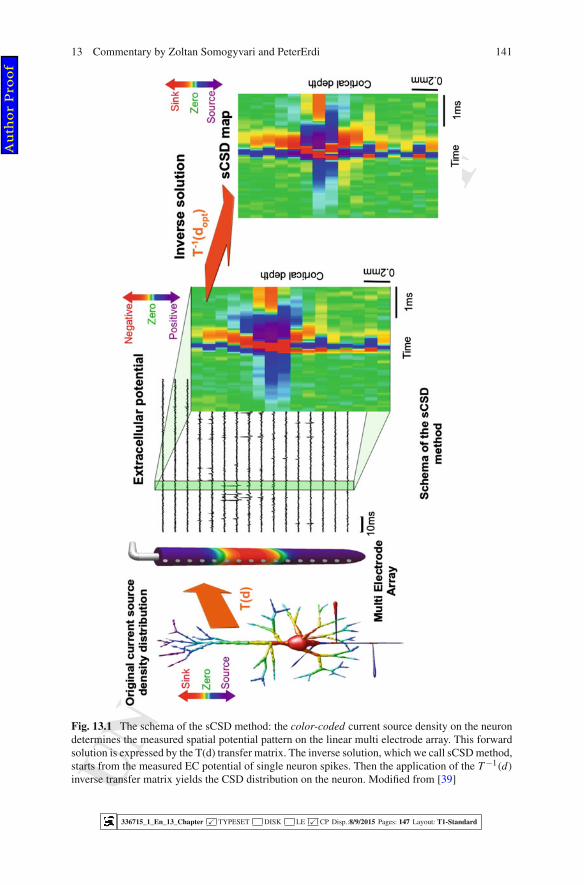
The recent sCSD method [39], built on the basis of the counter current model, is198

able to reconstruct the full spatio-temporal CSD dynamics of single neurons during199

the action potentials. By the sCSD method, the EC observability of back propagating200

action potentials in the basal dendrites of cortical neurons, the forward propagation201

preceding the action potential on the dendritic tree and the signs of the Ranvier-nodes202

has been demonstrated for the first time (Fig. 13.1).203

13.3.3 Anatomical Area and Layer Determination:204

Micro-Electroanatomy205

Proper interpretation of single neuron CSD maps during in vivo application of MEAs206

requires precise identification of the anatomical structures, cortical and synaptic207

layers in which the EC potentials were recorded. Post-hoc histology can provide208

information on the position of the probes in the brain, but it would be advantageous209

if this information would be accessible during the experiment as well, and in some210


Au

tho

r P

roo

f

UN

CO

RR

EC

TE

D P

RO

OF


Fig. 13.1 The schema of the sCSD method: the color-coded current source density on the neurondetermines the measured spatial potential pattern on the linear multi electrode array. This forwardsolution is expressed by the T(d) transfer matrix. The inverse solution, which we call sCSD method,starts from the measured EC potential of single neuron spikes. Then the application of the T −1(d)

inverse transfer matrix yields the CSD distribution on the neuron. Modified from [39]


Au

tho

r P

roo

f

UN

CO

RR

EC

TE

D P

RO

OF


Fig. 13.2 Electroanatomy of the hippocampus. Somatic and synaptic layers are determined solelybased on the recorded data. a Somatic layers were identified based on a high frequency (300Hz) power map. b Synaptic layers were determined by coherence-based clustering. c The bor-ders between layers and areas of the hippocampus is inferred by fusing the somatic map with thecoherence-clusters. Our coherence-tracking algorithm visualizes the hippocampal anatomical struc-ture clearly. d Comparison with histology. Arrows mark the paths of the 8 shanks of the electrode.From [3]


Au

tho

r P

roo

f

UN

CO

RR

EC

TE

D P

RO

OF


Fig. 13.3 Demonstration of different input patterns onto the same neuron. The same neuron(denoted by a star) is activated by different pathways and emits action potentials during thetaand sharp-wave ripple oscillations. (Work of Z. Somogyvri and A. Bernyi, from [7], Fig. 6)

cases the post-hoc histology cannot be performed well. The methodology of micro-211

electroanatomy [3], which was able to determine and visualize anatomical structures212

and synaptic layers in the hippocampus and in the neocortex solely based on the213

recorded multi-channel LFP data was a recent attempt on that. This anatomical214

reconstruction serves as a good basis for investigation of different synaptic input215

pathways on the neurons (Fig. 13.2).216

Our preliminary results, previewed in the Nature Reviews Neuroscience [7] have217

provided a new insight into hippocampal dynamics, showing that the same CA1218

interneuron receives input on different pathways in different hippocampal states.219

More precisely, the input was found to be dominated by the entorhinal perforant path220

during theta oscillations, but the Schaffer-collateral input from CA3 was stronger dur-221

ing sharp-wave ripple (SPW-R) periods. Thus, we conclude, that new, high-channel-222

count MEA data, precise identification of synaptic layers and model-based source223

reconstruction technique make possible a systematic analysis of synaptic input pat-224

terns for different cell types in different subregions of the hippocampus (Fig. 13.3).225

13.4 Conclusions226

We reviewed some specific concepts, where density functions play important role227

and may provide novel approaches for inferring, modeling and understanding neural228

dynamics and functions. In the first section we have briefly reviewed the application229

of density functions in the neural mass models as a ‘golden midway’ between to too230

detailed microscopic and the too phenomenological macroscopic approaches. This231

historical point of view led us to the conclusion, that the anatomical knowledge on232

the brain connectivity structure should be included into the pure statistical treatment233

as well. Besides some early attempts for our own laboratory, we recognized a strong234

trend into this direction in the recent years.235


Au

tho

r P

roo

f

UN

CO

RR

EC

TE

D P

RO

OF


On the other side, density functions have inevitable role in the inference of the236

neural currents from the extracellular potential measurements, known as current237

source density analysis. In the CSD analysis, the collective effect of the abundant238

number of individual synapses is described by an appropriate density function. We239

have shown, that the solution of this inverse problem depends on the geometrical240

and dynamical assumptions about the sources. Different CSD methods use different241

source models, defining their range of validity and applicability. Finally we showed,242

that a new and promising branch of CSD methods emerged as the density functions243

have been applied to single neurons, allowing the inference of input current source244

density patterns on single neurons.245

Acknowledgments ZS was supported by grant OTKA K 113147. PE thanks to the Henry Luce246

Foundation to let him to be a Henry R Luce Professor.247

References248

1. Amari S (1983) Field theory of self-organizing neural nets. IEEE Trans Syst Man Cybern249

SMC–13:741–748250

2. Barna Gy, Grobler T, Érdi P (1988) Statistical model of the Hippocampal CA3 region I. The251

single-cell module: bursting model of the pyramidal cell. Biol Cybern 79:301–308252

3. Berényi A, Somogyvári Z, Nagy A, Roux L, Long J, Fujisawa S, Stark E, Leonardo A, Harris253

T, Buzski G (2014) Large-scale, high-density (up to 512 channels) recording of local circuits254

in behaving animals. J. Neurophysiol 111:1132–1149. doi:10.1152/jn.00785.2013BiolCybern,255

79:309-321256

4. Bergmann U, von der Malsburg C (2011) Self-organization of topographic bilinear networks257

for invariant recognition. Neural Comput 23:2770–2797258

5. Bower JM, Beeman D (1994) The book of GENESIS: exploring realistic neural models with259

the GEneral NEural SImulation System. TELOS, Springer, New York260

6. Buzsáki G (2004) Large-scale recording of neuronal ensembles. Nat Neurosci 7(5):446–51261

7. Buzsáki G, Anastassiou CA, Koch C (2012) The origin of extracellular fields and currents–262

EEG, ECoG, LFP and spikes. Nat Rev Neurosci 13(6):407–420263

8. Érdi P (2000) Narrowing the gap between neural models and brain imaging data: a mesoscopic264

approach to neural population dynamics. The 2000 Neuroscan Workshop at Duke University.265

http://www.rmki.kfki.hu/biofiz/cneuro/tutorials/duke/index.html266

9. Érdi P (2007) Complexity explained. Springer, New York267

10. Freeman WJ (1975) Mass action in the nervous system. Academic Press, Massachusetts268

11. Freeman WJ (1980) A software lens for image reconstitution of the EEG. Prog Brain Res269

54:123–127270

12. Freeman WJ (1980) Use of spatial deconvolution to compensate for distortion of EEG by271

volume conduction. IEEE Trans Biomed Eng 27(8):421–429272

13. Gerstner W, Kistler M, Naud R, Paninski (2014) Neuronal dynamics: from single neurons to273

networks and models of cognition. Cambridge University Press, Cambridge274

14. Grech R, Cassar T, Muscat J, Camilleri KP, Fabri GS, Zervakis M, Xanthopoulos P, Sakkalis275

V, Vanrumste B (2008) Review on solving the inverse problem in EEG source analysis. J276

NeuroEng Rehabil 5(25):1–33277

15. Griffith JA (1963) A field theory of neural nets. I. Derivation of field equations. Bull Math278

Biophys 25:111–120279

16. Grobler T, Barna Gy, Érdi P (1998) Statistical model of the Hippocampal CA3 region II. The280

population framework: model of rhythmic activity in the CA3 slice. Biol Cybern 79:309–321281


Au

tho

r P

roo

f

http://dx.doi.org/10.1152/jn.00785.2013BiolCybern,79:309-321

http://dx.doi.org/10.1152/jn.00785.2013BiolCybern,79:309-321

http://www.rmki.kfki.hu/biofiz/cneuro/tutorials/duke/index.html

UN

CO

RR

EC

TE

D P

RO

OF


17. Hines M (1984) Efficient computation of branched nerve equations. J Biol-Med Comp 15:69–282

74283

18. Hines M (1993) The NEURON simulation program. Neural network simulation environments.284

Kluwer Academic Publication, Norwell285

19. Hodgkin A, Huxley A (1952) A quantitative description of membrane current and its application286

to conduction and excitation in nerve. J Physiol 117:500–544287

20. Jirsa VK (2004) Connectivity and dynamics of neural information processing. Neuroinformat-288

ics 2:183204289

21. Jirsa V,K (2009) Neural field dynamics with local and global connectivity and time delay.290

Philos Trans R Soc A: Math Phys Eng Sci 367(1891):1131–1143291

22. Kipke D, Shain W, Buzsáki G, Fetz E, Henderson J, Hetke J, Schalk G (2008) Advanced292

neurotechnologies for chronic neural interfaces: new horizons and clinical opportunities. J293

Neurosci 28(46):11830–11838294

23. Kiss T (2000) Az agykéreg normális és epileptikus muködésének tanulmányozása statisztikus295

neurodinamikai modellel (in Hungarian). Master’s thesis, Eötvös Lorán Tudományegyetem.296

http://cneuro.rmki.kfki.hu/files/diploma.pdf297

24. Kiss T, Érdi P (2002) Mesoscopic Neurodynamics. BioSystems, Michael Conrad’s special298

issue 64(1–3):119–126299

25. Kozma R, Freeman WJ (2003) Basic principles of the KIV model and its application to the300

navigation problem. J Integr Neurosci 2(1):125–145301

26. Kozma R, Freeman WJ, Érdi P (2003) The KIV model—nonlinear spatio-temporal dynamics302

of the primordial vertberate forebrain. Neurocomputing 52–54:819–826303

27. Kozma R, Freeman WJ, Wong D, Érdi P (2004) Learning environmental clues in the KIV304

model of the Cortico-Hippocampal formation. Neurocomputing 58–60(2004):721–728305

28. Leski S, Wajcik DK, Tereszczuk J, Awiejkowski DA, Kublik E, Wrabel A (2007) Inverse306

Current-Source Density in three dimensions. Neuroinformatics 5:207307

29. Leski S, Pettersen KH, Tunstall B, Einevoll GT, Gigg J, Wajcik DK (2011) Inverse Current308

Source Density method in two dimensions: inferring neural activation from multielectrode309

recordings. Neuroinformatics 9:401–425310

30. Mitzdorf U (1985) Current source-density method and application in cat cerebral cortex: inves-311

tigation of ecoked potentials and EEG phenomena. Physiol Rev 65:37–100312

31. Nicholson C, Freeman JA (1975) Theory of current source-density analysis and determination313

of conductivity tensor for anuran cerebellum. J Neurophysiol 38:356–368314

32. Pettersen KH, Devor A, Ulbert I, Dale AM, Einevoll GT (2006) Current-source density esti-315

mation based on inversion of electrostatic forward solution: effect of finite extent of neuronal316

activity and conductivity discontinuites. J Neurosci Methods 154(1–2):116–133317

33. Potworowski J, Jakuczun W, eski S, Wjcik DK (2012) Kernel current source density method.318

Neural Comput 24:541–575319

34. Rall W (1962) Electrophysiology of a dendritic neuron model. Biophys J 2:145–167320

35. Rall W (1977) Core conductor theory ad cable properties of neurons. Handbook of physiology.321

The nervous system. William and Wilkins, Baltimore, pp 39–98322

36. Scannell JW, Blakemore C, Young MP (1995) J Neurosci 15:1463–1483323

37. Seelen W (1968) Informationsverarbeitung in homogenen netzen von neuronenmodellen.324

Kybernetik 5:181–194325

38. Somogyvári Z, Zalányi L, Ulbert I, Érdi P (2005) Model-based source localization of extracel-326

lular action potentials. J Neurosci Methods 147:126–137327

39. Somogyvári Z, Cserpán D, Ulbert I, Érdi P (2012) Localization of single-cell current sources328

based on extracellular potential patterns: the spike CSD method. Eur J Neurosci 36(10):3299–329

313330

40. Sporns O (2010) Networks of the brain. MIT Press, Cambridge331

41. Ventriglia F (1974) Kinetic approach to neural systems. Bull Math Biol 36:534–544332

42. Ventriglia F (1982) Kinetic theory of neural systems: memory effects. In: Trappl R (ed) Proceed-333

ings of the Sixth European Meeting on Cybernetics and Systems Research. Austrian Society334

for Cybernetic Studies, North-Holland Publishing Company, Amsterdam, pp 271–276335


Au

tho

r P

roo

f

http://cneuro.rmki.kfki.hu/files/diploma.pdf

UN

CO

RR

EC

TE

D P

RO

OF


43. Ventriglia F (1990) Activity in cortical-like neural systems: short-range effects and attention336

phenomena. Bull Math Biol 52:397–429337

44. Ventriglia F (1994) Towards a kinetic theory of cortical-like neural fields. Neural modeling and338

neural networks. Pergamon Press, Oxford, pp 217–249339

45. The Virtual Brain Project. http://www.thevirtualbrain.org/tvb/zwei340

46. Wilson HR, Cowan J (1973) A mathematical theory of the functional dynamics of cortical and341

thalamic neurons tissue. Kybernetik 13:55–80342

47. Willshaw DJ, von der Malsburg C (1976) How patterned neural connections can be set up by343

self-organization. Proc R Soc Lond B194:431–445344


Au

tho

r P

roo

f

http://www.thevirtualbrain.org/tvb/zwei

UN

CO

RR

EC

TE

D P

RO

OF

Author Queries

Chapter 13

Query Refs. Details Required Author’s response

No queries.

Au

tho

r P

roo

f

Author Proof Chapter 13 Commentary by Zoltán …geza.kzoo.edu/~erdi/cikkek/SomaPeter15.pdfChapter...

Documents

Transcript of Author Proof Chapter 13 Commentary by Zoltán …geza.kzoo.edu/~erdi/cikkek/SomaPeter15.pdfChapter...