University of Kentucky University of Kentucky

UKnowledge UKnowledge

Theses and Dissertations--Physics and Astronomy Physics and Astronomy

2012

ZEEMAN EFFECT STUDIES OF MAGNETIC FIELDS IN THE MILKY ZEEMAN EFFECT STUDIES OF MAGNETIC FIELDS IN THE MILKY

WAY WAY

Kristen Lynn Thompson University of Kentucky, klthompson9@gmail.com

Right click to open a feedback form in a new tab to let us know how this document benefits you. Right click to open a feedback form in a new tab to let us know how this document benefits you.

Recommended Citation Recommended Citation Thompson, Kristen Lynn, "ZEEMAN EFFECT STUDIES OF MAGNETIC FIELDS IN THE MILKY WAY" (2012). Theses and Dissertations--Physics and Astronomy. 12. https://uknowledge.uky.edu/physastron_etds/12

This Doctoral Dissertation is brought to you for free and open access by the Physics and Astronomy at UKnowledge. It has been accepted for inclusion in Theses and Dissertations--Physics and Astronomy by an authorized administrator of UKnowledge. For more information, please contact UKnowledge@lsv.uky.edu.

STUDENT AGREEMENT: STUDENT AGREEMENT:

I represent that my thesis or dissertation and abstract are my original work. Proper attribution

has been given to all outside sources. I understand that I am solely responsible for obtaining

any needed copyright permissions. I have obtained and attached hereto needed written

permission statements(s) from the owner(s) of each third-party copyrighted matter to be

included in my work, allowing electronic distribution (if such use is not permitted by the fair use

doctrine).

I hereby grant to The University of Kentucky and its agents the non-exclusive license to archive

and make accessible my work in whole or in part in all forms of media, now or hereafter known.

I agree that the document mentioned above may be made available immediately for worldwide

access unless a preapproved embargo applies.

I retain all other ownership rights to the copyright of my work. I also retain the right to use in

future works (such as articles or books) all or part of my work. I understand that I am free to

register the copyright to my work.

REVIEW, APPROVAL AND ACCEPTANCE REVIEW, APPROVAL AND ACCEPTANCE

The document mentioned above has been reviewed and accepted by the student’s advisor, on

behalf of the advisory committee, and by the Director of Graduate Studies (DGS), on behalf of

the program; we verify that this is the final, approved version of the student’s dissertation

including all changes required by the advisory committee. The undersigned agree to abide by

the statements above.

Kristen Lynn Thompson, Student

Dr. Thomas H. Troland, Major Professor

Dr. Tim Gorringe, Director of Graduate Studies

ZEEMAN EFFECT STUDIES OF MAGNETIC FIELDS IN THE MILKY WAY

DISSERTATION

A dissertation submitted in partialfulfillment of the requirements forthe degree of Doctor of Philosophyin the College of Arts and Sciences

at the University of Kentucky

ByKristen Lynn Thompson

Lexington, Kentucky

Director: Thomas H. Troland, Professor of Physics and AstronomyLexington, Kentucky 2012

Copyright c© Kristen Lynn Thompson 2012

ABSTRACT OF DISSERTATION

ZEEMAN EFFECT STUDIES OF MAGNETIC FIELDS IN THE MILKY WAY

The interstellar medium (ISM) of our Galaxy, and of others, is pervaded by ultralow-density gas and dust, as well as magnetic fields. Embedded magnetic fields havebeen known to play an important role in the structure and dynamics of the ISM.However, the ability to accurately quantify these fields has plagued astronomers formany decades. Unfortunately, the experimental techniques for measuring the strengthand direction of magnetic fields are few, and they are observationally challenging. Theonly direct method of measuring the magnetic field is through the Zeeman effect.

The goal of this dissertation is to expand upon the current observational studiesand understanding of the effects of interstellar magnetic fields across various regionsof the Galaxy. Zeeman effect observations of magnetic fields in two dynamicallydiverse environments in the Milky Way are presented: (1) An OH and HI absorptionline study of envelopes of molecular clouds distributed throughout the Galaxy, and(2) A study of OH absorption lines toward the Galactic center region in the vicinityof the supermassive black hole Sgr A*.

We have executed the first systematic observational survey designed to determinethe role of magnetic fields in the inter-core regions of molecular clouds. Observationsof extragalactic continuum sources that lie along the line-of-sight passing throughGalactic molecular clouds were studied using the Arecibo telescope. OH Zeemaneffect observations were combined with estimates of column density to allow for com-putation of the mass-to-flux ratio, a measurement of the gravitational to magneticenergies within a cloud. We find that molecular clouds are slightly subcritical overall.However, individual measurements yield the first evidence for magnetically subcriticalmolecular gas.

Jansky VLA observations of 18 cm OH absorption lines were used to determinethe strength of the line-of-sight magnetic field in the Galactic center region. Thisstudy yields no clear detections of the magnetic field and results that differ from asimilar study by Killeen, Lo, & Crutcher (1992). Our results suggest magnetic fields

no more than a few microgauss in strength.

KEYWORDS: Galactic Center, Magnetic Fields, MolecularClouds, Interstellar Medium, Zeeman Effect

Author:Kristen Lynn Thompson

Date: December 7, 2012

ZEEMAN EFFECT STUDIES OF MAGNETIC FIELDS IN THE MILKY WAY

By

Kristen Lynn Thompson

Thomas H. Troland

Director of Dissertation

Tim Gorringe

Director of Graduate Studies

December 7, 2012

Date

To my family, who have always supported and encouraged me to pursue my dreams.

ACKNOWLEDGMENTS

When attempting to remember all the people who have helped you get to where youare today, one quickly realizes that there are far too many individuals to mention. Iwould like to thank my parents, John and Brenda Thomas, for all their love, support,and encouragement. They taught me that “You can achieve whatever you put yourmind to,” and I’ve grown to realize that those are some motivating words to liveby. I would like to thank my husband, Grant Thompson, for supporting me day andnight, and for providing me with endless encouragement to help me get through boththe good and the bad times. Thank you to my grandparents Lonie and Jean AnnCronin, and the rest of my family, for always believing in me and being patient whileI seemingly pursued the career of professional student.

I will forever be indebted to my thesis advisor, Dr. Tom Troland, for giving me theopportunity to come to UK and pursue my dreams. He believed in me from the daywe had a chance meeting in Green Bank, West Virginia, and without him, there aremany things in my life that would be much different. Thank you, also, to the restof my thesis committee, Dr. Gary Ferland, Dr. Wolfgang Korsch, and Dr. FrankEttensohn for all of their insight. I would also like to thank Carl Heiles at Berkeley forhis help with all the details of observing with the Arecibo telescope and subsequentdata reduction. I also acknowledge help from Richard Crutcher at the University ofIllinois for his insight on our mass-to-flux ratio results.

I want to thank all of the friends who adopted me when I arrived at UK and who havehelped me maintain my sanity along the way. We have spent many hours gatheredaround a kitchen table doing countless physics problems together, and I’m certainthat Jackson E&M would have been the death of me if not for my wonderful groupof friends. Ben, Emily, Erin, and Gretchen - you are a wonderful support team, andthanks for everything!

Last, but certainly not least, a big thanks goes out to my grandparents, Bill andIrmgard Thomas. Nana and Pap, I wish you were here to share this moment withme, but I know that there are holes in the floor of Heaven and you have been myguardian angels seeing me through this whole process. This one’s for you.

iii

TABLE OF CONTENTS

Acknowledgments . . . . . . . . . . . . . . . . . . . . . . . . . . . . . . . . . iii

Table of Contents . . . . . . . . . . . . . . . . . . . . . . . . . . . . . . . . . iv

List of Tables . . . . . . . . . . . . . . . . . . . . . . . . . . . . . . . . . . . . vi

List of Figures . . . . . . . . . . . . . . . . . . . . . . . . . . . . . . . . . . . vii

Chapter 1 Introduction . . . . . . . . . . . . . . . . . . . . . . . . . . . . . 11.1 The Interstellar Medium . . . . . . . . . . . . . . . . . . . . . . . . . 11.2 Star Formation in the ISM . . . . . . . . . . . . . . . . . . . . . . . . 51.3 Overview of Project . . . . . . . . . . . . . . . . . . . . . . . . . . . . 6

Chapter 2 Theoretical Background . . . . . . . . . . . . . . . . . . . . . . . 82.1 The Zeeman Effect . . . . . . . . . . . . . . . . . . . . . . . . . . . . 82.2 Atomic Hydrogen . . . . . . . . . . . . . . . . . . . . . . . . . . . . . 122.3 The Hydroxyl Molecule . . . . . . . . . . . . . . . . . . . . . . . . . . 132.4 Excitation Temperature . . . . . . . . . . . . . . . . . . . . . . . . . 152.5 Optical Depth and Column Density . . . . . . . . . . . . . . . . . . . 172.6 Interstellar Extinction . . . . . . . . . . . . . . . . . . . . . . . . . . 182.7 Flux Freezing and Ambipolar Diffusion . . . . . . . . . . . . . . . . . 202.8 Mass-to-Flux Ratio . . . . . . . . . . . . . . . . . . . . . . . . . . . . 23

Chapter 3 Instrumentation and Methodology . . . . . . . . . . . . . . . . . 253.1 Arecibo Telescope . . . . . . . . . . . . . . . . . . . . . . . . . . . . . 253.2 The Karl G. Jansky Very Large Array . . . . . . . . . . . . . . . . . 28

Chapter 4 Determination of the Mass-to-Flux Ratio in Molecular Clouds . . 314.1 Introduction . . . . . . . . . . . . . . . . . . . . . . . . . . . . . . . . 314.2 Previous Studies . . . . . . . . . . . . . . . . . . . . . . . . . . . . . 334.3 Project Goals . . . . . . . . . . . . . . . . . . . . . . . . . . . . . . . 364.4 Selection of Targets . . . . . . . . . . . . . . . . . . . . . . . . . . . . 384.5 Observations . . . . . . . . . . . . . . . . . . . . . . . . . . . . . . . . 404.6 Data Reduction . . . . . . . . . . . . . . . . . . . . . . . . . . . . . . 414.7 OH Results . . . . . . . . . . . . . . . . . . . . . . . . . . . . . . . . 454.8 HI Results . . . . . . . . . . . . . . . . . . . . . . . . . . . . . . . . . 584.9 Discussion . . . . . . . . . . . . . . . . . . . . . . . . . . . . . . . . . 634.10 Summary and Conclusions . . . . . . . . . . . . . . . . . . . . . . . . 69

iv

Chapter 5 VLA Observations Toward the Sagittarius A Complex . . . . . . 725.1 Introduction . . . . . . . . . . . . . . . . . . . . . . . . . . . . . . . . 725.2 Previous Studies . . . . . . . . . . . . . . . . . . . . . . . . . . . . . 735.3 Project Goals . . . . . . . . . . . . . . . . . . . . . . . . . . . . . . . 755.4 Observations and Data Reduction . . . . . . . . . . . . . . . . . . . . 765.5 Results . . . . . . . . . . . . . . . . . . . . . . . . . . . . . . . . . . . 785.6 Discussion . . . . . . . . . . . . . . . . . . . . . . . . . . . . . . . . . 845.7 Summary and Conclusions . . . . . . . . . . . . . . . . . . . . . . . . 89

Chapter 6 Summary and Conclusions . . . . . . . . . . . . . . . . . . . . . 1056.1 Determination of the Mass-to-Flux Ratio in Molecular Clouds . . . . 1056.2 VLA Observations Toward the Sagittarius A Complex . . . . . . . . . 106

Appendix A: Molecular Cloud OH Spectra and Magnetic Field Fitting . . . . 108

Bibliography . . . . . . . . . . . . . . . . . . . . . . . . . . . . . . . . . . . . 130

VITA . . . . . . . . . . . . . . . . . . . . . . . . . . . . . . . . . . . . . . . . 134

v

LIST OF TABLES

4.1 Target Sources . . . . . . . . . . . . . . . . . . . . . . . . . . . . . . . . 424.2 OH Main Line Optical Depth and Excitation Temperature Results . . . . 474.3 OH Main Line Magnetic Field and Mass-to-Flux Ratio Results . . . . . . 534.4 HI results . . . . . . . . . . . . . . . . . . . . . . . . . . . . . . . . . . . 59

5.1 Galactic Center VLA Observing Parameters . . . . . . . . . . . . . . . . 915.2 Galactic Center Magnetic Field Fitting Results . . . . . . . . . . . . . . 1035.3 1667 MHz Masers in the Sgr A Complex . . . . . . . . . . . . . . . . . . 103

vi

LIST OF FIGURES

2.1 Zeeman Splitting in the Presence of a Magnetic Field . . . . . . . . . . . 112.2 HI 21 cm Line Spin-Flip Transition . . . . . . . . . . . . . . . . . . . . . 132.3 Ground State Energy Levels of the OH Molecule . . . . . . . . . . . . . . 14

3.1 Illustration of the Z16 observing pattern . . . . . . . . . . . . . . . . . . 28

4.1 Mass-to-flux ratio previous results . . . . . . . . . . . . . . . . . . . . . . 374.2 Example of in-band frequency switching . . . . . . . . . . . . . . . . . . 444.3 3C092 OH spectra . . . . . . . . . . . . . . . . . . . . . . . . . . . . . . 514.4 OH Mass-to-Flux Ratio Results . . . . . . . . . . . . . . . . . . . . . . . 564.5 Combined Mass-to-Flux Ratio Results . . . . . . . . . . . . . . . . . . . 57

5.1 Sgr A 18 cm Radio Continuum . . . . . . . . . . . . . . . . . . . . . . . 925.2 Sgr A* 18 cm Absorption Profile . . . . . . . . . . . . . . . . . . . . . . 935.3 Redshifted Cloud Integrated Absorption . . . . . . . . . . . . . . . . . . 945.4 Averaged I and V spectra for the Redshifted Cloud . . . . . . . . . . . . 955.5 Redshifted Cloud Magnetic Field Fitting Results . . . . . . . . . . . . . 965.6 Southern Region of the CND Integrated Absorption . . . . . . . . . . . . 975.7 Averaged I and V Spectra for the Southern Region of the CND . . . . . 985.8 Southern Region Magnetic Field Fitting Results . . . . . . . . . . . . . . 995.9 Northern Region of the CND Integrated Absorption . . . . . . . . . . . . 1005.10 Averaged I and V Spectra for the Northern Region of the CND . . . . . 1015.11 Northern Region Magnetic Field Fitting Results . . . . . . . . . . . . . . 1025.12 Comparison of Killeen and Thompson Absorption Intensities . . . . . . . 104

vii

Chapter 1

Introduction

Magnetic fields are known to play an important role in various processes throughout

the Galaxy. For example, these fields have been shown to be dynamically important in

the center of our Galaxy and to perhaps play a key role in the evolution of interstellar

clouds and star formation. However, the ability to accurately quantify these fields

has plagued astronomers for decades. Unfortunately, the observational techniques

for measuring the strength and direction of magnetic fields are few, and they are

observationally challenging. There are a few methods through which the field can be

inferred, but there is only one method of directly measuring the magnetic field, the

Zeeman effect.

The goal of this dissertation is to significantly expand upon the observational

data aimed toward measurement of magnetic fields in two different environments: in

molecular clouds from which stars are understood to form, and in the vicinity of the

circumnuclear disk (CND) of the Galactic center. The Zeeman effect is used to probe

field strengths in an attempt to accurately quantify the extent of their significance

throughout the Milky Way.

1.1 The Interstellar Medium

Stars within a galaxy are separated by vast distances, and it is common to think of

the space between these stars as being a vacuum, void of any material. However, this

space is pervaded by ultra-low density material called the interstellar medium (ISM).

A typical gas density in the ISM is approximately 1 atom per cubic centimeter, far less

dense than the best man-made vacuum on Earth. For comparison, the density of the

Earth’s atmosphere is approximately 1019 atoms per cubic centimeter. Despite the

low density, the ISM is a very important component of galaxies, as it is the material

from which stars form.

1

Approximately 99% of interstellar material is in the form of gas. The most abun-

dant species of gas is hydrogen, which can exist in many forms. Molecular hydrogen,

H2, can be found in the coolest, densest regions of the ISM, where it is sufficiently

shielded from photo-dissociation by the stellar radiation field. Temperatures in H2

regions are perhaps 10 - 50 K and hydrogen densities are greater than a few 102 atoms

per cubic centimeter. Molecular clouds are predominately composed of molecular hy-

drogen, but unfortunately, it does not lend itself to observation. The reason for this

is that H2 is homonuclear, with two atoms of identical charge and mass. Therefore,

the center of mass and the center of charge coincide, producing no net electric dipole

moment. The consequence of this is that only quadrupole transitions can occur and

molecular hydrogen does not emit any long-wavelength rotational lines. Therefore,

the presence of H2 gas is inferred through observation of other molecular species such

as CO and OH. Neutral atomic hydrogen, HI or H0, exists in regions where the radia-

tion field is sufficient to dissociate the molecular bond but not able to photoionize the

atom. Observations of the 21-cm hydrogen spin-flip emission line reveal this atomic

state. Typical densities are 0.5 - 100 cm−3 and temperatures are in the range of

50 - 5000 K in HI regions. Ionized hydrogen, denoted by HII or H+, is found in

regions where the UV photons from hot stars provide the radiation field necessary

to photoionize the atom. HII regions are detected by optical emission, particularly

the red H-α emission line. Regions of ionized hydrogen have densities in the range

of 0.3 - 104 cm−3 and temperatures are approximately 104 K. The total mass within

the central 15 kpc of the Milky Way is approximately 1011 solar masses (M�), of

which the three states of interstellar hydrogen gas comprise ∼ 5× 109 M�. By mass,

about 17% of the hydrogen is in the molecular state, ∼ 60% is HI, and ∼ 23% is

HII. Helium is the second most abundant element in the ISM, and is expected to

contribute ∼ 2 × 109 M� to the mass of the Milky Way interior to 15 kpc (Draine,

2011). Elements heavier than hydrogen and helium only contribute a small fraction

to the Milky Way total mass.

The gas in the ISM exists in a number of thermal phases determined by local

properties of heating, cooling, and ionization. The two phase model developed by

2

Field, Goldsmith, & Habing (1969) describes two distinct thermally stable neutral

gas phases that coexist in thermal equilibrium with equal thermal pressures. These

two phases are the cold neutral medium (CNM) and warm neutral medium (WNM).

Thermal equilibrium is maintained when heating and cooling are balanced, and pres-

sure equilibrium requires that nCNMTCNM ≈ nWNMTWNM, indicating that temperature

and density are anticorrelated. Both conditions are satisfied for a CNM component

with density nCNM ≈ 40 cm−3 and TCNM ≈ 80 K and a WNM component with

nWNM ≈ 0.4 cm−3 and TWNM ≈ 8000 K. This is a scenario in which cool, dense

clouds are embedded in a warm, low density intercloud medium. Observationally,

absorption strengths are proportional to 1/T, so that only the CNM contributes

significantly. However, both the CNM and WNM contribute to emission, which is

proportional to T. This can be seen in HI radio spectral lines in that the emission

profiles are always much wider than those from absorption, meaning that some HI

is so warm that it produces emission, but does not contribute to absorption. The

benefits of separating the CNM and WNM contributions to the emission profile is

discussed in Section 2.4.

In addition to the gas, approximately 1% of the the ISM mass is comprised of dust.

Although the mechanisms for dust formation are still under investigation, the dust is

believed to be formed in the envelopes of late-type red giant stars that are experiencing

mass loss. Ejected material close to the star is hot enough to exist in the gas phase,

but eventually cools as it travels further from the heat source. Once sufficient cooling

has occured (temperatures ∼ 1000 - 2000 K), the gaseous material condenses into

dust grains. These grains are then pushed into the ISM by radiation pressure. The

species of dust that is formed is dependent upon the composition of the star. The dust

is expected to primarily consist of two materials: silicates and carbonaceous material

such as graphites and polycyclic aromatic hydrocarbons (PAHs). Interstellar dust

is expected to be amorphous, rather than crystalline. Observed infrared absorption

features that result from dust show profiles that are broad and smooth, much unlike

the highly structured profiles seen for crystalline material in the laboratory. For

example, Kemper et al. (2005) show that less than 2.2% of interstellar silicate atoms

3

could be in crystalline silicates. Grain sizes exhibit a broad distribution from 0.01 µm

to 0.1 µm for silicate and graphite grains, but may be as small as 1 nm for PAHs, which

contain only 20 - 100 carbon atoms in their lattice-like structure. It has been observed

that unpolarized starlight passing through dust grains emerges with a slight linear

polarization. This can occur if dust grains are aspherical and preferentially oriented

by the field so that the majority of their long axes lie in the same direction. Therefore,

the direction of the interstellar magnetic field can be determined by studying dust

grains.

Interstellar dust can be a nuisance to the optical observer because it blocks the

light from background stars. This attenuation of light is the result of two processes:

the scattering of incident photons into random directions and the absorption of pho-

tons by dust grains. The combined effect of scattering and absorption is called inter-

stellar extinction and is expressed as the number of magnitudes by which starlight has

been dimmed as it propagates through the ISM. The amount of extinction encoun-

tered for a specific beam depends upon many factors, including grain composition,

grain size, and wavelength of light. Extinction increases steeply with decreasing

wavelength in the infrared to ultraviolet range. This means that blue light is more

effectively attenuated than red light, the effect of which is that starlight subject to

interstellar extinction appears redder than normal, an effect called interstellar red-

dening. This wavelength dependence allows for calculation of the extinction through

multiple observations using various color filters. Direct measurement of interstellar

extinction can be a good indication of gas density and other properties. This is

discussed further in Section 2.6.

The entire ISM is pervaded by magnetic fields, the origin of which is still a mystery.

However, given a seed for the magnetic field, it is generally understood that the fields

are ubiquitous as a result of being “wound up” by the differential rotation of a spiral

galaxy, such as the Milky Way. The large-scale field lines in the Galaxy appear to

be parallel to the Galactic disk and follow the spiral pattern of the optical arms.

Several studies have suggested the existence of several field reversals as a function of

Galactocentric radius. For example, Han (2008) used pulsar rotation measures (RMs)

4

to conclude that the direction of large-scale magnetic field lines in the Galaxy are

counterclockwise in the spiral arms, and clockwise in the interarm regions as viewed

from the north Galactic pole. Localized small scale fields, such as those that exist

in molecular clouds, do not necessarily retain the same orientation as the large-scale

fields. The average field strength in the ISM is expected to be of order ∼ 6 µG, tiny

in comparison to the Earth’s 0.5 G magnetic field.

1.2 Star Formation in the ISM

Much of the gas in the ISM is congregated into large structures called giant molecular

clouds (GMCs), with masses of M ∼ 103 - 106 M� and sizes of perhaps 10 - 102 par-

secs in diameter. The physics behind the formation of these clouds from general

interstellar material remains to be one of the most important unanswered questions

about the ISM. GMCs are not homogeneous, but rather harbor considerable internal

density and velocity structure. Self-gravitating entities within a cloud are referred to

as clumps, which may or may not be forming stars. Star formation occurs in local-

ized density peaks within clumps called molecular cores. A star-forming clump will

generally contain a number of cores, each of which will likely form a single or binary

star. Just as the process of cloud formation is not well understood, it is also not yet

clear how the density structure emerges.

The collapse of a cloud to form stars occurs when the pressures of confinement

(such as gravity) overcome the pressures of support (such as thermal pressure, turbu-

lence, and magnetic fields). This happens only in the regions of highest density: the

molecular cores. Although cores are subject to the highest densities, they are com-

pact, and therefore contain only a small fraction of the total mass of the molecular

cloud. Therefore, only a small portion of molecular material is involved in form-

ing stars, while the bulk of the material is inactive and remains at lower densities.

The lower density material may be referred to as the intercore regions or molecular

envelopes.

An important fact about the star formation process is that it is extremely ineffi-

cient, meaning that in the absence of any form of internal support, the star formation

5

rate should be almost an order of 2 higher than is actually observed. Therefore, it

is clear that details of the star formation process and the delicate balance between

the pressures of support and confinement are not yet understood. Any theory of star

formation must explain this inefficiency. There are two prominent theories for the

formation of stars; the turbulence driven model, and the magnetically driven model.

These models are discussed in detail in Section 4.1.

1.3 Overview of Project

This dissertation presents the results of two Zeeman effect studies of different envi-

ronments in our Milky Way Galaxy.

Chapter 2 will introduce some theoretical concepts necessary to fully understand

the Zeeman effect and techniques used in this dissertation. I will describe in some

detail the Zeeman effect and how we can use it to detect interstellar magnetic fields.

Some basic physical ideas such as column density, optical depth, and excitation tem-

perature are introduced. The concept of the mass-to-flux ratio and how it may help

to determine the evolution of molecular clouds is also described, as it is the major

idea behind our goal of determining the role of magnetic fields in star formation.

Chapter 3 describes the instrumentation and observing techniques used in the

data collection process for both projects. One project utilized the single dish Arecibo

telescope, while the second used the Jansky VLA interferometer. Therefore, observing

techniques and resulting data analysis are very different.

Despite many decades of study, the star formation process is not yet well under-

stood, although interstellar magnetic fields are suspected to play a leading role in the

evolution of molecular clouds and their eventual collapse to form stars. The extent

of the role played by magnetic fields can be determined via the mass-to-flux ratio,

essentially a measure of the constraining force of gravity compared to the support

force of the magnetic field. If the field is strong enough, it may be able to prevent

gravitational collapse altogether. I present results for the mass-to-flux ratio in the

general regions of molecular clouds in Chapter 4.

6

In Chapter 5, I present Zeeman effect observations in the Galactic center region.

Current estimates of the magnetic field strength in this region range from 10 µG to

10 mG, providing too large an uncertainty to place any sufficient constraints on the

field. We use new observations of the Zeeman effect in OH in our attempt to constrain

the field near the Galactic center.

Chapter 6 gives a brief overview of the main findings of the projects comprising

this dissertation.

Copyright c© Kristen Lynn Thompson, 2012.

7

Chapter 2

Theoretical Background

2.1 The Zeeman Effect

The observational measurement of interstellar magnetic fields proves to be very dif-

ficult. Although other observational techniques exist through which the strength of

such fields can be inferred (Faraday rotation and starlight polarization, for example),

only the Zeeman effect provides direct measurement of both the field strength and

general direction (i.e., towards or away from the observer).

Electrons within an atom (or molecule) reside on several discrete energy levels.

These energy levels are quantized, meaning that they can only possess certain values.

If the correct amount of energy is added to or subtracted from the atom, via the ab-

sorption or emission of a photon, respectively, then an electron can make a transition

to a higher or lower energy state. This transition results in either an absorption or

emission line in the atomic spectrum.

The energy state of each electron in an atom can be completely described by a

set of 4 quantum numbers, n, l, ml, and s. Energy levels in an atom are described

quantum mechanically by the principal quantum number, n, which can take on any

positive integer value. The magnitude of the orbital angular momentum of an electron

is related to the orbital quantum number l ; l can take on integer values from 0 to

(n-1). Therefore, for any principal quantum number n > 1, multiple values of l exist.

The magnetic quantum number ml is related to the direction of the electron’s orbital

angular momentum vector, and can possess integer values ranging from -l to +l. For

example, if l=1, then ml can be -1, 0, or +1. It can be seen that for a given value

of l there exists a (2l+1)-fold degeneracy in the possible values of ml. The magnetic

quantum number does not affect the energy of the electron, so the degeneracy in the

values of ml leads to (2l+1) configurations with the same energy. The final quantum

number, s, refers to the spin of the electron, which is always 1/2.

8

Under normal conditions, we see that for atoms with electrons in quantum states

with n > 1, there are several quantum mechanical configurations that correspond

to the same energy, so transitions between multiple configurations correspond to

a single spectral line. For example, a transition between a configuration having

(n, l, ml) = (2, 1, -1) and (1, 0, 0) will release a photon of the same energy as a tran-

sition between the (2, 1, 1) and (1, 0, 0) configurations, and an identical spectral line

would represent both transitions. However, in the presence of an external magnetic

field, degeneracy between energy levels in an atom with non-zero angular momentum

is removed due to the interaction between the magnetic moment of the atom and the

magnetic field. Thus, configurations differing only in their value of ml are no longer

degenerate, but have slightly different energies. We say that the states are split, and

transitions between configurations with different ml will yield unique spectral lines.

This splitting of spectral lines into several component lines, each differing slightly

in frequency, in the presence of an external magnetic field is called the Zeeman effect.

The magnitude of the energy shift is directly proportional to the strength of the

magnetic field. The resulting frequency shift is

∆νz = ±gµBB

h, (2.1)

where g is the Lande g-factor, µB is the Bohr magneton, and h is Planck’s constant.

The Zeeman effect is not readily visible in all molecular species: only those with

an unpaired electron will exhibit strong Zeeman splitting. For species without an

unpaired electron, the Bohr magneton in Equation 2.1 must be replaced by the nuclear

magneton. Since the magneton is inversely proportional to the mass of the particle,

the nuclear magneton is about three orders of magnitude smaller than the Bohr

magneton. Therefore, the Zeeman frequency splitting is approximately 1800 times

smaller for species without an unpaired electron. This limits species available for

Zeeman effect observations, and thus far only the 21 cm line of HI, the 18 cm, 6 cm,

5 cm, and 2 cm lines of OH, the 3 mm hyperfine lines of CN, and the 1.3 cm H2O

maser line have been successfully used for magnetic field observations. Note that the

H2O maser line does not have an unpaired electron, but has been a successful probe

9

of strong magnetic fields in maser regions due its strong line strengths (Crutcher,

2007).

The so-called normal Zeeman effect refers to the splitting of a spectral line into

three components: a simple triplet pattern with one unsplit and two split components.

The unsplit line, called the π component, is unchanged in frequency and arises from

the transition where ∆ml = 0. The two split components are both shifted by the

same magnitude in different directions - one to higher and one to lower frequency.

These split components are formed from a ∆ml = ±1 transition and are referred to

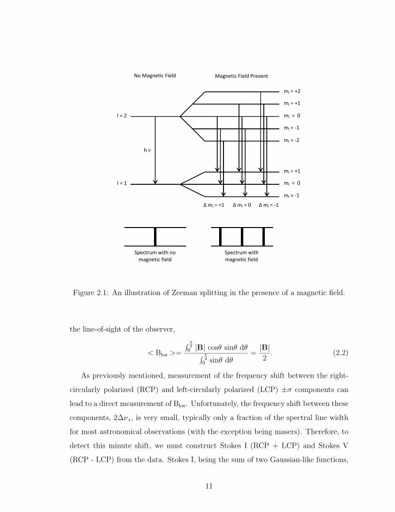
as the ±σ components. The production of these lines are governed by the selection

rules, allowing only transitions with ∆l = ±1 and ∆ml = ±1, 0, as illustrated in

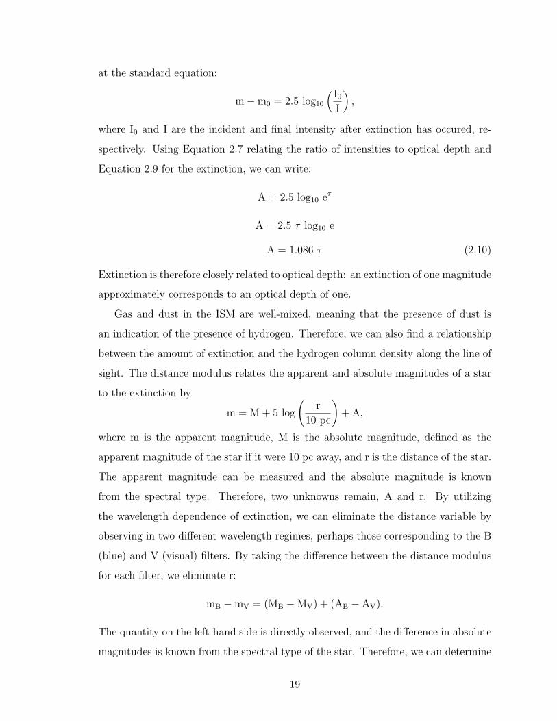
Figure 2.1.

When viewed along the magnetic field direction, the ±σ components appear op-

positely circularly polarized and are shifted relative to the π component by the fre-

quency given in Equation 2.1, while the unshifted π component is linearly polarized

along the field direction. When viewed perpendicular to the magnetic field, all three

components are linearly polarized, the ±σ components perpendicular to and the π

component parallel to the field direction. When viewed at intermediate angles, the

±σ components become elliptically polarized.

These polarization effects lead to the ability to observationally detect the Zeeman

effect. By observing the circular (or, more generally, elliptical) polarization effects

arising from the ±σ components, one can detect the frequency shift described in

Equation 2.1, and therefore determine the magnitude of the magnetic field along

the line-of-sight, Blos. It is important to emphasize that the Zeeman effect can only

reveal the line-of-sight component of the magnetic field rather than the total field

strength. Therefore, the measured Blos is a lower limit to the true strength of the

field. As a result, Zeeman results must be taken statistically with a large sample of

sources, assuming that the true field orientations vary throughout the sample. It is

possible to apply a statistical correction to the measured values of Blos to account for

the fact that only one component of the field is measured. For a large ensemble of

Zeeman measurements for which the field is randomly oriented with respect to the

10

ml = +1

ml = 0

ml = -1

ml = -2

ml = +2

ml = +1

ml = 0

ml = -1

l = 2

l = 1

No Magnetic Field Magnetic Field Present

h ν

Δ ml = 0 Δ ml = +1 Δ ml = -1

Spectrum with no magnetic field

Spectrum with magnetic field

Figure 2.1: An illustration of Zeeman splitting in the presence of a magnetic field.

the line-of-sight of the observer,

< Blos >=

∫ π2

0 |B| cosθ sinθ dθ∫ π2

0 sinθ dθ=|B|2

. (2.2)

As previously mentioned, measurement of the frequency shift between the right-

circularly polarized (RCP) and left-circularly polarized (LCP) ±σ components can

lead to a direct measurement of Blos. Unfortunately, the frequency shift between these

components, 2∆νz, is very small, typically only a fraction of the spectral line width

for most astronomical observations (with the exception being masers). Therefore, to

detect this minute shift, we must construct Stokes I (RCP + LCP) and Stokes V

(RCP - LCP) from the data. Stokes I, being the sum of two Gaussian-like functions,

11

will appear to the observer as a single Gaussian peaked at the unshifted frequency.

However, for Stokes V, the difference of two Gaussian-like functions each shifted with

respect to the other in frequency, will appear as the scaled-down derivative of the

Stokes I profile, where the scaling factor is proportional to the field strength. This

derivative ‘S’ curve is the classic signature of the Zeeman effect. However, due to

possible small gain differences in the two circular polarizations, a version of Stokes I

itself may also appear in Stokes V. Blos is then inferred by performing a linear least-

squares fit of the scaled versions of Stokes I to Stokes V via the equation

V(ν) = aI(ν) +

(zBcosθ

2

)dI(ν)

dν, (2.3)

where a is a scaling factor to account for necessary gain correction, z is the Zeeman

splitting factor and depends upon the atomic or molecular species observed (e.g.,

z = 2.8 Hz µG−1 for HI, 3.27 Hz µG−1 for 1665 MHz OH, and 1.96 Hz µG−1 for

1667 MHz OH), and θ is the angle between the field direction and the observer. By

convention, positive values of Blos correspond to the magnetic field oriented away

from the observer, while negative values indicate the field is towards the observer.

The least-squares fitting procedure also yields the uncertainty σ in the inferred Blos,

which is expected to be Gaussian-normal. Therefore, the probability distribution of

a single Zeeman measurement is Gaussian.

2.2 Atomic Hydrogen

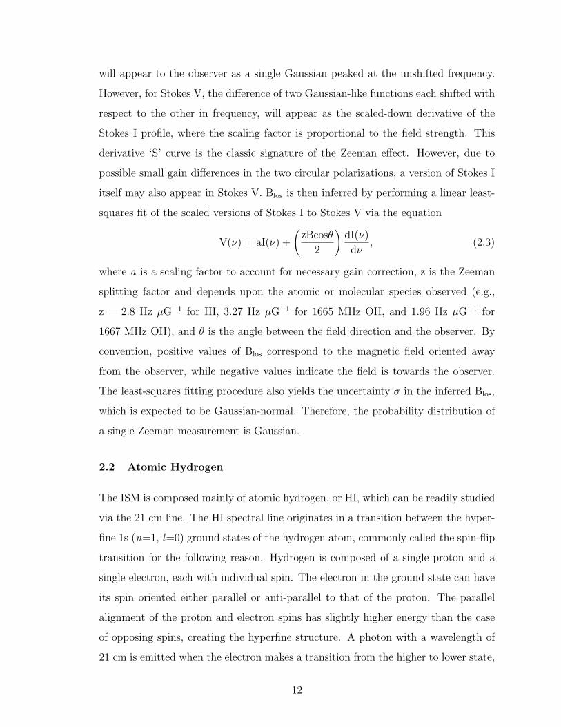
The ISM is composed mainly of atomic hydrogen, or HI, which can be readily studied

via the 21 cm line. The HI spectral line originates in a transition between the hyper-

fine 1s (n=1, l=0) ground states of the hydrogen atom, commonly called the spin-flip

transition for the following reason. Hydrogen is composed of a single proton and a

single electron, each with individual spin. The electron in the ground state can have

its spin oriented either parallel or anti-parallel to that of the proton. The parallel

alignment of the proton and electron spins has slightly higher energy than the case

of opposing spins, creating the hyperfine structure. A photon with a wavelength of

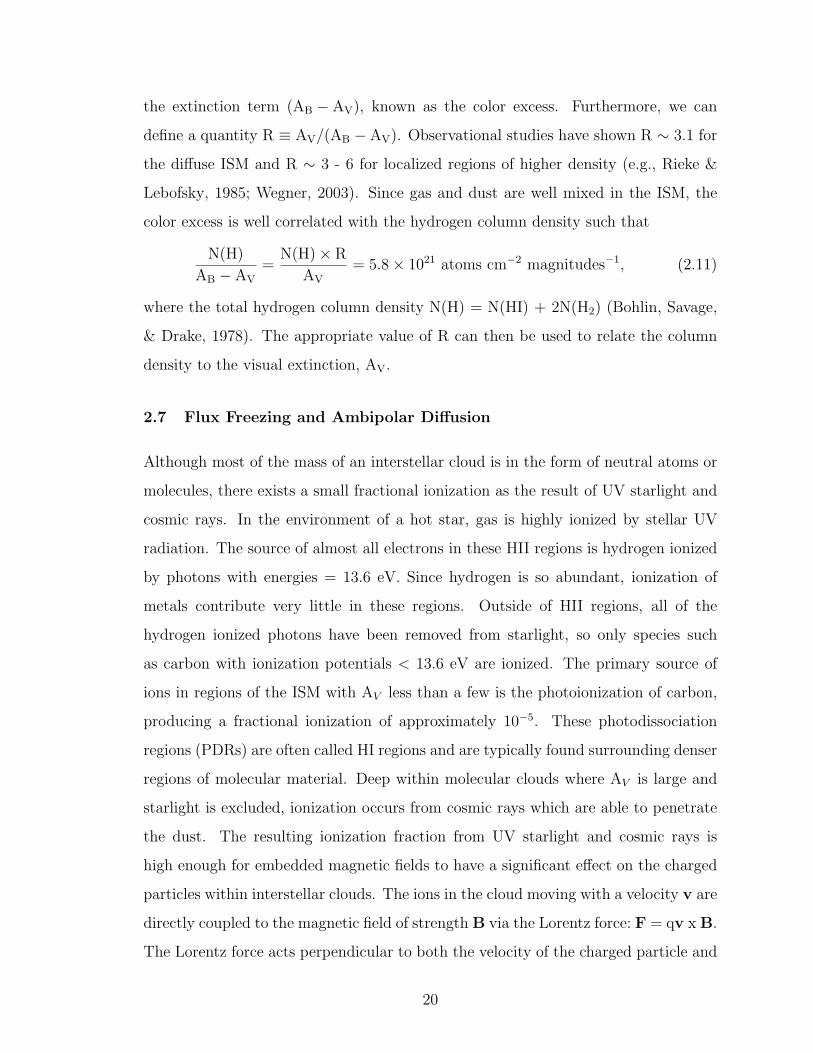
21 cm is emitted when the electron makes a transition from the higher to lower state,

12

flipping its spin (see Figure 2.2). This so-called spin-flip transition is a “forbidden”

transition, meaning that it violates the selection rules. Although dubbed forbidden,

the fact that HI can be observed suggests that it is not prohibited from occurring.

A forbidden transition is one that has a very low probability of occurring. The Ein-

stein A coefficient for HI, which represents the probability for spontaneous emission,

is extremely low; A10 ≈ 2.9 x 10−15 s−1, leading to a radiative half-life of about 11

million years. However, due to the sheer abundance of HI in the Universe, the 21 cm

transition can be easily studied.

Figure 2.2: The spin-flip transition in the hydrogen atom gives rise to the 21 cm radioline. This transition is the result of the release of a photon of wavelength 21 cm whenthe spins of the proton and electron flip from parallel to antiparallel.

The study of HI has been invaluable to the field of astronomy. For example, HI

observations have been used to determine the rotation curve of our Galaxy (e.g.,

Clemens, 1985). They have also been instrumental in measuring magnetic field

strengths throughout the Galaxy (e.g., Heiles & Troland, 2003a), which ultimately

inspired the research presented here.

2.3 The Hydroxyl Molecule

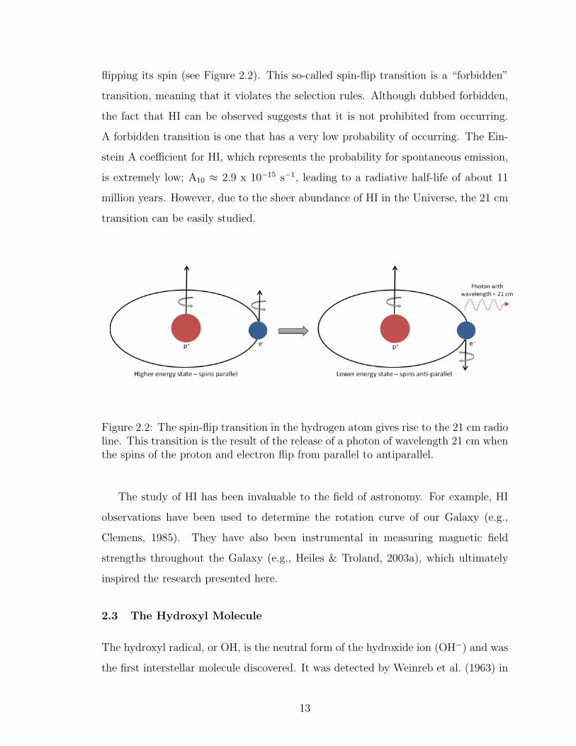
The hydroxyl radical, or OH, is the neutral form of the hydroxide ion (OH−) and was

the first interstellar molecule discovered. It was detected by Weinreb et al. (1963) in

13

the absorption spectrum of Cassiopeia A. As briefly discussed in Section 2.1, OH has

an unpaired electron and therefore is very sensitive to the Zeeman effect. The ground

state of OH has electronic angular momentum L=1 and spin angular momentum

S=1/2. Thus, by spin-orbit coupling, the total angular momentum is either J=3/2,

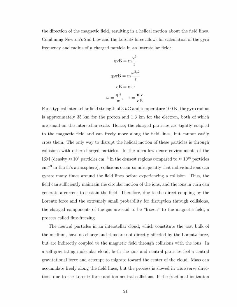
or J=1/2, leading to the 2Π3/2 and the 2Π1/2 rotational states. Due to the interaction

between the rotation of the nuclei and the unpaired electron in the outer shell, the

2Π3/2 state of OH undergoes Λ-doubling, splitting it into 2 states, with a separation

corresponding to approximately 1666 MHz (Robinson & McGee, 1967). This splitting

is shown in Figure 2.3, where these states are labeled with a ‘+’ and ‘-’ for the higher

and lower energy states, respectively. Due to hyperfine interactions with the nuclear

spin, each doublet state is further split into 2 levels, corresponding to F = J + I,

where I is the nuclear spin, equal to ±1/2. Transitions between these 4 independent

energy states result in the 18-cm ground state spectral lines at 1612, 1665, 1667, and

1720 MHz, as shown in Figure 2.3. In the presence of an external magnetic field, each

F state is split into 2F + 1 sublevels in the usual way, as described in Section 2.1,

above. This gives rise to the Zeeman effect in OH.

Figure 2.3: The 18 cm ground state transitions of the OH molecule.

The so-called OH main lines at 1665 and 1667 MHz obey the normal Zeeman

effect. That is, in the influence of an external magnetic field, their 2l+1 ml sublevels

are spaced such that the ±σ components are shifted by equal energy amounts to

14

either side of the π component in the triplet pattern. However, the splitting patterns

of the 1612 and 1720 MHz satellite lines of OH do not appear as a symmetric triplet

and therefore exhibit the anomalous Zeeman effect.

2.4 Excitation Temperature

Emission and absorption spectral lines are produced when atoms change energy levels

due to the emission or absorption of a photon. An atom may be excited to a higher

energy level in two ways: radiatively or collisionally. Radiative excitation occurs

when a photon of energy exactly equal to the difference between two energy levels

of the atom is absorbed. The result is an absorption spectrum with the spectral

line occurring at the frequency corresponding to the photon’s energy. Collisional

excitation occurs when a free particle, such as an electron, collides with an atom

and transfers some of its kinetic energy. This additional energy can excite the atom

to a higher state. No absorption spectrum is produced since this collisional process

does not involve any photons. Atoms prefer to be in the lowest possible energy state

rather than in an excited state. Therefore, a short time after excitation occurs, be it

a result of collision or photon absorption, the atom will return to its ground state by

emitting photons and producing an emission spectrum.

If the gas is in local thermal equilibrium (LTE) and collisional processes dominate

the excitation of atoms, then each excitation is balanced by a de-excitation. There-

fore, the population in a given state is unchanged in time. The relative populations

of two levels within an atom is governed by the Boltzmann equation:

nu

nl

=gu

gl

e−∆Eul

kTk , (2.4)

where nu and nl are the number densities of the upper and lower states, respectively,

gu and gl are the statistical weights, ∆Eul is the energy difference between the two

levels, k is the Boltzmann constant, and Tk is the kinetic temperature of the sys-

tem. However, in many scenarios radiative processes are also important and the level

populations cannot be determined through direct use of the Boltzmann equation. In

this case, the kinetic temperature is replaced by the excitation temperature Tex. The

15

excitation temperature is not a physical temperature, but rather a way to charac-

terize the level populations in non-LTE environments that do not strictly obey the

Boltzmann formula. In general, Tex 6= Tk, except for when the system is in LTE or at

very high densities when the excitation temperature approaches the kinetic temper-

ature. The value of Tex is positive except in systems in which the level populations

are inverted (nu > nl), such as masers. In the case of HI, the excitation temperature

is called spin temperature (Ts) to reflect that it represents the relative populations

between the parallel and anti-parallel proton and electron spin states responsible for

the 21-cm spin-flip transition.

When a bright background continuum source is present, a series of on- and off-

source observations can reveal excitation temperatures. On-source measurements,

with the telescope pointed at a background continuum source, will yield an absorption

profile. Off-source observations, with the radio telescope pointed so the continuum

source is out of the beam, determine the “blank sky” contribution Texp(ν). This is

called the expected profile and represents the line profile that one would observe at the

source’s position in the absence of the continuum source. Texp(ν) can be determined

with a single off-source pointing, for which the observer must assume that the gas

is uniform so the on- and off-source observations have the same physical properties.

Alternatively, several off-source measurements can be made in the vicinity of the

source and averaged to get a better representation of the gas in the direction of the

continuum source. The expected profile can either be in emission, absorption, or show

no structure, depending on whether Tex is greater than, less than, or approximately

equal to the brightness temperature of the background radiation field, respectively.

As discussed in Section 1.1, the ISM consists of multiple phases, two of which

are the CNM and the WNM. The CNM is solely responsible for observed absorption,

while both the CNM and WNM brightness temperatures contribute to the expected

profile:

Texp(ν) = TB,CNM(ν) + TB,WNM(ν). (2.5)

16

The CNM contribution to the expected profile is

TB,CNM(ν) = Tex(1− e−τ(ν)), (2.6)

where Tex is the excitation temperature and τ(ν) is the CNM opacity (see Section

2.5 for a discussion of opacity). Therefore, if the CNM contribution to the expected

profile and the optical depth can be determined from on- and off-source observations,

the excitation temperature can be calculated. A full discussion can be found in Heiles

& Troland (2003a).

2.5 Optical Depth and Column Density

Consider a bright continuum source that provides an intensity I0(ν). As the ray passes

through the ISM it is absorbed and scattered by the intervening interstellar material

such that only a fraction of the the initial intensity is observed at some distance x

from the continuum source. The observed intensity will depend on several factors

such as how far the ray has traveled, the density of the material, and the efficiency

with which the material absorbs or scatters light such that the initial intensity is

attenuated by an amount

dI = −I0κρdx,

where dI is the change in intensity, κ is the opacity or the absorption coefficient, ρ is

the density of the absorbing material, and dx is the distance traveled. To find the

final intensity, we integrate over the entire path length L:

∫ dI

I0=∫ L

0−κρdx

ln(

I

I0

)= −κρL

I = I0e−κρL

I = I0e−τ , (2.7)

where I is the final intensity and τ ≡ −κρL = optical depth. So, an optical depth of

0.5 means that the initial intensity is attenuated by a factor e−0.5.

17

The column density N describes the number of particles of a particular species

(e.g., H) in a cross sectional area of 1 cm2, integrated along a path:

N =∫

n ds.

In terms of the excitation temperature and optical depth, the column density can be

expressed as

N = C τν Tex ∆VFWHM, (2.8)

where ∆VFWHM is the full width at half maximum spectral line velocity width and C is

a constant equal to 4.11×1014, 2.28×1014, and 1.95×1018 for the 1665 and 1667 MHz

OH main lines and the 21-cm HI line, respectively (Crutcher, 1977; Heiles & Troland,

2003b; Roberts, 1995). Hydrogen column densities can be estimated through use

of a OH/H conversion ratio such that N(OH) = N(H) [N(OH)/N(H)]. This ratio

[N(OH)/N(H)] = 4 × 10−8 was determined by Crutcher (1979) through a study of

N(OH) toward stars of with known extinctions. The observed OH column density was

then compared to the hydrogen column density calculated from the known extinctions

(see Section 2.6).

2.6 Interstellar Extinction

The general concept of interstellar extinction was introduced in Section 1.1. Recall

that extinction is the number of magnitudes by which starlight is attenuated by the

combined effects of scattering and absorption by dust grains. The observed magnitude

m after extinction is described by the extinction A and incident magnitude m0 by

the relation

m = m0 + A. (2.9)

Very bright objects have negative magnitudes and dimmer objects have large values

of magnitude. The magnitude scale is logarithmic and set such that a difference of

5 magnitudes corresponds to a factor of 100 in intensity, or (I0/I) = 100(m−m0)/5.

Converting this to a base 10 scale and solving for the magnitude difference, we arrive

18

at the standard equation:

m−m0 = 2.5 log10

(I0I

),

where I0 and I are the incident and final intensity after extinction has occured, re-

spectively. Using Equation 2.7 relating the ratio of intensities to optical depth and

Equation 2.9 for the extinction, we can write:

A = 2.5 log10 eτ

A = 2.5 τ log10 e

A = 1.086 τ (2.10)

Extinction is therefore closely related to optical depth: an extinction of one magnitude

approximately corresponds to an optical depth of one.

Gas and dust in the ISM are well-mixed, meaning that the presence of dust is

an indication of the presence of hydrogen. Therefore, we can also find a relationship

between the amount of extinction and the hydrogen column density along the line of

sight. The distance modulus relates the apparent and absolute magnitudes of a star

to the extinction by

m = M + 5 log

(r

10 pc

)+ A,

where m is the apparent magnitude, M is the absolute magnitude, defined as the

apparent magnitude of the star if it were 10 pc away, and r is the distance of the star.

The apparent magnitude can be measured and the absolute magnitude is known

from the spectral type. Therefore, two unknowns remain, A and r. By utilizing

the wavelength dependence of extinction, we can eliminate the distance variable by

observing in two different wavelength regimes, perhaps those corresponding to the B

(blue) and V (visual) filters. By taking the difference between the distance modulus

for each filter, we eliminate r:

mB −mV = (MB −MV) + (AB − AV).

The quantity on the left-hand side is directly observed, and the difference in absolute

magnitudes is known from the spectral type of the star. Therefore, we can determine

19

the extinction term (AB − AV), known as the color excess. Furthermore, we can

define a quantity R ≡ AV/(AB − AV). Observational studies have shown R ∼ 3.1 for

the diffuse ISM and R ∼ 3 - 6 for localized regions of higher density (e.g., Rieke &

Lebofsky, 1985; Wegner, 2003). Since gas and dust are well mixed in the ISM, the

color excess is well correlated with the hydrogen column density such that

N(H)

AB − AV

=N(H)× R

AV

= 5.8× 1021 atoms cm−2 magnitudes−1, (2.11)

where the total hydrogen column density N(H) = N(HI) + 2N(H2) (Bohlin, Savage,

& Drake, 1978). The appropriate value of R can then be used to relate the column

density to the visual extinction, AV.

2.7 Flux Freezing and Ambipolar Diffusion

Although most of the mass of an interstellar cloud is in the form of neutral atoms or

molecules, there exists a small fractional ionization as the result of UV starlight and

cosmic rays. In the environment of a hot star, gas is highly ionized by stellar UV

radiation. The source of almost all electrons in these HII regions is hydrogen ionized

by photons with energies = 13.6 eV. Since hydrogen is so abundant, ionization of

metals contribute very little in these regions. Outside of HII regions, all of the

hydrogen ionized photons have been removed from starlight, so only species such

as carbon with ionization potentials < 13.6 eV are ionized. The primary source of

ions in regions of the ISM with AV less than a few is the photoionization of carbon,

producing a fractional ionization of approximately 10−5. These photodissociation

regions (PDRs) are often called HI regions and are typically found surrounding denser

regions of molecular material. Deep within molecular clouds where AV is large and

starlight is excluded, ionization occurs from cosmic rays which are able to penetrate

the dust. The resulting ionization fraction from UV starlight and cosmic rays is

high enough for embedded magnetic fields to have a significant effect on the charged

particles within interstellar clouds. The ions in the cloud moving with a velocity v are

directly coupled to the magnetic field of strength B via the Lorentz force: F = qv x B.

The Lorentz force acts perpendicular to both the velocity of the charged particle and

20

the direction of the magnetic field, resulting in a helical motion about the field lines.

Combining Newton’s 2nd Law and the Lorentz force allows for calculation of the gyro

frequency and radius of a charged particle in an interstellar field:

qvB = mv2

r

qωrB = mω2r2

r

qB = mω

ω =qB

m, r =

mv

qB.

For a typical interstellar field strength of 3 µG and temperature 100 K, the gyro radius

is approximately 35 km for the proton and 1.3 km for the electron, both of which

are small on the interstellar scale. Hence, the charged particles are tightly coupled

to the magnetic field and can freely move along the field lines, but cannot easily

cross them. The only way to disrupt the helical motion of these particles is through

collisions with other charged particles. In the ultra-low dense environments of the

ISM (density ≈ 106 particles cm−3 in the densest regions compared to ≈ 1019 particles

cm−3 in Earth’s atmosphere), collisions occur so infrequently that individual ions can

gyrate many times around the field lines before experiencing a collision. Thus, the

field can sufficiently maintain the circular motion of the ions, and the ions in turn can

generate a current to sustain the field. Therefore, due to the direct coupling by the

Lorentz force and the extremely small probability for disruption through collisions,

the charged components of the gas are said to be “frozen” to the magnetic field, a

process called flux-freezing.

The neutral particles in an interstellar cloud, which constitute the vast bulk of

the medium, have no charge and thus are not directly affected by the Lorentz force,

but are indirectly coupled to the magnetic field through collisions with the ions. In

a self-gravitating molecular cloud, both the ions and neutral particles feel a central

gravitational force and attempt to migrate toward the center of the cloud. Mass can

accumulate freely along the field lines, but the process is slowed in transverse direc-

tions due to the Lorentz force and ion-neutral collisions. If the fractional ionization

21

is low, as is the case for molecular clouds, the frequency of ion-neutral collisions de-

creases and the field becomes decoupled from the neutral material. A relative drift

between charged and neutral particles develops as the neutral particles are able to

diffuse through the ions and drift in response to the gravitational potential. This is a

process called ambipolar diffusion (APD) and, when flux freezing is in place, allows

mass to accumulate without significant change in magnetic flux. The effect of APD

is to allow an initially magnetically supported molecular cloud to evolve and collapse

under gravitational pressure due to the increased mass.

The evolution of a molecular cloud is controlled by the process with the largest

time scale. The ambipolar diffusion timescale is given by Hartquist & Williams (1989)

to be

tAPD = 4× 1013 χi years,

where χi = ni

nHis the fractional ionization, or the ratio of the number density of

charged to neutral particles. Here, nH = (n(H)+2n(H2)) is the total hydrogen num-

ber density in cm−3. Another relevant time scale for molecular clouds is that of

gravitational free fall collapse, given by Spitzer (1978) as

tff =

(3π

32Gρ

)1/2

seconds =4.3× 107

(nH)1/2years.

In dense molecular cores, where the fractional ionization is low (χi ≈ 10−7) and hy-

drogen densities are high (nH ≈ 106), tAPD ≈ 4 × 106 years and tff ≈ 4 × 104 years.

Therefore, the time scale for ambipolar diffusion can be significantly greater than the

free fall time, indicating that APD is the dominating process in the evolution of dense

molecular clouds that are supported by flux freezing. However, in the envelopes of

molecular clouds, where the hydrogen densities are lower and gas is less shielded from

ionizing starlight, the fractional ionization may be greater than 10−5 (Mouschovias

& Morton, 1991). This increase in ionization provides better “freezing” of the neu-

tral matter to the magnetic field lines and less relative drift between the ions and

neutral material. Therefore, APD is less effective in the highly ionized, lower density

envelopes of interstellar clouds than in molecular cores.

22

2.8 Mass-to-Flux Ratio

As discussed in the previous section, if embedded magnetic fields are coupled to

the interstellar gas through flux freezing, they can have a profound impact on the

evolution of molecular clouds and their eventual collapse to form stars. The fate

of an interstellar cloud depends on the ratio of the forces of confinement and those

of support. The dominate force that acts to confine a cloud is gravity, while it is

expected that turbulence and magnetic pressure contribute approximately equally

in providing internal support against gravitational collapse if the cloud is in near

equilibrium (McKee et al., 1993). The significance of the support provided by the

magnetic field alone can be determined by the mass-to-flux ratio, a comparison of

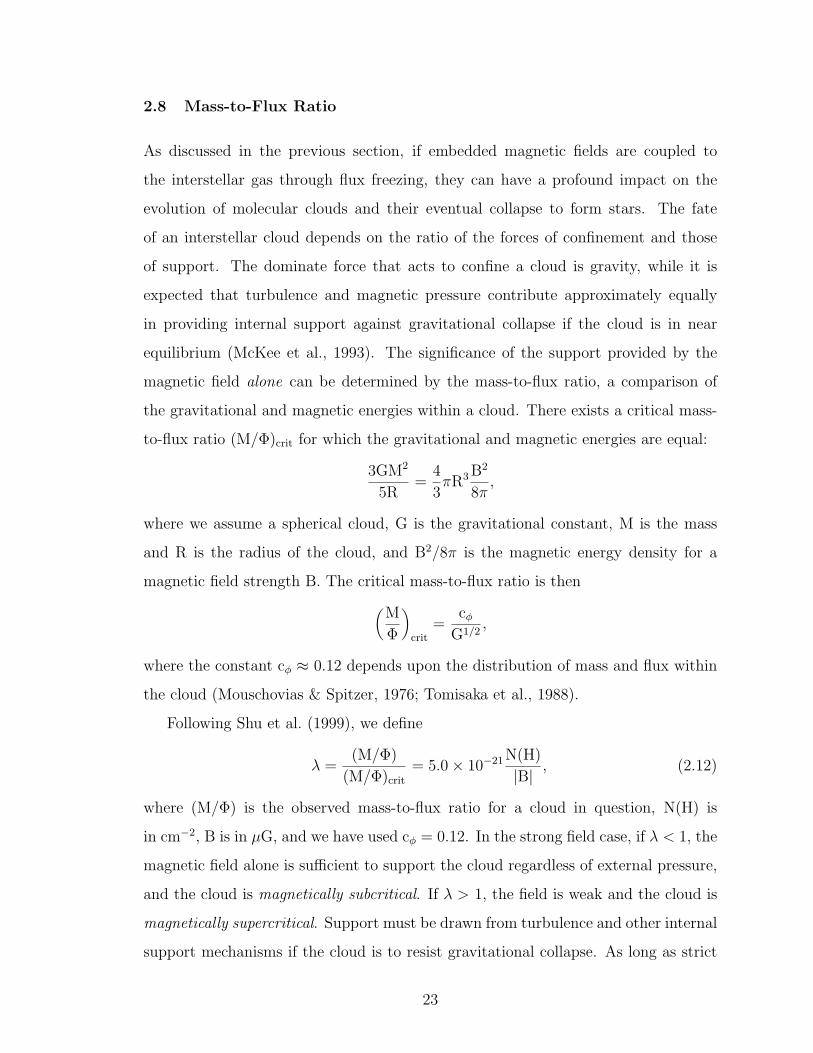
the gravitational and magnetic energies within a cloud. There exists a critical mass-

to-flux ratio (M/Φ)crit for which the gravitational and magnetic energies are equal:

3GM2

5R=

4

3πR3 B2

8π,

where we assume a spherical cloud, G is the gravitational constant, M is the mass

and R is the radius of the cloud, and B2/8π is the magnetic energy density for a

magnetic field strength B. The critical mass-to-flux ratio is then(M

Φ

)crit

=cφ

G1/2,

where the constant cφ ≈ 0.12 depends upon the distribution of mass and flux within

the cloud (Mouschovias & Spitzer, 1976; Tomisaka et al., 1988).

Following Shu et al. (1999), we define

λ =(M/Φ)

(M/Φ)crit

= 5.0× 10−21 N(H)

|B|, (2.12)

where (M/Φ) is the observed mass-to-flux ratio for a cloud in question, N(H) is

in cm−2, B is in µG, and we have used cφ = 0.12. In the strong field case, if λ < 1, the

magnetic field alone is sufficient to support the cloud regardless of external pressure,

and the cloud is magnetically subcritical. If λ > 1, the field is weak and the cloud is

magnetically supercritical. Support must be drawn from turbulence and other internal

support mechanisms if the cloud is to resist gravitational collapse. As long as strict

23

flux freezing is in place, the value of λ will remain constant throughout core evolution.

However, if the fractional ionization within a cloud is sufficiently low for ambipolar

diffusion to be important, a magnetically supported subcritical cloud may evolve into

a supercritical state over time and collapse as neutral matter drifts relative to ions,

increasing the central mass but not the flux.

It is important to emphasize that the mass-to-flux ratio only determines the sup-

port provided to a molecular cloud by the magnetic field, without regard to other

support mechanisms such as turbulence. If clouds are in near equilibrium between

support and confinement, (McKee et al., 1993) argue that the magnetic field is ex-

pected to only supply approximately half of the required support, with turbulence

providing the other half. Therefore, a cloud that is critical overall would be ex-

pected to be magnetically supercritical by a factor of 2, since the support is divided

approximately equally between magnetic fields and turbulence.

The mass-to-flux ratio lends itself to observational measurement since M/Φ ∝N/B,

where N is the column density and B is the magnetic field strength, which, in this

dissertation, is determined via the Zeeman effect. It is important to note that since

the Zeeman effect only reveals the line-of-sight magnetic field Blos, our determina-

tions of B are always lower limits to the total field strength with Φ underestimated

by cosθ. In addition, the column density should be measured parallel to the magnetic

field and along the minor axis of the cloud. However, we only sample the line-of-

sight column density without regard to cloud orientation, such that the path length

is too long by 1/cosθ and the mass is overestimated (Crutcher, 1999). Due to these

caveats, any survey of the mass-to-flux ratio in molecular clouds must be done in a

statistical manner with many independent measurements of λ to infer astronomically

meaningful information. The statistical correction for a large sample with random

cloud orientations is

M/Φ =∫ π/2

0

Mobscosθ

Φobs/cosθsinθdθ =

1

3

(M

Φ

)obs

. (2.13)

Copyright c© Kristen Lynn Thompson, 2012.

24

Chapter 3

Instrumentation and Methodology

3.1 Arecibo Telescope

The Arecibo telescope1, located in Arecibo, Puerto Rico, is the world’s largest and

most sensitive single-dish radio telescope. The primary reflecting dish has a diameter

of 305 meters and is situated in a natural karst sinkhole. Suspended 450 feet above

the dish is the platform, which houses the telescope’s receiver system.

When attempting to determine magnetic field strengths using the Zeeman effect, it

is necessary to be able to discern spectral lines from background noise. The ability of

a telescope to distinguish a signal from random background noise is called sensitivity.

The sensitivity of a telescope depends upon its ability to collect light. Therefore,

the Arecibo telescope, with the largest collecting area in the world, has the ability

to achieve greatest sensitivity among all telescopes. Whereas other telescopes may

require several hours observing a radio source to achieve the desired sensitivity, with

Arecibo it may take just a few minutes. This characteristic makes the use of this

instrument essential for our project to determine mass-to-flux ratios in molecular

clouds, which is presented in this dissertation. When using the Arecibo telescope, we

make use of several different observing methods to make the most efficient use of the

telescope and achieve our science goals. These methods are discussed below.

3.1.1 Position Switching

A telescope collects all radiation that lies within a thin column through the sky along

the line-of-sight, not just the signal emanating from the desired target source. In

addition, telescope receiver systems may introduce various instrumental effects into

1The Arecibo Observatory is part of the National Astronomy and Ionosphere Center (NAIC),

a national research center operated by SRI International, USRA, and UMET, under a cooperative

agreement with the National Science Foundation (NSF).

25

astronomical observations. It is therefore necessary to implement various methods

that are designed to mitigate the systematic and instrumental effects and isolate the

signal from the desired research target.

The most straight forward method of eliminating unwanted “background” noise is

to apply the position switching technique. Using this technique, the observer moves

the telescope between a signal (on-source) and reference (off-source) position at regu-

lar intervals during the observation period. Optimally, the off-source position would

be chosen to be a location void of radio sources that is spatially near and at roughly

the same elevation as the on-source position, ensuring that the same environment is

being sampled at both positions. The on-source observation measures the signal from

the target source plus the background, while the off-source measurement character-

izes the background only. Signals from the two positions are then subtracted to yield

the signal from the desired source.

This method is not very efficient, owing to the necessity to spend as much as

50% of observing time off-source. A decrease in on-source observation time leads to a

decrease in sensitivity, something not desirable for Zeeman observations. Therefore,

we do not make extensive use of this method.

3.1.2 In-Band Frequency Switching

A second method commonly used for data calibration is in-band frequency switching.

In this mode, the reference (off-source) spectrum is created by shifting the center

frequency of the local oscillator. If the frequency shift is small enough, both the

signal and reference spectra will show the spectral line. The calibration then occurs

by computing (signal - reference) / reference. The result will be a single spectrum

with the spectral line appearing twice, once in emission and once in absorption. The

spectrum can then be “folded” to produce a√

2 decrease in noise. This technique

is more desirable than position switching since there is less overhead as 100% of

observation time can be spent observing the target source. In addition, calibration

does not require an emission-free off-source reference position when observing a region

with complicated emission structure. However, the primary drawback is that the

26

spectral baselines may not be as flat as with position switching. This is due to each

frequency-switched observation having its own spectral bandpass shape, which may

not be entirely cancelled in the resultant spectrum. If the lines are narrow, and the

frequency shift is small, this method works quite well.

This method is the most desirable for our Arecibo telescope Zeeman observations

since sensitivity is of primary importance to the success of the project. Therefore,

the majority of our observations implement this technique.

3.1.3 Z16 Observing Pattern

Both methods described above have important drawbacks in addition to the over-

head time incrued by position switching and the residuals in the spectral baselines

introduced by frequency switching. The position switching method does not take into

account spatial variations in the radiation field around the target source and limi-

tations to analysis capabilities are introduced when true off-source observations are

not available, as for in-band frequency switching. One way to account for these is to

use the so-called Z16 observing pattern, described in Heiles & Troland (2003a). The

Z16 pattern consists of one on-source and 16 off-source pointings, with the off-source

positions arranged as two concentric circles of 8 pointings each with radii of 1 and√

2 half-power beam widths (see Figure 3.1). For 21-cm HI observations at Arecibo,

these offsets are equal to 3.4’ and 4.8’. The locations of these off-source observations

allow for the determination of both the first and second derivatives of background sky

emission, producing more accurate predictions of spatial variations in the vicinity of

the target source than the traditional position switching method. This is especially

important for HI observations, for which emission is variable and emanates from all

directions. Off-source observations dominate available time, as only approximately

40% of observing is spent on-source. This method was used for all HI observations

discussed in this dissertation, as well as for a small portion of the Galactic molecular

cloud OH observations.

27

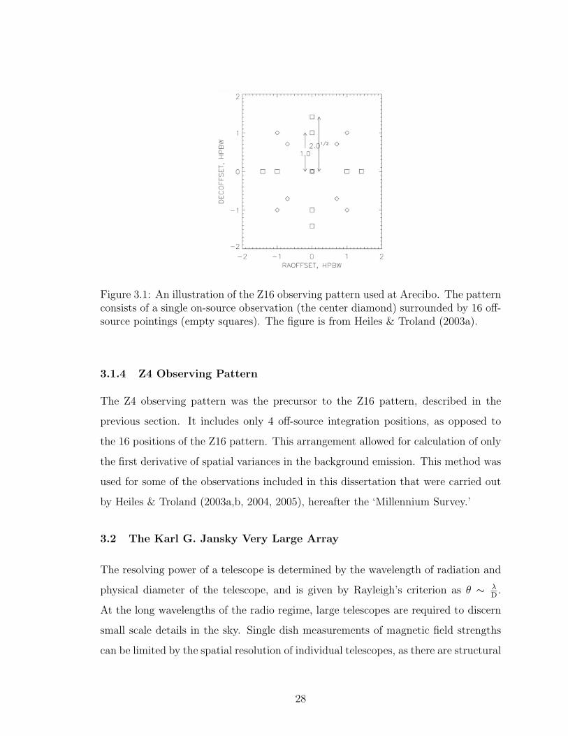
Figure 3.1: An illustration of the Z16 observing pattern used at Arecibo. The patternconsists of a single on-source observation (the center diamond) surrounded by 16 off-source pointings (empty squares). The figure is from Heiles & Troland (2003a).

3.1.4 Z4 Observing Pattern

The Z4 observing pattern was the precursor to the Z16 pattern, described in the

previous section. It includes only 4 off-source integration positions, as opposed to

the 16 positions of the Z16 pattern. This arrangement allowed for calculation of only

the first derivative of spatial variances in the background emission. This method was

used for some of the observations included in this dissertation that were carried out

by Heiles & Troland (2003a,b, 2004, 2005), hereafter the ‘Millennium Survey.’

3.2 The Karl G. Jansky Very Large Array

The resolving power of a telescope is determined by the wavelength of radiation and

physical diameter of the telescope, and is given by Rayleigh’s criterion as θ ∼ λD.

At the long wavelengths of the radio regime, large telescopes are required to discern

small scale details in the sky. Single dish measurements of magnetic field strengths

can be limited by the spatial resolution of individual telescopes, as there are structural

28

limitations to how large a single instrument can physically be made. In the case of

a radio interferometer, several telescopes work together such that resolving power is

determined by the maximum spacing between telescopes, rather than the diameter

of a single telescope.

One such radio interferometer is the Karl G. Jansky Very Large Array. The Jansky

VLA is operated by the National Radio Astronomy Observatory2 (NRAO) and is a

radio interferometer situated on the plains of San Agustin near Socorro, New Mexico.

Once known as simply the Very Large Array, the instrument was renamed in March

2012 in the midst of a major hardware upgrade to honor the contributions of the

founder of radio astronomy. The Jansky VLA consists of 27 independent antennas,

each with a diameter of 25 meters, arranged along the 3 arms of a ‘Y’ shape. They all

work together to build one of the most powerful tools in radio astronomy today. Each

antenna in the Jansky VLA can be moved to provide maximum antenna separations

ranging from 1.0 to 36.4 km, depending on which configuration the observer uses.

An interferometer, such as the Jansky VLA, works by simultaneously collecting

data with several antennas. There are N(N-1) possible antenna pairs within the array,

where N is the number of individual antennas. A single observation of a source for

a pair of antennas produces two points (since the antennas are reversible) in the

2-dimensional so-called u-v Fourier plane. The location of the data points in the

u-v plane indicate the east-west (u) and north-south (v) components of the baseline

between the antennas, as seen by the source. For each such point in the u-v plane,

the detected signal yields a value of the complex visibility function that is one spatial

Fourier component of the sky brightness distribution. The complex visibility consists

of two parts: the visibility amplitude, which is a measure of the detected flux from

the source, and the visibility phase, which provides information about the source

position.

Each pair of antennas can only provide resolution of the source in the direction

parallel to a line connecting the telescopes. However, as the Earth rotates the pro-

2The National Radio Astronomy Observatory is a facility of the National Science Foundation

operated under a cooperative agreement by Associated Universities, Inc.

29

jected baseline between each pair of antennas changes. As seen from the source,

each baseline traces out an ellipse with one telescope at the center. Therefore, by

tracking a target for an extended amount of time, one can determine the complete

2-dimensional structure of the radio source in the sky. Large arrays of telescopes

making repeated observations as the Earth rotates provide additional points in the

Fourier plane, and therefore additional complex visibility Fourier components. With

sufficient coverage of the u-v plane, the Fourier transform of the complex visibility

function produces a reasonable approximation of the true brightness distribution.

This is another advantage of interferometric observations over the single dish mea-

surements: interferometers can provide 3-D spectral line images over some spatial

region, whereas single dish observations only provide one spectrum per pointing.

The project in this dissertation aimed at determining magnetic field strengths in

the center of the Milky Way has made use of the Jansky VLA.

Copyright c© Kristen Lynn Thompson, 2012.

30

Chapter 4

Determination of the Mass-to-Flux Ratio in Molecular Clouds

4.1 Introduction

The details of the star formation process are not yet well understood, despite many

theoretical and observational studies. It has long been known that stars form in the

gravitational collapse of an interstellar molecular cloud. However, the evolution of

self-gravitating molecular clouds depends on the ratio of internal energies of support

to external energies of confinement. In the absence of internal support mechanisms,

a molecular cloud would undergo gravitational collapse and form stars on the free-

fall time scale, described in Section 2.7. This would lead to a star formation rate of

approximately 250 M� yr−1, which is far greater than the observed formation rate

of ∼ 3 M� yr−1 (McKee, 1999). Therefore, molecular clouds appear to be forming

stars inefficiently, suggesting that there must be some means of internal support

that is hindering the gravitational collapse of molecular clouds and lengthening cloud

lifetimes beyond the free-fall time. Any successful theory of star formation must

account for this inefficiency. Two prevailing theories of star formation have emerged,

one placing emphasis on the support provided by magnetic fields, and the other on

turbulence.

The magnetically driven model of star formation suggests that ambipolar diffu-

sion (discussed in Section 2.7) plays a crucial role in the evolution of molecular clouds

(Shu et al., 1999; McKee, 1999). This theory suggests that clouds that are initially

magnetically supercritical (see Section 2.8) will collapse under gravitational pressure

on relatively short timescales, forming high-mass stars. If the magnetic field does not

provide enough support to prevent the onset of gravitational collapse, it will not be

able to halt the process once it has begun. Molecular clouds that are magnetically

subcritical at formation, and are therefore supported by the magnetic field, will over

time become unstable and collapse to form low-mass stars through the ambipolar

31

diffusion process. Both charged and neutral particles in the cloud are coupled to

embedded magnetic fields, the ions directly by the Lorentz force and the neutrals

indirectly by collisions. The neutrals are able to slowly drift relative to the ions and

gravitationally contract, increasing the local mass while leaving the flux unchanged.

When the mass of the core exceeds the critical mass, the core becomes supercritical

and undergos gravitational collapse, forming stars in the process. Since the envelopes

of clouds are less shielded from ionizing radiation, flux freezing is more efficient in

these regions, and thus the timescale for ambipolar diffusion is longer than in the

cores. Therefore, the higher density cores may become supercritical and collapse,

but the magnetic flux remains in the still subcritical envelope of the star, providing

a means for angular momentum to be transferred from the system. The time scale

for ambipolar diffusion is significantly longer than the time for free-fall collapse, al-

lowing for cloud lifetimes longer than the free-fall timescale and accounting for the

inefficiency of star formation.

The turbulence driven model suggests that star formation is driven by supersonic

turbulence within the clouds (Mac Low & Klessen, 2004). In this theory, clouds

form intermittently at the intersections of supersonic flows in the ISM. Usually, these

clouds dissipate, but occasionally they can become gravitationally bound and collapse

to form stars. This theory accounts for the inefficiency of star formation in that only

a small fraction of the clumps become self-gravitating and undergo collapse. Unlike

the magnetically driven model, this theory is able to account for the formation of both

high- and low-mass stars using the same formulation. Magnetic fields are present in

this theory, but they are very weak and do not affect the process. The cloud cores

are therefore expected to be critical to slightly supercritical.

To distinguish between these two theoretical models of star formation, it is im-

portant to observationally determine magnetic field strengths in molecular clouds to

see if they are weak and support the supercritical argument of the turbulence driven

model, or if they are strong, favoring the magnetically driven ambipolar diffusion

model. The relevant parameter is the mass-to-flux ratio λ described in Section 2.8.

The critical value of this ratio, λ = 1, represents the case where the gravitational and

32

magnetic energies of a cloud are equal. If λ > 1, the cloud is magnetically supercrit-

ical and the gravitational energy dominates, leading to cloud collapse. If λ < 1, the

cloud is magnetically subcritical and the magnetic field supports the cloud against

gravitational collapse. The ambipolar diffusion model predicts that λ should be < 1

in the intercore regions of molecular clouds and ≈ 1 in the cores. If core collapse has

already begun, one would find λ > 1. However, the collapse proceeds quickly once it

has begun, so it is expected that values greater than 1 are rare. If magnetic fields are

truly too weak to be physically important, as the turbulence model implies, the value

of λ may take any value greater than 1, but very weak fields imply λ >> 1. The

determination of the mass-to-flux ratio can therefore be an effective tool to establish

the driving theory behind star formation.

The Zeeman effect provides the only technique for measuring magnetic field strengths

in molecular clouds (see Section 2.1). However, due to the difficulty involved in mea-

suring the small frequency shifts in the right- and left-circularly polarized components

of radio frequency spectral lines, Zeeman measurements are scarce. In addition, Zee-

man studies must be done in a statistical manner owing to the random orientations of

molecular clouds in the plane of the sky. It is clear that more observations are needed

to definitively associate the star formation process with either the magnetically driven

or turbulence driven theory.

4.2 Previous Studies

There have been several previous studies aimed at determining the mass-to-flux ratio

in molecular clouds. Molecular cloud magnetic field strengths have been determined

through observations of HI, OH, and CN. These three species measure the field over

a wide range of densities in the ISM from diffuse atomic gas to dense molecular cores:

HI samples densities ranging ∼ 1 - 100 cm−3, OH densities from ∼ 102 − 104 cm−3,

and CN reveals densities of ∼ 105 − 106 cm−3.

Owing to the difficulty of detecting the Zeeman effect in radio frequency spec-

tral line observations, only 27 sensitive measurements of magnetic field strengths in

molecular clouds were made prior to 1999. Crutcher (1999) summarized the results

33

of these studies and their implications for star formation theory. The Zeeman obser-

vations included results from measurements using HI, OH, and CN and were aimed

at dense cloud cores or HII regions near newly formed stars. Calculations of the

mass-to-flux ratio from these studies reveal clouds that are supercritical (gravitation-

ally dominated) by a factor of approximately 2. In addition, it was concluded that

gas velocities in the clouds are supersonic by about a factor of 5 and the gas may

provide significant support. However, it was also found that the ratio of thermal to

magnetic pressures βp ≈ 0.04, suggesting that magnetic effects are dominate over

thermal effects. Therefore, although magnetic fields alone cannot fully support the

cloud against gravitational support, they may still play a significant role.

The next significant survey of the mass-to-flux ratio in molecular clouds was by

Bourke et al. (2001), adding to existing measurements in the northern hemisphere

and extending the study into the southern hemisphere. Observations of OH ab-

sorption lines toward molecular clouds were obtained using both the NRAO 43 m

Green Bank telescope and the Australia Telescope National Facility (ATNF)1 Parkes

64 m telescope. Observations of 23 molecular clouds yielded a Zeeman detection of

Blos = 38 ± 3 µG towards RCW 38, a possible detection of Blos = -203 ± 24 µG

toward RCW 57, and provided upper limits to the magnetic field strength for 21

additional components. Calculations of the mass-to-flux ratio are in agreement with

Crutcher (1999): molecular clouds appeared to be supercritical by a factor of 2 - 3,

and no clear examples of a magnetically subcritical clouds were found.

An extensive survey of Zeeman splitting measurements using the 21-cm HI line in

absorption was undertaken by Heiles & Troland (2005, and references therein). This

“Millennium Survey” revealed magnetic field strengths and column densities along

the line-of-sight toward 79 continuum sources. Target sources were not selected to

specifically lie behind molecular clouds, resulting in a sample that preferentially fa-

vors the determination of field strengths and column densities in diffuse regions of

the interstellar medium. Therefore, it is important to note that this study is much

1The Australia Telescope is funded by the Commonwealth of Australia for operation as a Na-

tional Facility managed by CSIRO.

34

different from the others in this section since it samples interstellar gas that is diffuse,

not molecular, in nature. Mass-to-flux ratios derived from these measurements sug-

gest that the diffuse ISM material probed by HI lies in the subcritical regime. That

is, sufficient support is provided by magnetic energy to prevent gravitational collapse

of the material.

Troland & Crutcher (2008) performed an OH emission line survey of magnetic

field strengths toward 34 dark cloud cores, the sites of low-mass star formation.

Nine new probable Zeeman detections were found at the 2.5σ level. In agreement

with previous studies, calculations reveal λ ≈ 2, such that dark clouds are therefore

slightly supercritical. Also, the ratio of turbulent to magnetic energies βturb was found

to be ≈ 2.4, indicating that turbulent energy exceeds magnetic energy. The authors

point out that these results do not distinguish between the two competing theories

of star formation, but rather support both. If λ had been significantly higher than 2,

then the magnetically driven model could have been ruled out since the clouds would

be clearly supercritical. On the other hand, had λ been significantly lower than 2,

then magnetic fields would play a crucial role in the support of molecular clouds and

the turbulence driven model could have been eliminated. Therefore, a clear conclusion

as to the role of magnetic fields in star formation could not be determined.

Falgarone et al. (2008) conducted a CN emission survey of Zeeman observations

toward 14 dense cloud cores using the IRAM-30 m telescope. They report 8 prob-

able detections of the Zeeman effect and find that the clouds are critical to slightly

supercritical with λ ≈ 1 to 4, although they point out the uncertainties in column

density and only observing Blos may affect the results. In addition, they find that the

magnetic and turbulent energies are approximately equal.

Figure 4.1 shows the Blos plotted against the total hydrogen column density N(H)

for the collection of all previous results. The diagonal line represents the “criti-

cal line,” where the magnetic and gravitational energies are equal. Therefore, any

data point that lies above the line is magnetically subcritical, while those below

the line are magnetically supercritical. Error bars represent 1σ uncertainties in the

strength of the line-of-sight field. The results shown span three species of observa-

35

tions: lowest column densities (N(H) < ∼ 1.5 × 1021) are sampled by HI, mid-range

densities (1.5 × 1021 < N(H) < 5 × 1022) by OH, and the highest density regions

(N(H) < 5 × 1022) by CN. It is clear that diffuse non-self-gravitating interstellar

clouds sampled by atomic hydrogen are subcritical, while there are no clear subcrit-

ical detections of molecular gas in either OH or CN. However, it is important to

realize that the derived N(H) is uncertain to a factor of ∼ 2, so the results of these

previous studies are consistent with molecular clouds being approximately magneti-

cally critical with magnetic and gravitational energies nearly balanced. More studies

are needed to decisively determine the extent of the role of magnetic fields in star

formation.

4.3 Project Goals

The existing observations discussed in the previous section have only sampled the

diffuse regions of the ISM and those regions associated with molecular cores. One

question that is left to be answered is what role do magnetic fields play in the general

intercore regions of molecular clouds? If a complete understanding of the evolution of

molecular clouds as a whole is to be found, the mass-to-flux ratio in the envelopes of

molecular clouds must also be examined. We have therefore conducted the first ob-

servational survey directed at determining the role of magnetic fields in the evolution

of molecular clouds as a whole.

We aim to measure the mass-to-flux ratio in the intercore regions of molecular

clouds by searching for the Zeeman effect in OH and HI absorption lines. We also

determine OH excitation temperatures in GMCs by utilizing a series of on- and off-

source observations, as described in Section 2.5. Observations consist of lines-of-

sight such that we sample molecular clouds distributed at different Galactocentric

distances and that are known to be responsible for forming both high- and low-mass

stars. Such a diverse sample may allow for classification of magnetic field strengths

as a function distance and may reveal a link between magnetic field strength and

the characteristics of stars that may eventually form from the envelope gas. Also,

a sample that is comprised of sources distributed throughout the sky may allow for

36

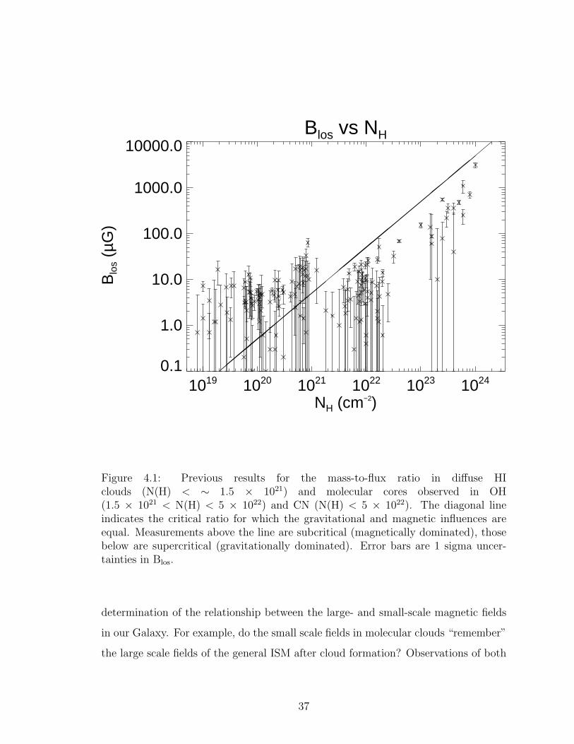
Blos vs NH

1019 1020 1021 1022 1023 1024

NH (cm−2)

0.1

1.0

10.0

100.0

1000.0

10000.0

Blo

s (µ

G)

Figure 4.1: Previous results for the mass-to-flux ratio in diffuse HIclouds (N(H) < ∼ 1.5 × 1021) and molecular cores observed in OH(1.5 × 1021 < N(H) < 5 × 1022) and CN (N(H) < 5 × 1022). The diagonal lineindicates the critical ratio for which the gravitational and magnetic influences areequal. Measurements above the line are subcritical (magnetically dominated), thosebelow are supercritical (gravitationally dominated). Error bars are 1 sigma uncer-tainties in Blos.

determination of the relationship between the large- and small-scale magnetic fields

in our Galaxy. For example, do the small scale fields in molecular clouds “remember”

the large scale fields of the general ISM after cloud formation? Observations of both

37

OH and HI will provide new information about the relative abundance of atomic and

molecular gas in GMCs. This relative abundance is currently not well-determined.

As a result of this survey, we aim to expand upon the existing knowledge of

magnetic fields in molecular clouds, specifically, in the intercore regions. In addi-

tion to calculating the mass-to-flux ratios in these regions, we hope to contribute to

the understanding of parameters such as OH excitation temperature and atomic to

molecular gas ratios.

4.4 Selection of Targets

Potential targets were selected from extra-galactic continuum sources that lie behind

galactic molecular clouds visible from Arecibo. Molecular clouds within the declina-

tion range of Arecibo were identified from the CO maps of Dame (2001), and bright

(Sν > 0.5 Jy) continuum sources spatially coincident with suitable molecular clouds

were selected using the NRAO VLA Sky Survey (NVSS) (Condon et al., 1998). A

figure of merit for each potential target source was determined via WCO × Sν , where

WCO =∫

Tdv is the velocity integrated CO emission from the data cubes of Dame

(2001) and is an indicator of the column density of molecular gas. Extra-galactic

sources possessing the largest figure of merit were selected, provided they were not

previously observed as part of the Millennium Survey (Heiles & Troland, 2003a,b,

2004, 2005). Prior to Zeeman observations, our target list was further narrowed by

a series of short position switching measurements (see Section 3.1) to determine OH

absorption line strengths in the direction of each source. We selected target sources

with strong and narrow absorption lines for our final target list (since sensitivity to

Blos ∝ line strength and also ∝ ∆v−1). This reduction was necessary due to lim-

ited telescope time (400 hours) and the high level of sensitivity required to detect

the Zeeman effect in radio frequency spectral lines. The amount of time needed to

acquire the desired sensitivity of σ(Blos) ≈ 5 µG was estimated using the sensitivity

calculator of Troland (1990). For a 1 Jy source with an assumed peak optical depth

of τ0 = 0.1 and FWHM velocity width ∆v = 1 km s−1, we predict that ≈ 23 hours

of on-source integration time on the 1667 MHz line is required. Of course, the total

38

observing time is greater if not all time is spent integrating on the source (with the

Z16 observing method, for example). After data has been separately calibrated and

reduced, one can combine the results from the two OH main lines, leading to a further√

2 reduction of σ(Blos).

Our final observation list consisted of 16 target sources. These sources are diverse,

in that they are distributed between the Galactic center (R.A. ≈ 19h − 21h) and the

Galactic anti-center (R.A. ≈ 03h − 07h) regions of the sky, allowing us to probe

potential differences in physical properties between the two regions. In addition,

most targets lie in the direction of nearby molecular clouds associated with low-mass

star formation (e.g., Taurus), but a few targets are more distant and allow us to

sample clouds known for high-mass star formation (e.g., Monocerous OB1). The

lines-of-sight through molecular clouds probed by this sample are not biased toward

molecular cores, as were previous observations, since extra-galactic continuum sources

are distributed at random throughout the sky and the probability that the line-of-sight

of our observations pass through localized cores is small. We do, however, recognize

that one target source, S88B, is a well-known and well-studied galactic HII region

associated with active star formation, and therefore observations for this line-of-sight

sample an environment physically different from the general envelopes of molecular

clouds. It was excluded from our results, but used to verify Zeeman field calculations.

In addition to our target sources for Zeeman observations, we briefly observed the

well-known maser region W49(OH). Stokes I and V W49(OH) spectra were compared

to those of Coles & Rumsey (1970) to verify the sense of circular polarization, and

thus the magnetic field direction.

The Millennium Survey of Heiles and Troland focused on the analysis of HI spec-

tra obtained at Arecibo. However, due to the ability of the Arecibo telescope to

simultaneously observe up to 4 independent frequencies, the authors had obtained a

large amount of OH main line observations in addition to HI. Although target sources

for the survey were not required to lie behind molecular clouds, 5 of them do, and

therefore, sample lines-of-sight relevant to our study. We have added these sources

to our sample and have reduced the data in the same manner as the more recent ob-

39

servations. We also add results for one more target, Cassiopeia A (Cas A), for which

field strengths and OH column densities were determined by Heiles & Stevens (1986).

This source is relevant because the line-of-sight toward Cas A intersects molecular

clouds in the Perseus arm of the Milky Way.

Our sample therefore consists of 22 lines-of-sight through molecular clouds. In

general, absorption spectra may show many individual velocity components due to

the existence of multiple clouds along a single sight line. This is especially true for low

latitude sources in the direction of the Galactic center. For this reason, observations

toward our 22 target sources produce many more independent measurements of the

mass-to-flux ratio, providing a sound statistical sample for the calculation of the

mass-to-flux ratio in molecular cloud envelopes.

4.5 Observations

We use the Arecibo telescope to conduct Zeeman observations of OH and HI in ab-

sorption against extragalactic background continuum sources. The use of the Arecibo

telescope is essential to this project, as the OH lines are expected to be weak and

sensitivity is a key issue for detection of the Zeeman effect. To meet the science goals

of our project, while maximizing the efficiency of the telescope, a variety of observa-

tion methods described in Section 3.1 were used. For each target source, the majority

of the observations utilized in-band frequency switching, since 100% of time can be

dedicated to on-source observations. However, a small amount of time was allotted

to determine off-source spatial variations through the use of the Z16 pattern.

Zeeman observations were carried out using the L-band wide receiver with native

linear polarizations, and correlation methods were used to derive the Stokes parame-

ters. To utilize all four available correlator banks, we observed the 1665 and 1667 MHz

OH main lines and alternated between the 1612 and 1720 MHz satellite lines and the

1420 MHz HI line, depending upon the observing method in use. All HI observations

were conducted using the Z16 pattern, while both Z16 and in-band frequency switch-

ing were used for OH. The correlator was set up to provide 2048 channels in each

frequency band over a spectral bandwidth of either 0.78 or 1.56 MHz. For HI, the

40

bandwidth remained constant for all target sources, providing a velocity resolution of

0.161 km s−1. In-band frequency switching requires the entire absorption spectrum

to occupy less than 50% of the total bandwidth, so the bandwidth for OH was chosen

according to the absorbing velocity range of each individual source. This led to a

resolution of either 0.068 km s−1 or 0.137 km s−1 for the 0.78 and 1.56 MHz band-

widths, respectively. The magnitude of the frequency shift was approximately 0.25 ×

the OH bandwidth from the central absorption peak of each individual source. Table

4.1 provides the name, location, flux as seen by the NVSS, on-source integration time

for the OH main lines, and the OH bandwidth used for each target source. Note

that on-source integration time for HI was often as low as 30 minutes, as our primary

focus was the determination of mass-to-flux ratios from OH data. In addition, HI

absorption lines tend to be much stronger, so acceptable sensitivity to determine HI

column densities could be achieved with much shorter integration times than for OH.

Observation of sources that were part of the Millennium Survey were carried out

in February 1999 by Heiles and Troland, while all others occured between Septem-

ber 2009 and June 2012 by Thompson and Troland.

4.6 Data Reduction

The detection of the Zeeman effect requires analysis of a small circular polarization

signal. However, the cross-correlation of two orthogonal linear polarizations is more

sensitive to small values than directly observing orthogonal circular polarizations.

The four Stokes parameters (I, Q, U, and V) can be constructed from the auto- and

cross-correlation of linear polarization as follows:

I ≡ XX + Y Y

Q ≡ XX − Y Y

U ≡ 2Re(XY )

V ≡ 2Im(XY )

41

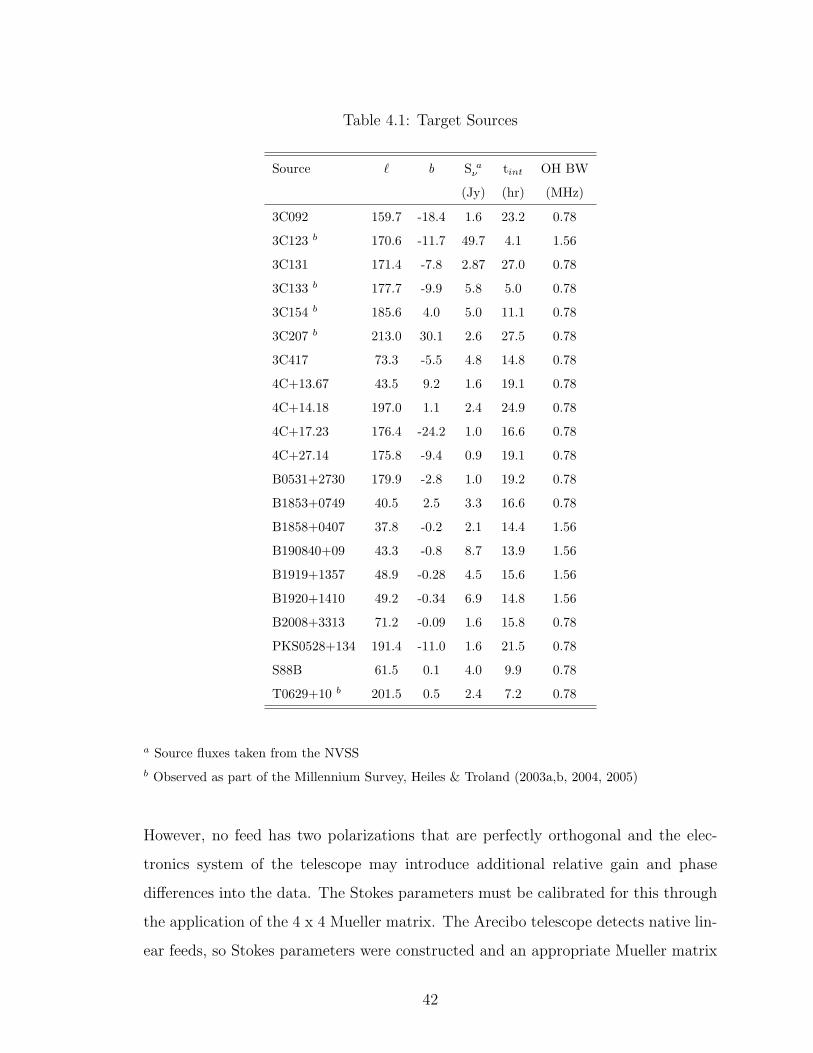
Table 4.1: Target Sources

Source ` b S aν tint OH BW

(Jy) (hr) (MHz)

3C092 159.7 -18.4 1.6 23.2 0.78

3C123 b 170.6 -11.7 49.7 4.1 1.56

3C131 171.4 -7.8 2.87 27.0 0.78

3C133 b 177.7 -9.9 5.8 5.0 0.78

3C154 b 185.6 4.0 5.0 11.1 0.78

3C207 b 213.0 30.1 2.6 27.5 0.78

3C417 73.3 -5.5 4.8 14.8 0.78

4C+13.67 43.5 9.2 1.6 19.1 0.78

4C+14.18 197.0 1.1 2.4 24.9 0.78

4C+17.23 176.4 -24.2 1.0 16.6 0.78

4C+27.14 175.8 -9.4 0.9 19.1 0.78

B0531+2730 179.9 -2.8 1.0 19.2 0.78

B1853+0749 40.5 2.5 3.3 16.6 0.78

B1858+0407 37.8 -0.2 2.1 14.4 1.56

B190840+09 43.3 -0.8 8.7 13.9 1.56

B1919+1357 48.9 -0.28 4.5 15.6 1.56

B1920+1410 49.2 -0.34 6.9 14.8 1.56

B2008+3313 71.2 -0.09 1.6 15.8 0.78

PKS0528+134 191.4 -11.0 1.6 21.5 0.78

S88B 61.5 0.1 4.0 9.9 0.78

T0629+10 b 201.5 0.5 2.4 7.2 0.78

a Source fluxes taken from the NVSSb Observed as part of the Millennium Survey, Heiles & Troland (2003a,b, 2004, 2005)

However, no feed has two polarizations that are perfectly orthogonal and the elec-

tronics system of the telescope may introduce additional relative gain and phase

differences into the data. The Stokes parameters must be calibrated for this through

the application of the 4 x 4 Mueller matrix. The Arecibo telescope detects native lin-

ear feeds, so Stokes parameters were constructed and an appropriate Mueller matrix

42

was applied to the data.

The reduction of Z16 HI data followed closely the method of Heiles & Troland

(2003a) used in the Millennium Survey. We wish to use absorption profiles to de-

termine the opacity and column density of HI for molecular clouds. Extracting the

absorption profiles in the direction of a continuum source can be problematic, espe-

cially in the case of HI. When pointing at a continuum source, absorption is only

sampled over the solid angle of the source, which is usually much smaller than the

beam. However, a radio telescope is sensitive to all radiation emanating from within

the beam and HI is widely spread throughout the Galaxy. Thus, the absorption spec-

trum is contaminated by emission in the vicinity of the source that often dominates

the spectrum. It is therefore possible to observe an emission spectrum while pointing

at a hot continuum source. In order to separate the emission and absorption contribu-

tions to the observed spectrum, one must have a way to sample only the HI emission

in the direction of the continuum source so it can be subtracted out. Ideally, one

would “turn off” the continuum source such that only emission would be present in

the source direction. However, since this is not possible, a series of off-source observa-

tions are used for this purpose. HI is known to have small scale spatial structure, so

a single pointing to one side of the continuum source will not likely yield an accurate

description of the HI in the direction of the continuum source. Therefore, a pattern of

16 off-source integrations are used to remove the first and second spatial derivatives

of HI structure and thus determine an accurate expected profile, the emission that

would be seen in the absence of the continuum source. See Section 3.1 for further

description of the Z16 pattern. The expected profile is combined with the opacity

profile to derive HI spin temperatures, as discussed in Section 4.7.2.

Observations of OH were primarily carried out using in-band frequency switching,

although a few Z16 patterns were included for the purpose of determining excitation

temperatures. Contrary to the Z16 observing pattern, frequency-switching does not

yield an off-source spectrum that is the result of pointing the telescope off of the

continuum source. The “on-source” signal and “off-source” reference spectra are

produced by shifting the center velocity of the band by approximately ± 14

of the

43

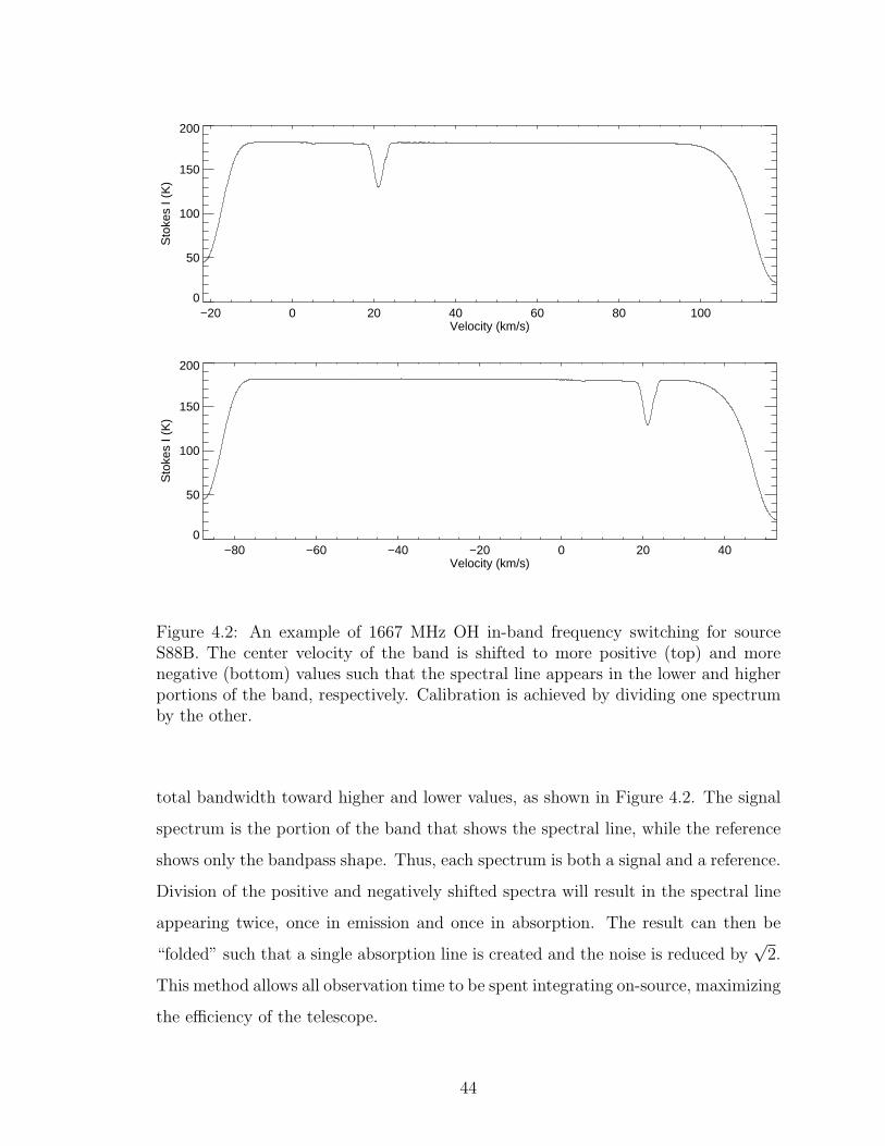
−20 0 20 40 60 80 100Velocity (km/s)

0

50

100

150

200

Sto

kes

I (K

)

−80 −60 −40 −20 0 20 40Velocity (km/s)

0

50

100

150

200

Sto

kes

I (K

)

Figure 4.2: An example of 1667 MHz OH in-band frequency switching for sourceS88B. The center velocity of the band is shifted to more positive (top) and morenegative (bottom) values such that the spectral line appears in the lower and higherportions of the band, respectively. Calibration is achieved by dividing one spectrumby the other.

total bandwidth toward higher and lower values, as shown in Figure 4.2. The signal

spectrum is the portion of the band that shows the spectral line, while the reference

shows only the bandpass shape. Thus, each spectrum is both a signal and a reference.

Division of the positive and negatively shifted spectra will result in the spectral line

appearing twice, once in emission and once in absorption. The result can then be

“folded” such that a single absorption line is created and the noise is reduced by√

2.

This method allows all observation time to be spent integrating on-source, maximizing

the efficiency of the telescope.

44

4.7 OH Results

This study comprises the first observational survey of the mass-to-flux ratio within

the lower density envelopes of molecular clouds. In this section, I present the results

of this survey.

4.7.1 Determination of Optical Depths

Opacity (e−τ ) spectra were constructed from the Stokes I data as described in Equa-

tion 2.7. The spectral line profiles in the direction of many target sources contain

several components which were often not well separated in velocity space. This is

especially true for those sources in the direction of the Galactic center. A separate

optical depth was obtained for each confused component by fitting the opacity profile

with a number of Gaussian components. The optical depth of each velocity compo-

nent could then be determined from the height of the fit Gaussian. Individual results

were obtained for the 1665 and 1667 MHz OH transitions.

For optically thin gas in LTE, it is expected that the relative optical depths of

the 1665 and 1667 MHz OH lines is 5:9. That is, τ1667 = (9/5) τ1665. This ratio is

highly sensitive the physical environment and deviations from the expected value can

be an indication that non-thermal processes are dominate in the region. Moreover, it

is possible in some cases that τ1665 > τ1667, a scenario called the main-line anomaly. If

such an anomaly exists or the optical depth ratio deviates far from the expected value,

the sampled environment may not well represent the general envelopes of GMCs.

We find the ratio τ1667/τ1665 ≈ 1.8 for most of our lines of sight, with an average

value of 1.9 for the ensemble. There are, however, a few individual velocity compo-

nents for which the ratio is much higher than the expected value. Careful inspection

of the Stokes V profiles for these suspect components revealed features characterisic

of masing. Such components are expected to be associated with HII regions and were

therefore discarded from our sample. Optical depths for the 1665 and 1667 MHz tran-

sitions can be found in columns (4) and (5) of Table 4.2.

45

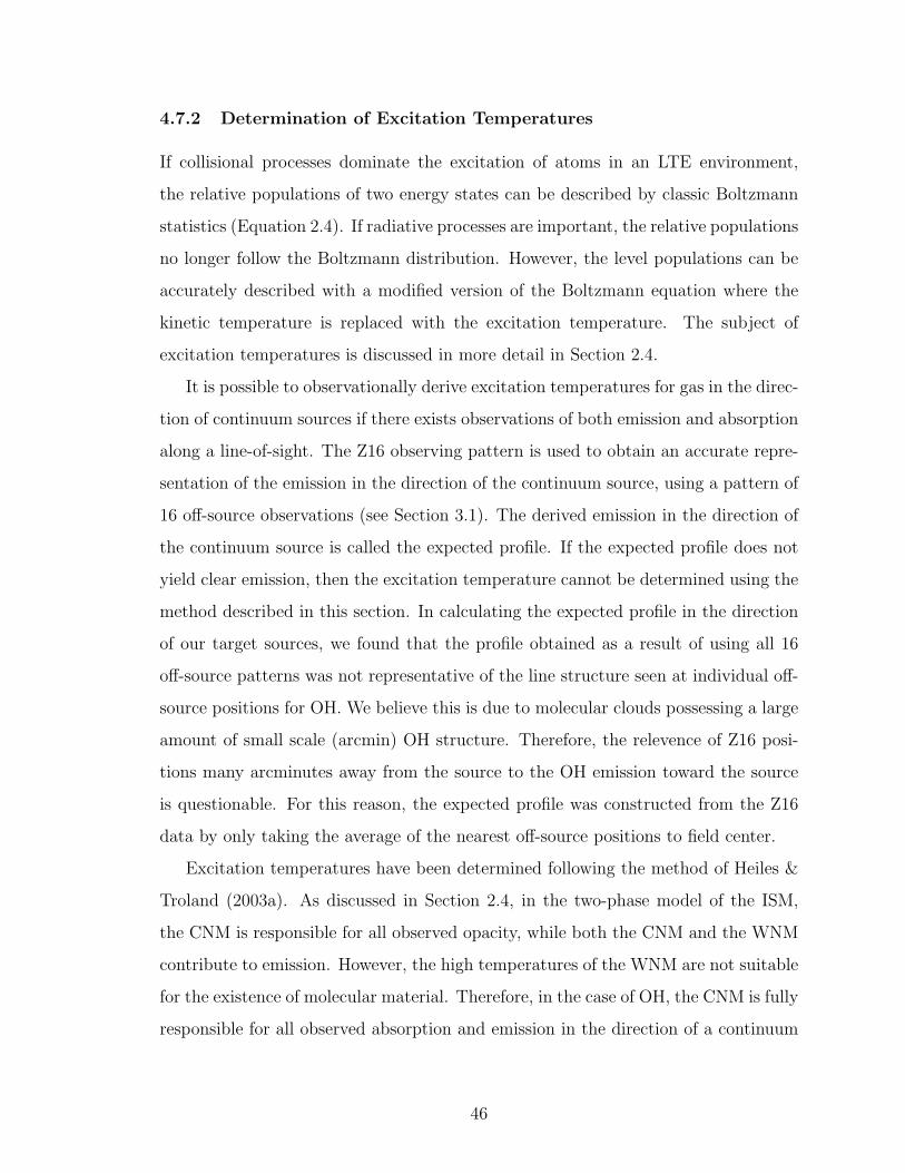
4.7.2 Determination of Excitation Temperatures

If collisional processes dominate the excitation of atoms in an LTE environment,

the relative populations of two energy states can be described by classic Boltzmann

statistics (Equation 2.4). If radiative processes are important, the relative populations

no longer follow the Boltzmann distribution. However, the level populations can be

accurately described with a modified version of the Boltzmann equation where the

kinetic temperature is replaced with the excitation temperature. The subject of

excitation temperatures is discussed in more detail in Section 2.4.

It is possible to observationally derive excitation temperatures for gas in the direc-

tion of continuum sources if there exists observations of both emission and absorption

along a line-of-sight. The Z16 observing pattern is used to obtain an accurate repre-

sentation of the emission in the direction of the continuum source, using a pattern of

16 off-source observations (see Section 3.1). The derived emission in the direction of

the continuum source is called the expected profile. If the expected profile does not

yield clear emission, then the excitation temperature cannot be determined using the

method described in this section. In calculating the expected profile in the direction

of our target sources, we found that the profile obtained as a result of using all 16

off-source patterns was not representative of the line structure seen at individual off-

source positions for OH. We believe this is due to molecular clouds possessing a large

amount of small scale (arcmin) OH structure. Therefore, the relevence of Z16 posi-

tions many arcminutes away from the source to the OH emission toward the source

is questionable. For this reason, the expected profile was constructed from the Z16

data by only taking the average of the nearest off-source positions to field center.

Excitation temperatures have been determined following the method of Heiles &

Troland (2003a). As discussed in Section 2.4, in the two-phase model of the ISM,

the CNM is responsible for all observed opacity, while both the CNM and the WNM

contribute to emission. However, the high temperatures of the WNM are not suitable

for the existence of molecular material. Therefore, in the case of OH, the CNM is fully

responsible for all observed absorption and emission in the direction of a continuum

46

source. To determine Tex, we first represent the opacity profile by a collection of

Gaussians by performing a least-squares fit, yielding individual values of the optical

depth, center frequency, and Gaussian width for each component. We then perform a

least-squares Gaussian fit to the expected emission profile. We require the fit Gaussian

components to possess the same center frequencies and Gaussian widths as derived

from the opacity profile fit, but allow the Gaussian heights to vary. This ensures that

the same CNM components responsible for absorption are providing the brightness

temperature in the emission profile. The excitation temperature for each component

is then proportional to the derived Gaussian height from the expected profile fit.

Derived excitation temperatures for both 1665 and 1667 MHz OH lines are pre-

sented in columns (6) and (7) of Table 4.2. The expected profile did not reveal OH

emission in the direction of all continuum sources, so Tex could only be determined for

a subset of our lines-of-sight. The values in the table containing errors are the com-

ponents for which the temperature could be determined by the least-squares fitting

techinque. Values listed without error are the directions in which off-source emission

was not observed, and Tex is assumed to be the average of the derived values for the

particular frequency. We find Tex ∼ 9 - 10 K for both the 1665 and 1667 MHz tran-

sitions.

Table 4.2: OH Main Line Optical Depth and Excitation Temperature Results

Source V alsr ∆V a τ65 τ67 Tex,65 Tex,67

(km s−1) (km s−1) (K) (K)

3C092 8.8 ± 0.0 0.88 ± 0.02 0.073 ± 0.001 0.111 ± 0.001 9.1 ± 0.6 10.5 ± 0.4

3C123 5.5 ± 0.0 0.90 ± 0.02 0.034 ± 0.001 0.079 ± 0.001 9.0 10.0

4.5 ± 0.0 0.56 ± 0.01 0.039 ± 0.001 0.091 ± 0.001 9.0 10.0

3.7 ± 0.0 1.40 ± 0.03 0.020 ± 0.001 0.036 ± 0.001 9.0 10.0

3C131 7.2 ± 0.0 0.59 ± 0.02 0.059 ± 0.001 0.094 ± 0.001 10.1 ± 0.5 10.1 ± 0.3

6.6 ± 0.0 0.52 ± 0.04 0.023 ± 0.001 0.034 ± 0.001 9.8 ± 1.3 10.3 ± 1.0

4.6 ± 0.0 0.85 ± 0.06 0.007 ± 0.000 0.030 ± 0.001 13.8 ± 3.1 13.5 ± 1.8

3C133 7.7 ± 0.0 0.60 ± 0.01 0.093 ± 0.001 0.194 ± 0.002 9.0 10.0

Continued on Next Page. . .

47

Table 4.2 – Continued

Source V alsr ∆V a τ65 τ67 Tex,65 Tex,67

3C154 -2.3 ± 0.0 0.73 ± 0.04 0.025 ± 0.001 0.040 ± 0.001 9.0 10.0

3C207 4.6 ± 0.0 0.78 ± 0.02 0.015 ± 0.000 0.027 ± 0.000 9.0 10.0

3C417 9.8 ± 0.0 0.99 ± 0.03 0.104 ± 0.003 0.189 ± 0.004 8.6 ± 0.5 8.70 ± 0.3

4C+13.67 5.4 ± 0.1 0.61 ± 0.18 0.025 ± 0.003 0.027 ± 0.007 9.0 10.0

4.7 ± 0.1 0.59 ± 0.10 0.047 ± 0.008 0.031 ± 0.006 9.0 10.0

4C+14.18 32.0 ± 0.0 0.42 ± 0.03 0.020 ± 0.001 0.038 ± 0.002 9.0 10.0

4C+17.23 11.2 ± 0.0 0.76 ± 0.07 0.032 ± 0.003 0.053 ± 0.003 9.0 10.0

9.2 ± 0.0 0.68 ± 0.08 0.028 ± 0.003 0.054 ± 0.004 9.0 10.0

B0531+2730 2.9 ± 0.0 0.76 ± 0.04 0.060 ± 0.003 0.120 ± 0.004 9.0 10.0

B1853+0749 28.2 ± 0.0 1.48 ± 0.06 0.108 ± 0.003 0.228 ± 0.008 10.7 ± 1.1 8.7 ± 0.5

26.7 ± 0.1 1.72 ± 0.09 0.050 ± 0.002 0.178 ± 0.008 12.4 ± 1.8 10.9 ± 0.5

8.1 ± 0.0 0.85 ± 0.05 0.040 ± 0.003 0.093 ± 0.002 6.2 ± 2.8 11.1 ± 1.2

B1858+0407 20.4 ± 0.0 0.71 ± 0.08 0.065 ± 0.009 0.107 ± 0.008 3.2 ± 4.8 8.3 ± 3.6

19.4 ± 0.1 2.00 ± 0.35 0.031 ± 0.003 0.088 ± 0.004 12.5 ± 6.3 2.3 ± 2.5

16.9 ± 0.1 1.25 ± 0.24 0.033 ± 0.004 0.060 ± 0.005 10.0 ± 7.2 7.2 ± 9.3

15.0 ± 0.1 1.47 ± 0.38 0.035 ± 0.004 0.080 ± 0.005 5.0 ± 6.1 1.1 ± 2.9

13.6 ± 0.1 1.24 ± 0.11 0.082 ± 0.008 0.090 ± 0.006 6.5 ± 3.1 7.8 ± 1.4

B190840+09 43.3 ± 0.0 1.22 ± 0.11 0.030 ± 0.002 0.043 ± 0.003 9.0 10.0

40.5 ± 0.0 2.30 ± 0.09 0.072 ± 0.003 0.085 ± 0.004 9.0 10.0

B1919+1357 6.4 ± 0.1 1.34 ± 0.07 0.068 ± 0.006 0.168 ± 0.002 9.0 10.0

B1920+1410 6.3 ± 0.0 1.30 ± 0.33 0.035 ± 0.014 0.087 ± 0.002 9.0 10.0

5.1 ± 0.0 0.65 ± 0.35 0.021 ± 0.019 0.048 ± 0.003 9.0 10.0

B2008+3313 11.3 ± 0.0 0.77 ± 0.04 0.062 ± 0.004 0.122 ± 0.004 8.5 ± 2.3 11.5 ± 1.2

9.2 ± 0.0 1.60 ± 0.07 0.055 ± 0.003 0.104 ± 0.003 9.5 ± 1.8 12.0 ± 1.0

PKS0528+134 9.6 ± 0.0 0.91 ± 0.04 0.025 ± 0.001 0.046 ± 0.001 9.0 10.0

S88B 21.3 ± 0.0 2.57 ± 0.01 0.466 ± 0.002 0.541 ± 0.003 10.5 ± 0.1 10.5 ± 0.1

T0629+10 6.9 ± 0.0 0.62 ± 0.10 0.044 ± 0.003 0.077 ± 0.005 9.0 10.0

6.1 ± 0.0 0.72 ± 0.10 0.079 ± 0.003 0.125 ± 0.005 9.0 10.0

4.6 ± 0.0 0.54 ± 0.04 0.085 ± 0.003 0.156 ± 0.005 9.0 10.0

2.9 ± 0.0 0.82 ± 0.02 0.172 ± 0.003 0.262 ± 0.005 9.0 10.0

a Center velocities and FWHM line widths are 1665 and 1667 MHz averages.

48

4.7.3 Magnetic Field Strengths

The majority of our line profiles are complicated and often consist of several confused

velocity components. Therefore, to determine magnetic field strengths, the Stokes I

spectral line was represented by a combination of Gaussian components. One of

the challenges of fitting multiple Gaussians to complicated spectral lines is choosing

how many Gaussians to fit. As the number of Gaussian components increase, the

goodness-of-fit will also increase, but each Gaussian parameter is known with less

certainty. Therefore, one must exercise restraint when performing Gaussian decom-

position. The number of Gaussian components fit to Stokes I was chosen such that

only the main features of the line clearly distinguishable from random noise were fit.

Magnetic field strengths were derived using Equation 2.3: the derivative of the

resultant noise-free Gaussian was fit to the Stokes V profile via a linear least-squares

fitting technique. As discussed in Section 2.1, the Zeeman effect reveals itself in

the Stokes V profile as a scaled version of the derivative of the Stokes I spectrum.

The scaling factor, which is revealed by the least-squares fit, is proportional to the

strength of the magnetic field. The use of several Gaussians to represent the Stokes I

profile allows for the calculation of a separate field strength for each individual veloc-

ity component. Since each velocity component represents the motion of a different

molecular cloud encountered along the line-of-sight, a single telescope pointing can

reveal magnetic field information for several different clouds. This is especially true

for low latitude sources where the profiles are usually complicated and HI absorption

may appear over several hundred kilometers per second.

Magnetic field strengths were determined independently for the 1665 and 1667 MHz

OH lines using the combined Z16 and in-band frequency switching data. A single field

was computed by taking the average of the two measurements, weighted by the inverse

square of the 1σ uncertainty in the field, resulting in a√

2 reduction in noise. Mag-

netic field fitting results can be found in Table 4.3. In this table, column (1) gives the

source name, column (2) the velocity of the OH Gaussian component, column (3) the

49

magnetic field strength and direction as determined from the 1665 MHz line with its

1σ uncertainty, column (4) is the same as column (3) but for the 1667 MHz OH line,

column (5) is the weighted mean line-of-sight field for the two OH main lines and

the weighted 1σ uncertainty, column (6) is the HI column density, and column (7) is

the calculated mass-to-flux ratio. The determination of N and λ will be discussed in

later sections. Only Gaussian components that satisfy the following criteria were in-

cluded in the table and used for subsequent analysis: the uncertainty in Blos, σB, was

less than 20 µG, the 1665 and 1667 MHz measurements agree within error (|B1665 -

B1667| < σB), and the Stokes V profile was well fit by the derivative of the Gaussian

representation dI/dν.

We report Zeeman detections in a total of 5 velocity components belonging to lines-

of-sight toward 3C092, 3C133, 4C+13.67, B1858+0407, and S88B. We also report

potential detections in 4 components toward B1853+0749, 3C123, and 3C154. Field

strengths for the detections are in bold face in Table 4.3. In order for the magnetic

field strength to be considered a detection, we require that the measured field strength

be greater than 3 times the uncertainty (Blos > 3σB) and the plot of Stokes V look

consistent with detection of the Zeeman effect. The 4 components with possible

detections satisfy criterion 1, but not 2. It is important to note that for our survey

of mass-to-flux ratios detections are not required, only sensitive upper limits to the

field strength. Sensitive upper limits on the field yield lower limits to λ. If we find

lower limits such that λ > 1, then we can conclude that molecular cloud envelopes

are not subcritical. Figure 4.3 shows an example of the 1665 and 1667 MHz profiles

for 3C092, a source with a clear Zeeman detection. The top panel shows the Stokes I

profile (I = RR + LL) and the bottom panel shows the Stokes V profile (V = RR - LL,

histogram) and the least-squares fit (smooth line). A single Gaussian component was

fit to the Stokes I spectrum. Zeeman analysis yielded a field of Blos = -15.5 ± 2.8 µG,

the negative sign indicating the field is oriented toward the observer. Similar plots

for all lines-of-sight included in this study can be found in Appendix A: Molecular

Cloud OH Spectra and Magnetic Field Fitting.

Our results for field strengths are consistent with, and improve upon, previous

50

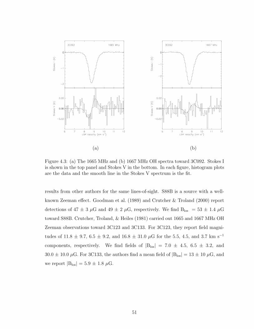
(a) (b)

Figure 4.3: (a) The 1665 MHz and (b) 1667 MHz OH spectra toward 3C092. Stokes Iis shown in the top panel and Stokes V in the bottom. In each figure, histogram plotsare the data and the smooth line in the Stokes V spectrum is the fit.

results from other authors for the same lines-of-sight. S88B is a source with a well-

known Zeeman effect. Goodman et al. (1989) and Crutcher & Troland (2000) report

detections of 47 ± 3 µG and 49 ± 2 µG, respectively. We find Blos = 53 ± 1.4 µG

toward S88B. Crutcher, Troland, & Heiles (1981) carried out 1665 and 1667 MHz OH

Zeeman observations toward 3C123 and 3C133. For 3C123, they report field magni-

tudes of 11.8 ± 9.7, 6.5 ± 9.2, and 16.8 ± 31.0 µG for the 5.5, 4.5, and 3.7 km s−1

components, respectively. We find fields of |Blos| = 7.0 ± 4.5, 6.5 ± 3.2, and

30.0 ± 10.0 µG. For 3C133, the authors find a mean field of |Blos| = 13 ± 10 µG, and

we report |Blos| = 5.9 ± 1.8 µG.

51

4.7.4 Determination of Column Densities

The column density of OH is derived assuming the the lines are optically thin via

N(OH) = C Tex

∫τν dν cm−2, (4.1)

where the constant C = 4.1063 x 1014 and 2.2785 x 1014 cm−2 (km s−1)−1 for the

1665 and 1667 MHz OH lines, respectively, τν is the frequency dependent optical

depth, and Tex is the excitation temperature (Roberts, 1995). The dominate source

of uncertainty in this calculation is the excitation temperature. However, we expect

our derived values to be accurate within a few degrees.

We infer hydrogen column density toward each target source using the OH abun-

dance ratio given by Crutcher (1979) of N(OH)/N(H) = 4 × 10−8, which is uncertain

by a factor of approximately 2. This ratio was derived by calculating the normal-

ized column density N(OH)/Av for lines-of-sight with known visual extinctions. The

abundance of OH was then determined by using the well-known ratio for N(H)/AV,

given in Equation 2.11. In the ratio, N(H) = N(HI) + 2N(H2) is the total hydrogen

column density.

Column densities for each velocity component were determined separately for the

1665 and 1667 MHz OH transitions. The hydrogen column density calculated from

the average of the two OH lines is given in column (6) of Table 4.3.

4.7.5 Calculation of Mass-to-Flux Ratios

As discussed in Section 2.8, the mass-to-flux ratio can be calculated via

λ = 5.0× 10−21 N(H)

|B|,

where N(H) is the total hydrogen column density. A value of λ = 1 is the critical

ratio, for which the gravitational and magnetic energies are equal. If λ > 1, gravity

dominates magnetic energy, and the cloud is said to be magnetically supercritical. On

the other hand, if λ < 1, then the magnetic energy alone is sufficient to support the

cloud against gravitational collapse, and the cloud is magnetically subcritical.

52

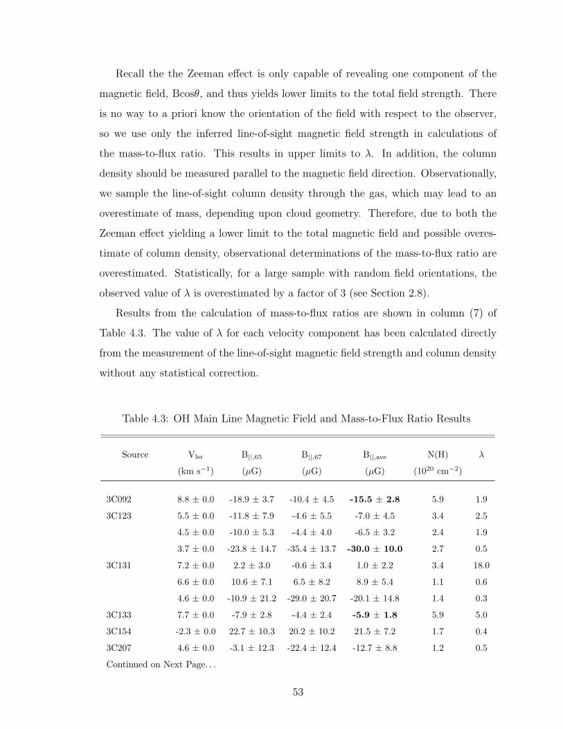
Recall the the Zeeman effect is only capable of revealing one component of the

magnetic field, Bcosθ, and thus yields lower limits to the total field strength. There

is no way to a priori know the orientation of the field with respect to the observer,

so we use only the inferred line-of-sight magnetic field strength in calculations of

the mass-to-flux ratio. This results in upper limits to λ. In addition, the column

density should be measured parallel to the magnetic field direction. Observationally,

we sample the line-of-sight column density through the gas, which may lead to an

overestimate of mass, depending upon cloud geometry. Therefore, due to both the

Zeeman effect yielding a lower limit to the total magnetic field and possible overes-

timate of column density, observational determinations of the mass-to-flux ratio are

overestimated. Statistically, for a large sample with random field orientations, the

observed value of λ is overestimated by a factor of 3 (see Section 2.8).

Results from the calculation of mass-to-flux ratios are shown in column (7) of

Table 4.3. The value of λ for each velocity component has been calculated directly

from the measurement of the line-of-sight magnetic field strength and column density

without any statistical correction.

Table 4.3: OH Main Line Magnetic Field and Mass-to-Flux Ratio Results

Source Vlsr B||,65 B||,67 B||,ave N(H) λ

(km s−1) (µG) (µG) (µG) (1020 cm−2)

3C092 8.8 ± 0.0 -18.9 ± 3.7 -10.4 ± 4.5 -15.5 ± 2.8 5.9 1.9

3C123 5.5 ± 0.0 -11.8 ± 7.9 -4.6 ± 5.5 -7.0 ± 4.5 3.4 2.5

4.5 ± 0.0 -10.0 ± 5.3 -4.4 ± 4.0 -6.5 ± 3.2 2.4 1.9

3.7 ± 0.0 -23.8 ± 14.7 -35.4 ± 13.7 -30.0 ± 10.0 2.7 0.5

3C131 7.2 ± 0.0 2.2 ± 3.0 -0.6 ± 3.4 1.0 ± 2.2 3.4 18.0

6.6 ± 0.0 10.6 ± 7.1 6.5 ± 8.2 8.9 ± 5.4 1.1 0.6

4.6 ± 0.0 -10.9 ± 21.2 -29.0 ± 20.7 -20.1 ± 14.8 1.4 0.3

3C133 7.7 ± 0.0 -7.9 ± 2.8 -4.4 ± 2.4 -5.9 ± 1.8 5.9 5.0

3C154 -2.3 ± 0.0 22.7 ± 10.3 20.2 ± 10.2 21.5 ± 7.2 1.7 0.4

3C207 4.6 ± 0.0 -3.1 ± 12.3 -22.4 ± 12.4 -12.7 ± 8.8 1.2 0.5

Continued on Next Page. . .

53

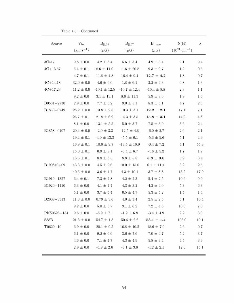
Table 4.3 – Continued

Source Vlsr B||,65 B||,67 B||,ave N(H) λ

(km s−1) (µG) (µG) (µG) (1021 cm−2)

3C417 9.8 ± 0.0 4.2 ± 3.4 5.6 ± 3.4 4.9 ± 3.4 9.1 9.4

4C+13.67 5.4 ± 0.1 8.6 ± 11.0 11.6 ± 20.8 9.3 ± 9.7 1.2 0.6

4.7 ± 0.1 11.8 ± 4.8 16.4 ± 9.4 12.7 ± 4.2 1.8 0.7

4C+14.18 32.0 ± 0.0 4.6 ± 6.0 1.8 ± 6.1 3.2 ± 4.3 0.8 1.3

4C+17.23 11.2 ± 0.0 -10.1 ± 12.5 -10.7 ± 12.4 -10.4 ± 8.8 2.3 1.1

9.2 ± 0.0 3.1 ± 13.1 8.0 ± 11.3 5.9 ± 8.6 1.9 1.6

B0531+2730 2.9 ± 0.0 7.7 ± 5.2 9.0 ± 5.1 8.3 ± 5.1 4.7 2.8

B1853+0749 28.2 ± 0.0 13.8 ± 2.8 10.3 ± 3.1 12.2 ± 2.1 17.1 7.1

26.7 ± 0.1 21.8 ± 6.9 14.3 ± 3.5 15.8 ± 3.1 14.9 4.8

8.1 ± 0.0 13.1 ± 5.5 5.0 ± 3.7 7.5 ± 3.0 3.6 2.4

B1858+0407 20.4 ± 0.0 -2.9 ± 3.3 -12.5 ± 4.8 -6.0 ± 2.7 2.6 2.1

19.4 ± 0.1 -4.0 ± 13.3 -5.5 ± 6.1 -5.3 ± 5.6 5.1 4.9

16.9 ± 0.1 10.0 ± 9.7 -13.5 ± 10.9 -0.4 ± 7.2 4.1 55.3

15.0 ± 0.1 0.9 ± 8.1 -8.4 ± 6.7 -4.6 ± 5.2 1.7 1.9

13.6 ± 0.1 8.8 ± 3.5 8.8 ± 5.8 8.8 ± 3.0 5.9 3.4

B190840+09 43.3 ± 0.0 4.5 ± 9.6 10.0 ± 15.0 6.1 ± 11.4 3.2 2.6

40.5 ± 0.0 3.6 ± 4.7 4.3 ± 10.1 3.7 ± 8.8 13.2 17.9

B1919+1357 6.4 ± 0.1 7.3 ± 2.8 4.2 ± 2.3 5.4 ± 2.5 10.6 9.9

B1920+1410 6.3 ± 0.0 4.1 ± 4.4 4.3 ± 3.2 4.2 ± 4.0 5.3 6.3

5.1 ± 0.0 3.7 ± 5.4 6.5 ± 4.7 5.3 ± 5.2 1.5 1.4

B2008+3313 11.3 ± 0.0 0.79 ± 3.6 4.0 ± 3.4 2.5 ± 2.5 5.1 10.4

9.2 ± 0.0 5.0 ± 6.7 9.1 ± 6.2 7.2 ± 4.6 10.0 7.0

PKS0528+134 9.6 ± 0.0 -5.9 ± 7.1 -1.2 ± 6.8 -3.4 ± 4.9 2.2 3.3

S88B 21.3 ± 0.0 54.7 ± 1.8 50.6 ± 2.2 53.1 ± 1.4 106.0 10.1

T0629+10 6.9 ± 0.0 20.1 ± 9.5 16.8 ± 10.5 18.6 ± 7.0 2.6 0.7

6.1 ± 0.0 9.2 ± 6.0 3.6 ± 7.6 7.0 ± 4.7 5.2 3.7

4.6 ± 0.0 7.1 ± 4.7 4.3 ± 4.9 5.8 ± 3.4 4.5 3.9

2.9 ± 0.0 -4.8 ± 2.6 -3.1 ± 3.6 -4.2 ± 2.1 12.6 15.1

54

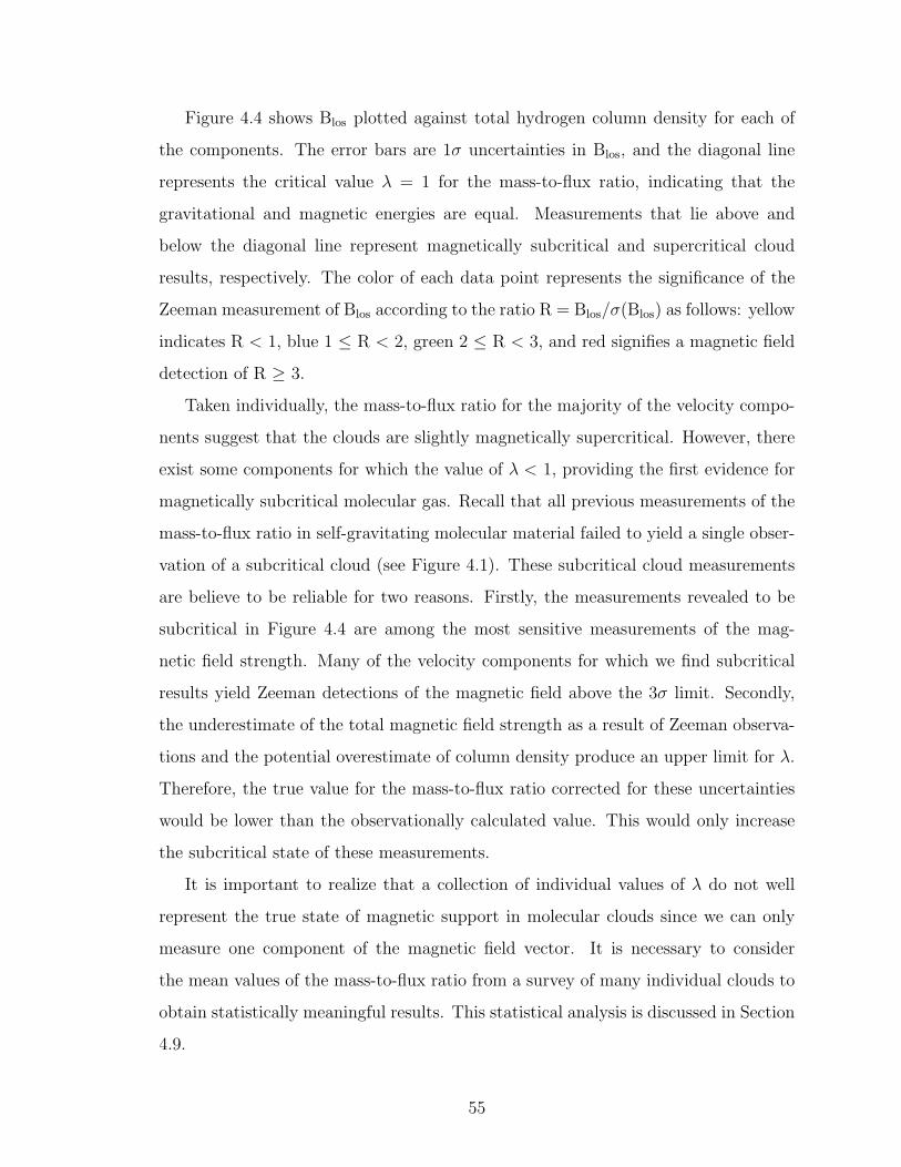
Figure 4.4 shows Blos plotted against total hydrogen column density for each of

the components. The error bars are 1σ uncertainties in Blos, and the diagonal line

represents the critical value λ = 1 for the mass-to-flux ratio, indicating that the

gravitational and magnetic energies are equal. Measurements that lie above and

below the diagonal line represent magnetically subcritical and supercritical cloud

results, respectively. The color of each data point represents the significance of the

Zeeman measurement of Blos according to the ratio R = Blos/σ(Blos) as follows: yellow

indicates R < 1, blue 1 ≤ R < 2, green 2 ≤ R < 3, and red signifies a magnetic field

detection of R ≥ 3.

Taken individually, the mass-to-flux ratio for the majority of the velocity compo-

nents suggest that the clouds are slightly magnetically supercritical. However, there

exist some components for which the value of λ < 1, providing the first evidence for

magnetically subcritical molecular gas. Recall that all previous measurements of the

mass-to-flux ratio in self-gravitating molecular material failed to yield a single obser-

vation of a subcritical cloud (see Figure 4.1). These subcritical cloud measurements

are believe to be reliable for two reasons. Firstly, the measurements revealed to be

subcritical in Figure 4.4 are among the most sensitive measurements of the mag-

netic field strength. Many of the velocity components for which we find subcritical

results yield Zeeman detections of the magnetic field above the 3σ limit. Secondly,

the underestimate of the total magnetic field strength as a result of Zeeman observa-

tions and the potential overestimate of column density produce an upper limit for λ.

Therefore, the true value for the mass-to-flux ratio corrected for these uncertainties

would be lower than the observationally calculated value. This would only increase

the subcritical state of these measurements.

It is important to realize that a collection of individual values of λ do not well

represent the true state of magnetic support in molecular clouds since we can only

measure one component of the magnetic field vector. It is necessary to consider

the mean values of the mass-to-flux ratio from a survey of many individual clouds to

obtain statistically meaningful results. This statistical analysis is discussed in Section

4.9.

55

Blos vs NH

1020 1021 1022 1023

NH (cm−2)

0.1

1.0

10.0

100.0

1000.0B

los

(µG

)

Figure 4.4: Results for the mass-to-flux ratio in molecular clouds observed with OH.These results reflect λ in the general regions of molecular clouds, not specifically inthe cores. The diagonal line indicates the critical ratio for which the gravitational andmagnetic influences are equal. Measurements above the line are subcritical (magnet-ically dominated), those below are supercritical (gravitationally dominated). Errorbars are 1 sigma uncertainties in Blos. The significance of each Blos measurement isindicated by color as follows: yellow indicates B/σ(B) < 1, blue 1 ≤ B/σ(B) < 2,green 2 ≤ B/σ(B) < 3, and red signifies a magnetic field detection of B/σ(B) ≥ 3.

Figure 4.5 shows the collection of all mass-to-flux ratio results. Previous results

discussed in Section 4.2 and presented in Figure 4.1 are shown in black, and the

results of the current study in red. The black measurements from previous studies

contain results for HI CNM diffuse clouds (N(H) < ∼ 1.5 × 1021), and molecular

cores observed in OH (1.5 × 1021 < N(H) < 5 × 1022) and CN (N(H) < 5 × 1022).

The results of the current study are the first such measurements of the mass-to-flux

ratio in molecular clouds as a whole, not specifically in molecular cores. The diagonal

56

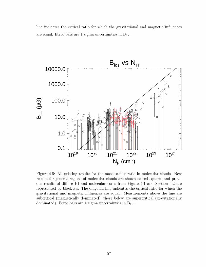
line indicates the critical ratio for which the gravitational and magnetic influences

are equal. Error bars are 1 sigma uncertainties in Blos.

Blos vs NH

1019 1020 1021 1022 1023 1024

NH (cm−2)

0.1

1.0

10.0

100.0

1000.0

10000.0

Blo

s (µ

G)

Figure 4.5: All existing results for the mass-to-flux ratio in molecular clouds. Newresults for general regions of molecular clouds are shown as red squares and previ-ous results of diffuse HI and molecular cores from Figure 4.1 and Section 4.2 arerepresented by black x’s. The diagonal line indicates the critical ratio for which thegravitational and magnetic influences are equal. Measurements above the line aresubcritical (magnetically dominated), those below are supercritical (gravitationallydominated). Error bars are 1 sigma uncertainties in Blos.

57

4.8 HI Results

For HI, the excitation temperature assumes the name spin temperature to reflect

the fact that it represents the relative level populations in the spin-flip transition of

neutral hydrogen. The determination of the spin temperature proceeds differently

from that of the OH excitation temperature. In the case of OH, the CNM is solely

responsible for both the emission and absorption in the direction of a background

continuum source since molecular species are unable to survive in the high temper-

atures of the WNM. This is not true for atomic species. The CNM alone provides

the HI opacity, but both the CNM and WNM contribute to the observed emission.

Therefore, the WNM cannot be ignored as in Section 4.7.2.

The least-squares Gaussian fitting of the opacity profile proceeds exactly as de-

scribed for OH excitation temperatures. Having fit Gaussian components to the

opacity profile, we then fit the expected emission profile to the sum of the emission

contribution from the CNM and WNM. The centers and widths of the CNM opac-

ity Gaussians are once again held constant, and the heights are allowed to vary. A

number of additional Gaussians are added to the set of CNM components to describe

the WNM contribution to the emission. The excitation temperature can then be

determined through a least-squares fit of the collection of CNM and WNM Gaussian

components to the expected emission profile.

The HI column density for each component can be calculated with knowledge of

the optical depth, spin temperature, and FWHM velocity width of the the line by

N(HI)CNM = 1.95× 1018 τ0 TS ∆VFWHM cm−2, and

N(HI)WNM = 4.2× 1017 τ0 TS Tk,max1/2 cm−2

for CNM and WNM components, where τ0 is optical depth at the line peak and TS

is the spin temperature (Heiles & Troland, 2003b).

The Gaussian parameters for each fit CNM and WNM component, as well as the

HI spin temperature and column density results, can be found in Table 4.4. For a few

CNM components, the value of TS had to be forced to zero for the fit of the expected

profile to converge. For these components, the column density was also set to 0.

58

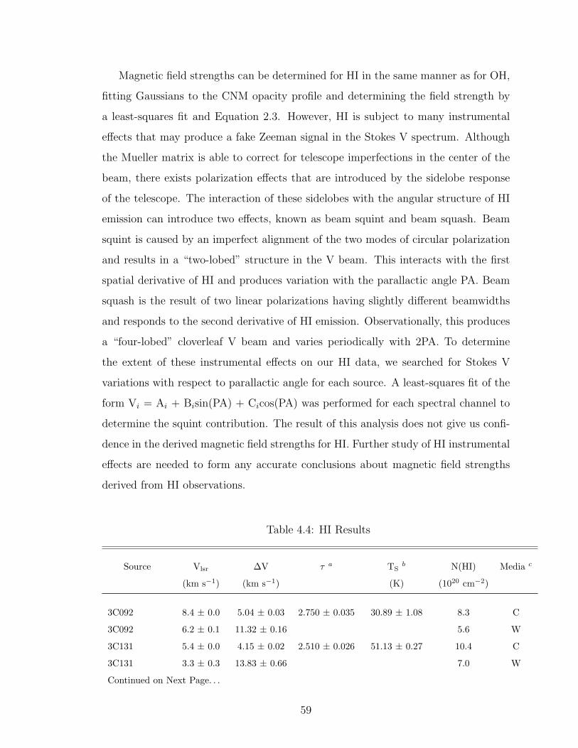
Magnetic field strengths can be determined for HI in the same manner as for OH,

fitting Gaussians to the CNM opacity profile and determining the field strength by

a least-squares fit and Equation 2.3. However, HI is subject to many instrumental

effects that may produce a fake Zeeman signal in the Stokes V spectrum. Although

the Mueller matrix is able to correct for telescope imperfections in the center of the

beam, there exists polarization effects that are introduced by the sidelobe response

of the telescope. The interaction of these sidelobes with the angular structure of HI

emission can introduce two effects, known as beam squint and beam squash. Beam

squint is caused by an imperfect alignment of the two modes of circular polarization

and results in a “two-lobed” structure in the V beam. This interacts with the first

spatial derivative of HI and produces variation with the parallactic angle PA. Beam

squash is the result of two linear polarizations having slightly different beamwidths

and responds to the second derivative of HI emission. Observationally, this produces

a “four-lobed” cloverleaf V beam and varies periodically with 2PA. To determine

the extent of these instrumental effects on our HI data, we searched for Stokes V

variations with respect to parallactic angle for each source. A least-squares fit of the

form Vi = Ai + Bisin(PA) + Cicos(PA) was performed for each spectral channel to

determine the squint contribution. The result of this analysis does not give us confi-

dence in the derived magnetic field strengths for HI. Further study of HI instrumental

effects are needed to form any accurate conclusions about magnetic field strengths

derived from HI observations.

Table 4.4: HI Results

Source Vlsr ∆V τ a TSb N(HI) Media c

(km s−1) (km s−1) (K) (1020 cm−2)

3C092 8.4 ± 0.0 5.04 ± 0.03 2.750 ± 0.035 30.89 ± 1.08 8.3 C

3C092 6.2 ± 0.1 11.32 ± 0.16 5.6 W

3C131 5.4 ± 0.0 4.15 ± 0.02 2.510 ± 0.026 51.13 ± 0.27 10.4 C

3C131 3.3 ± 0.3 13.83 ± 0.66 7.0 W

Continued on Next Page. . .

59

Table 4.4 – Continued

Source Vlsr ∆V τ a TSb N(HI) Media c

(km s−1) (km s−1) (K) (1020 cm−2)

3C131 -2.1 ± 0.0 7.02 ± 0.12 0.360 ± 0.004 98.93 ± 2.81 4.8 C

3C131 -12.4 ± 1.7 26.74 ± 3.02 5.8 W

3C131 -37.8 ± 0.1 1.47 ± 0.28 0.081 ± 0.021 0.00 ± 0.00 0.0 C

3C131 -39.0 ± 0.2 11.34 ± 0.49 2.0 W

3C131 -39.7 ± 0.2 3.01 ± 0.40 0.109 ± 0.006 87.88 ± 5.01 0.6 C

3C417 15.4 ± 0.0 4.11 ± 0.14 0.501 ± 0.015 87.55 ± 1.44 3.5 C

3C417 13.0 ± 0.1 2.81 ± 0.15 0.9 W

3C417 10.4 ± 0.0 3.13 ± 0.04 1.750 ± 0.030 65.92 ± 0.67 7.0 C

3C417 8.6 ± 0.4 12.62 ± 0.44 0.201 ± 0.010 165.56 ± 2.44 8.2 C

3C417 2.3 ± 0.2 36.14 ± 0.47 10.0 W

3C417 -8.5 ± 0.1 2.63 ± 0.24 0.082 ± 0.007 0.00 ± 0.00 0.0 C

4C+13.67 20.7 ± 0.3 16.61 ± 1.39 2.8 W

4C+13.67 6.5 ± 0.0 4.39 ± 0.05 0.870 ± 0.100 47.59 ± 1.03 3.5 C

4C+13.67 4.4 ± 0.1 9.90 ± 0.20 3.0 W

4C+13.67 2.0 ± 0.0 2.04 ± 0.03 1.070 ± 0.017 34.85 ± 0.85 1.5 C

4C+14.18 32.6 ± 0.0 3.12 ± 0.06 0.640 ± 0.010 67.30 ± 1.04 2.6 C

4C+14.18 29.0 ± 0.1 2.14 ± 0.16 0.189 ± 0.010 71.34 ± 4.33 0.6 C

4C+14.18 21.5 ± 0.2 20.40 ± 0.30 10.4 W

4C+14.18 21.3 ± 0.2 10.83 ± 0.31 0.338 ± 0.013 75.24 ± 5.94 5.4 C

4C+14.18 17.6 ± 0.0 4.02 ± 0.05 3.370 ± 0.071 77.31 ± 0.65 20.4 C

4C+14.18 -6.1 ± 0.1 3.58 ± 0.20 0.122 ± 0.005 0.00 ± 0.00 0.0 C

4C+17.23 10.6 ± 0.0 4.29 ± 0.05 0.972 ± 0.011 54.02 ± 0.82 4.4 C

4C+17.23 7.4 ± 0.1 10.80 ± 0.20 4.9 W

4C+17.23 3.6 ± 0.1 6.65 ± 0.15 0.400 ± 0.006 98.93 ± 2.58 5.1 C

4C+17.23 -0.7 ± 0.5 24.18 ± 0.49 3.3 W

4C+27.14 7.2 ± 0.0 2.25 ± 0.04 0.869 ± 0.017 26.44 ± 1.43 1.0 C

4C+27.14 5.3 ± 0.1 7.71 ± 0.23 4.1 W

4C+27.14 3.1 ± 0.5 18.55 ± 0.71 7.4 W

4C+27.14 0.9 ± 0.2 11.02 ± 0.46 0.141 ± 0.004 150.71 ± 20.95 4.6 C

4C+27.14 -12.9 ± 0.2 8.45 ± 0.55 2.1 W

4C+27.14 -20.9 ± 0.2 3.33 ± 0.55 0.044 ± 0.006 64.95 ± 7.91 0.2 C

Continued on Next Page. . .

60

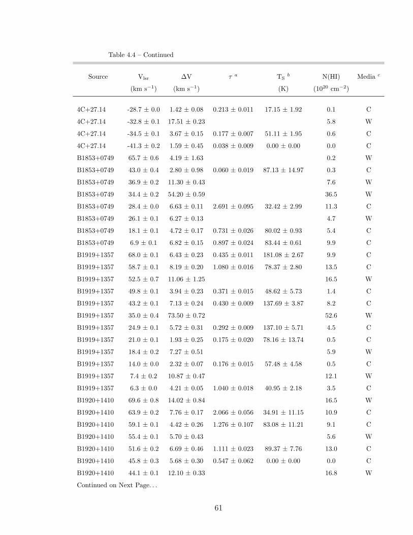
Table 4.4 – Continued

Source Vlsr ∆V τ a TSb N(HI) Media c

(km s−1) (km s−1) (K) (1020 cm−2)

4C+27.14 -28.7 ± 0.0 1.42 ± 0.08 0.213 ± 0.011 17.15 ± 1.92 0.1 C

4C+27.14 -32.8 ± 0.1 17.51 ± 0.23 5.8 W

4C+27.14 -34.5 ± 0.1 3.67 ± 0.15 0.177 ± 0.007 51.11 ± 1.95 0.6 C

4C+27.14 -41.3 ± 0.2 1.59 ± 0.45 0.038 ± 0.009 0.00 ± 0.00 0.0 C

B1853+0749 65.7 ± 0.6 4.19 ± 1.63 0.2 W

B1853+0749 43.0 ± 0.4 2.80 ± 0.98 0.060 ± 0.019 87.13 ± 14.97 0.3 C

B1853+0749 36.9 ± 0.2 11.30 ± 0.43 7.6 W

B1853+0749 34.4 ± 0.2 54.20 ± 0.59 36.5 W

B1853+0749 28.4 ± 0.0 6.63 ± 0.11 2.691 ± 0.095 32.42 ± 2.99 11.3 C

B1853+0749 26.1 ± 0.1 6.27 ± 0.13 4.7 W

B1853+0749 18.1 ± 0.1 4.72 ± 0.17 0.731 ± 0.026 80.02 ± 0.93 5.4 C

B1853+0749 6.9 ± 0.1 6.82 ± 0.15 0.897 ± 0.024 83.44 ± 0.61 9.9 C

B1919+1357 68.0 ± 0.1 6.43 ± 0.23 0.435 ± 0.011 181.08 ± 2.67 9.9 C

B1919+1357 58.7 ± 0.1 8.19 ± 0.20 1.080 ± 0.016 78.37 ± 2.80 13.5 C

B1919+1357 52.5 ± 0.7 11.06 ± 1.25 16.5 W

B1919+1357 49.8 ± 0.1 3.94 ± 0.23 0.371 ± 0.015 48.62 ± 5.73 1.4 C

B1919+1357 43.2 ± 0.1 7.13 ± 0.24 0.430 ± 0.009 137.69 ± 3.87 8.2 C

B1919+1357 35.0 ± 0.4 73.50 ± 0.72 52.6 W

B1919+1357 24.9 ± 0.1 5.72 ± 0.31 0.292 ± 0.009 137.10 ± 5.71 4.5 C

B1919+1357 21.0 ± 0.1 1.93 ± 0.25 0.175 ± 0.020 78.16 ± 13.74 0.5 C

B1919+1357 18.4 ± 0.2 7.27 ± 0.51 5.9 W

B1919+1357 14.0 ± 0.0 2.32 ± 0.07 0.176 ± 0.015 57.48 ± 4.58 0.5 C

B1919+1357 7.4 ± 0.2 10.87 ± 0.47 12.1 W

B1919+1357 6.3 ± 0.0 4.21 ± 0.05 1.040 ± 0.018 40.95 ± 2.18 3.5 C

B1920+1410 69.6 ± 0.8 14.02 ± 0.84 16.5 W

B1920+1410 63.9 ± 0.2 7.76 ± 0.17 2.066 ± 0.056 34.91 ± 11.15 10.9 C

B1920+1410 59.1 ± 0.1 4.42 ± 0.26 1.276 ± 0.107 83.08 ± 11.21 9.1 C

B1920+1410 55.4 ± 0.1 5.70 ± 0.43 5.6 W

B1920+1410 51.6 ± 0.2 6.69 ± 0.46 1.111 ± 0.023 89.37 ± 7.76 13.0 C

B1920+1410 45.8 ± 0.3 5.68 ± 0.30 0.547 ± 0.062 0.00 ± 0.00 0.0 C

B1920+1410 44.1 ± 0.1 12.10 ± 0.33 16.8 W

Continued on Next Page. . .

61

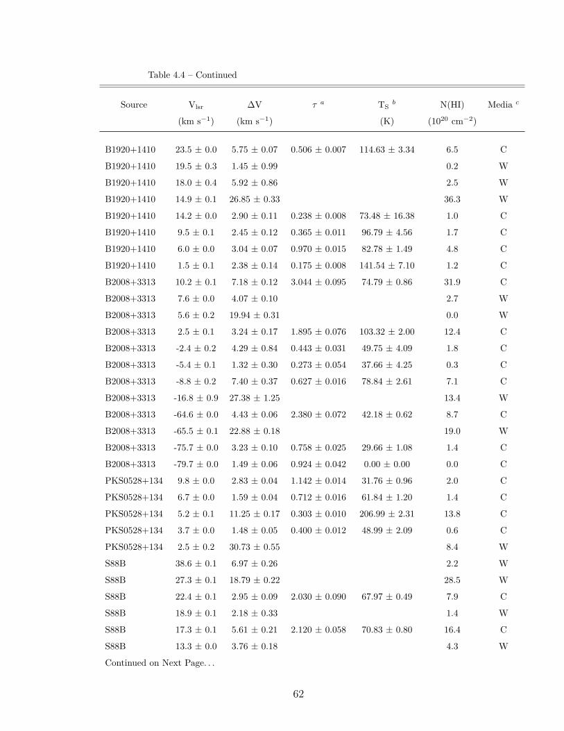
Table 4.4 – Continued

Source Vlsr ∆V τ a TSb N(HI) Media c

(km s−1) (km s−1) (K) (1020 cm−2)

B1920+1410 23.5 ± 0.0 5.75 ± 0.07 0.506 ± 0.007 114.63 ± 3.34 6.5 C

B1920+1410 19.5 ± 0.3 1.45 ± 0.99 0.2 W

B1920+1410 18.0 ± 0.4 5.92 ± 0.86 2.5 W

B1920+1410 14.9 ± 0.1 26.85 ± 0.33 36.3 W

B1920+1410 14.2 ± 0.0 2.90 ± 0.11 0.238 ± 0.008 73.48 ± 16.38 1.0 C

B1920+1410 9.5 ± 0.1 2.45 ± 0.12 0.365 ± 0.011 96.79 ± 4.56 1.7 C

B1920+1410 6.0 ± 0.0 3.04 ± 0.07 0.970 ± 0.015 82.78 ± 1.49 4.8 C

B1920+1410 1.5 ± 0.1 2.38 ± 0.14 0.175 ± 0.008 141.54 ± 7.10 1.2 C

B2008+3313 10.2 ± 0.1 7.18 ± 0.12 3.044 ± 0.095 74.79 ± 0.86 31.9 C

B2008+3313 7.6 ± 0.0 4.07 ± 0.10 2.7 W

B2008+3313 5.6 ± 0.2 19.94 ± 0.31 0.0 W

B2008+3313 2.5 ± 0.1 3.24 ± 0.17 1.895 ± 0.076 103.32 ± 2.00 12.4 C

B2008+3313 -2.4 ± 0.2 4.29 ± 0.84 0.443 ± 0.031 49.75 ± 4.09 1.8 C

B2008+3313 -5.4 ± 0.1 1.32 ± 0.30 0.273 ± 0.054 37.66 ± 4.25 0.3 C

B2008+3313 -8.8 ± 0.2 7.40 ± 0.37 0.627 ± 0.016 78.84 ± 2.61 7.1 C

B2008+3313 -16.8 ± 0.9 27.38 ± 1.25 13.4 W

B2008+3313 -64.6 ± 0.0 4.43 ± 0.06 2.380 ± 0.072 42.18 ± 0.62 8.7 C

B2008+3313 -65.5 ± 0.1 22.88 ± 0.18 19.0 W

B2008+3313 -75.7 ± 0.0 3.23 ± 0.10 0.758 ± 0.025 29.66 ± 1.08 1.4 C

B2008+3313 -79.7 ± 0.0 1.49 ± 0.06 0.924 ± 0.042 0.00 ± 0.00 0.0 C

PKS0528+134 9.8 ± 0.0 2.83 ± 0.04 1.142 ± 0.014 31.76 ± 0.96 2.0 C

PKS0528+134 6.7 ± 0.0 1.59 ± 0.04 0.712 ± 0.016 61.84 ± 1.20 1.4 C

PKS0528+134 5.2 ± 0.1 11.25 ± 0.17 0.303 ± 0.010 206.99 ± 2.31 13.8 C

PKS0528+134 3.7 ± 0.0 1.48 ± 0.05 0.400 ± 0.012 48.99 ± 2.09 0.6 C

PKS0528+134 2.5 ± 0.2 30.73 ± 0.55 8.4 W

S88B 38.6 ± 0.1 6.97 ± 0.26 2.2 W

S88B 27.3 ± 0.1 18.79 ± 0.22 28.5 W

S88B 22.4 ± 0.1 2.95 ± 0.09 2.030 ± 0.090 67.97 ± 0.49 7.9 C

S88B 18.9 ± 0.1 2.18 ± 0.33 1.4 W

S88B 17.3 ± 0.1 5.61 ± 0.21 2.120 ± 0.058 70.83 ± 0.80 16.4 C

S88B 13.3 ± 0.0 3.76 ± 0.18 4.3 W

Continued on Next Page. . .

62

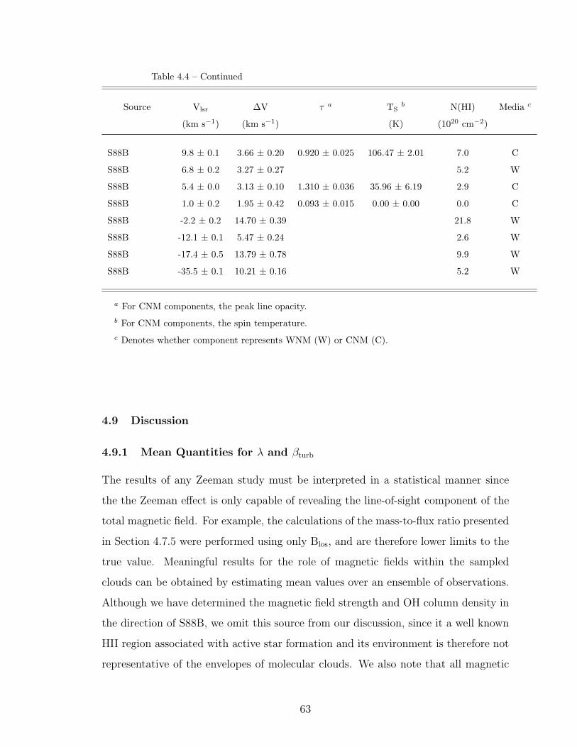
Table 4.4 – Continued

Source Vlsr ∆V τ a TSb N(HI) Media c

(km s−1) (km s−1) (K) (1020 cm−2)

S88B 9.8 ± 0.1 3.66 ± 0.20 0.920 ± 0.025 106.47 ± 2.01 7.0 C

S88B 6.8 ± 0.2 3.27 ± 0.27 5.2 W

S88B 5.4 ± 0.0 3.13 ± 0.10 1.310 ± 0.036 35.96 ± 6.19 2.9 C

S88B 1.0 ± 0.2 1.95 ± 0.42 0.093 ± 0.015 0.00 ± 0.00 0.0 C

S88B -2.2 ± 0.2 14.70 ± 0.39 21.8 W

S88B -12.1 ± 0.1 5.47 ± 0.24 2.6 W

S88B -17.4 ± 0.5 13.79 ± 0.78 9.9 W

S88B -35.5 ± 0.1 10.21 ± 0.16 5.2 W

a For CNM components, the peak line opacity.b For CNM components, the spin temperature.c Denotes whether component represents WNM (W) or CNM (C).

4.9 Discussion

4.9.1 Mean Quantities for λ and βturb

The results of any Zeeman study must be interpreted in a statistical manner since

the the Zeeman effect is only capable of revealing the line-of-sight component of the

total magnetic field. For example, the calculations of the mass-to-flux ratio presented

in Section 4.7.5 were performed using only Blos, and are therefore lower limits to the

true value. Meaningful results for the role of magnetic fields within the sampled

clouds can be obtained by estimating mean values over an ensemble of observations.

Although we have determined the magnetic field strength and OH column density in

the direction of S88B, we omit this source from our discussion, since it a well known

HII region associated with active star formation and its environment is therefore not

representative of the envelopes of molecular clouds. We also note that all magnetic

63

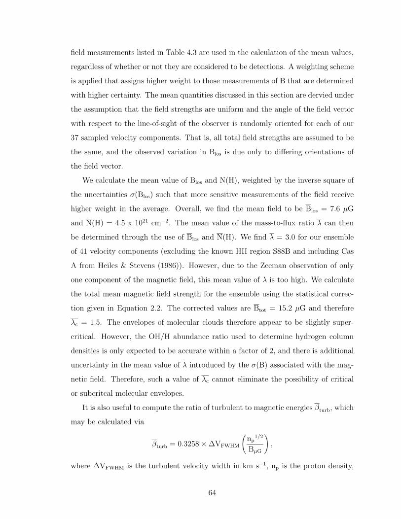
field measurements listed in Table 4.3 are used in the calculation of the mean values,

regardless of whether or not they are considered to be detections. A weighting scheme

is applied that assigns higher weight to those measurements of B that are determined

with higher certainty. The mean quantities discussed in this section are dervied under

the assumption that the field strengths are uniform and the angle of the field vector

with respect to the line-of-sight of the observer is randomly oriented for each of our

37 sampled velocity components. That is, all total field strengths are assumed to be

the same, and the observed variation in Blos is due only to differing orientations of

the field vector.

We calculate the mean value of Blos and N(H), weighted by the inverse square of

the uncertainties σ(Blos) such that more sensitive measurements of the field receive

higher weight in the average. Overall, we find the mean field to be Blos = 7.6 µG

and N(H) = 4.5 x 1021 cm−2. The mean value of the mass-to-flux ratio λ can then

be determined through the use of Blos and N(H). We find λ = 3.0 for our ensemble

of 41 velocity components (excluding the known HII region S88B and including Cas

A from Heiles & Stevens (1986)). However, due to the Zeeman observation of only

one component of the magnetic field, this mean value of λ is too high. We calculate

the total mean magnetic field strength for the ensemble using the statistical correc-

tion given in Equation 2.2. The corrected values are Btot = 15.2 µG and therefore

λc = 1.5. The envelopes of molecular clouds therefore appear to be slightly super-

critical. However, the OH/H abundance ratio used to determine hydrogen column

densities is only expected to be accurate within a factor of 2, and there is additional

uncertainty in the mean value of λ introduced by the σ(B) associated with the mag-

netic field. Therefore, such a value of λc cannot eliminate the possibility of critical

or subcritcal molecular envelopes.

It is also useful to compute the ratio of turbulent to magnetic energies βturb, which

may be calculated via

βturb = 0.3258×∆VFWHM

(np

1/2

BµG

),

where ∆VFWHM is the turbulent velocity width in km s−1, np is the proton density,

64

and B is the total magnetic field strength in µG. Assuming a typical proton density

of 100 cm−2, we find βturb = 0.08. It is clear that the magnetic energy dominates the

turbulent energies within our sample. Therefore, we find that gravitational energy

is slightly dominate over magnetic energy, and kinetic energy is smaller than either.

This differs from the model of McKee et al. (1993), which suggests that magnetic

and turbulent energies are in equilibrium, contributing approximately equally to the

support of a cloud. However, the same model predicts that clouds are approximately

2 times critical, which is nearly in agreement with our calculated λc = 1.5.

It is interesting to consider separately the results of λ and βturb in the direction of

the Galactic center (R.A. ≈ 3h - 7h) and the Galactic anti-center (R.A. ≈ 19h - 21h).

For the lines-of-sight in the direction of the Galactic center, we find Btot = 15.2 µG,

N(H) = 8.3 x 1021 cm−2, and λc = 2.8. In the direction of the Galactic anti-center, we

find Btot = 15.2 µG, N(H) = 3.2 x 1021 cm−2, and λc = 1.1. Therefore, the magnetic

field appears to be constant throughout the two regions, but lines-of-sight toward the

Galactic center region tend to have higher column densities, and thus mass-to-flux

ratios that are closer to the critical value. The value of βturb = 0.08 for both regions.

4.9.2 Visual Extinction

Mean visual extinctions can be calculated from the mean value of the total hydrogen

column density through Equation 2.11. We find AV = 2.4 magnitudes for the sample,

while the subsets of components in the direction of the Galactic center and anti-center

yield slightly higher and lower values of 4.4 and 1.7, respectively. The observed AV

is approximately 3 times less than the 8 magnitudes typically quoted as the mean

extinction for lines-of-sight through GMCs. This suggests that our lines-of-sight may

not sample environments characteristic of GMCs. One possibility is that our lines-of-

sight preferentially sample lower column densities through GMCs than average. For

example, we may be looking through the outer edge of a self-gravitating GMC such

that the path length and column density are lower than the average value. It is also

possible that we are sampling diffuse clouds that are not gravitationally bound but

have higher column densities than the average diffuse cloud. The interpretation of

65

our results depends critically on which of these scenarios is correct. If we are truly

probing GMCs, then our mean mass-to-flux ratio and the observation of subcritical

gas along individual site lines suggest that clouds as a whole begin approximatly

critical and evolve into a supercritical state. This is the progression proposed by the

magnetically driven star formation theory. On the other hand, if the lines-of-sight

sample diffuse clouds, then the detection of subcritical gas is not surprising, since

these clouds are not gravitationally bound.

The line-of-sight components for which subcritical gas is observed all appear to

lie near the lower end of the column density range sampled by OH in Figure 4.5. In

addition, the trend of the ensemble of new results is generally well-matched to that

of HI Zeeman measurements of diffuse clouds from the Millennium Survey. This may

support the possibility that the sample consists of clouds that are more diffuse in

nature than GMCs.

A more quantitiative way to determine the nature of the sampled lines-of-sight is

to consider the mean value of βturb. The HI diffuse clouds observed as part of the

Millennium Survey were found to have values of βturb ≈ 1.3. The calculated value of

0.08 discussed in Section 4.9.1 for the current study is much lower, indicating that the

objects observed in OH are not similar to the mean HI diffuse clouds. This suggests

that the sampled lines-of-sight pass through GMC regions with lower-than-average

column densities.

4.9.3 Ratio of Molecular to Atomic Gas

Observation of both OH and HI absorption lines along many lines-of-sight provides

new information about the relative abundance of atomic and molecular gas in GMCs.

This relative abundance is not currently well-determined.

Crutcher (1979) give the OH to total hydrogen abundance ratio as:

N(OH)

N(H)= 4 × 10−8,

where N(H) = N(HI) + 2N(H2). Comparison of OH and HI column densities for

line components of similar velocity yields a mean OH-HI abundance of 9.3 x 10−7, a

66

value nearly 20 times larger than the OH-H ratio, suggesting that molecular hydrogen

dominates our lines-of-sight. The absorption profiles used in this calculation often

consisted of several blended velocity components, especially in the direction of low-

latitude target sources. In such cases, the OH-HI ratio was computed using the

sum of the column densities for all confused components, possibly leading to large

uncertainties in the ratio. Combining this calculated OH-HI abundance ratio with

the OH-H ratio from Crutcher (1979), we find the mean ratio of molecular to atomic

hydrogen along our sight lines to be N(H2)/N(HI) = 7.9.

4.9.4 Future Work

As briefly discussed in Section 4.9.2, the interpretation of our mass-to-flux ratio results

depends critically upon the details of the sampled lines-of-sight. For example, we

found the mean extinction for our sight lines to be a factor of three less than the

“typical” extinction expected for GMCs. Is this low value the result of observations of

diffuse clouds, or are we preferentally sampling lower density regions of self-gravitating

GMCs? If diffuse, then our individual subcritical gas detections are not surprising,

but results are significant if they reflect conditions in GMCs as a whole. Does any

individual line-of-sight pass through higher density molecular cloud cores? If so, then

the mass-to-flux ratio results are not representative of the general regions of molecular

clouds and should be excluded from the statistical interpretation. To answer these

questions, we have used the VLA and CARMA (Combined Array for Research in

Millimeter-wave Astronomy) to obtain information in the direction of a subset of our

target sources. The analysis of this data, and possible future observations of more

sight lines, will help to identify the nature of the sampled gas.

In addition to the OH main line and HI data discussed in this dissertation, we also

possess 1612 and 1720 MHz OH absorption line data in the direction of each target

source. These satellite lines exhibit the anamolous Zeeman effect, as opposed to the

normal Zeeman effect of the main lines and HI. We plan to apply the spectral synthesis

code Cloudy to reproduce all four observed OH transitions for each sight line using

a set of input interstellar conditions. The simulations would yield values of column

67

density and excitation temperatures for all four lines, allowing for investigation of

how closely matched the simulated column densities and excitation temperatures are

with the observed values for the main line transitions. In addition, the simulations

would yield values of volume density for each line-of-sight, a parameter that cannot

be directly calculated from our current observations. Further insight to the role

of the magnetic field could be found through comparison of the simulated volume

density to the observed field strength in the direction of each target source. The two

prevailing theories of star formation predict that the magnetic field strength scales

as |B| ∝ nκ, where n is the volume density and κ is a constant equal to 23

or 12

for

the turbulence-driven and magnetically-driven theories, respectively (Crutcher et al.,

2010, and references therein).

Existing HI observations can yield independent calculations of the mass-to-flux

ratio. As discussed in Section 4.8, HI observations are subject to many instrumental

effects that must be accounted for to accurately derive magnetic field strengths. We

plan to conduct a complete analysis of these effects and infer field strengths and mass-

to-flux ratios from the data. Comparison of the HI results for velocity components

that also appear in the OH absorption profiles to the OH results will be of particular

interest since the absorption originates from the same cloud along the line-of-sight.

Since the Zeeman effect only reveals the line-of-sight magnetic field strength, the

results of the survey as a whole must be taken statistically. Therefore, a large sam-

ple is necessary to ensure that small observed values of Blos do not reflect larger

field strengths that lie nearly in the plane of the sky. The observations of the cur-

rent Arecibo absorption survey was limited by the need to observe bright continuum

sources that lie behind the molecular gas of interest to achive absorption profiles. A

much larger statistical sample may be obtained by searching for the Zeeman effect in

OH emission lines using the NRAO Green Bank Telescope (GBT). Such an emission

line survey has the potential to yield several additional measurements of the mass-

to-flux ratio since the production of emission lines does not require the presence of

a backgrund continuum source. However, a large amount of integration time would

be required since OH emission lines are weaker than their absorption counterparts

68

and are therefore less sensitive to the Zeeman effect. The results from the current

Arecibo absorption survey may be complimented by a GBT proposal for an emission

line survey in the near future.

4.10 Summary and Conclusions

We have conducted the first observational survey aimed at determining the role of

magnetic fields in molecular clouds as a whole. The crucial parameter for quantifying

the significance of the molecular cloud support provided by magnetic fields is the

mass-to-flux ratio λ, a measure of the ratio of gravitational energy to magnetic energy

within a cloud. Previous studies have determined the mass-to-flux ratio in both

diffuse HI clouds and in the cores of GMCs. The results of these studies indicate

the diffuse clouds are magnetically dominated (subcritical), while cloud cores are

slightly gravitationally dominated (supercritical). However, if we are to understand

the evolution of GMCs as a whole, the mass-to-flux ratio in the intercore envelopes

of the clouds must also be determined.

To determine the mass-to-flux ratio in molecular clouds, we have conducted Zee-

man observations of the four 18 cm OH ground state transitions with the Arecibo

telescope. We sample the line-of-sight toward 22 extragalactic continuum sources

that lie behind Galactic molecular clouds. Observations yielded 37 independent cal-

culations of the mass-to-flux ratio in the envelopes of molecular clouds. The Zeeman

effect is detected in 5 velocity components along the line-of-sight. However, the cal-

culation of the mass-to-flux ratio does not require magnetic field detections, only

sensitive measurements of the field.

Calculation of the mass-to-flux ratio for individual velocity components yields

the first evidence for magnetically subcritical molecular gas. The majority of the

subcritical measurements stem from among the most sensitive Zeeman measurements

in our sample, with some of them above the 3σ detection threshold. We therefore

believe these measurements to be significant and accurate characterizations of the

absorbing gas. However, the line-of-sight magnetic field strengths determined via

the Zeeman effect are lower limits to the total field strength. Therefore, meaningful

69

results of the survey as a whole must be obtained by considering the mean results of

a large ensemble of observations.

We calculate mean value of the mass-to-flux ratio using the average Blos and N(H)

weighted by the inverse square uncertainties of the magnetic field. We find a mean

value of λ = 3.4. However, this value is an upper limit to the mass-to-flux ratio since

the Zeeman effect yields lower limits on the field. Using a statisitical correction to

infer the total magnetic field strength from the Zeeman measurement of the line-of-

sight component, we have calculated the mean ratio corrected for the total field. The

corrected value is found to be λc = 1.5, suggesting that GMCs are critical to slightly

supercritical. However, uncertainties involved in the calculation of this value cannot

eliminate the possiblity of subcritical molecular clouds.

The average visual extinction along our lines of sight was found to be AV = 2.4 mag-

nitudes, approximately a factor of three lower than the 8 magnitudes generally ac-

cepted for the mean extinction through GMCs. This suggests that our lines-of-sight

may not sample molecular gas characteristic of GMCs. One interpretation of the low

extinction is that we are sampling self-gravitating GMCs, but our sight lines pass

through the edges of the clouds, where the column densities and hence exitinctions

are lower. A second scenario is that we are not observing GMCs at all, but rather dif-

fuse molecular material that is not gravitationally bound. The interpretation of our

results and the significance of magnetically subcritical results depends upon which

scenario is correct. Calculation of the ratio of turbulent to magnetic energies yields

βturb = 0.08, much lower than the value of 1.3 that was found for HI diffuse clouds

in the Millennium Survey. This indicates that our sampled lines-of-sight are much

different from the diffuse clouds sampled in HI. Therefore, it is likely that we are pref-

erentially sampling column densities of GMCs that are much lower than the mean

value.

There are currently two competing theories of star formation that assign different

roles to the magnetic field. In the magnetically driven theory of star formation,

the magnetic field plays a leading role, providing sufficient support for clouds to

begin their lifetimes as subcritical bodies. This theory predicts that λ should be

70

approximately critical to slightly subcritical. The turbulence driven theory of star

formation predicts that magnetic fields are too weak to be physically important in the

star formation process and hence λ is predicted to be supercritical, perhaps as large as

100. Can the results of our study distinguish between these two theories? Assuming

that we are truly sampling GMCs, we find a value of λ that is approximately critical

to slightly supercritical and is therefore consistant with both theories. However, the

measurements of subcritical gas in individual velocity components along our lines-

of-sight are believed to be significant. These measurements support only one model:

the magnetically driven theory of star formation. The turbulence model does not

allow for subcritical molecular gas. Therefore, our results appear to be in general

agreement with the concept of magnetically supported clouds with column densities

a factor of 3 less than “standard” GMCs.

Copyright c© Kristen Lynn Thompson, 2012.

71

Chapter 5

Jansky VLA Observations Toward the Sagittarius A Complex

5.1 Introduction

At a distance of approximately 8 kpc (e.g., Eisenhauer et al., 2003; Gillessen et

al., 2009; Reid, 1993), the center of our Galaxy is a very complex and dynamic

region called the Sagittarius (Sgr) A complex, which plays host to a wide array of

astrophysical processes. The Galactic center lies in the direction of the Sagittarius

constellation, but is hidden from our view by a vast number of dense molecular clouds

which are opaque to the visible regime of the electromagnetic spectrum. Hence,

much of what we know about this region comes from radio or infrared wavelength

observations.

At the heart of the Galactic center is Sgr A*, a compact radio source. Sgr A* is

coincident with the rotational center of the Galaxy and is the location of a quiescent

supermassive black hole harboring over 4 x 106 solar masses (Gillessen et al., 2009).

The thermal HII region Sgr A West appears as a three armed spiral in the plane of the

sky and is composed of the Northern Arm, the Eastern Arm, the Western Arc, and

the Bar that connects the three arm components. The Northern Arm and Eastern

Arm are thought to be ionized streamers of material falling in toward Sgr A* (e.g., Lo

& Claussen, 1983; Ekers et al., 1983). It is generally accepted that the “minispiral”

of Sgr A West is centered on Sgr A*. Surrounding Sgr A West, with an inner radius

of approximately 1.5 pc, is the circumnuclear disk (CND), an asymmetric torus-like

structure of gas and dust. The CND has been traced in HCN by Gusten et al. (1987)

and appears as a nearly complete ring rotating about Sgr A*. Encompassing these

structures is a large non-thermal source, Sgr A East. The large (r ≈ 10 pc) shell-

like structure is thought to be a Galactic supernova remnant (SNR). This shell is

elongated along the Galactic plane and offset from Sgr A* by approximately 2.1 pc

to the northeast, such that the western edge of Sgr A East blends with the Western

72

Arc of Sgr A West. To the east of Sgr A East lies the well-known giant molecular

cloud M-0.02-0.07, sometimes called the 50 km s−1 cloud. The cloud is thought to be

interacting with the northeastern edge of the expanding Sgr A East, triggering star

formation and resulting in the flattened outer side of the SNR in this direction and

the production of a chain of 4 compact HII regions (Yusef-Zadeh et al., 1996). These

features are evident in the 18-cm continuum map shown in Figure 5.1.

5.2 Previous Studies

There have been a handful of previous Zeeman studies aimed at detecting the line-

of-sight magnetic field in the Galactic center region via the Zeeman effect in radio

frequency spectral lines. Killeen, Lo, & Crutcher (1992), hereafter KLC, used the

BnA configuration of the VLA to observe 1667 MHz OH in absorption against the

Sgr A complex. Magnetic field strengths were determined in three regions with OH

absorption features identifiable with the CND: the “redshifted cloud” to the west of

Sgr A West identified with HCN by Gusten et al. (1987), and material to the north

and south of Sgr A West that corresponds to the northern and southern portions

of the CND. With only 7 hours of on-source integration time, the sensitivity of the

data is marginal, and as a result, the Zeeman effect was not able to be detected

in any individual synthesized beam. The authors therefore implement two fitting

techniques that increase the signal-to-noise ratio to allow detection of weak magnetic

fields; spatial averaging and spatial summing. Spatial averaging is the technique

of averaging together all spectra from within a given spatial region, significantly

lowering the noise in the resulting spectrum. However, it is important to note that if

the spectral shapes from within the region are not all the same, the signal, as well as

the noise, can be averaged down. In the case of spatial summing, all of the spectra

from within a given spatial region are placed head-to-tail, and are fit simultaneously

as one long spectrum by the algorithm. For both techniques the Zeeman splitting, and

therefore the magnetic field vector, is assumed to be constant within the region. It

is expected that spatial summing produces slightly better signal-to-noise ratios than

does spatial averaging. The authors performed spatial averaging and spatial summing

73

over several isolated regions within the three larger features of the CND mentioned

above. Spatial averaging yielded no Zeeman detections over any of the three features

at a 3σ confidence level. Spatial summing led to a 7σ Zeeman detection in one

isolated area of the southern region of the CND and a few marginal 4σ detections

in the southern and northern regions. The magnitude of the line-of-sight magnetic

field was found to be of order -2 mG (by convention, negative values indicate field

directions toward the observer). The authors carried out the same analysis in a few

other regions in the central 200 pc of the Galactic center not associated with the

CND, resulting in three sigma upper limits of 1-2 mG. However, this study has a

severe limitation: the velocity coverage of this study was not sufficient to sample the

full range of absorbing OH gas toward the Galactic center (e.g., Zhao, Goss, & Ho,

1995). In addition, since spatial summing and spatial averaging assume the field is

constant over some defined area, information is lost about field variations on smaller

angular scales.

Plante et al. (1995) used the VLA to search for HI Zeeman splitting toward

Sgr A West. Zeeman analysis was performed over HI absorption in the northern

region of the CND corresponding to the HCN of Gusten et al. (1987). Unlike the

study of KLC, the Zeeman effect was detected at the 3σ level on a pixel-by-pixel basis

at a few locations in the map, with field strengths |Blos| ∼ 2 - 4 mG. To improve sen-

sitivity to Blos, the authors employed spatial averaging and spatial summing. Spatial

averaging revealed Zeeman detections in 7 boxes within the northern region of the

CND. Consistent with the results of KLC, negative milligauss fields were detected.

However, one isolated region in which spatial summing was performed was chosen to

match the region of KLC. Plante et al. (1995) were unable to confirm the marginal 4σ

detection reported by the previous authors in this region. Whereas spatial summing

yielded all detections in the previous study, only spatial averaging revealed significant

Zeeman results in HI. The authors point out that the gas densities traced by HI are

different from those traced by OH in the previous study. The OH absorption is likely

due to the denser portions of the cloud, whereas HI observations probe more diffuse

gas. This could cause the Zeeman signal to be reduced below detectable levels.

74

Additional studies aimed at determining field strengths using methods other than

Zeeman splitting have been carried out. A study of dust grain alignment by Aitken

et al. (1991) suggested fields of at least 10 mG in the northern region of the CND.

Gusten et al. (1987) also report strengths of∼ 10 mG from studies of 100 µm emission.

Faraday rotation studies of the Arc source near the Galactic center yield strengths

of 10 - 100 µG (e.g., Tsuboi et al., 1986; Sofue et al., 1987). It is clear from these

studies that magnetic field strengths in the Galactic center region have not been well

determined. Current estimates of Galactic center magnetic field strengths range from

10 µG to 10 mG. Additional studies are needed with increased velocity coverage and

sensitivity in order to constrain the field in this region.

5.3 Project Goals

Previous studies have not led to conclusive results as to the strength of magnetic fields

in the Galactic center region. The integration times of KLC and Plante et al. (1995)

were relatively small. The rms noise of a telescope array is given by the radiometer

equation,

∆Im =K√

N(N− 1)(NIFTint∆νM)mJy, (5.1)

where the constant K corrects for the system temperature and antenna efficiency, N

is the number of antennas in the array, Tint is the total on-source integration time

in hours, ∆νM is the effective continuum bandwidth or spectral-line channel width

in MHz, and NIF is the number of intermediate frequency channels (from 1 to 4)

or spectral line channels which will be combined in the output image. Therefore,

the longer the integration time, the greater the signal-to-noise (S/N) ratio. It is

possible that the sensitivity of previous studies were sufficiently small that the Zeeman

splitting was “masked” by random noise. A better S/N ratio could allow the field to

be detected on a pixel-by-pixel basis, possibly revealing continuous variations in the

field strength across the CND, rather than relying on spatial summing or averaging

techniques to detect weak fields. We therefore aim to achieve increased sensitivity to

the Zeeman effect through longer on-source integration times.

75

A second shortcoming of the previous OH study conducted by KLC is that the

velocity coverage was severely limited, extending only to approximately 120 km s−1,

causing a significant portion of the extended absorbing gas to be missed. This could

lead to inaccurate fits of the magnetic field since in several cases the absorption lines

were cut off at the edge of the bandpass. Therefore, we have obtained full velocity OH

absorption spectra for the regions of the CND studied by the previous authors. The

improved sensitivity and expanded velocity coverage, combined with L-band receiver

upgrades that have taken place since the time of the previous observations, allow for

the best determination of field strengths in the central few parsecs of the Galactic

center region to date.

5.4 Observations and Data Reduction

Further observations of the Sgr A complex were made using the BnA configuration of

the VLA in October 1999 and February 2001. Right and left circular polarizations of

the 1667 MHz OH line were observed simultaneously. The spectrometer was set up

to provide 3.12 MHz total bandwidth distributed across 128 channels, resulting in a

velocity resolution of 4.4 km s−1 channel−1, doubling the velocity coverage of KLC.

Observations of 3C48 and 3C286 were performed for primary flux and passband

calibration, while 1748-253 was used for phase calibration. In order to minimize

instrumental effects that may arise from gain differences in the two IF feeds, the

sense of circular polarization was periodically toggled between bands using the front-

end transfer switch. Our on-source Sgr A integration time totaled 34.5 hours, nearly

5 times that of previous studies. Combining our longer integration time with VLA

L-band improvements, our data should have approximately 4 times the sensitivity of

previous studies. Further details of these observations can be found in Table 5.1.

Calibration, editing, deconvolution, and imaging of the visibility data was per-

formed using the Astronomical Image Processing System (AIPS) of the NRAO. To

ensure proper gain calibration, the data for each front-end transfer switch position

were calibrated separately and later combined. In addition, calibration and flagging

of bad data was performed separately for data sets obtained on different days. Un-

76

fortunately, the visibility data obtained during our February 8, 2001 observing run

was so heavily corrupted by radio-frequency interference (RFI) that is was unsal-

vageable and excluded from our final results. Portions of the remaining observations

also required extensive flagging, resulting in approximately 16% of our original data

being discarded. This lowered our initial on-source observing time from 34.5 hours to

roughly 28, as reflected in Table 5.1. Even though this reduction in observing time

negatively affected our sensitivity, our signal-to-noise ratio is still higher than those

of previous studies. Stokes I (RCP + LCP) and V (RCP - LCP) image cubes were

constructed from the calibrated visibility data. Slight natural weighting was used,

emphasizing shorter array spacings and therefore decreasing the angular resolution

but increasing the signal-to-noise ratio. The data were then deconvolved using the

CLEAN task in AIPS to remove spurious effects caused by the discrete, rather than

continuous, sampling of the u-v plane by the interferometer. Some image analysis

and spatial averaging of the image cubes was performed using the CASA (Common

Astronomy Software Application) fits reader CASA Viewer.

Additional post-calibration analysis and magnetic field derivations were carried

out using the MIRIAD (Multichannel Image Reconstruction and Image Analysis

and Display) software package of the Berkeley-Illinois-Maryland Array (BIMA). The

Stokes I and Stokes V spectra were fit simultaneously for Blos using the maximum

likelihood technique described by Sault et al. (1990). The MIRIAD task ‘zeestat’

was used to perform the fits. When spatial averaging was used, ‘zeesim’ was run

to get reliable error estimates for the field derived by ‘zeestat.’ The Zeeman effect

was unable to be detected on a pixel-by-pixel basis, so spatial summing and spatial

averaging were employed to raise the signal-to-noise in an attempt to detect weak

magnetic fields (see Section 5.2 for details about these techniques).

77

5.5 Results

5.5.1 The 18 cm Continuum

Figure 5.1 shows the VLA 18 cm OH continuum emission from Sgr A. The location

of the radio source Sgr A* is indicated by the cross and linear offsets are arcseconds

from Sgr A*. The three-armed “minispiral” of the thermal Sgr A West feature and

the non-thermal Sgr A East shell are clearly visible. To the east of Sgr A East, a

chain of four compact HII regions can be seen. These HII regions are thought to be

the result of the well-known 50 km s−1 giant molecular cloud M-0.02-0.07 interacting

with the expanding Sgr A East supernova remnant, inducing star formation at the

boundary (Yusef-Zadeh et al., 1996). Another clear feature in the continuum image

is the presence of linear structure to the southeast of Sgr A*. These same features are

evident in the 20 cm continuum maps of Plante et al. (1995) and Yusef-Zadeh et al.

(2004), although they are not as pronounced. Yusef-Zadeh et al. (2004) identify sev-

eral filamentary structures throughout the Galactic center and many features present

in their high-resolution continuum map of the Sgr A complex are also identifiable in

the 18 cm map presented here.

The relationship of the large parallel filaments to the southeast of Sgr A* in Figure

5.1 to those identified by Yusef-Zadeh et al. (2004) is not clear. They appear to be

broader and more extended than other similar structures in the region and seem to

be preferentially oriented parallel and perpendicular to one another. Although they

appear at the southern boundary of the non-thermal ring, they are angled such that

they do not follow the locus of the shell and therefore do not seem to be directly

associated with Sgr A East. We find the continuum flux at the location of Sgr A* to

be 0.64 Jy.

5.5.2 Sgr A* 18 cm Absorption Spectrum

The 1667 MHz absorption profile toward Sgr A* is shown in Figure 5.2. Several

velocity components attributed to various features of the Galactic center are clearly

visible across a 400 km s−1 absorbing range. These features are discussed below.

78

Absorption at 165 km s−1 and -135 km s−1 is attributed to clouds in the expand-

ing molecular ring (EMR). The EMR is comprised of a number of molecular clouds

orbiting around the Galactic center at a radius of ∼ 200 pc. The ring is thought to

be centered on the Galactic center and is slowly expanding. The -135 km s−1 com-

ponent is due to the approaching gas located on the near side of the EMR, while the

165 km s−1 component arises from the receding gas on the far side. Both spectral

features are readily observed in emission spectra, but only the -135 km s−1 feature has

been seen in absorption against continuum sources in the Galactic center. However,

the 165 km s−1 absorption can be clearly seen in the 1667 MHz OH absorption profile

presented here.

The 50 km s−1 component arises from the 50 km s−1 molecular cloud complex

located within 10 kpc of the Galactic center. These clouds are believed to be inter-

acting with the Sgr A East non-thermal shell, inducing star formation, and producing

the chain of 4 compact HII regions visible to the east of Sgr A East in the 18 cm

continuum image (Yusef-Zadeh et al., 1996).

The components near 0 km s−1 result from absorption by local clouds within a few

kiloparsecs of the solar neighborhood. Contribution from low velocity clouds located

near the Galactic center is also expected.

HI absorption profiles in the direction of Sgr A* show a strong absorption compo-

nent at approximately -53 km s−1. This component is also present in the OH profile,

but is much weaker. The absorption is attributed to the 3 kpc arm, a spiral arm of

the Milky Way located 3 kpc from the Galactic center.

The high negative velocity cloud at -180 km s−1 was discovered by Gusten &

Downes (1981). Subsequent studies suggested this gas was associated with the ex-

panding molecular ring with absorption at -135 km s−1 (e.g., Liszt & Burton, 1993).

Zhao, Goss, & Ho (1995) conducted high angular resolution observations of the fea-

ture in the HI and OH lines using both the A and B array configurations of the

VLA. Absorption at -180 km s−1 was prominent in both the 1665 and 1667 MHz OH

transitions and the ratio of 1667/1665 MHz optical depths was found to be ≈ 1.8,

suggesting optically thin OH lines in LTE. Both the FWHM velocity width and op-

79

tical depth of the OH lines were found to increase significantly when observed with

the larger beam of the B array. However, the same increase in opacity and line width

were not observed toward the -135 km s−1 feature, suggesting that the properties

of the -180 km s−1 and -135 km s−1 gas are much different. They suggest that the

source of the absorbing gas is a tidally disrupted high-velocity cloud flowing toward

the Galactic center.

5.5.3 The Redshifted Cloud

The redshifted cloud has been identified in the HCN survey of Gusten et al. (1987) and

lies near Sgr A West, just west of Sgr A*. The HCN survey revealed a complete molec-

ular ring of gas surrounding the Galactic center with dimensions of approximately

4.8 x 2.5 pc. The majority of this molecular gas has been found to demonstrate a

general large scale rotation pattern. However, the redshifted cloud does not appear

to participate in this rotation and appears to have a fairly constant radial velocity

of ∼ 90 km s−1. Gusten et al. (1987) argue that the cloud is associated with the inner

Galaxy, although its relationship to the CND is not clear.

Figure 5.3 shows the integrated OH absorption over velocities 35 < v < 123 km s−1

in the direction of the redshifted cloud. Zeeman splitting was not able to be detected

on a pixel-by-pixel basis, so spatial summing and averaging were used in an attempt

to lower the noise and detect weak fields. The overlay boxes on the integrated ab-

sorption indicate the regions of highest absorption identified by KLC over which the

summing and averaging techniques were applied. Toward the goal of obtaining higher

sensitivity to the magnetic field than previous studies, the boxes were chosen to match

those of KLC. Therefore, the box numbers match those used in the previous study.

Comparison of the absorption map in Figure 5.3 with Figure 2a of KLC reveals that

the two maps are consistent.

The average spectral profiles from within boxes 2 and 4 overlayed on the intensity

map are shown in Figure 5.4. Stokes I (here, I=(RR + LL)/2) is presented in the

top panels, Stokes V in the bottom. In both Stokes I intensity profiles, absorption

from the redshifted cloud can clearly be seen at v ≈ 90 km s−1. As discussed in

80

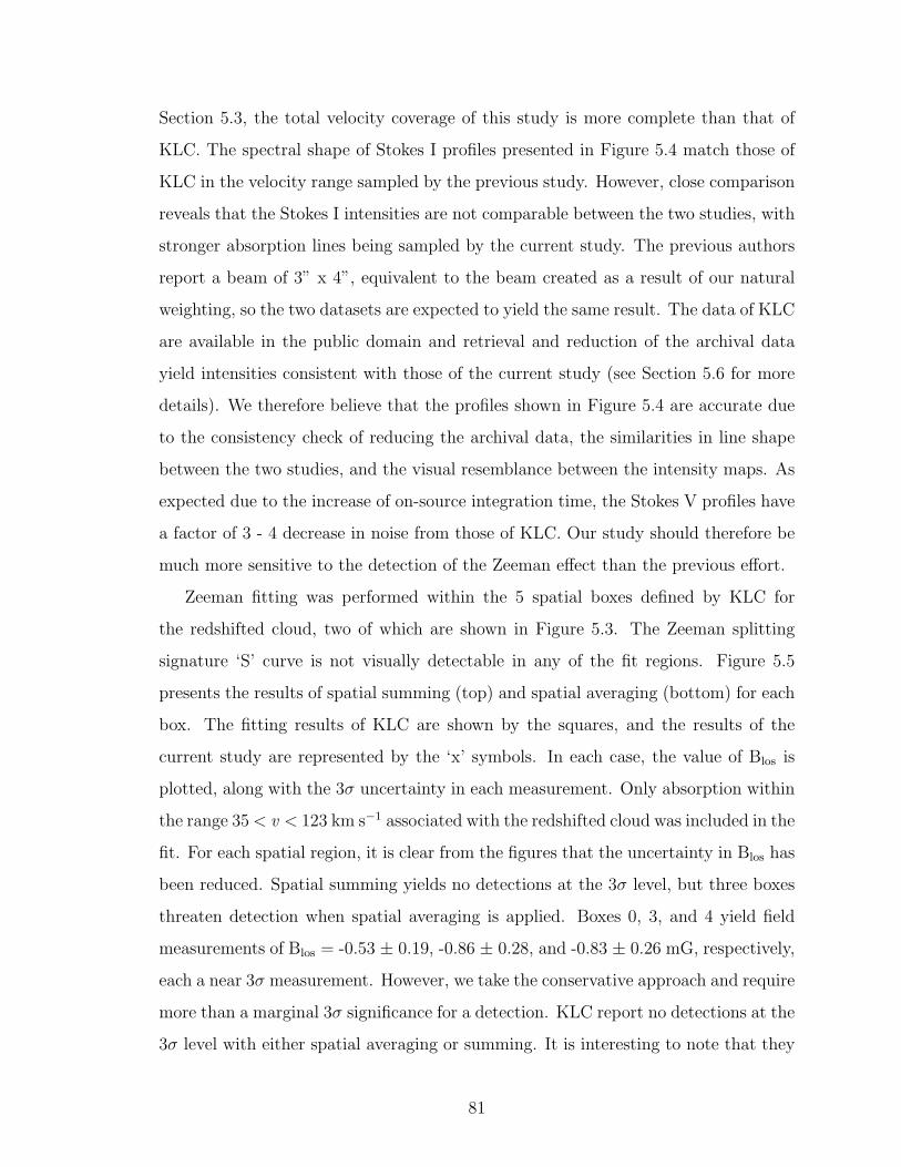
Section 5.3, the total velocity coverage of this study is more complete than that of

KLC. The spectral shape of Stokes I profiles presented in Figure 5.4 match those of

KLC in the velocity range sampled by the previous study. However, close comparison

reveals that the Stokes I intensities are not comparable between the two studies, with

stronger absorption lines being sampled by the current study. The previous authors

report a beam of 3” x 4”, equivalent to the beam created as a result of our natural

weighting, so the two datasets are expected to yield the same result. The data of KLC

are available in the public domain and retrieval and reduction of the archival data

yield intensities consistent with those of the current study (see Section 5.6 for more

details). We therefore believe that the profiles shown in Figure 5.4 are accurate due

to the consistency check of reducing the archival data, the similarities in line shape

between the two studies, and the visual resemblance between the intensity maps. As

expected due to the increase of on-source integration time, the Stokes V profiles have

a factor of 3 - 4 decrease in noise from those of KLC. Our study should therefore be

much more sensitive to the detection of the Zeeman effect than the previous effort.

Zeeman fitting was performed within the 5 spatial boxes defined by KLC for

the redshifted cloud, two of which are shown in Figure 5.3. The Zeeman splitting

signature ‘S’ curve is not visually detectable in any of the fit regions. Figure 5.5

presents the results of spatial summing (top) and spatial averaging (bottom) for each

box. The fitting results of KLC are shown by the squares, and the results of the

current study are represented by the ‘x’ symbols. In each case, the value of Blos is

plotted, along with the 3σ uncertainty in each measurement. Only absorption within

the range 35 < v < 123 km s−1 associated with the redshifted cloud was included in the

fit. For each spatial region, it is clear from the figures that the uncertainty in Blos has

been reduced. Spatial summing yields no detections at the 3σ level, but three boxes

threaten detection when spatial averaging is applied. Boxes 0, 3, and 4 yield field

measurements of Blos = -0.53 ± 0.19, -0.86 ± 0.28, and -0.83 ± 0.26 mG, respectively,

each a near 3σ measurement. However, we take the conservative approach and require

more than a marginal 3σ significance for a detection. KLC report no detections at the

3σ level with either spatial averaging or summing. It is interesting to note that they

81

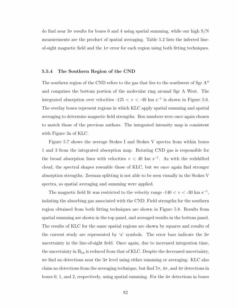
do find near 3σ results for boxes 0 and 4 using spatial summing, while our high S/N

measurements are the product of spatial averaging. Table 5.2 lists the inferred line-

of-sight magnetic field and the 1σ error for each region using both fitting techniques.

5.5.4 The Southern Region of the CND

The southern region of the CND refers to the gas that lies to the southwest of Sgr A*

and comprises the bottom portion of the molecular ring around Sgr A West. The

integrated absorption over velocities -125 < v < -40 km s−1 is shown in Figure 5.6.

The overlay boxes represent regions in which KLC apply spatial summing and spatial

averaging to determine magnetic field strengths. Box numbers were once again chosen

to match those of the previous authors. The integrated intensity map is consistent

with Figure 3a of KLC.

Figure 5.7 shows the average Stokes I and Stokes V spectra from within boxes

1 and 3 from the integrated absorption map. Rotating CND gas is responsible for

the broad absorption lines with velocities v < 40 km s−1. As with the redshifted

cloud, the spectral shapes resemble those of KLC, but we once again find stronger

absorption strengths. Zeeman splitting is not able to be seen visually in the Stokes V

spectra, so spatial averaging and summing were applied.

The magnetic field fit was restricted to the velocity range -140 < v < -30 km s−1,

isolating the absorbing gas associated with the CND. Field strengths for the southern

region obtained from both fitting techniques are shown in Figure 5.8. Results from

spatial summing are shown in the top panel, and averaged results in the bottom panel.

The results of KLC for the same spatial regions are shown by squares and results of

the current study are represented by ‘x’ symbols. The error bars indicate the 3σ

uncertainty in the line-of-sight field. Once again, due to increased integration time,

the uncertainty in Blos is reduced from that of KLC. Despite the decreased uncertainty,

we find no detections near the 3σ level using either summing or averaging. KLC also

claim no detections from the averaging technique, but find 7σ, 4σ, and 4σ detections in

boxes 0, 1, and 2, respectively, using spatial summing. For the 4σ detections in boxes

82

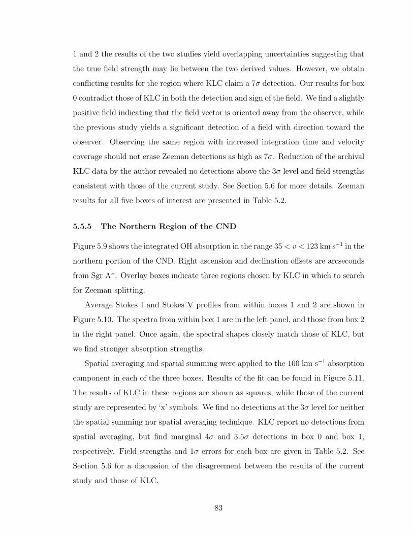
1 and 2 the results of the two studies yield overlapping uncertainties suggesting that

the true field strength may lie between the two derived values. However, we obtain

conflicting results for the region where KLC claim a 7σ detection. Our results for box

0 contradict those of KLC in both the detection and sign of the field. We find a slightly

positive field indicating that the field vector is oriented away from the observer, while

the previous study yields a significant detection of a field with direction toward the

observer. Observing the same region with increased integration time and velocity

coverage should not erase Zeeman detections as high as 7σ. Reduction of the archival

KLC data by the author revealed no detections above the 3σ level and field strengths

consistent with those of the current study. See Section 5.6 for more details. Zeeman

results for all five boxes of interest are presented in Table 5.2.

5.5.5 The Northern Region of the CND

Figure 5.9 shows the integrated OH absorption in the range 35 < v < 123 km s−1 in the

northern portion of the CND. Right ascension and declination offsets are arcseconds

from Sgr A*. Overlay boxes indicate three regions chosen by KLC in which to search

for Zeeman splitting.

Average Stokes I and Stokes V profiles from within boxes 1 and 2 are shown in

Figure 5.10. The spectra from within box 1 are in the left panel, and those from box 2

in the right panel. Once again, the spectral shapes closely match those of KLC, but

we find stronger absorption strengths.

Spatial averaging and spatial summing were applied to the 100 km s−1 absorption

component in each of the three boxes. Results of the fit can be found in Figure 5.11.

The results of KLC in these regions are shown as squares, while those of the current

study are represented by ‘x’ symbols. We find no detections at the 3σ level for neither

the spatial summing nor spatial averaging technique. KLC report no detections from

spatial averaging, but find marginal 4σ and 3.5σ detections in box 0 and box 1,

respectively. Field strengths and 1σ errors for each box are given in Table 5.2. See

Section 5.6 for a discussion of the disagreement between the results of the current

study and those of KLC.

83

5.5.6 Masers

Four 1667 MHz OH maser sources are visible in the Stokes I image cubes. Properties

of these circumstellar masers are given in Table 5.3. Identified velocities are the

approximate center velocity of the system for multiple maser components. Three

of the masers were seen by KLC, while the fourth was outside the view of their

256” x 256” image cubes. These four sources were detected by Karlsson et al. (2003)

and were also identified in 1612 MHz line by Lindqvist et al. (1992). Two of these

1667 MHz masers correspond to the strongest identified 1612 MHz lines and are also

seen in observations of 1665 MHz OH.

5.6 Discussion

The data of KLC are available in the public domain on the VLA archive site. To

address the disagreement between the results of KLC and those of the current study,

we have retrieved, calibrated, imaged, and performed our analysis on their raw data.

All calibration, editing, imaging, and deconvolution were performed using AIPS. In

an attempt to reproduce their results, the calibration of visibility data followed closely

to that outlined by KLC. However, we did not see the need for the self-calibration

executed by the previous authors, so basic calibration was performed. Stokes I and

Stokes V images were produced to have the same properties of KLC: 256 x 256 pixels,

with a pixel size of 1”, and resolution of 3” x 4”. Following imaging, several beam

artifacts were present, so the AIPS task CLEAN was used for deconvolution of the

Stokes I image cube. KLC did not perform image deconvolution, as they judged that

it was unnecessary and even undesirable.

One discrepancy between the published results of KLC and the results of the

current study is the absorption line strengths in the average Stokes I profile from

within individual regions. We find line strengths that are consistently ∼ 1.7× those

shown by KLC. In the reduction of their data, we find absorption peaks in the spatially

averaged data that have approximately the same strength as found in the more recent

study. Line strengths within the Stokes I image cubes for both reductions also agree

84

on a pixel-by-pixel basis. Therefore, the Stokes I spectral profiles are in agreement

for both our reduction of the new data and that of KLC, but disagree with the

published profiles of the previous authors. Figure 5.12 illustrates the difference in

Stokes I absorption strengths between the three data reductions from within box 3 of

the southern region of the CND. The top panel is taken from KLC, the middle panel

shows the spectrum obtained as a result of reduction of the KLC data by Thompson,

and the result of the current study is shown in the bottom panel. To be confident

that our flux scales are correct, we compared the bootstrapped flux for the phase and

bandpass calibrators obtained in the calibration process by the AIPS task GETJY to

those in the VLA calibrator manual. It was found that the fluxes are well-matched,

so we expect that our scaling is accurate.

A similar comparison was done between the maser fluxes reported by KLC and

those in the new reduction of the KLC data. KLC maser strengths were estimated

by eye from Figure 8a of their publication. Our reduction of the data reveal maser

strengths that are, on average, 1.7× those shown by KLC. Note that this ratio is

the same as that observed for the absorption line strengths. Interstellar masers are

known to be time variable, so direct comparison of the maser strengths of KLC and

those of the current study is not a useful measure of consistency between projects.

However, the spectral profile shapes and center velocities of the masers are found to

be similar between the two studies.

The ability to detect Zeeman splitting depends critically on the noise in the

Stokes V spectrum. As shown in Equation 5.1, the expected rms noise in the Stokes V

profile is proportional to (Tint×∆νM)−1/2, where Tint is the on-source integration time

and ∆νM is the channel frequency width. The more recent data has 4 times the chan-

nel width and approximately 3.5 times the on-source integration time of KLC. The

data of KLC are therefore expected to have approximately 3.7 times the rms noise

in Stokes V. Comparison of the noise within the newly reduced data of KLC and

the new observations presented in this dissertation yields the expected ratio, both in

spatial box averages and on a pixel-by-pixel basis within the Stokes V image cube.

Magnetic field strengths derived in the current study are inconsistent with those

85

reported by KLC. Magnetic field fitting was performed on the KLC data in the same

manner described in Section 5.4 for the more recent observations. Spatial averaging

and spatial summing were applied to each of the smaller boxes selected by KLC

within the redshifted cloud, southern region, and northern region of the CND. KLC

report a significant 7σ detection of the Zeeman effect in box 0 of the southern region.

However, we were not able to confirm this detection with the more recent data that

has more on-source integration time and therefore higher sensitivity to the Zeeman

effect. This is very suspicious, especially for a detection at the 7σ level. KLC report

a field of Blos = -2.0 ± 0.27 mG for this region using spatial summing, but we find a

field of Blos = 0.05 ± 0.26 mG upon reduction of their archival data. We also cannot

confirm marginal 4σ spatial summing detections reported by KLC in boxes 1 and 2

of the southern region and box 0 of the northern region.

Note that KLC unfortunately do not show Stokes I and V spectral profiles from

within the region where they detect the 7σ magnetic field or three of the regions

in which they claim marginal 4σ detections. Therefore, we are unable to directly

compare the spectra obtained from the recent data and that of KLC in these inter-

esting regions. They do, however, include spectra for within box 1 of the southern

region where they find B/σ ≈ 4. The Stokes I spectral shapes are consistent in this

region between the previous results, the new reduction of the previous data, and the

most recent results, but KLC report absorption strengths a factor of approximately

1.4 weaker than either of the other reductions. Zeeman splitting cannot be visually

detected in any of the Stokes V spectra from within the region. The Stokes V profile

of the most recent study has a factor of 3.7 times less noise than that of KLC, as

expected. For this region, we find Blos = -0.37 ± 0.44 mG, far from a 4σ measurement.

We find field strengths for the KLC data that are generally well-matched to those

of the more recent data in each region of interest. However, due to the increased

on-source integration time, the current study yields higher sensitivity to the Zeeman

effect. Using the spatial averaging technique, we find marginal 3σ detections of

negative fields less than 1 mG in strength in boxes 0, 3, and 4 of the redshifted

cloud. KLC find near 3σ results for boxes 0 and 4 using spatial summing rather

86

than averaging. Therefore, although the detection technique differs, the studies are

in general agreement of negative milligauss fields in this region.

There are clearly significant differences between the results of KLC and those of

the more recent reduction of the KLC data. The boxes chosen for magnetic field

fitting were the same in each study, so one would expect similar results. The reduc-

tion techniques between authors were much the same, but there were a few notable

differences. First, KLC performed self-calibration to correct for gain and phase er-

rors. They found that this decreased the noise in Stokes V and improve the quality of

Stokes I. However, after performing basic calibration, we found acceptable phase and

gain solutions and did not see the need to apply self-calibration. A second variation

in data reduction techniques was the imaging process. After calibration and editing,

KLC created Stokes I and Stokes V image cubes using the MIRIAD software package.

We produced the image cubes ultimately used in the magnetic field fitting process

using AIPS. However, to test for consistency, we created image cubes using MIRIAD

that could be directly compared to both our AIPS images and the MIRIAD images

of KLC. The fluxes at the positions of the masers and Sgr A* were compared between

the images. The MIRIAD-constructed cubes were found to agree with those created

in AIPS at each test position and the maser fluxes were approximately 1.7 times those

shown by KLC. The previous authors do not provide a Sgr A* absorption profile, so

only the maser fluxes could be compared between the two reductions of the KLC

data. As a result of the MIRIAD-AIPS image consistency, we do not believe differing

magnetic field results are produced by the variation in imaging software. A third

difference is the use of deconvolution; KLC deemed this process unnecessary, while

we required a modest amount of cleaning to remedy beam artifacts in the Stokes I

map. KLC express concern that deconvolution of the Stokes I images would affect

the fitting results and therefore consider it to be undesirable. However, deconvolution

is a common practice that should only improve the reliability of any fitting results,

not degrade them. We therefore use the AIPS task CLEAN for deconvolution of

the Stokes I map. With these variations in reduction techniques in mind, it seems

likely that differing magnetic field results stem from either the self-calibration process

87

applied by KLC or the conflicting views toward deconvolution of the Stokes I image

cube.

Overall, results of the current study suggest that the average field is approximately

0 within the selected boxes. Since Zeeman splitting was not able to be detected on a

pixel-by-pixel basis in either study, these results can be interpreted in a few different

ways. The small scale field within the boxes may be uniformly ordered and near zero,

such that the average field within larger spatial regions is a close approximation to

the true field strength. A second possibility is that the field may have complicated

structure within the selected regions such that it nearly cancels when averaged. A

third scenario is one in which the field vector is oriented nearly in the plane of the

sky and the resulting small line-of-sight component that is sampled by the Zeeman

effect. Interferometric observations with increased sensitivity would allow for the

magnetic field to be determined by fitting for Zeeman splitting in each individual

pixel, producing a map of the magnetic field. Such a map would provide information

about the field structure and reveal any sign changes within small spatial regions. It

would then be possible to distinguish between the first and second scenarios. However,

the Zeeman effect is not able to reveal the orientation of the field with respect to

the line-of-sight. Therefore, any derivation of field strength using the Zeeman effect

provides only a lower limit with the true field potentially much higher.

The current study improved on the sensitivity of the previous observations by a

factor of 4, but the Zeeman effect was still not able to be seen in any synthesized beam.

The techniques of spatial summing and spatial averaging were also unable to accu-

rately constrain the strength of the magnetic field in the inner regions of the Galactic

center. The ability to create a detailed map of magnetic fields that would reveal

not only the strength of the field, but also the structure, would require much higher

sensitivity. One way to achieve higher sensitivity is through increased on-source in-

tegration time. Sensitivity is proportional to (Tint)−1/2, so a factor of 2 increase in

sensitivity would require 4 times the current integration time. With the on-source

integration time of the current study at 28 hours, the amount of time required would

be unlikely to be granted. A more feasable method of increasing sensitivity is through

88

the use of a more efficient array with a larger total collecting area. Such a telescope

is currently in development in Australia and South Africa. The Square Kilometer Ar-

ray (SKA) will consist of thousands of antennas working together to provide a total

collecting area of approximately 1 square kilometer. It is expected to be completed in

2024 and provide nearly 50 times the sensitivity of any other instrument. In addition,

from the location of the SKA in southern hemisphere, the Galactic center would be

higher in the sky than seen from the VLA, providing more favorable observing con-

ditions. Therefore, the best hope for accurately determining magnetic field strengths

in the Galactic center via Zeeman observations may be found in the next generation

of telescopes.

5.7 Summary and Conclusions

VLA observations of 1667 MHz OH absorption lines were made in the direction of the

Sgr A complex with the goal of improving upon previous Zeeman measurements of

magnetic field strengths. The previous study of Killeen, Lo, & Crutcher (1992) (KLC)

was limited in both on-source observing time and velocity coverage, the result of which

was marginal sensitivity to the Zeeman effect. Therefore, the Zeeman effect was not

detected in any individual synthesized beam. The observations of the current study

increased the velocity coverage and provided nearly 4 times the on-source integration

time of KLC, resulting in a factor of approximately 3.7 improvement in Zeeman

sensitivity. Despite the improvements of the current study, the Zeeman effect was not

clearly seen in any individual Stokes V spectrum as hoped. However, application of

the spatial averaging technique yielded marginal 3σ results that threaten detection in

the redshifted cloud region of Blos = -0.53 ± 0.19, -0.86 ± 0.28, and -0.83 ± 0.26 mG.

These results are in agreement with the general negative milligauss fields found by

other authors (e.g., Killeen, Lo, & Crutcher, 1992; Plante et al., 1995). However,

neither spatial averaging nor spatial summing produced significant results in any other

region. Overall, the results suggest very small line-of-sight magnetic field strengths,

perhaps less than 1 mG, throughout the Galactic center region.

KLC report a significant 7σ magnetic field detection in box 0 of the southern region

89

of the CND and marginal 4σ detections in boxes 1 and 2 using spatial summing. We

are unable to confirm these detections in neither our reduction of the previous data

of KLC nor the more recent observations with increased sensitivity. We also find

box averaged OH absorption profiles and maser emission spectra that are both, on

average, 1.7 times the strength of those found by KLC.

In response to the differing spectral line strengths and magnetic field results, we

have performed a series of consistency checks to ensure the accuracy of our reduction.

The data of KLC were retrieved, calibrated, imaged, and compared to the results of

the current study. We find that the absorption spectral line strengths are consistent

between independent reductions of both the data of KLC and the current study.

Masers are known to be time-variable in nature, so our derived KLC strengths and

current study strengths could not be directly compared. However, we find KLC data

strengths that are 1.7 times those reported by the authors, the same ratio as the

discrepant absorption line strengths. The bootstrapped fluxes of the gain calibrators

determined by AIPS in the calibration process are found to match those in the VLA

calibrator manual, so we expect our flux scales to be approximately correct. We find

the noise in the Stokes V profiles of the KLC data to be approximately 4 times that

found in the most recent data, consistent with the expected ratio due to increased on-

source integration time. Magnetic field fits performed on the data of KLC are found

to yield no detections of the magnetic field, even in the regions where the previous

authors claim 7σ Zeeman detections. We obtain magnetic field results for the data

of KLC that are well matched to those of the recent observations. The consistency

between the results obtained by the authors for two independent data sets suggest

that the results of the current study are accurate.

Copyright c© Kristen Lynn Thompson, 2012.

90

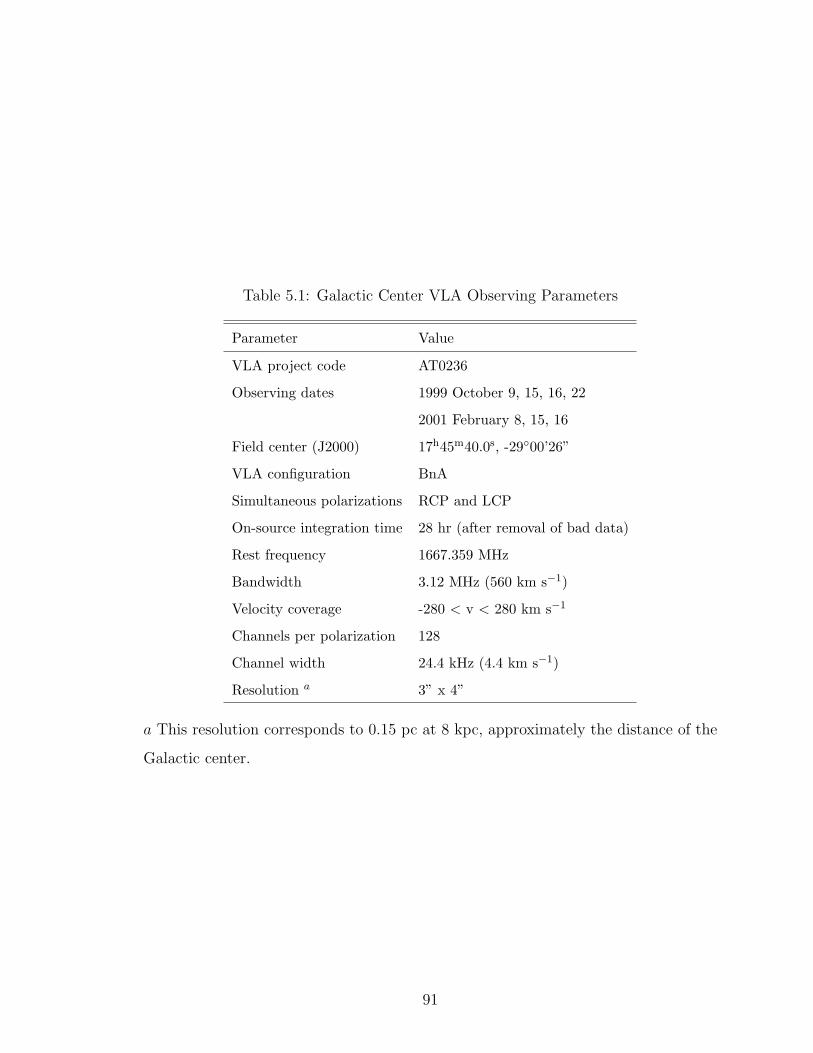
Table 5.1: Galactic Center VLA Observing Parameters

Parameter Value

VLA project code AT0236

Observing dates 1999 October 9, 15, 16, 22

2001 February 8, 15, 16

Field center (J2000) 17h45m40.0s, -29◦00’26”

VLA configuration BnA

Simultaneous polarizations RCP and LCP

On-source integration time 28 hr (after removal of bad data)

Rest frequency 1667.359 MHz

Bandwidth 3.12 MHz (560 km s−1)

Velocity coverage -280 < v < 280 km s−1

Channels per polarization 128

Channel width 24.4 kHz (4.4 km s−1)

Resolution a 3” x 4”

a This resolution corresponds to 0.15 pc at 8 kpc, approximately the distance of the

Galactic center.

91

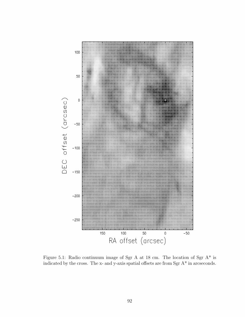
Figure 5.1: Radio continuum image of Sgr A at 18 cm. The location of Sgr A* isindicated by the cross. The x- and y-axis spatial offsets are from Sgr A* in arcseconds.

92

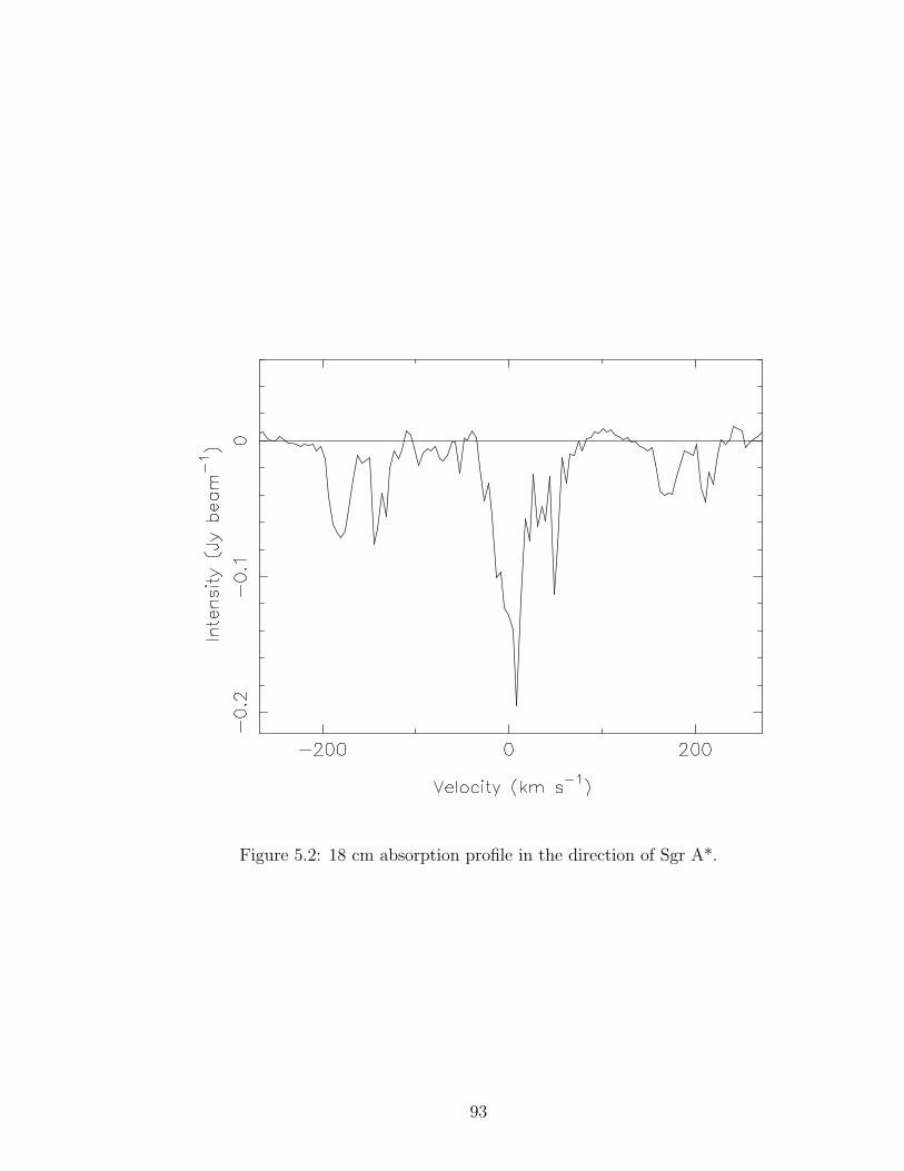
Figure 5.2: 18 cm absorption profile in the direction of Sgr A*.

93

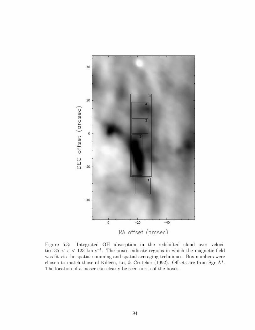
Figure 5.3: Integrated OH absorption in the redshifted cloud over veloci-ties 35 < v < 123 km s−1. The boxes indicate regions in which the magnetic fieldwas fit via the spatial summing and spatial averaging techniques. Box numbers werechosen to match those of Killeen, Lo, & Crutcher (1992). Offsets are from Sgr A*.The location of a maser can clearly be seen north of the boxes.

94

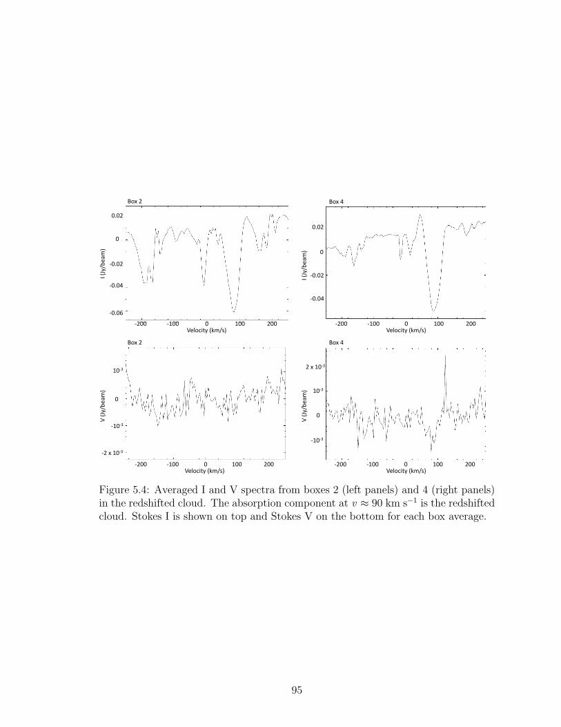
0

0.02

-0.04

-0.02

-0.06

0 100 200 -100 -200

Box 2

Velocity (km/s)

I (Jy

/bea

m)

0

0.02

0 100 200 -100 -200 Velocity (km/s)

I (Jy

/bea

m)

Box 4

-0.02

-0.04

0

10-3

-2 x 10-3

0 100 200 -100 -200 Velocity (km/s)

V (

Jy/b

eam

)

Box 2

-10-3

0

10-3

2 x 10-3

-10-3

0 100 200 -100 -200 Velocity (km/s)

V (

Jy/b

eam

)

Box 4

Figure 5.4: Averaged I and V spectra from boxes 2 (left panels) and 4 (right panels)in the redshifted cloud. The absorption component at v ≈ 90 km s−1 is the redshiftedcloud. Stokes I is shown on top and Stokes V on the bottom for each box average.

95

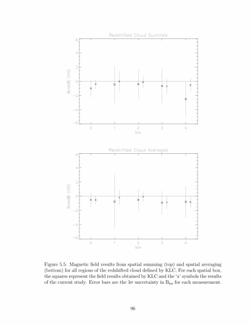
Figure 5.5: Magnetic field results from spatial summing (top) and spatial averaging(bottom) for all regions of the redshifted cloud defined by KLC. For each spatial box,the squares represent the field results obtained by KLC and the ‘x’ symbols the resultsof the current study. Error bars are the 3σ uncertainty in Blos for each measurement.

96

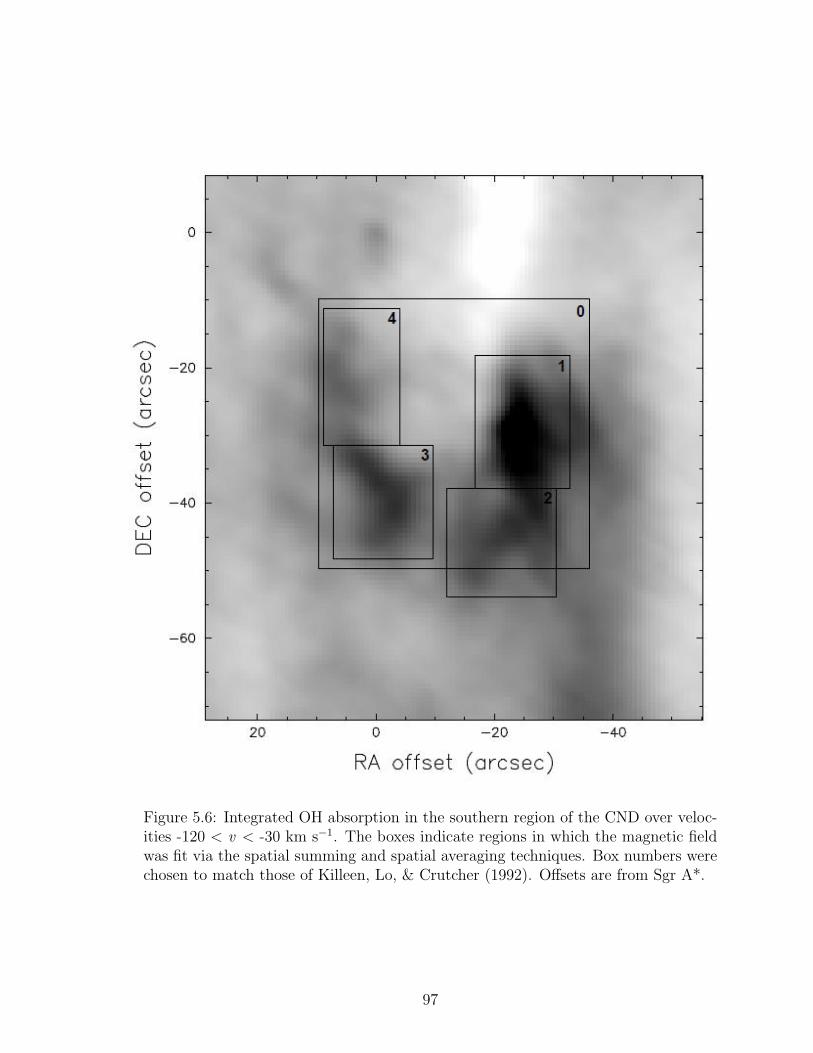
Figure 5.6: Integrated OH absorption in the southern region of the CND over veloc-ities -120 < v < -30 km s−1. The boxes indicate regions in which the magnetic fieldwas fit via the spatial summing and spatial averaging techniques. Box numbers werechosen to match those of Killeen, Lo, & Crutcher (1992). Offsets are from Sgr A*.

97

0

0.02

-0.04

0 100 200 -100 -200 Velocity (km/s)

I (Jy

/bea

m)

Box 1

-0.02

0

0.02

-0.06

0 100 200 -100 -200 Velocity (km/s)

I (Jy

/bea

m)

Box 3

-0.02

-0.04

0

2 x 10-3

10-3

-2 x 10-3 0 100 200 -100 -200

Velocity (km/s)

V (

Jy/b

eam

)

Box 1

-10-3

0

10-3

2 x 10-3

-10-3

0 100 200 -100 -200 Velocity (km/s)

V (

Jy/b

eam

)

Box 3

Figure 5.7: Averaged I and V spectra from boxes 1 (left panels) and 3 (right panels)in the southern region of the CND. Stokes I is shown on top and Stokes V on thebottom for each box average.

98

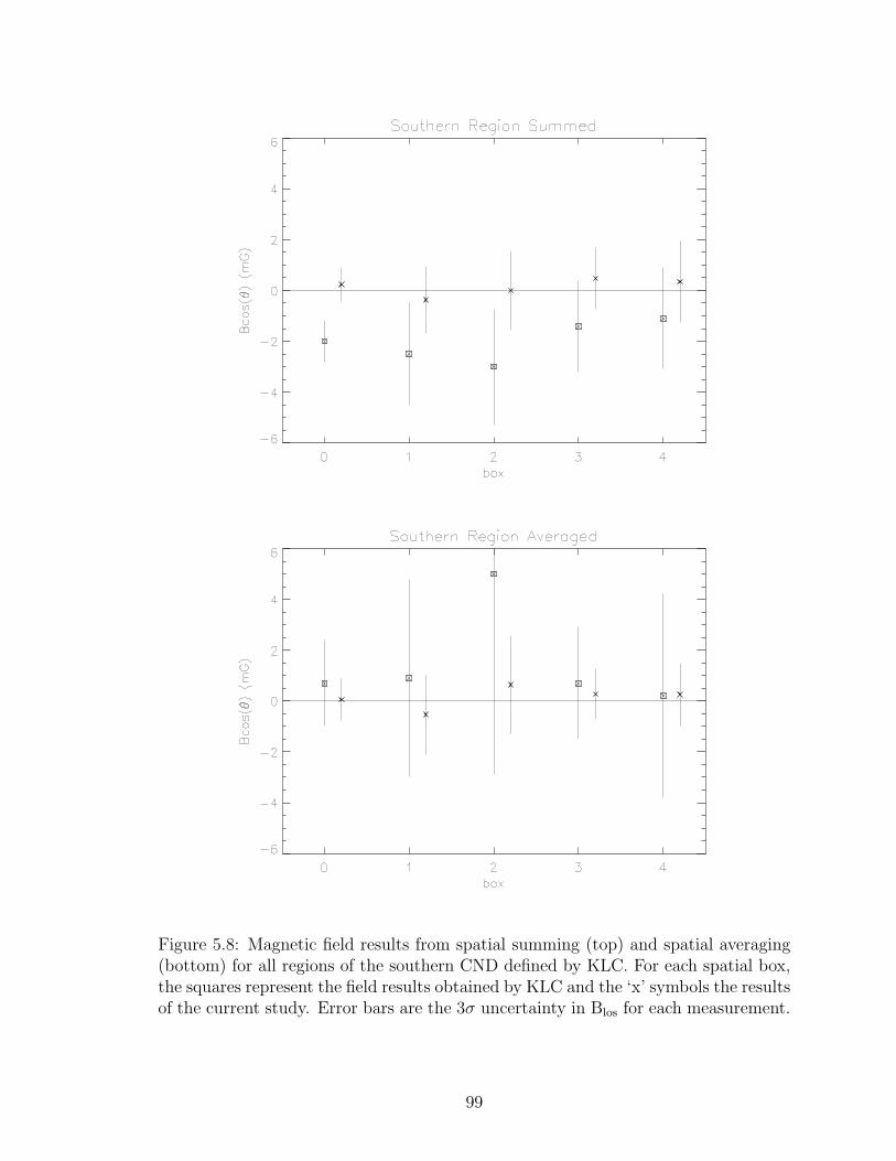
Figure 5.8: Magnetic field results from spatial summing (top) and spatial averaging(bottom) for all regions of the southern CND defined by KLC. For each spatial box,the squares represent the field results obtained by KLC and the ‘x’ symbols the resultsof the current study. Error bars are the 3σ uncertainty in Blos for each measurement.

99

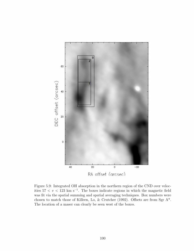
Figure 5.9: Integrated OH absorption in the northern region of the CND over veloc-ities 57 < v < 123 km s−1. The boxes indicate regions in which the magnetic fieldwas fit via the spatial summing and spatial averaging techniques. Box numbers werechosen to match those of Killeen, Lo, & Crutcher (1992). Offsets are from Sgr A*.The location of a maser can clearly be seen west of the boxes.

100

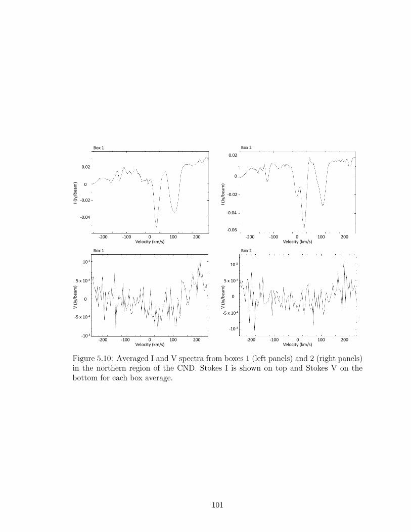
0

0.02

-0.04

-0.02

0 100 200 -100 -200 Velocity (km/s)

I (Jy

/bea

m)

Box 1

0

0.02

-0.06

0 100 200 -100 -200 Velocity (km/s)

I (Jy

/bea

m)

Box 2

-0.02

-0.04

0

5 x 10-4

10-3

-5 x 10-4

0 100 200 -100 -200 Velocity (km/s)

V (

Jy/b

eam

)

Box 1

-10-3

0

5 x 10-4

10-3

-5 x 10-4

0 100 200 -100 -200 Velocity (km/s)

V (

Jy/b

eam

)

Box 2

-10-3

Figure 5.10: Averaged I and V spectra from boxes 1 (left panels) and 2 (right panels)in the northern region of the CND. Stokes I is shown on top and Stokes V on thebottom for each box average.

101

Figure 5.11: Magnetic field results from spatial summing (top) and spatial averaging(bottom) for all regions of the northern CND defined by KLC. For each spatial box,the squares represent the field results obtained by KLC and the ‘x’ symbols the resultsof the current study. Error bars are the 3σ uncertainty in Blos for each measurement.

102

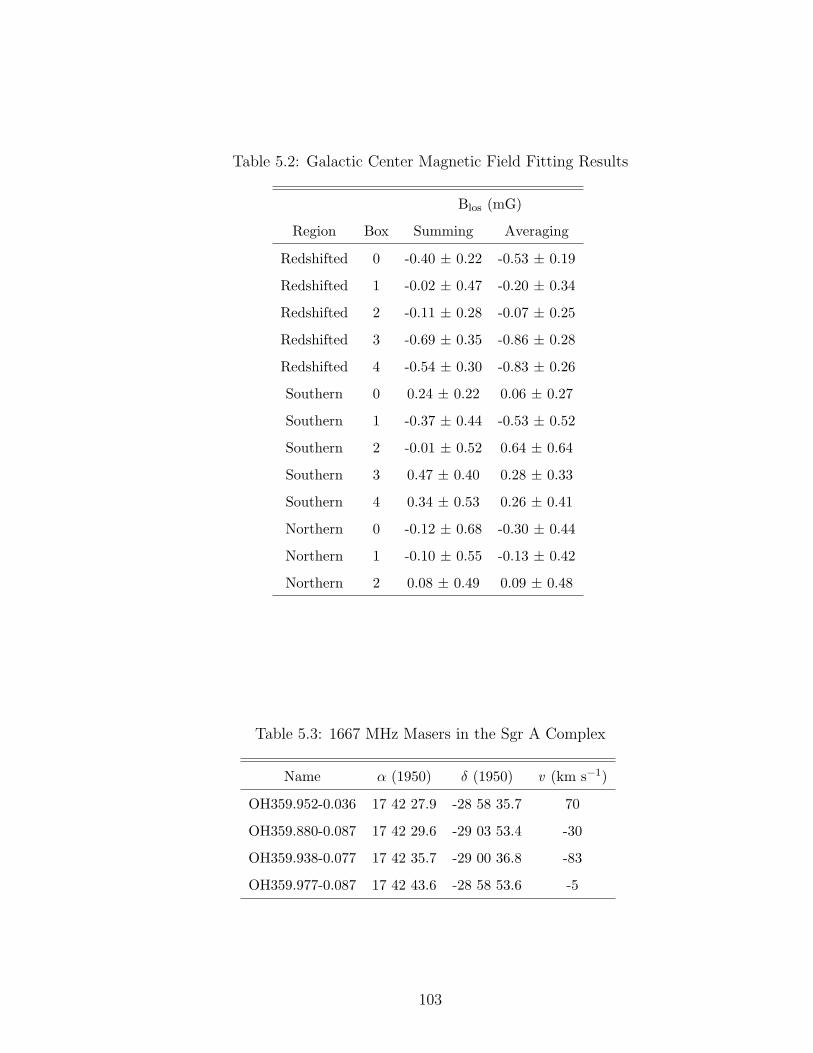
Table 5.2: Galactic Center Magnetic Field Fitting Results

Blos (mG)

Region Box Summing Averaging

Redshifted 0 -0.40 ± 0.22 -0.53 ± 0.19

Redshifted 1 -0.02 ± 0.47 -0.20 ± 0.34

Redshifted 2 -0.11 ± 0.28 -0.07 ± 0.25

Redshifted 3 -0.69 ± 0.35 -0.86 ± 0.28

Redshifted 4 -0.54 ± 0.30 -0.83 ± 0.26

Southern 0 0.24 ± 0.22 0.06 ± 0.27

Southern 1 -0.37 ± 0.44 -0.53 ± 0.52

Southern 2 -0.01 ± 0.52 0.64 ± 0.64

Southern 3 0.47 ± 0.40 0.28 ± 0.33

Southern 4 0.34 ± 0.53 0.26 ± 0.41

Northern 0 -0.12 ± 0.68 -0.30 ± 0.44

Northern 1 -0.10 ± 0.55 -0.13 ± 0.42

Northern 2 0.08 ± 0.49 0.09 ± 0.48

Table 5.3: 1667 MHz Masers in the Sgr A Complex

Name α (1950) δ (1950) v (km s−1)

OH359.952-0.036 17 42 27.9 -28 58 35.7 70

OH359.880-0.087 17 42 29.6 -29 03 53.4 -30

OH359.938-0.077 17 42 35.7 -29 00 36.8 -83

OH359.977-0.087 17 42 43.6 -28 58 53.6 -5

103

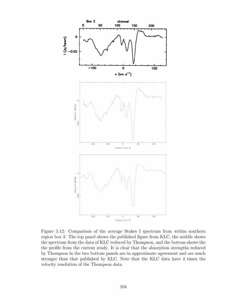
Figure 5.12: Comparison of the average Stokes I spectrum from within southernregion box 3. The top panel shows the published figure from KLC, the middle showsthe spectrum from the data of KLC reduced by Thompson, and the bottom shows thethe profile from the current study. It is clear that the absorption strengths reducedby Thompson in the two bottom panels are in approximate agreement and are muchstronger than that published by KLC. Note that the KLC data have 4 times thevelocity resolution of the Thompson data.

104

Chapter 6

Summary and Conclusions

6.1 Determination of the Mass-to-Flux Ratio in Molecular Clouds

We have conducted the first systematic observational survey to study the effect of

magnetic fields on molecular clouds as a whole. We have carried out 400 hours of

Arecibo Zeeman observations of OH absorption lines in the direction of Galactic

molecular clouds. The relevent parameter for determining the role of magnetic fields

in the star formation process is the mass-to-flux ratio λ, which observationally is pro-

portional to N/B, where N is the column density and B is the magnetic field strength.

A value of λ < 1 indicates a subcritical cloud dominated by magnetic energy, while a

value λ > 1 indicates a supercritical cloud dominated by gravity. The two competing

theories of star formation predict different ranges of values for λ. The turbulence-

driven theory requires magnetic fields that are too small to be dynamically important,

and predicts a broad range of lambda from 1 to 10 or more. The magnetically-driven

theory suggests that magnetic fields alone provide sufficient support against gravity

to slow the collapse of the cloud and subsequent star formation, requiring that λ is

less than or approximately equal to 1.

We have investigated 22 lines-of-sight through Galactic molecular clouds. Obser-

vations yield 5 Zeeman detections above the 3σ level in the direction of 3C092, 3C133,

4C+13.67, B1858+0407, and S88B. Magnetic field fitting results are given in Table

4.3. Since the Zeeman effect only reveals one component of the total field strength,

the results of the survey must be taken statistically. We find overall mean values of

Btot = 15.2 µG, N(H) = 4.5 x 1021 cm−2, and therefore λc = 1.5. We have assumed a

statistical correction of Btot = 2Blos and weighted the results by the inverse square of

the uncertainties in Blos. The mean mass-to-flux ratio of 1.5 suggests that the general

regions of molecular clouds are approximately critical to slightly supercritical. Such

a value cannot clearly distinguish between the two star formation theories.

105

Individual line-of-sight absorption components yield mass-to-flux ratio results for

which λ < 1, providing the first evidence for magnetically dominated molecular gas.

Although the results of the survey must be taken statically overall, we belive these

subcritical cloud detections are significant for two reasons. Firstly, the magnetic

field measurements involved in the calculation of λ for the subcritical measurements

are often field detections and are therefore considered to be trustworthy. Secondly,

the underestimate of field strength as a result of only measuring one component

of the total field produces an upper limit to the mass-to-flux ratio. The statistical

correction for the total strength would only act to lower λ and make the measurments

more subcritical. The turbulence-driven theory of star formation does not allow for

subcritical molecular gas, so these detections support only the magnetically-driven

theory.

We find that the mean visual extinction through the sampled molecular clouds

is approximately 2.4 magnitudes, nearly a factor of 3 lower than the value typically

quoted for GMCs. This means that our lines-of-sight are either preferentially sampling

regions of self-gravitating GMCs with lower than average densities or diffuse clouds

that have higher densities than average. The interpretation of our subcritical gas

measurements depends crucially on which scenario is correct. Our results appear

to be in agreement with the concept of magnetically supported clouds with column

densities a factor of 3 less than “standard” GMCs.

6.2 VLA Observations Toward the Sagittarius A Complex

Zeeman observations of 1667 MHz OH absorption lines in the direction of the Galac-

tic center were carried out using the BnA configuration of the VLA. The Zeeman

effect was unable to be detected in any individual synthesized beam. Application of

spatial averaging yielded marginal 3σ results of Blos = -0.53 ± 0.19, -0.86 ± 0.28,

and -0.83 ± 0.26 mG in the redshifted cloud region. These results are in general

agreement with negative milligauss fields suggested by other studies.

However, although our data have nearly 4 times the Zeeman sensitivity of the

previous study of Killeen, Lo, & Crutcher (1992), we are unable to confirm a 7σ and

106

multiple 4σ Zeeman detections reported by the authors. In addition, retrival and

reduction of the original data from the previous study does not reveal the significant

detections of the previous authors. We also find that the absorption line strengths in

both the current observations and the newly reduced archival data from the previous

study do not match the published results. We find comparable absorption line shapes,

but strengths that are consistantly approximately 1.7 times those published. We

have applied several consistency checks to ensure that our data reduction technique

is correct, each of which is discussed in Section 5.6. We therefore belive that the

results of the current study are accurate, and higher sensitivity measurements are

needed to constrain field strengths in the Sgr A complex of the Galactic center.

Copyright c© Kristen Lynn Thompson, 2012.

107

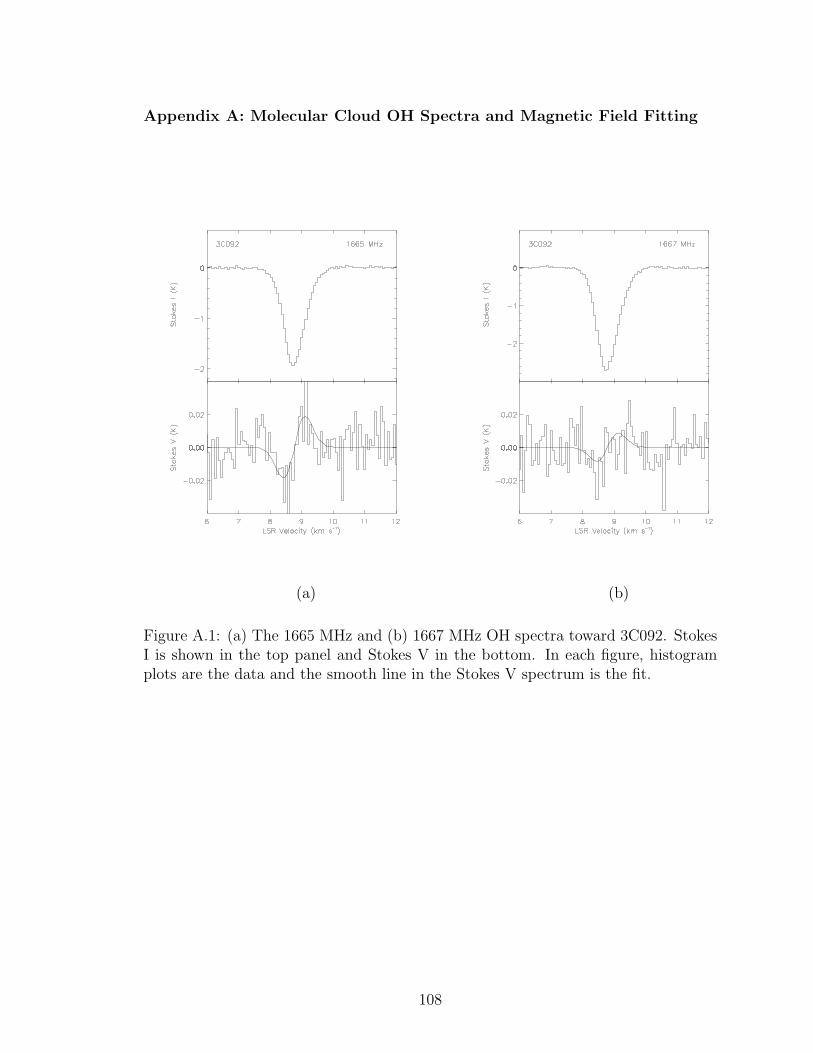
Appendix A: Molecular Cloud OH Spectra and Magnetic Field Fitting

(a) (b)

Figure A.1: (a) The 1665 MHz and (b) 1667 MHz OH spectra toward 3C092. StokesI is shown in the top panel and Stokes V in the bottom. In each figure, histogramplots are the data and the smooth line in the Stokes V spectrum is the fit.

108

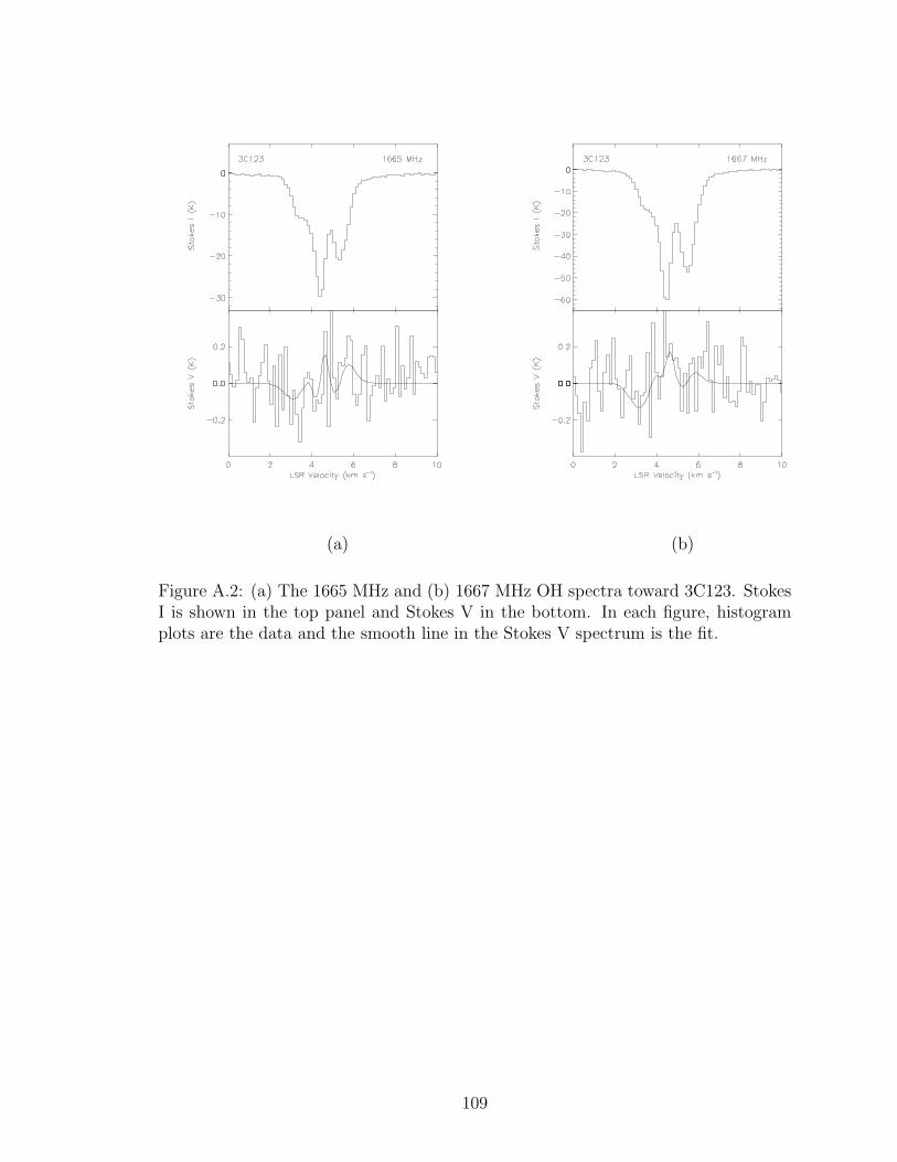
(a) (b)

Figure A.2: (a) The 1665 MHz and (b) 1667 MHz OH spectra toward 3C123. StokesI is shown in the top panel and Stokes V in the bottom. In each figure, histogramplots are the data and the smooth line in the Stokes V spectrum is the fit.

109

(a) (b)

Figure A.3: (a) The 1665 MHz and (b) 1667 MHz OH spectra toward 3C131. StokesI is shown in the top panel and Stokes V in the bottom. In each figure, histogramplots are the data and the smooth line in the Stokes V spectrum is the fit.

110

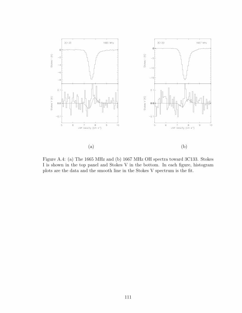
(a) (b)

Figure A.4: (a) The 1665 MHz and (b) 1667 MHz OH spectra toward 3C133. StokesI is shown in the top panel and Stokes V in the bottom. In each figure, histogramplots are the data and the smooth line in the Stokes V spectrum is the fit.

111

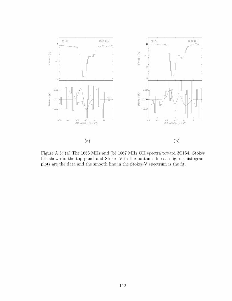
(a) (b)

Figure A.5: (a) The 1665 MHz and (b) 1667 MHz OH spectra toward 3C154. StokesI is shown in the top panel and Stokes V in the bottom. In each figure, histogramplots are the data and the smooth line in the Stokes V spectrum is the fit.

112

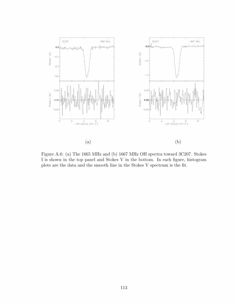
(a) (b)

Figure A.6: (a) The 1665 MHz and (b) 1667 MHz OH spectra toward 3C207. StokesI is shown in the top panel and Stokes V in the bottom. In each figure, histogramplots are the data and the smooth line in the Stokes V spectrum is the fit.

113

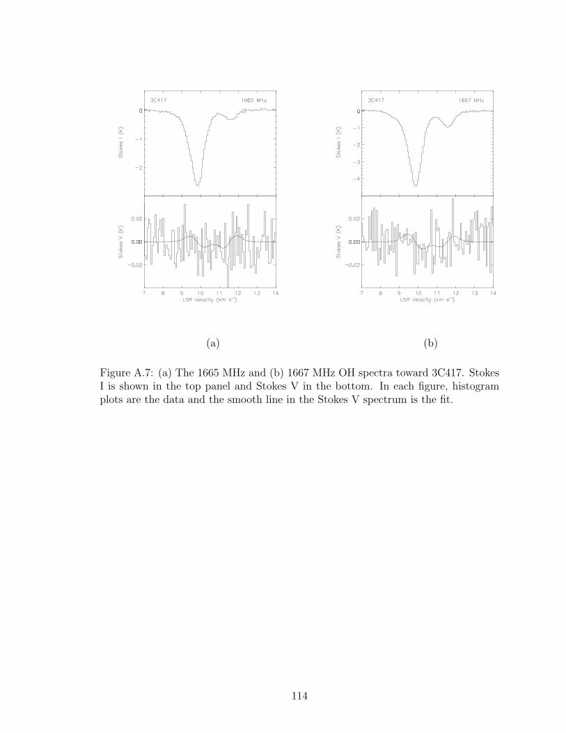
(a) (b)

Figure A.7: (a) The 1665 MHz and (b) 1667 MHz OH spectra toward 3C417. StokesI is shown in the top panel and Stokes V in the bottom. In each figure, histogramplots are the data and the smooth line in the Stokes V spectrum is the fit.

114

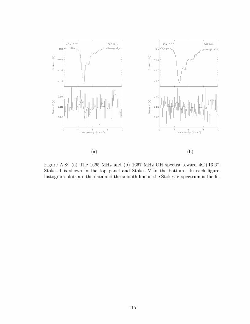
(a) (b)

Figure A.8: (a) The 1665 MHz and (b) 1667 MHz OH spectra toward 4C+13.67.Stokes I is shown in the top panel and Stokes V in the bottom. In each figure,histogram plots are the data and the smooth line in the Stokes V spectrum is the fit.

115

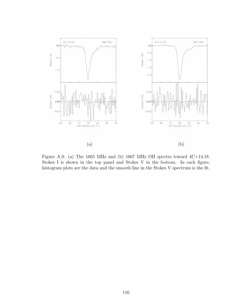
(a) (b)

Figure A.9: (a) The 1665 MHz and (b) 1667 MHz OH spectra toward 4C+14.18.Stokes I is shown in the top panel and Stokes V in the bottom. In each figure,histogram plots are the data and the smooth line in the Stokes V spectrum is the fit.

116

(a) (b)

Figure A.10: (a) The 1665 MHz and (b) 1667 MHz OH spectra toward 4C+17.23.Stokes I is shown in the top panel and Stokes V in the bottom. In each figure,histogram plots are the data and the smooth line in the Stokes V spectrum is the fit.

117

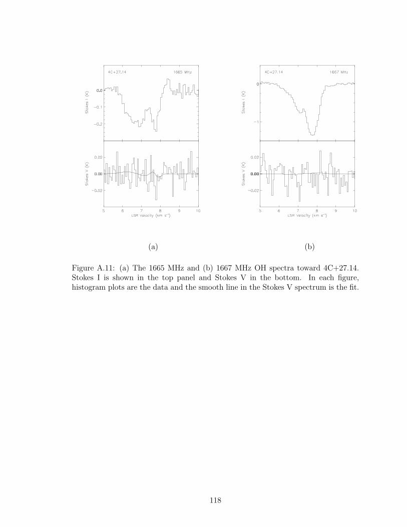
(a) (b)

Figure A.11: (a) The 1665 MHz and (b) 1667 MHz OH spectra toward 4C+27.14.Stokes I is shown in the top panel and Stokes V in the bottom. In each figure,histogram plots are the data and the smooth line in the Stokes V spectrum is the fit.

118

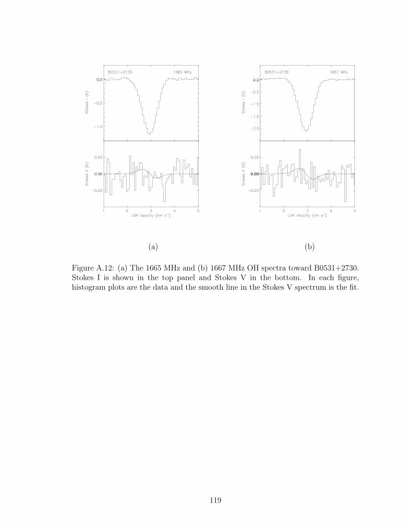
(a) (b)

Figure A.12: (a) The 1665 MHz and (b) 1667 MHz OH spectra toward B0531+2730.Stokes I is shown in the top panel and Stokes V in the bottom. In each figure,histogram plots are the data and the smooth line in the Stokes V spectrum is the fit.

119

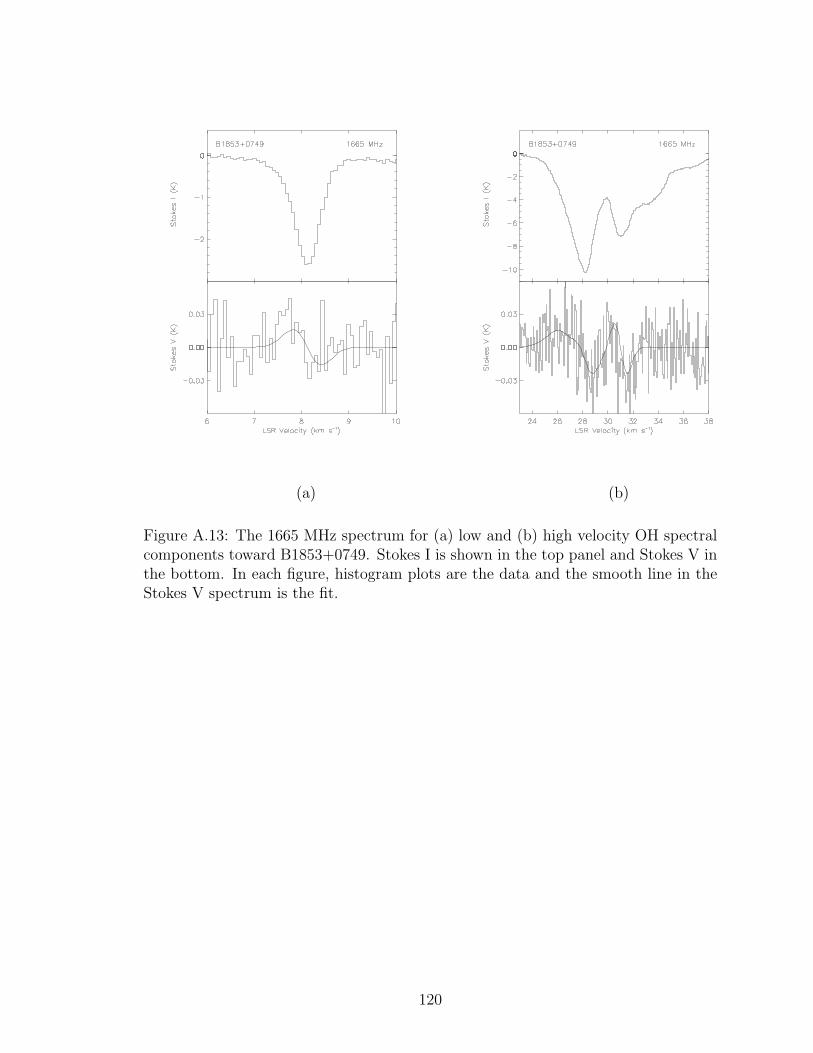
(a) (b)

Figure A.13: The 1665 MHz spectrum for (a) low and (b) high velocity OH spectralcomponents toward B1853+0749. Stokes I is shown in the top panel and Stokes V inthe bottom. In each figure, histogram plots are the data and the smooth line in theStokes V spectrum is the fit.

120

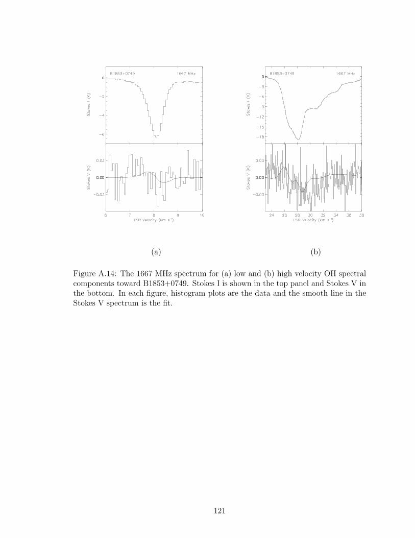
(a) (b)

Figure A.14: The 1667 MHz spectrum for (a) low and (b) high velocity OH spectralcomponents toward B1853+0749. Stokes I is shown in the top panel and Stokes V inthe bottom. In each figure, histogram plots are the data and the smooth line in theStokes V spectrum is the fit.

121

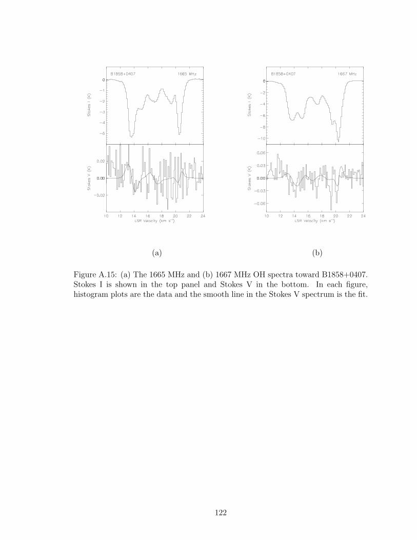
(a) (b)

Figure A.15: (a) The 1665 MHz and (b) 1667 MHz OH spectra toward B1858+0407.Stokes I is shown in the top panel and Stokes V in the bottom. In each figure,histogram plots are the data and the smooth line in the Stokes V spectrum is the fit.

122

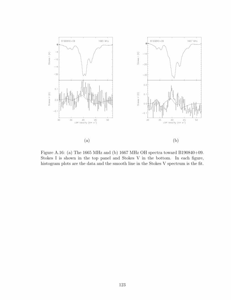
(a) (b)

Figure A.16: (a) The 1665 MHz and (b) 1667 MHz OH spectra toward B190840+09.Stokes I is shown in the top panel and Stokes V in the bottom. In each figure,histogram plots are the data and the smooth line in the Stokes V spectrum is the fit.

123

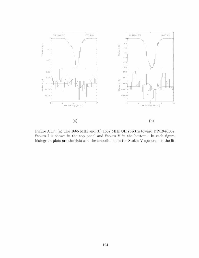
(a) (b)

Figure A.17: (a) The 1665 MHz and (b) 1667 MHz OH spectra toward B1919+1357.Stokes I is shown in the top panel and Stokes V in the bottom. In each figure,histogram plots are the data and the smooth line in the Stokes V spectrum is the fit.

124

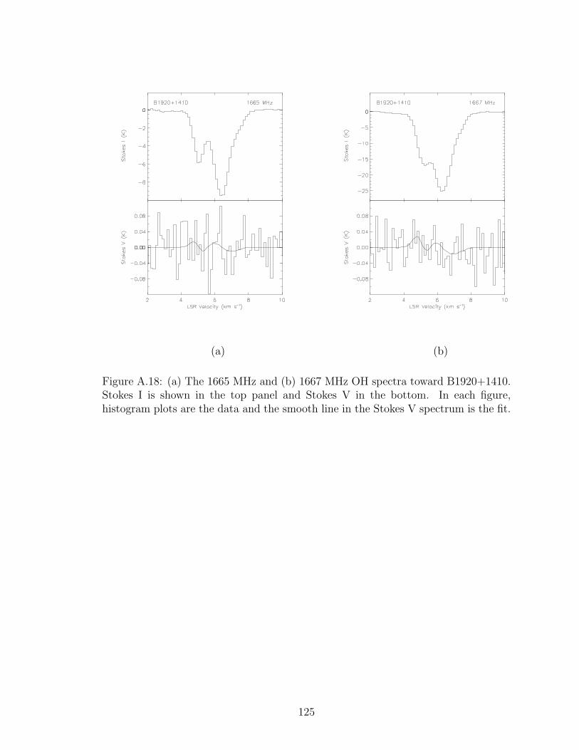
(a) (b)

Figure A.18: (a) The 1665 MHz and (b) 1667 MHz OH spectra toward B1920+1410.Stokes I is shown in the top panel and Stokes V in the bottom. In each figure,histogram plots are the data and the smooth line in the Stokes V spectrum is the fit.

125

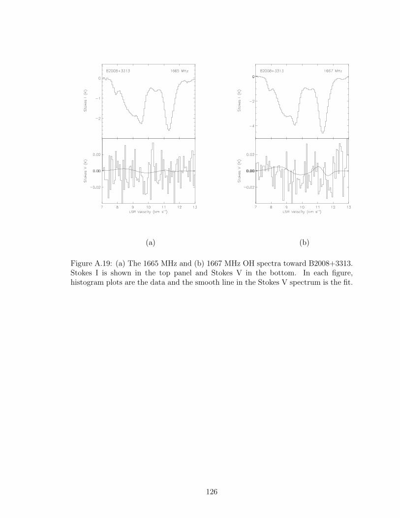
(a) (b)

Figure A.19: (a) The 1665 MHz and (b) 1667 MHz OH spectra toward B2008+3313.Stokes I is shown in the top panel and Stokes V in the bottom. In each figure,histogram plots are the data and the smooth line in the Stokes V spectrum is the fit.

126

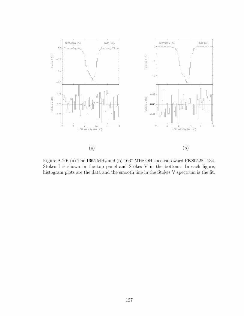
(a) (b)

Figure A.20: (a) The 1665 MHz and (b) 1667 MHz OH spectra toward PKS0528+134.Stokes I is shown in the top panel and Stokes V in the bottom. In each figure,histogram plots are the data and the smooth line in the Stokes V spectrum is the fit.

127

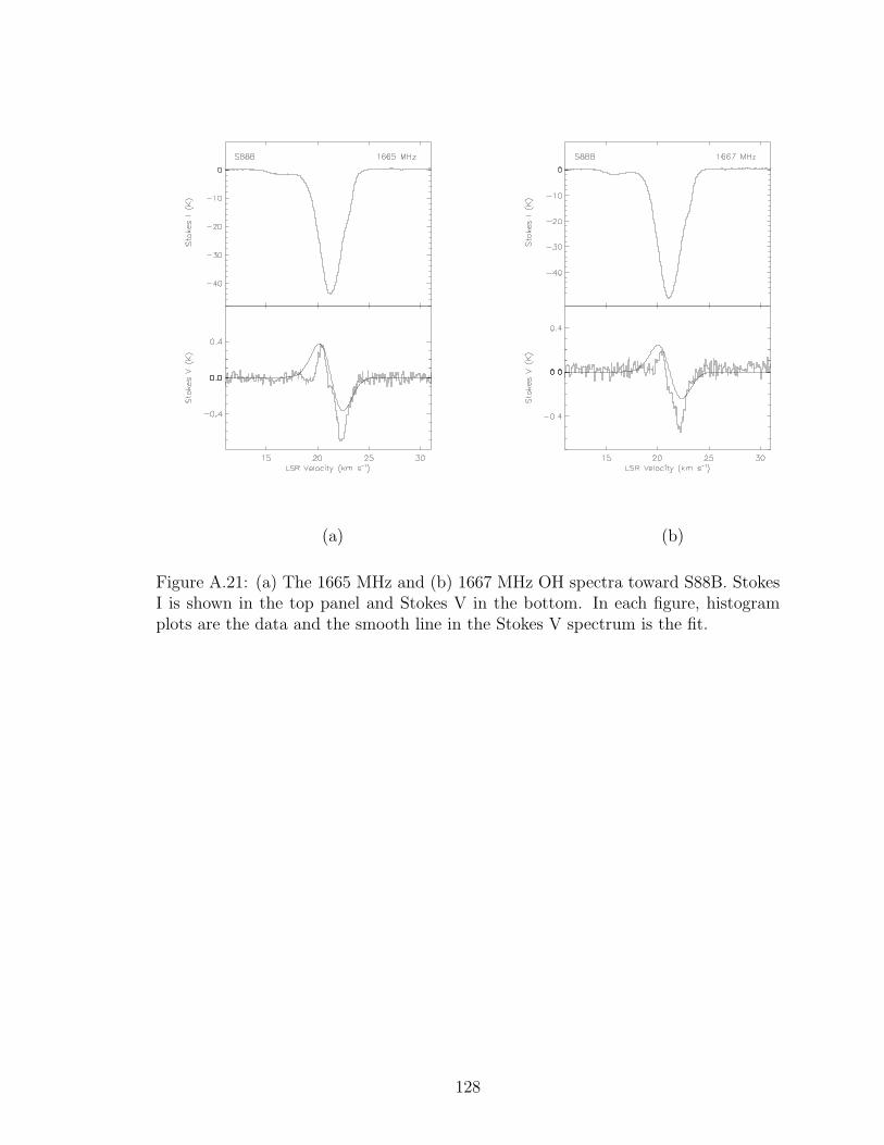
(a) (b)

Figure A.21: (a) The 1665 MHz and (b) 1667 MHz OH spectra toward S88B. StokesI is shown in the top panel and Stokes V in the bottom. In each figure, histogramplots are the data and the smooth line in the Stokes V spectrum is the fit.

128

(a) (b)

Figure A.22: (a) The 1665 MHz and (b) 1667 MHz OH spectra toward T0629+10.Stokes I is shown in the top panel and Stokes V in the bottom. In each figure,histogram plots are the data and the smooth line in the Stokes V spectrum is the fit.

129

Bibliography

Aitken, D.K., Gezari, D., Smith, C.H., McCaughrean, M., & Roche, P.F. 1991, ApJ,

380, 419

Blitz, L., & Williams, J.P. 1999, in The Origin of Stars and Planetary Systems, ed.

C.J. Lada, & N.D. Kylafis (Dordrecht: Kluwer), 3

Bohlin, R.C., Savage, B.D., & Drake, J.F. 1978, ApJ, 224, 132

Bourke, T.L., Myers, P.C., Robinson, G., & Hyland, A.R. 2001, ApJ, 554, 916

Clemens, D.P. 1985, ApJ, 295, 422

Coles, W.A., & Rumsey, V.H. 1970, ApJ, 159, 247

Condon, J.J., et al. 1998, AJ, 115, 1693

Crutcher, R.M. 1977, ApJ, 216, 308

Crutcher, R.M. 1979, ApJ, 234, 881

Crutcher, R.M., Heiles, C., & Troland, T.H. 1981, 249, 134

Crutcher, R.M. 1999, ApJ, 520, 706

Crutcher, R.M., & Troland, T.H. 2000, ApJ, 537, L139

Crutcher, R.M. 2007, in Magnetic Fields in Molecular Clouds. EAS Publications

Series, 23, 37

Crutcher, R.M., Wandelt, B., Heiles, C., Falgarone, E., & Troland, T.H. 2010, ApJ,

725, 466

Crutcher, R.M. 2012, ARA&A, 50, 29

Dame, T.M., Hartmann, D., & Thaddeus, P. 2001, ApJ, 547, 792

130

Draine, B.T., 2011, Physics of the Interstellar and Intergalactic Medium (Princeton

series in astrophysics), 5

Eisenhauer, F. et al. 2003, ApJ, 597, L121

Ekers, R.D., van Forkom, J.H., Schwarz, U.J., & Goss, W.M. 1983, A&A, 122, 143

Falgaron, E., Troland, T.H., Crutcher, R.M., & Paubert, G. 2008, A&A, 487, 247

Field, G.B., Goldsmith, D.W., & Habing, H.J. 1969, ApJ, 155, L149

Gillessen, S. 2009, ApJ, 692, 1075

Goodman, A.A., Crutcher, R.M., Heiles, C., Myers, P.C., & Troland, T.H. 1989, ApJ,

338, L61

Gusten, R., Downes, D. 1981, A&A, 99, 27

Gusten, R., Genzel, R., Wright, M.C.H., Jaffe, D.T., Stutzki, J., & Harris, A.I. 1987,

ApJ, 318, 124

Han, J. L. 2008, Nucl. Phys. B Proc. Suppl., 175, 62

Hartquist, T.W., & Williams, D.A. 1989, MNRAS, 241, 417

Heiles, C., & Stevens, M. 1986, ApJ, 301, 331

Heiles, C., & Troland, T.H. 2003a, ApJS, 145, 329

Heiles, C., & Troland, T.H. 2003b, ApJ, 586, 1067

Heiles, C., & Troland, T.H. 2004, 151, 271

Heiles, C., & Troland, T.H. 2005, 624, 773

Karlsson, R., Sjouwerman, L.O., Sandqvist, Aa., & Whiteoak, J.B. 2003, A&A, 403,

1011

Kemper, F., Vriend, W.J., & Tielens, A.G.G.M. 2005, ApJ, 633, 534

131

Killeen, N.E.B., Lo, K.Y., & Crutcher, R. 1992, ApJ, 385, 585

Lindqvist, M., Winnberg, A., Habing, H.J., & Matthew, H.E. 1992, A&AS, 92, 43

(L-92)

Liszt, H.S., & Burton, W.B. 1993, ApJ, 407, L25

Lo, K.Y., & Claussen, M.J. 1983, Nature, 306, 647

Mac Low, M.-M., & Klessen, R.S. 2004, Rev. Mod. Phys., 76, 125

McKee, C.F., 1999, in The Origin of Stars and Planetary Systems, ed. C.J. Lada &

N.D. Kylafis (Dordrecht: Kluwer), 29

McKee, C.F., Zweibel, E.G., Goodman, A.A., & Heiles, C. 1993, in Protostars and

Planets III, ed. E.H. Levy & J.I. Lunine (Tucson: Univ. Arizona Press), 327

Mouschovias, T.Ch, & Spitzer, L. 1976, ApJ, 201, 326

Mouschovias, T.Ch, & Morton, S.A. 1991, ApJ, 371, 296

Plante, R.L., Lo, K.Y., & Crutcher, R.M. 1995, ApJ, 445, L113

Reid, M.J. 1993, ARA&A, 31, 345

Rieke, G.H., & Lebofsky, M.J. 1985, ApJ, 288, 618

Roberts, D.A., Crutcher, R.M., & Troland, T.H. 1995, ApJ, 442, 208

Robinson B. J., McGee R. X. 1967, ARA&A, 5, 183

Sault, R.J., Killeen, N.E.B., Zmuidzinas, J., & Loushin, R. 1990, ApJS, 74, 437

Shu, F.H., Allen, A., Shang, H., Ostriker, E., & Li, Z-Y. 1999, in The Origin of Stars

and Planetary Systems, ed. C.J. Lada & N.D. Kylafis (Dordrecht: Kluwer), 193

Sofue, Y., Reich, W., Inoue, M., & Seiradakis, J.H. 1987, PASJ, 39, 95

Spitzer, L., Jr. 1978, Physical Processes in the Interstellar Medium (New York: Wiley)

132

Tomisake, K., Ikeuchi, S., & Nakamura, T. 1988, ApJ, 335, 239

Troland, T.H. 1990, in Galactic and Intergalactic Magnetic Fields, ed. R. Beck, R.

Wielebinski, & P. Kronberg (Dordrecht: Kluwer), 293

Troland, T.H., & Crutcher, R.M. 2008, ApJ, 680, 457

Tsuboi,M., Inoue, M., Handa, T., Tabara, H., Kato, T., Sofue, Y., & Kaifu, N. 1986,

AJ, 92, 818

Weinreb, S., Barrett, A.H., Meeks, M.L., & Henry, J.C. 1963, Nature, 200, 829

Wegner, W. 2003, Astron. Nachr., 324, 219

Yusef-Zadeh, F., Roberts, D.A., Goss, W.M., Frail, D.A., & Green, A.J. 1996, ApJ,

466, L25

Yusef-Zadeh, F., Hewitt, J.W., & Cotton, W. 2004, ApJS, 155, 421Y

Zhao, J-H, Goss, W.M., & Ho, P.T.P. 1995, ApJ, 450, 122

133

VITA

Kristen L. Thompson

• Date and place of birth:

– September 30, 1984; East Liverpool, Ohio

• Educational institutions attended and degrees awarded:

– M.S. in Physics & Astronomy, University of Kentucky, 2009

– B.S. in Physics & Astronomy, Mount Union College, 2006

• Professional positions held:

– Instructor, Bluegrass Community and Technical College, 2010-2012

– Research Assistant, University of Kentucky, 2009-2012

– Graduate Assistant for MacAdam Student Observatory, University of Ken-

tucky, 2007-2009

– Intern, National Radio Astronomy Observatory, 2006

– NSF REU Program, National Radio Astronomy Observatory, 2006

– NSF REU Program, Bucknell University, 2005

• Scholastic and professional honors:

– Valedictorian, Southern Local High School, Salineville, Ohio, 2002

– American Astronomical Society, member

– Pi Mu Epsilon, member

– Sigma Pi Sigma, member

134

• Professional publications

– “Interactions Between Forming Stars and Dense Gas in the Small Low-

Mass Cluster Cederblad 110” E. F. Ladd, T. Wong, T. L. Bourke, & K.

L. Thompson, 2011, ApJ, 743, 108

135