Zeeman effect

Max-Planck-Institut fur Kernphysik,

Saupfercheckweg 1, Heidelberg

March 10, 2012

Introduction

The most important experimental technique triggering the development of the mod-

ern atomic theory is spectroscopy, the observation of the characteristic wavelengths

of light that atoms can absorb and emit. A so-called wavelength dispersive element

such as a waterdrop, a prism or a grating, spatially separates different wavelengths

of light emitted from one source. If the light source emits white light, a band of all

colours will be found after the light passes the wavelength dispersive element (e.g.

rainbow). Observing the light from a lamp that contains only atoms of a certain

element, one finds distinct lines instead of the complete band on the detector. The

positioning of the lines on the detector is called a spectrum, and the corresponding

wavelengths are hence called ‘spectral lines’ of the element. The additional informa-

tion needed to be able to draw conclusions about the atomic structure from spectral

lines was provided by the experimental observation of Rutherford that in an atom,

electrons surround a heavy, positively charged nucleus in the center, and by Planck’s

explanation of the blackbody spectrum by quanta of light, photons, whose energy

Eph is connected with the wavelength λ by

Eph = hν =hc

λ, (1)

where ν is the frequency, h is the Planck constant and c is the speed of light. With

this knowledge it became clear that electrons in an atom can occupy only certain

energy levels Ei, and that the transition of an electron from a higher energy level

E2 to a lower energy level E1 leads to the emission of a photon: E2 − E1 = Eph.

The energy needed to lift the electron to the higher, ‘excited’ energy level can be

provided by absorption of a photon of the very same energy or by collisions.

The increasing experimental precision reached with spectroscopy inspired scientists

1

2

to propose different atomic models, leading to the development of quantum mechan-

ics. With refinements to the quantum mechanical description of the atom, relativis-

tic quantum mechanics (necessary to explain the the splitting of energy levels of

same main quantum number n) and quantum electrodynamics (QED, necessary to

explain the splitting of levels with same quantum number j but different quantum

number l), theory is by now able to make highly accurate predictions about the

atomic structure.

Effects of an external magnetic field on the atomic

structure

If the atom is placed in an external magnetic field, the

Figure 1: Classical model

of an electron with angu-

lar momentum l inducing

an angular magnetic mo-

ment ~µl

atomic energy levels are split and the observed spectrum

changes. This was first observed by the dutch physicist

Pieter Zeeman and is hence called the Zeeman effect.

In an intuitive approach to explain the Zeeman effect,

consider an atom with an electron with charge e moving

with the speed v around the nucleus on a Bohr orbit with

radius r. This orbiting electron can be described by a

current

I = −e · v

2πr(2)

inducing an orbital magnetic moment

~µl = I ·A = I · πr2n =evr

2n , (3)

where A = πr2n is the area vector perpendicular to the orbit area πr2. The angular

momentum of the electron with mass me is

l = r× p = me · r · v · n . (4)

An external magnetic field B interacts with the angular magnetic moment and,

hence, changes the electron’s potential energy:

∆Epot = −~µl ·B =e

2me

· l ·B (5)

Using the direction of the magnetic field vector B as quantisation axis z and the

quantised angular momentum of the electron

|l| =√l(l + 1)~ with l = 0, 1, . . . , n− 1 and (6)

lz = ml · ~ with − l ≤ ml ≤ l , (7)

3

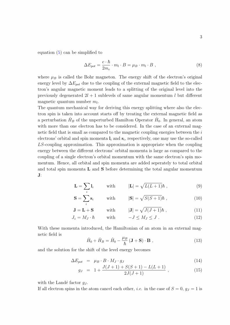
equation (5) can be simplified to

∆Epot =e · ~2me

·ml ·B = µB ·ml ·B , (8)

where µB is called the Bohr magneton. The energy shift of the electron’s original

energy level by ∆Epot due to the coupling of the external magnetic field to the elec-

tron’s angular magnetic moment leads to a splitting of the original level into the

previously degenerated 2l + 1 sublevels of same angular momentum l but different

magnetic quantum number ml.

The quantum mechanical way for deriving this energy splitting where also the elec-

tron spin is taken into account starts off by treating the external magnetic field as

a perturbation HB of the unperturbed Hamilton Operator H0. In general, an atom

with more than one electron has to be considered. In the case of an external mag-

netic field that is small as compared to the magnetic coupling energies between the i

electrons’ orbital and spin momenta li and si, respectively, one may use the so-called

LS-coupling approximation. This approximation is appropriate when the coupling

energy between the different electrons’ orbital momenta is large as compared to the

coupling of a single electron’s orbital momentum with the same electron’s spin mo-

mentum. Hence, all orbital and spin momenta are added seperately to total orbital

and total spin momenta L and S before determining the total angular momentum

J:

L =∑i

li with |L| =√L(L+ 1)~ , (9)

S =∑i

si with |S| =√S(S + 1)~ , (10)

J = L + S with |J| =√J(J + 1)~ , (11)

Jz = MJ · ~ with −J ≤MJ ≤ J . (12)

With these momenta introduced, the Hamiltonian of an atom in an external mag-

netic field is

H0 + HB = H0 −µB~

(J + S) ·B , (13)

and the solution for the shift of the level energy becomes

∆Epot = µB ·B ·MJ · gJ (14)

gJ = 1 +J(J + 1) + S(S + 1)− L(L+ 1)

2J(J + 1), (15)

with the Lande factor gJ .

If all electron spins in the atom cancel each other, i.e. in the case of S = 0, gJ = 1 is

4

Figure 2: Left: Normal Zeeman effect for a d → p transition. The field splits the

degenerate MJ levels by ∆E = µB ·B ·MJ . Right: Anomalous Zeeman effect. Here,

the levels are split by ∆E = µB ·B ·MJ · gJ . In both cases, transitions can occur if

∆mJ = 0,±1.

obtained and equation (14) becomes identical to equation (5). For historical reasons,

the splitting in absence of spin is called the normal Zeeman effect whereas, since the

electron spin was not yet discovered and the observed features seen in the spectra

were not understood, the more general case with S 6= 0 was named the anomalous

Zeeman effect. In the normal Zeeman effect, the size of the energy splitting from the

unperturbed level energy depends only on the magnetic quantum number ml and

is, hence, of the same size for all levels in the atom. In the case of the anomalous

Zeeman effect, the energy splitting depends on the quantum numbers J, L and S,

which is reflected by more complicated structures observed in the corresponding

spectra (see Fig. 2). In a strong external field, the LS-coupling approximation is

no longer appropriate. The field-induced precessions are so rapid that one has to

consider the total orbital momentum L and spin S as they individually precess about

B, that is, the effect of B is effectively to decouple L from S, rendering J meaningless.

This is called the Paschen-Back effect.

5

ps

ps

B

s+

s-

s+

s-

Figure 3: Isometric depiction of the polarisation of the different Zeeman compo-

nents.

Selection rules and polarisation of emitted light

In transitions from an excited level i to a lower level k, a photon with the difference

energy Eph = ∆E = Ei − Ek is emitted. Still, as indicated in Fig. 2, not all energy

differences between existing levels are actually found in the spectra. The reason

is that not only the energy, but also momentum conservation, angular momentum

conservation and symmetry rules play a role on whether or not a transition can occur.

Only those transitions are allowed where the transition dipole matrix element

Mik = e

∫ψ∗i r ψk dV (16)

has at least one non-zero component

(Mik)q = e

∫ψ∗i q ψk dq , with q = x, y, z . (17)

Evaluating these three integrals yields that only those transitions have non-zero

components where the change of the magnetic quantum number fulfills ∆MJ =

MJ,i−MJ,k = 0,±1. Furthermore, electric dipole transitions require that the change

of the total orbital momentum be ∆L = Li − Lk = ±1 and that the spin does not

change, i.e. ∆S = 0.

If the quantisation axis (i.e. the direction of the magnetic field vector) is the z-axis,

the matrix element component (Mik)z is the only non-zero one for ∆MJ = 0 (so-

called ‘π’-) transitions. Considering a dipole and its characteristics of emission, this

means the dipole is oscillating along the axis of the magnetic field vector and, hence,

does not emit any radiation in that direction. Also, since the electric field vector

is oscillating in only one direction, also the field vector of the emitted light wave

oscillates in this direction, meaning that the light emitted by ∆MJ = 0 transitions

6

is linearly polarised (see Fig. 3).

In the case of ∆MJ = ±1 (‘σ’-) transitions, (Mik)z is zero and both (Mik)x and

(Mik)y are non-zero and equal in magnitude, but phase-shifted by π/2. This phase

shift between the two superimposed dipoles leads to the observation of circularly

polarised light when viewing in z-direction (‘longitudinally’). Viewing the emitted

light in x- or y-direction (‘transversal’), only the projection of the superimposed

dipoles is seen, and thus the light from ∆MJ = ±1 transitions appears linearly

polarised when observed transversal to the magnetic field vector.

The Experiment

The experiment consists of two parts. In the first part, the Zeeman effect intransverse and longitudinal directions should be observed, and the polarisationof the observed lines examined. The second part is dedicated to precision spec-troscopy with a grating spectrometer. In both parts of the experiment the lightemitted from a Cadmium lamp (Cd) will be used. The electronic configurationof Cadmium is [Kr]4d105s2. In this configuration all spins of the shell electronscompensate for each other, such that S = 0. In visible light, the Cd spectrumconsists of four lines, given in table 1. All measurements will be made on the redline, λ0 = 643.8nm (ν0 = 465.7THz), which arises from the transition betweenthe two excited levels 1D2 →1 P1 in the fifth shell of Cd.

Colour violet blue green redWavelength (nm) 467.9 480.1 508.7 643.8

Table 1: Spectral lines of Cadmium in the visible range.

Part 1: Spectroscopy of the Zeeman Effect

As the expected relative shift in wavelength due to the external magnetic fieldis smaller than 0.1 nm, a very high resolution is necessary for the effect to beobservable. In this experiment the so-called Lummer-Gehrcke Plate will be used(see figure 1). This is a quartz glass plate with extremely plane parallel surfaces.The light enters into the plate through the use of a prism, and is then reflected toand fro between the innersurfaces of the plate under an angle near to total internalreflection. In this way, a small part of the light escapes from the plate at everypoint of reflection, under an angle of α ∼ 90◦ (to the normal of the plate). Theescaping rays of light can be observed with a telescope fixed behind the plate,whose focal point is at infinity. As the thickness of the plate is a lot smaller thanits length and additionally this has a higher coefficient of reflection, many lightrays can interfere with one another. This leads to a very high resolution. As canbe seen in figure 1, the optical path length difference between two light rays, oneof which is delayed by the glass plate, is given by:

∆ = 2n2 ·d

cosε− 2n1 · d · tan ε · sinα , (1)

with the thickness of the plate d, the indices of refraction (braking indices) n1

and n2 outside and inside the place, and similarly with the angles of the light raysto the normal of the plate (outside and inside the plate) α and ε. With sinα =n2

n1sin ε and sin2 ε+ cos2 ε = 1 equation 1 becomes:

∆ = 2n2 · d · cos ε = 2 · d ·√n2

2 − n21 sin2 α . (2)

1

Figure 1: Schematic of the Lummer-Gehrcke-Plate

In the case of the Lummer-Gehrcke plate, the light is introduced into the platethrough a prism, such that α ∼ 90◦ at the limit of total internal reflection. For aplate with n2 ∼ n in air, (n1 ∼ 1) equation 2 reduces to:

∆ = ∆1 −∆2 = 2d ·√n2 − 1 . (3)

where the ∆i are marked in the right hand part of diagram 1. For constructiveinterference the path difference must satisfy ∆ = m ·λ, with k as a whole numberand the wavelength λ of the interfering light. Whether constructive or destructiveinterference occurs when the Lummer-Gehrcke Plate is observed with the tele-scope, depends on the wavelength λ, the escape angle α and hence also on theangle β under which the light enters the plate. For a given wavelength λ one re-covers many orders k for different entering angles β at which the escaping lightrays interfere constructively (compare diagram 2). The order k of wavelengthλ+ ∆λ and order k + 1 of wavelength λ overlap spatially when

k · (λ+ ∆λ) = (k + 1) · λ→ ∆λ =λ

k. (4)

With equation 3 the free spectral range of the Lummer-Gehrcke-Plate followsfrom

∆λ =λ2

2d ·√n2 − 1

. (5)

To a first approximation, a small change in wavelength δλ � ∆λ leads to a shiftof

δλ =δa

∆a·∆λ , (6)

2

Figure 2: Interference pattern for the Zeeman effect, as would be observed in the trans-verse direction for the case a) without polarisation filter, b) with polarisation direction ofthe filter perpendicular to the magnetic field and c) with polarisation direction of the filterparallel to the magnetic field.

with the distance δa between the line with wavelength λ+ δλ and the positionof the line with wavelength λ, and the distance ∆a between two orders k and k+1of wavelength λ. Therefore, for small shifts in wavelength as is the case for theZeeman effect, one obtains the following:

δλ =δa

∆a· λ2

2d ·√n2 − 1

. (7)

The experimental setup is sketched in figure 3. The Cd-lamp is placed betweenthe pole pieces of the magnet. Light emitted from this lamp enters the Lummer-Gehrcke plate after passing through the red filter. This filter only lets the red partof the Cd spectrum through. The magnet can be turned through 90◦, so that thelamp can be observed in tranverse and longitudinal directions. The longitudinaldirection may be observed through the hole in the pole piece. The interferencepattern produced by the Lummer-Gehrcke plate can be observed through the tele-scope. In order to observe the different polarisations, a polarisation filter and a λ/4filter may be fixed between the plate and the telescope. With the height adjustmentof the telescope, a crosshair in the eyepiece can be moved over the interferencepattern.

3

Figure 3: Drawing of the experimental set-up for investigating the normal Zeeman effect(Figure from Leybold, Physics Leaflets). a) Pole pieces of the magnets, b) Cd lamp, c) Redlight filter, d) Lummer-Gehrcke Plate, e) Telescope, f) Eyepiece, g) Height adjustment forthe telescope, h) Locking screw for the telescope holder, i) Locking screw for the base.

Part 1: Execution (1-2 afternoons or a whole day)

• Use the teslameter (Hall probe) to determine the strength of the magneticfield at the position of the Cd-lamp. The magnetic field strength shouldbe measured as a function of the current through the power supply of themagnets. Carry out the measurements once with increasing and once withdecreasing current (Hysterisis effect). Take three measurements per currentvalue and average.

• Carefully set the Cd lamp into the holder with the magnetic field turned off(without using force!) and observe the Zeeman effect in transverse and lon-gitudinal directions with the telescope and with the camera. → Let turningthe magnets be demonstrated by the supervisor first!

• Use the polarisation filter and the λ/4 filter (how can the two be distin-guished?) in order to verify the polarisations of the different Zeeman com-ponents with different observation directions (transverse and longitudinal).

• Using the ScopePhoto program, record an impace of the σ− and π−linesfor 10-12 orders of interference k with currents for the magnetic field ofI = 10A, I = 12A and I = 14A.

• ScopePhoto program:

– Open program

– TC (bring up previews)

4

– Settings (optimise gain, select time)

– Capture (record a spectrum)

– File→ save as file:C/Practical/your names

• Open images from ScopePhoto in the program ImageJ to work on themthere.

• ImageJ program:

– Open image from ScopePhoto

– Image→ Colour→ RGB split→ (close blue and green)

– Mark lines on the image (zoom and center the end points of the line)

– PlugIns→ Spectroscopy→ Shift (produced from a projection of theimage)

– Save the image

Security Advice:

• The Lummer-Gehrcke plate and its cover may not be taken away. The plateis very expensive!

• The current for the magnetic field should always be turned off when the Hallprobe or the Cd lamp is being placed in or taken out of the holder.

• Never touch the Cd lamp with bare fingers. Moisture and grease on the glasscan damage the lifetime of the lamp and the lamp will be very hot.

Part 1: Evaluation• Correct, if necessary (ask the supervisor), the values of the Hall probe with

the correction factor on the board. Create a graph with the magnetic fieldstrength as a function of the voltage. Assess the strength of the hysterisiseffect. Use a linear fit to obtain the function B(U) and the magnetic fieldstrength at I = 10V , I = 12V and I = 14V .

• Note qualitatively what you see in observations (transverse and longitu-dinal) of the Zeeman effect. (For long evaluations: save images in theScopePhoto program for the long protocol.)

• When using the polarisation filter and the λ/4-filter, note which lines onesees when, and why.

5

• In the transverse direction: Determine from the graphs, that you have pro-duced with the program ImageJ, with the program Origin (Import: SingleASCII) the positions a of all σ− and π−lines for 10-12 orders of interfer-ence. This should be done for each of the three measurements with thecurrents I = 10V , I = 12V and I = 14V for the magnetic field. Fit theline positions (always the fit main and two neighbouring maxima at once;zoom in, so that a triple peak fills the whole screen) with help from Anal-ysis; Fit multiple peaks. Hence you obtain the line positions in the (pixel)units. What lineshape did you use for your fit? Justify your choice. Is theerror, given by the fit, reasonable? If this is not the case, estimate a newerror based on the region of the fitted curve.

• For each of the three magnetic fields, plot the order of interference k againstthe position a of the π−lines. Find a polynomial function k = f(a) (whichorder is sufficient?) to fit the trend of the points. The distance of the dif-ferent orders on the y-axis is f(∆a) = f(a2) − f(a1) = 1. Determinethe relation δa/∆a based on the fitted curve. Calculate δλ using equa-tion 7 (parameters of the Lummer-Gehrcke plate: n = 1.4567; thicknessd = 4.04mm). The error for δλ is determined from the standard devia-tion of the order. For λ, use the value that you determined in part II of theexperiment.

• Calculate µB for the three magnetic field strengths. Form an average andcompare this with the literature value of µB = 9.27400949 · 10−24J/T.

• Long evaluation: Plot ∆E againstB, fit a function on the plot and determineµB based on this plot, in order to compare the value with the literature value.

6

Part II: Precision Spectroscopy

The Lummer-Gehrcke plate, which served to determine the small differencesbetween wavelengths in the first part of the experiment, can, however, only beused to determine the absolute wavelengths. The very precise determination ofwavelengths should ensue with the help of a grating spectrometer in the secondpart.

Czerny-Turner Spectrometer

The Czerny-Turner (CT) Spectrometer splits up light into discrete wavelengthsthrough diffraction off a grating. The spectrum appears in the focal plane of theexit and is recorded there by a CCD camera. As shown in figure 4, a concavemirror (MC) is used to focus the light rays, which reach the spectrometer throughthe entrance slit. After the diffraction of the light off the grating, the light isfocussed by another concave mirror onto the CCD camera.

Figure 4: Schematic of the Czerny-Turner Spectrometer

Grating Characteristics

At a grating, the angles of the incoming and outgoing light rays with wave-length λ satisfy the following relationship:

sinα + sin βk = knλ , (8)

with the angle of incidence α, the diffraction angle βk relative to the normal (NG)of the grating, the braking index k and the line density n (corresponding to thereciprocal of the grating constant 1/d). When k = 0, then equation 8 reduces toα = β0, the law of reflection. If the diffraction angle is assigned a fixed value, thenthe difference between α and βk, the so called deflection angle (DV ) is constant(compare figure 5).The grating can concentrate a large portion of the diffracted ra-diation into one spectral order. Hence the intensity of the other orders decreases.

7

This redistribution of the intensity between the orders depends on the angle be-tween the reflected elements and the grating surface, the so called blaze angle ωB(compare figure 5). In the visible spectrum the read region of the spectrum isdiverted the least and the violet region the most.

Figure 5: Schematic of the reflection off a grating. NB is the blaze normal and ωB definesthe blaze angle. The distance between consecutive lines is given by d.

DispersionThe derivation of the diffraction angle after the wavelength is also referred to

as angular dispersion. It is a measure of the angular distance between light beamswith adjacent wavelengths. Through the derivation of equation 8 for a fixed angleα one obtains the following expression for the angular dispersion:

∂βk∂λ

=kn

cos βk. (9)

A high dispersion can be achieved if either a grating with a high line density(n) or a coarse grating in high diffraction orders is used. The linear wavelengthdispersion in the exit plane of a spectroscopic elemt is referred to as reciprocallinear dispersion and given in nm/mm. For measurement apparatus with focallength LB, the reciprocal linear dispersion follows:

D(λ) =∂λ

∂p=kn cos βkLB

, (10)

with the distance p in mm. As the size of the measuring apparatus depends on thefocal length of the optical system, it can be designed more compactly by using agrating with a higher line density.

As shown in euation 10, the relation between the pixel position p on the CCDcamera and the real wavelength λ is given by the dispersion function D(λ). Thisfunction depends on the wavelength. At least one reference point p0 in the spec-trum (at a known wavelength λ0) is necessary in order to calibrate the wavelength

8

scale, if D(λ) is known. Then the value λ of every other line in the spectrum canbe obtained through

λ = λ0 +∫ p

p0D(λ)dp . (11)

This is often solvable numerically. Though if the dispersion function is indepen-dent of λ, then equation 11 can be expressed as follows

λ = λ0 +D(p− p0) , (12)

and the desired wavelength λ can be determined. In this experiment referencelines should be used in order to find the dispersion function of the spectrometer.With the positions of the reference lines in the detector pi and their wavelengthsλi, the dispersion can be approximated by a polynomial function λ(p).

λ(p) = A+B · p+ C · p2 + . . . , (13)

with the free parameters A, B, C, etc.ResolutionThe resolution or chromatic resolution of a grating describes its ability to

distinguish neighbouring spectral lines. The resolution is in general defined asR = λ

∆λ, with the wavelength difference ∆λ between two spectral lines of the

same intensity, that can be distinguished. The limit of resolution of a grating isR = kN , with the number N of the illuminated lines of the grating. An appropri-ate expression for the resolution is obtained through the use of equation 8:

R = kN =Nd(sinα + sin βk)

λ. (14)

The spectrometer is equipped with a grating with 1800 lines/mm.

CCD Camera

A CCD camera is an arrangement of silicon solid state detectors, which aresensitive in the range 400 to 1100nm. They convert the incoming light into elec-trons through the internal photoelectric effect. These free electrons are saved ina rectangular arrangement of sensors, called pixels. The CCD camera providesinformation about the intensity and position at the same time. The size of theCCD-chips used is 30 × 12 mm2 and consists of 2048 × 512 pixels. Each pixelhas an area of 15 × 15 µm2. The camera is cooled with liquid Nitrogen in orderto reduce the thermal noise and can integrate weak signals over hours without ac-cumulating a disruptive background signal (less than 1 electron/pixel/hour). Thetypical readout noise is smaller than 3 electrons/pixel at -140◦ C.

9

Species λ (nm) Species λ (nm) Species λ (nm)Ne I 585.24878 Ne I 621.72812 Ne I 667.82766Ne I 588.18950 Ne I 626.64952 Ne I 671.70430Ne I 594.48340 Ne I 630.47893 Ne I 692.94672Ne I 597.55343 Ne I 633.44276 Ne I 702.40500Ne I 602.99968 Ne I 638.29914 Ne I 703.24128Ne I 607.43376 Ne I 640.22480 Ne I 717.39380Ne I 609.61630 Ne I 650.65277 Ne I 724.51665Ne I 614.30627 Ne I 653.28824 Ne I 743.88981Ne I 616.35937 Ne I 659.89528

Table 2: Neon reference lines for the calibration (source: http://www.nist.gov/ )

Calibration

Calibration Lamp

In order to calibrate the spectrometer, for example to find the dispersion, ref-erence lines will be necessary. For this reason, a neon lamp will be used forcalibration. The necessary reference lines are listed in Table 2 (data from theNIST, National Institute for Standards and Technology, spectral line database,http://www.nist.gov) and are displayed in the form of an overview spec-trum of the experiment.

Part II: Execution (1 afternoon)

The aim of this experiment is to measure the wavelength of the red spectal lineof Cadmium (Cd). Furthermore, another very weak line will be emitted from theCd lamp with a wavelength of≈ 652 nm, that should be identified and an elementassigned.

• Questions to be prepared: The band width which will be observed by thedetector is ≈ 20 nm. Therefore the grating must be moved and variousregions of the Neon- and Cd-spectrums mapped. The grating converts thewavelength/energy into a geometrical value, namely the dispersion of theCCD detector. Hence, you must proceed carefully with the alignment ofthe various components along the light path of the experimental set-up. Arethere sources of error in the set-up? How can these be prevented? What lineshape do the spectral lines have? Give reasons.

10

• Consider a strategy for measuring the Cd-lines that will minimise the sys-tematic errors (integration time of the camera, calibration procedure etc.).

• Discuss this strategy with the supervisor before you start taking measure-ments.

• Using an optical fiber in the optics set-up, connect the light from the neonlamp to the spectrometer.

• Long evaluation: newly optimise the optical set-up in front of the spectrom-eter.

• Use the program Instrument Control Center to take a spectrum of theNeon-calibration lamp and compare the images to the overview spectrum,which is displayed on the experiment. WARNING: The spectra, which aretaken by the spectrometer, are reflected in the y-axis. Now attempt to findthe characteristic region of the Neon-spectrum (around the expected wave-length for the Cadmium line) and make a separate recording of this region(5 lines). In order to move the window along the spectrum, in dialogue win-dow “Spectrometer Control Dialogue” select “Image” and systematicallychange the value “TRIAX”. Vary the integration time and the slit size sothat you use the whole intensity region of the CCD-detector (the maximumis at around 65000) and the lines are as narrow as possible.

• Now take an image of the Cd-line with the value found for “TRIAX”. Theintegration time must be suited to the intensity of the Cd-lamp.

• Long evaluation: Create an image, in which light from the Neon- and theCd- lamps enter the spectrometer at the same time.

• Instrument Control Center

– Open the program

– Click “Yes” in the first window

– Click “Nein” in the second window (IMPORTANT!)

– The possible settings are listed for reference as screen shots in section“Spectrometer Control Program”

Part II: Evaluation• Fit the position of the 5 neon lines with the help of Origin (Import: Thermo

Glacatic .spc. Fit a calibration function, such that pixels can be convertedinto wavelengths.

11

• Determine the wavelength of the Cd-line.

• Identify the unknown element based on data of the NIST Atomic SpectraDatabase (http://physics.nist.gov/PhysRefData/ASD/lines_form.html)

• Long evaluation: Create an origin graph from an image in which both Neonlines and Cd lines can be seen. Consider how to present the graph, such thatthe strong and weak intensity lines are portrayed equally.

Spectrometer Control Program

Figure 6: Main window of the spectrometer control program SPECTRAMAX. The dia-logue box for the spectrometer is opened in a new window by clicking the button on whicha list is depicted (second from the right). Figure 7

12

Figure 7: Spectrometer control dialogue box. Before taking data a name for the data mustbe chosen. The data taking starts after clicking “Run”. “CCD Areas” opens the dialoguebox which is shown in figure 8. “Slits” opens the dialogue box, which is shown in figure9. The other options are not necessary for this experiment.

13

Figure 8: “CCD Areas” dialogue box. Here the pixels which should be readout can bedefined. The cross in the control box at “Linearisation” should be removed. The field“Reformat” should be clicked once for safety, so that the complete chip of the CCD-camera will be used for the measurement.

Figure 9: “Slits” dialogue box. The spectrometer has only one slit at the entrance. Herethe width of the slit (in mm) can be set. Note that depending on the intensity profile,which illuminates the entrance slit, a change in the slit during the experiment can inducea systematic error.

Preparation

Topics to be prepared are:

• Zeeman effect

• Hysteresis

• Hall effect

• Polarisation filter

• Interferometer and Lummer-Gehrcke Plate

• Grating spectrometer and Czerny-Turner Monochromator

• Charge Coupled Device (CCD) camera

• Internal photoelectric effect

• Line widths and line broadening

14