
Yet More with Market Equilibrium Models
68
Yet More with Market Equilibrium Models Thomas F. Rutherford Department of Agricultural and Applied Economics University of Wisconsin, Madison WiNDC Short Course – 20 July 2021 1 / 59
Transcript of Yet More with Market Equilibrium Models

Yet More with Market Equilibrium Models
Thomas F. Rutherford
Department of Agricultural and Applied EconomicsUniversity of Wisconsin, Madison
WiNDC Short Course – 20 July 2021
1 / 59

Yet More with Market Equilibrium Models
Thomas F. Rutherford
Department of Agricultural and Applied EconomicsUniversity of Wisconsin, Madison
WiNDC Short Course – 20 July 2021
2 / 59

Class Agenda for Today
• Supply and demand – recap of basic concepts
• Integrable demand and supply functions
• Incidence and burden
• The global market for coal
• Globalization, trade and climate policy: the problem of carbon dioxideleakage
3 / 59

Outline
• Recap
• Integrable functions
• Incidence and burden
• Global market for coal
• A model of carbon leakage
4 / 59
Demand and Consumer Surplus
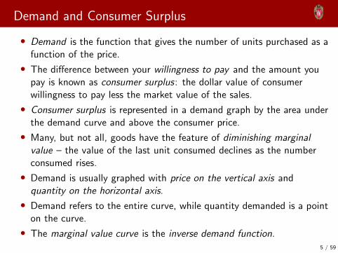
• Demand is the function that gives the number of units purchased as afunction of the price.
• The difference between your willingness to pay and the amount youpay is known as consumer surplus: the dollar value of consumerwillingness to pay less the market value of the sales.
• Consumer surplus is represented in a demand graph by the area underthe demand curve and above the consumer price.
• Many, but not all, goods have the feature of diminishing marginalvalue – the value of the last unit consumed declines as the numberconsumed rises.
• Demand is usually graphed with price on the vertical axis andquantity on the horizontal axis.
• Demand refers to the entire curve, while quantity demanded is a pointon the curve.
• The marginal value curve is the inverse demand function.5 / 59
Demand and Consumer Surplus (cont.)
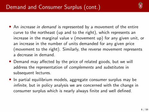
• An increase in demand is represented by a movement of the entirecurve to the northeast (up and to the right), which represents anincrease in the marginal value v (movement up) for any given unit, oran increase in the number of units demanded for any given price(movement to the right). Similarly, the reverse movement representsa decrease in demand.
• Demand may affected by the price of related goods, but we willaddress the representation of complements and substitutes insubsequent lectures.
• In partial equilibrium models, aggregate consumer surplus may beinfinite, but in policy analysis we are concerned with the change inconsumer surplus which is nearly always finite and well defined.
6 / 59
Supply and Profit
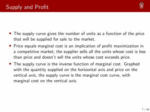
• The supply curve gives the number of units as a function of the pricethat will be supplied for sale to the market.
• Price equals marginal cost is an implication of profit maximization ina competitive market; the supplier sells all the units whose cost is lessthan price and doesn’t sell the units whose cost exceeds price.
• The supply curve is the inverse function of marginal cost. Graphedwith the quantity supplied on the horizontal axis and price on thevertical axis, the supply curve is the marginal cost curve, withmarginal cost on the vertical axis.
7 / 59

Supply and Profit (cont.)
• Profit is given by the difference of the price and marginal cost.
• An increase in supply refers to either more units available at a givenprice or a lower price for the supply of the same number of units.Thus, an increase in supply is graphically represented by a curve thatis lower or to the right, or both – that is, to the southeast. Adecrease in supply is the reverse case, a shift to the northwest.
• Anything that increases costs of production will tend to increasemarginal cost and thus reduce the supply.
8 / 59
Market Demand and Supply
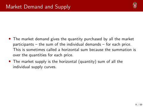
• The market demand gives the quantity purchased by all the marketparticipants – the sum of the individual demands – for each price.This is sometimes called a horizontal sum because the summation isover the quantities for each price.
• The market supply is the horizontal (quantity) sum of all theindividual supply curves.
9 / 59
Equilibrium
• The quantity supplied of a good or service exceeding the quantitydemanded is called a surplus.
• If the quantity demanded exceeds the quantity supplied, a shortageexists.
• The equilibrium price is the price in which the quantity suppliedequals the quantity demanded.
• The equilibrium of supply and demand maximizes the total gains fromtrade.
10 / 59

Changes in Demand and Supply
• An increase in the demand increases both the price and quantitytraded.
• A decrease in demand implies a fall in both the price and the quantitytraded.
• An increase in the supply decreases the price and increases thequantity traded.
• A decrease in the supply increases the price and decreases thequantity traded.
11 / 59
Changes in Demand and Supply (cont.)
• People react less to temporary changes than to permanent changes.People rationally continue to operate obsolete devices until theiruseful life is over, even when they wouldn’t buy an exact copy of thatdevice, an effect called hysteresis.
• Short-run and long-run effects represent a theme of economics, withthe major conclusion that substitution doesn’t occur instantaneously,which leads to predictable patterns of prices and quantities over time.
12 / 59

Elasticity
• The elasticity of demand is the percentage decrease in quantity thatresults from a small percentage increase in price, which is generallydenoted with the Greek letter epsilon, ε.
• The percentage change of total revenue resulting from a 1% changein price is one minus the elasticity of demand.
• An elasticity of demand that is less than one is defined as an inelasticdemand. In this case, increasing price increases total revenue.
• A price increase will decrease total revenue when the elasticity ofdemand is greater than one, which is defined as an elastic demand.
• The case of elasticity equal to one is called unitary elasticity, andtotal revenue is unchanged by a small price change.
13 / 59
Elasticity (cont)
• If demand takes the form x(p) = ap−ε, then demand has constantelasticity and the demand function is isoelastic with elasticity is equalto ε.
• The elasticity of supply is defined as the percentage increase inquantity supplied resulting from a small percentage increase in price.
• If supply takes the form s(p) = apη, then supply has constantelasticity, and the elasticity is equal to η.
14 / 59

Competitive Market Assumptions
• A market is typically competitive when there are many producers andconsumers.
• Assume are presently no taxes, and there is a stable equilibrium price.At this price, the elasticity of demand is ε and the elasticity of supplyis η.
• Assume that market demand and market supply curves are both linear.
15 / 59

Outline
• Recap
• Integrable functions
• Incidence and burden
• Global market for coal
• A model of carbon leakage
16 / 59
Calibrated Linear Demand and Supply
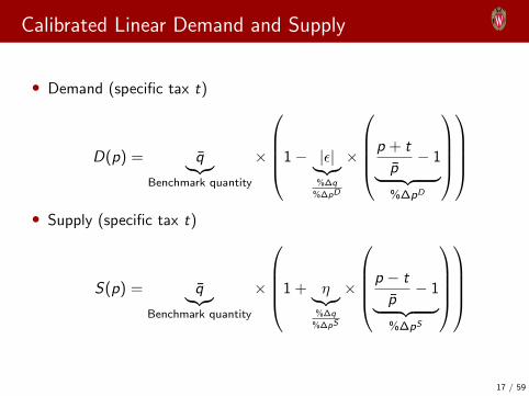
• Demand (specific tax t)
D(p) = q̄︸︷︷︸Benchmark quantity
×
1− |ε|︸︷︷︸%∆q
%∆pD
×
p + t
p̄− 1︸ ︷︷ ︸
%∆pD
• Supply (specific tax t)
S(p) = q̄︸︷︷︸Benchmark quantity
×
1 + η︸︷︷︸%∆q
%∆pS
×
p − t
p̄− 1︸ ︷︷ ︸
%∆pS
17 / 59

Calibrated Linear Demand and Supply
• Demand (ad-valorem tax τ)
D(p) = q̄︸︷︷︸Benchmark quantity
×
1− |ε|︸︷︷︸%∆q
%∆pD
×
p(1 + τ)
p̄− 1︸ ︷︷ ︸
%∆pD
• Supply (proportional tax ν)
S(p) = q̄︸︷︷︸Benchmark quantity
×
1 + η︸︷︷︸%∆q
%∆pS
×
p(1− ν)
p̄− 1︸ ︷︷ ︸
%∆pS
N.B. In this specification, τ is defined on a net basis while ν is defined ona gross basis.
18 / 59

Calibrated Isoelastic Demand and Supply
• Demand
D(p) = q̄
(p + t
p̄
)−ε
• Supply
S(p) = q̄
(p − t
p̄
)η
19 / 59
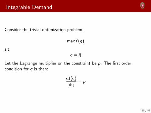
Integrable Demand
Consider the trivial optimization problem:
max f (q)
s.t.q = q̄
Let the Lagrange multiplier on the constraint be p. The first ordercondition for q is then:
df(q)
dq= p
20 / 59

Integrable Demand (cont.)
For what functional form f (q) is this first order condition equivalent to thefollowing?
A linear demand function
p = p̄
[1− 1
ε
(q
q̄− 1
)]An isoelastic demand function
p = p̄
(q
q̄
)−1/ε
21 / 59

Integrable Demand (cont.)
Representing p = g(q) implies
f (q) =
∫g(q)dq
In the case of the linear demand function we have
f (q) = p̄q
[1− 1
ε
(q
2q̄− 1
)]In the case of the isoelastic demand function we have
f (q) =p̄q
1− 1/ε
(q
q̄
)−1/ε
22 / 59

Outline
• Recap
• Integrable functions
• Incidence and burden
• Global market for coal
• A model of carbon leakage
23 / 59
Definitions of incidence.
Definition: tax incidence on consumers is the amount by which the buyerprice, PD , rises over the non-tax equilibrium price, P∗, ; the tax incidenceon producers is the amount by which the seller price, PS , falls below P∗.
The total tax wedge equals the sum of the tax incidence on the buyer andon the seller. The shares depend on the elasticities of demand and supply.The tax incidence is larger in the less elastic side of the market.
24 / 59

Incidence
If the gross of tax price increases from the reference price much more thanproducer price declines, then the consumer bears the burden of the tax. Ifthe gross of tax price increases much less than producer price declines,then the consumer bears the burden of the tax.
We can evaluate how the tax burden is allocated solely on the basis of theelasticities of supply and demand.
25 / 59

Incidence (cont.)
As expected, the producer price declines with the tax.
• Extreme case 1: supply is perfectly inelastic (η = 0) and the demandelasticity is not zero (ε < 0): the producer price declines one for onewith the tax.
• Extreme case 2: supply is elastic (η > 0) and demand is perfectlyinelastic (ε = 0): then the producer price is unaffected by the tax.
26 / 59

The new equilibrium (cont.)
The consumer price is given by:
p∗ + t = p0 +t
1− ε/η
The price impact on consumers likewise depends on demand and supplyelasticities. When demand is less elastic than supply, then the demandprice is more responsive to the tax increase. If supply is less elastic, thenthe demand price is unaffected.
27 / 59
Back of the envelope calculation of tax incidence
Changes in the demand price (PD) and the supply price (PS) are inverselyproportional to the ratio of the demand and supply elasticities:
∆PD
∆PS≈ η
ε
where:
η is the elasticity of supply,
ε is the elasticity of demand
28 / 59
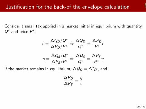
Justification for the back-of the envelope calculation
Consider a small tax applied in a market initial in equilibrium with quantityQ∗ and price P∗:
ε =∆QD/Q
∗
∆PD/P∗ ⇒∆QD
Q∗ =∆PD
P∗ ε
η =∆QS/Q
∗
∆PS/P∗ ⇒∆QS
Q∗ =∆PS
P∗ η
If the market remains in equilibrium, ∆QD = ∆QS , and
∆PD
∆PS=η
ε
29 / 59

Textbook exercise: tax incidence and burden
• The environment minister decides to levy an excise tax on coal salesat rate t.
• This means that if a seller receives p∗, the buyer pays p∗ + t.
• The demand price is therefore gross of tax and the producer price isnet of tax.
• When a tax is applied, the quantity transacted declines as theconsumer price (gross of tax) rises and the producer price (net of tax)declines.
30 / 59

A Textbook Exercise (cont.)
Given:
• Market equilibrium price equals $1 per unit.
• Quantity currently bought and sold equals 100 units.
• Price elasticity of supply equals 2.
• Price elasticity of demand equals 0.5.
31 / 59
The Problem
• A sales tax equal to 1 is applied to all transactions.
• Find the tax incidence.
• Find the resulting tax revenue.
• Find the change in consumer surplus.
• Find the change in producer surplus.
32 / 59

Solve the model... one equation in one unknown
D(p) = S(p)
or
100 (1− 0.5 (p + 1− 1)) = 100 (1 + 2(p − 1))
−0.5(p + 1− 1) = 2(p − 1)
2.5p = 2 ⇒ p∗ = 0.8
33 / 59

Solution:
• Supply price = p∗ = 0.8 (incidence = −0.2).
• Demand price = p∗ + t = 0.8 + 1 = 1.8 (incidence = +0.8).
• Equilibrium quantity: q∗ = 100× (1− 2× 0.2) = 60
• Tax revenue T = t × q∗ = 60
• Change in consumer suplus= −(60× 0.8 + 0.5× 40× 0.8) = −(48 + 16) = −64
• Change in producer surplus= −(60× 0.2 + 0.5× 40× 0.2 = −(12 + 4) = −16
34 / 59
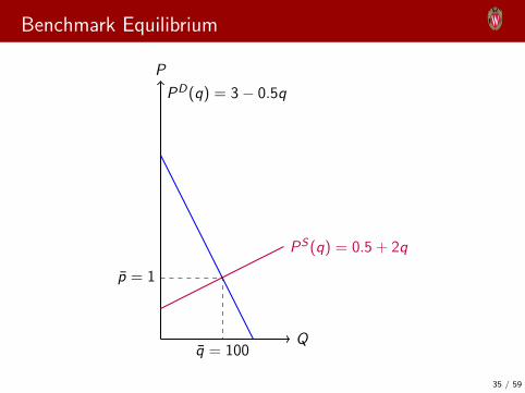
Benchmark Equilibrium
Q
P
PD(q) = 3− 0.5q
PS(q) = 0.5 + 2q
p̄ = 1
q̄ = 100
35 / 59
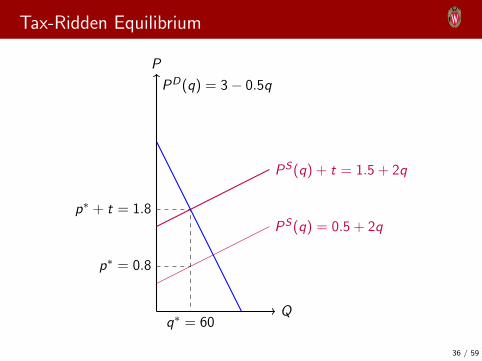
Tax-Ridden Equilibrium
Q
P
PD(q) = 3− 0.5q
PS(q) = 0.5 + 2q
PS(q) + t = 1.5 + 2q
p∗ + t = 1.8
q∗ = 60
p∗ = 0.8
36 / 59

Tax Revenue
Q
P
PD(q) = 3− 0.5q
PS(q) = 0.5 + 2q
PS(q) + t = 1.5 + 2q
p∗ = 0.8
p∗ + t = 1.8
q∗ = 60
37 / 59
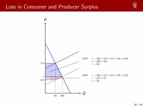
Loss in Consumer and Producer Surplus
Q
P
0.8
1
1.8
60 100
∆CS = −(60 × 0.8 + 0.5 × 40 × 0.8)= −(48 + 16)= −64
∆PS = −(60 × 0.2 + 0.5 × 40 × 0.2)= −(12 + 4)= −16
38 / 59

Outline
• Recap
• Integrable functions
• Incidence and burden
• Global market for coal
• A model of carbon leakage
39 / 59

Economic Models
Models play an important role in the formulation of trade policy. TheMarshallian market equilibrium model for competitive markets in whichsupply and demand are jointly determined along with price. We want tobegin with a graphical framework the implications of government policyinterventions in this model, interventions such as taxes, quotas, tariffs andsubsidies.
40 / 59

A Policy Issue
When Australia mitigates carbon emissions, this drives down the price ofcoal and increases incentives to coal exports. If coal exports increase, thiscan induced increased emissions in China.
The purpose of this computational exercise is to assess the globalenvironment effectiveness of subglobal policy measures. More to the point,to what extent does international trade vitiate the effectiveness of climatepolicy measures undertaken in a subset of regions.
41 / 59

Outline
• Recap
• Integrable functions
• Incidence and burden
• Global market for coal
• A model of carbon leakage
42 / 59
A Modeling Exercise
1 We find data on base year production, consumption and prices of coalin a collection of countries which collectively represent global coalsupply and demand.
2 Calibrate a model to these data.
3 Perform counterfactural analysis by applying excise taxes in a subsetof regions, corresponding to the coalition member states.
4 Assume that coal supply is price elastic (in the range of 1 to 2).
5 Assume that coal demand is price inelastic (in the range of 0.5).
6 Evaluate the global leakage rate:
` =% increase in coal use in non-coalition states
% decrease in coal use in coalition states
7 Does the leakage rate exceed 100%, as is claimed by some critical ofclimate policy?
8 Remember that The most interesting answer to any question ineconomics is: It depends.
43 / 59

A Modeling Exercise
1 We find data on base year production, consumption and prices of coalin a collection of countries which collectively represent global coalsupply and demand.
2 Calibrate a model to these data.
3 Perform counterfactural analysis by applying excise taxes in a subsetof regions, corresponding to the coalition member states.
4 Assume that coal supply is price elastic (in the range of 1 to 2).
5 Assume that coal demand is price inelastic (in the range of 0.5).
6 Evaluate the global leakage rate:
` =% increase in coal use in non-coalition states
% decrease in coal use in coalition states
7 Does the leakage rate exceed 100%, as is claimed by some critical ofclimate policy?
8 Remember that The most interesting answer to any question ineconomics is:
It depends.
43 / 59

A Modeling Exercise
1 We find data on base year production, consumption and prices of coalin a collection of countries which collectively represent global coalsupply and demand.
2 Calibrate a model to these data.
3 Perform counterfactural analysis by applying excise taxes in a subsetof regions, corresponding to the coalition member states.
4 Assume that coal supply is price elastic (in the range of 1 to 2).
5 Assume that coal demand is price inelastic (in the range of 0.5).
6 Evaluate the global leakage rate:
` =% increase in coal use in non-coalition states
% decrease in coal use in coalition states
7 Does the leakage rate exceed 100%, as is claimed by some critical ofclimate policy?
8 Remember that The most interesting answer to any question ineconomics is: It depends.
43 / 59

Coal Market Data: 1
44 / 59

Coal Market Data: 2
45 / 59

Coal Market Data: 3
46 / 59

Coal Market Data: 4
47 / 59

Coal Market Data: 5
48 / 59

Coal
BP Statistical Review of World Energy 2015 © BP p.l.c. 2015
49 / 59

BP Statistical Review of World Energy 2015 © BP p.l.c. 2015
Coal reserves-to-production (R/P) ratiosYears
2014 by region History
50 / 59
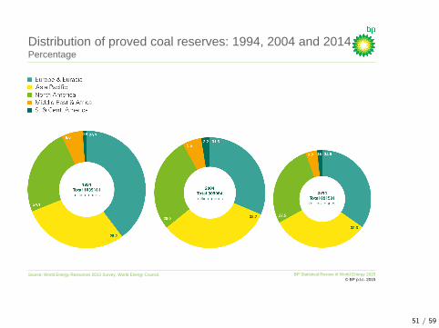
BP Statistical Review of World Energy 2015 © BP p.l.c. 2015
Source: World Energy Resources 2013 Survey, World Energy Council.
Distribution of proved coal reserves: 1994, 2004 and 2014Percentage
51 / 59
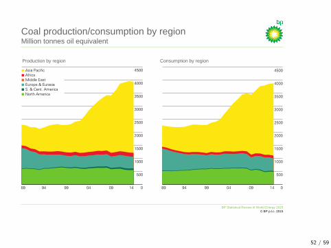
BP Statistical Review of World Energy 2015 © BP p.l.c. 2015
Coal production/consumption by regionMillion tonnes oil equivalent
Production by region Consumption by region
52 / 59

BP Statistical Review of World Energy 2015 © BP p.l.c. 2015
Coal consumption per capita 2014Tonnes oil equivalent
53 / 59

US Coal Use: Northern States
54 / 59
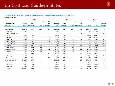
US Coal Use: Southern States
55 / 59
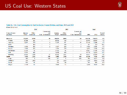
US Coal Use: Western States
56 / 59
Implementation
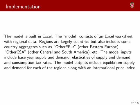
The model is built in Excel. The “model” consists of an Excel worksheetwith regional data. Regions are largely countries but also includes somecountry aggregates such as “OtherEEur” (other Eastern Europe),“OtherCSA” (other Central and South America), etc. The model inputsinclude base year supply and demand, elasticities of supply and demand,and consumption tax rates. The model outputs include equilibrium supplyand demand for each of the regions along with an international price index.
57 / 59
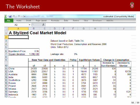
The Worksheet
58 / 59
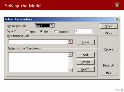
Solving the Model
59 / 59