Xiaosheng Bi, Jiayuan Zhuang * and Yumin Su

water

Article

Seakeeping Analysis of Planing Craft under LargeWave Height

Xiaosheng Bi, Jiayuan Zhuang * and Yumin Su

Science and Technology on Underwater Vehicle Laboratory, Harbin Engineering University, Harbin 150001,China; [email protected] (X.B.); [email protected] (Y.S.)* Correspondence: [email protected]

Received: 14 February 2020; Accepted: 31 March 2020; Published: 2 April 2020

Abstract: The purpose of this paper is to conduct a seakeeping analysis of planing craft under regularwave with large wave height. To obtain a reliable numerical method to simulate the sailing of planingcraft in waves, Reynolds-averaged Navier–Stokes (RANS) solver and overset method are adopted.The motion response and resistance of the planing craft USV01 in regular wave were numericalpredicted and compared with the corresponding seakeeping experimental tests. The results showthat the numerical method has high accuracy. For further study, a new planing craft whose nameis improved vessel is selected for simulation, the low steaming of the USV01 and improved vesselin regular wave with large wave height was simulated, and the seakeeping of the two vessels wasstudied. The analysis about the influence of wave length on the motion response and navigationconfigurations of the improved vessel under regular wave was carried out. Meanwhile, the influenceof speed on different navigation configurations of the improved vessel was also analyzed. Theimproved vessel can provide better seakeeping, and a reduction in the speed of the vessel will benefitits seakeeping, irrespective of its navigation configuration.

Keywords: planing craft; numerical method; seakeeping analysis; large wave height

1. Introduction

Planing craft have been widely used in various fields. The characteristic of the planing craft isthat the bottom of the vessel will come into contact with the free surface when sailing at high speed.Since the bottom is relatively flat, the water pressure at the bottom is increased because the bottom ofthe boat squeezes water forward [1].

For a better hydrodynamic performance, numerical prediction is becoming increasingly importantin the design of planing craft. The methods for predicting the resistance of planing craft includemodel test data, regression formulas, and semiempirical theory [2]. With the development of thecomputational fluid dynamics (CFD) method, the accuracy of numerical prediction in predictingthe hydrodynamic performance of planing craft under calm water and wave conditions has beenimproved. In 2017, Diez et al. [3] selected the DTMB 5415 model (US Navy Combatant) as the parenthull of the destroyer, and the hull of the destroyer was improved based on the CFD method. In 2018,Campana et al. [4] used the numerical method to optimize the hull of a high-speed catamaran, and areal ocean environment was also considered. Their results indicated that larger computational powerleads to an increase in computational efficiency and that the numerical method is becoming a necessarykey to optimizing hull design.

In 2001, Azcueta et al. [5] conducted deep research into the free motion simulation of planingcraft, based on the Comet, and the flow field around the hull were studied based on the k-ε turbulencemodel. Their results indicated that the numerical method can be adopted as an important complementto the study of the free surface flows around planing craft. In 2001, Caponnetto [6] conducted a

Water 2020, 12, 1020; doi:10.3390/w12041020 www.mdpi.com/journal/water

http://www.mdpi.com/journal/water

http://www.mdpi.com

http://dx.doi.org/10.3390/w12041020

http://www.mdpi.com/journal/water

https://www.mdpi.com/2073-4441/12/4/1020?type=check_update&version=2

Water 2020, 12, 1020 2 of 29

hydrodynamic analysis of a planing hull with an unknown center of gravity with Reynolds-averagedNavier–Stokes (RANS) solver. They also compared their results with Savitsky’s method. In 2015,Weymouth et al. [7] conducted an analysis on the sailing of a ship under head wave conditions basedon the unsteady RANS solver, and their work present accurate numerical results is uncertainties lessthan 2%. Their results indicate that the RANS solver has a better accuracy in simulating the sailing of avessel and that the solver is suitable for both high speed and head wave conditions.

In 2015, Sun et al. [8] researched the grid factor in the numerical calculation of planing craftresistance, based on the prismatic glider. The effect of different grid parameters on the accuracy ofthe numerical results was analyzed. With this grid scheme, the resistance of planing craft in variousnavigation states is calculated, and the numerical results present good accuracy. Their results are usefulfor the grid setup and boundary condition definition in this paper. In 2013, Su et al. [9] put forwarda numerical method to simulate the freedom motion of planing craft under head wave conditions,based on the six degrees of freedom (6-DOF) motion equation and volume of fluid (VOF) solver. Thecalculation results present a good agreement with the attitude of vessels under wave conditions. Theirresults show that the 6-DOF solver is suitable for simulating the motion of planing hull under headwave conditions. In 2017, De Marco et al. [10] conducted a seakeeping analysis of a stepped planingcraft. A hydrodynamic experiment of the single-step hull model, as a new systematic series, wascarried out, and the corresponding tests were based on numerical simulation, with an overset andmorphing grid. Their high-accuracy numerical results show that the overset mesh can improve theefficiency, while ensuring the accuracy of simulation, and the setting of the overset grid is of greatreferential significance to our work. In 2017, Dashtimanesh et al. [11] provided a numerical predictionof the performance of two-stepped planing craft. based on the mathematical model and the obtainedresults present the good accuracy compared with the test results. Their results indicate that the CFDmethod has become a fundamental support for the hydrodynamics study and design of planing craft,and it can be highly beneficial with respect to the cost and duration of hydrodynamic tests.

With the increasing demand for planing craft, the ability to sail in rough sea condition is necessary,and this requires an adequate seakeeping performance. However, traditional design of planing craftmakes it difficult to navigate safely. Due to the maturity of the numerical method, the complex motionproblems associated with viscous flow, the nonlinear problem, and the transient response problemcan all be directly solved by the numerical method. In 2000, Ikeda et al. [12] simulated the motion ofplaning craft under waves, and the porpoising oscillations and motion responses were numericallyforecasted. This means that the unsteady motion of vessels can also be numerically simulated. Thishas great significance for the study of the extremely high-speed navigation of planing craft. In 2003,Azcueta et al. [13] conducted an analysis on the speed performance of a power boat, based on thefree-surface RANS, and their method is suitable for predicting the severe responses of the vessel inwaves, making it possible to predict the nonlinear motion of planing craft in rough sea conditions.In 2014, Begovic et al. [14,15] conducted research on the responses of hull forms of a vessel in waves,and the response amplitudes in both regular and irregular waves were obtained and compared withthe corresponding test data. The Weibull distribution was adopted to analyze the motion response ofthe model in irregular waves, especially in relation to the acceleration of the center of gravity (CG).Irregular waves are closer to actual sea conditions, and the study of sailing in irregular waves is morereflective of actual sailing conditions. In 2016, Jiang et al. [16,17] conducted a study on the resistanceperformance of a planing trimaran with numerical and experimental methods. The CFD simulationswere based on 2-DOF motion equations, and high speed sailing of the vessel was simulated. Theresults were validated with a good accuracy by comparing them with the test data. Their experimentaldesign and setting is referential for our work, and their results indicate that numerical method can alsobe used to analyze the aerodynamic and hydrodynamic performance of trimaran.

In this paper, the STAR-CCM+ software (Germany) was adopted to simulate the sailing of asmall-scale planing craft under regular wave. In regular wave with large wave height, due to thelarge wave height and wave disturbance, planing craft need to maintain low-speed navigation. This

Water 2020, 12, 1020 3 of 29

paper will focus on the research of the motion response and navigation configuration of planing craftin regular wave with large wave height at a low speed. The RANS solver and overset grid wereadopted in the numerical simulation of the navigation of the vessel under head waves to obtain betteraccuracy, and validation was carried out by comparing the numerical results with the correspondingtest results. Additionally, a new planing craft with better seakeeping is selected for further analysis,the low steaming of both vessels in regular wave with large wave height was numerically simulatedand compared; and the influence of wave length and speed on the motion response and navigationconfiguration of the vessels is also analyzed.

Previous studies are mainly about the prediction of the motion response of planing craft, thispaper focus on the seakeeping and changes of navigation configuration of planing under the regularwave with large wave height. In 2019, we have carried out a research on the seakeeping analysis ofplaning craft [18], mainly focus on the optimization effect of hydrofoil. This paper aims to illustratea study on the navigation configuration of small planing craft under large wave height. And thenumerical methods used in the two papers are similar.

2. The Numerical Method

2.1. RANS Equation

To simulate the viscous flow field around a sailing ship is to solve the Navier–Stokes equation.In response to this problem, the RANS Equation is commonly used in engineering. In the actualsolving process, the time average value is used to replace the statistical average value, the momentumequations is as follows:

∂(ρui)

∂t+

∂∂xi

(ρuiu j) = −∂p∂xi

+∂∂x j

(µ∂ui∂x j− ρu′iu′ j) + Si (1)

Here ui and u j are the time mean of the velocity component, (i, j = 1, 2, 3), p is piezometric pressure

coefficient, ρ is fluid density, µ is coefficient of dynamic viscosity, ρu′i u′j is the Reynolds stress term, Sirepresents the generalized source term

Equation (1) and the continuity equation of incompressible fluid motion constitute the controlequations for solving the viscous flow field around the hull. The continuity equation is as follows:

∂ρ

∂t+∂(ρui)

∂xi= 0 (2)

In the RANS equation, the Reynolds stress term is introduced in addition to the progressiveequalization. In order to close the control equations, an appropriate turbulence model is introduced tocalculate the Reynolds stress term.

2.2. Turbulence Model

In this paper, the Shear Stress Transport turbulence (SST) model is used to seal the controlequations. The SST k–ωmodel [19] has been widely adopted in the solving of turbulence problems,especially the high Reynolds number flow problems, which is particularly suitable for the simulationof the high-speed navigation of planing craft. Similar to the k–ωmodel, the transport equation of k(turbulent kinetic energy) andω (dissipation rating) are presented as follows:

νt =a1k

max(a1ω; ΩF2)(3)

DρkDt

=∂∂x j

[(µ+ σkµt∂k∂x j

)] + τi j∂ui∂x j− β∗ρωk (4)

Water 2020, 12, 1020 4 of 29

(τi j = −ρui

′uj′

)(5)

DρωDt

=∂∂x j

[(µ+ σωµt∂ω∂x j

)] +γ

vtτi j∂ui∂x j− βρω2 + 2(1− F1)ρσω2

1ω∂k∂x j

∂ω∂x j

(6)

where Ω is the absolute value of the vorticity, ρ is fluid density.

F2 = tanh(arg2

2

)(7)

arg2= max(2

√k

0.09ωy;

500νy2ω

(8)

where y is the distance to the wall.The constants Φ are obtained from Φ1 and Φ2 .

Φ = F1Φ1 + (1− F1)Φ2 (9)

F1= tan h(arg 14

)(10)

arg1= min(max(

√k

0.09ωy;

500vy2ω

);4ρσω2kCDkωy2

(11)

CDkω = max(2ρσω21ω∂k∂x j

∂ω∂x j

; 10−20) (12)

The constants of Set Φ1 are Wilcox:

a1 = 0.31, σk1 = 0.85, σω1 = 0.5, β1 = 0.075,β∗ = 0.09,κ = 0.41,γ1 = β1/β∗ − σω1κ2/

√β∗

(13)

The constants of Set Φ2 are Jones–Launder:

a1 = 0.31, σk2 = 1, σω2 = 0.856, β2 = 0.0828,β∗ = 0.09,κ = 0.41,γ1 = β2/β∗ − σω2κ

2/√β∗

(14)

2.3. Boundary Conditions

The setting of the boundary conditions has a significant influence on solving physical problems offlow field. When the governing equation is given to solve different physical problems, the differentboundary value conditions are adopted. The boundary conditions are presented as follows:

Velocity inlet:The incoming boundary of the flow field, the boundary is usually set far from the ship. The

incoming velocity is given, the pressure is obtained by using reconstructed gradient interpolation.

v = (U, 0, 0) (15)

dpdn

= 0 (16)

The estimation formula of k andω are:

k =32(IkU)2 (17)

ω = ρkµ(µt

µ)−1

(18)

Water 2020, 12, 1020 5 of 29

α =

1 z ≤ 00 z > 0

(19)

Ik is turbulence intensity, µt/µ is turbulent viscosity ratio, α is volume fraction.Pressure outlet:The outlet of the flow field in the computation domain, it is set far behind the stern. The variables

of outlet boundary are generally unknown, but the boundary is usually far away from the hull, thephysical variables change little. Except for the pressure, the normal gradient of other physical variablesis zero:

∂u∂n

= 0,∂k∂n

= 0,∂ω∂n

= 0,∂α∂n

= 0 (20)

Symmetry plane:To reduce the total number of grids, only half computation domain is typically built, the symmetry

plane has no physical meaning. The normal velocity of the boundary is zero, the gradient of thephysical quantity of the flow is zero.

un = n · v = 0 (21)

∂u∂n

= 0,∂k∂n

= 0,∂ω∂n

= 0,∂α∂n

= 0 (22)

Wall condition:In the computation domain, only the hull needs wall conditions. The wall surface of the hull is

non-slippable:v = (0, 0, 0) (23)

dpdn

= 0 (24)

2.4. Wall y+

In the numerical simulation of turbulence, especially with respect to the high Reynolds numberproblems, the hull is regarded as a non-slip wall, and because of the viscous damping of the wall, thevelocity gradient near the hull is very large. In the numerical method, the wall function is used for thenear wall treatment as a hybrid approach. In 2005, Wang [20] conducted research on the turbulenceproblem, indicating that the y+ value near the hull should be controlled between 30 and 300. The wally+ value is dimensionless quantity, and the formula for calculating the y+ value is as follows:

y+ =yυ

√√12

U2 0.074

Re15L

(25)

Here y is the distance from the wall to the boundary layer grid; U is the speed; v is the fluidviscosity coefficient; Re is the Reynolds number.

In the numerical simulation, the prism layer grid is generated to replace boundary layer. However,due to the intense motion of the planing craft, the waterline length will be sharply reduced as well.A low y+ value will greatly affect the accuracy, the value of y+ should be larger.

2.5. Volume of Fluid Method

In the numerical simulations of the sailing of vessel, the flow field is complex, tracking the freesurface with a high accuracy method will ensure the accuracy of numerical simulation. To solve thisproblem, in 1981, Nichols and Hirt [21] proposed the volume of fluid method (VOF). The VOF methodis to obtain and track the function F, which is defined as the volume ratio of different fluid occupancy

Water 2020, 12, 1020 6 of 29

in the grid. If the value of this function on each grid is obtained, the motion interface of the two phasesof the flow will be tracked. The function F is defined as follows [22]:

∂F∂t

+ u∂F∂x

+ v∂F∂y

+ w∂F∂z

= 0 (26)

Here u, v, w are the velocity components.

2.6. Overset Method

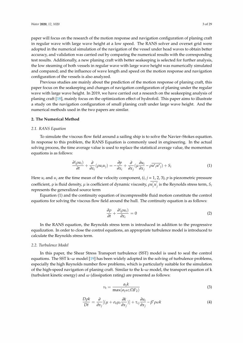
Overset grid is the method of region segmentation and grid combination, which consists ofbackground and overset region. The overset method consists of two parts: (1) Divided grid cells in thewhole flow field area into effective cells and invalid cells by hole cutting. Effective cell refers to the gridcell which participates in solving discrete governing equations, the grid cells that do not participatein computation are invalid cells. (2) Find the contributor cell, which configures the correspondingcontributor cell for the recipient cell. The receiver cell layer is formed along the boundary of the oversetregion, and it is this layer of receiver cell layer that divides the background grid into effective cellregion and invalid cell region. The overset region and the background region are closely coupled, andthe governing equation is solved simultaneously in the effective cells of the two regions. The oversetgrid around the hull is presented in Figure 1.

Water 2020, 12, x 6 of 30

2.5. Volume of Fluid Method

In the numerical simulations of the sailing of vessel, the flow field is complex, tracking the free

surface with a high accuracy method will ensure the accuracy of numerical simulation. To solve this

problem, in 1981, Nichols and Hirt [21] proposed the volume of fluid method (VOF). The VOF

method is to obtain and track the function F, which is defined as the volume ratio of different fluid

occupancy in the grid. If the value of this function on each grid is obtained, the motion interface of

the two phases of the flow will be tracked. The function F is defined as follows [22]:

0F F F F

u v wt x y z

(26)

Here u, v, w are the velocity components.

2.6. Overset Method

Overset grid is the method of region segmentation and grid combination, which consists of

background and overset region. The overset method consists of two parts: (1) Divided grid cells in

the whole flow field area into effective cells and invalid cells by hole cutting. Effective cell refers to

the grid cell which participates in solving discrete governing equations, the grid cells that do not

participate in computation are invalid cells. (2) Find the contributor cell, which configures the

corresponding contributor cell for the recipient cell. The receiver cell layer is formed along the

boundary of the overset region, and it is this layer of receiver cell layer that divides the background

grid into effective cell region and invalid cell region. The overset region and the background region

are closely coupled, and the governing equation is solved simultaneously in the effective cells of the

two regions. The overset grid around the hull is presented in Figure 1.

Figure 1. Background grid and overset grid.

3. Towing Tank Experiments

To validate the accuracy of the numerical method, a planing craft model (USV01) is selected as

the study object. The seakeeping tests of USV01 were carried out in 2011 by Hailong Shen and

colleagues [18]. The hull model and the specific parameters of the model are presented in Figure 2

and Table 1.

Table 1. Parameters of the model of USV01.

Main feature Symbol Value

Model scale k 1:4

Length overall L 2.75 m

Beam overall B 0.78 m

Mouded depth h 0.325 m

Displacement Δ 125.4 kg

Draft d 0.1325 m

Longitudinal position of the centre of gravity 𝐿 1.048 m

Rotational inertia J 58.6 (kg∙m2)

Figure 1. Background grid and overset grid.

3. Towing Tank Experiments

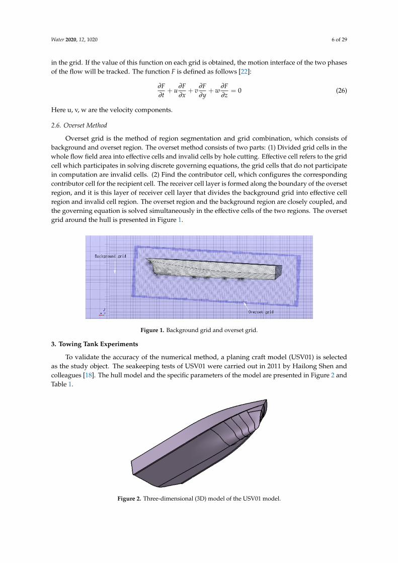
To validate the accuracy of the numerical method, a planing craft model (USV01) is selectedas the study object. The seakeeping tests of USV01 were carried out in 2011 by Hailong Shen andcolleagues [18]. The hull model and the specific parameters of the model are presented in Figure 2 andTable 1.

Water 2020, 12, x 7 of 30

Deadrise angle β 18 deg

Figure 2. Three‐dimensional (3D) model of the USV01 model.

The setup of test is presented in Figure 3. All the experimental installations were installed under

the carriage platform, and the guide rods are inserted into the guide plates, which were set at the bow

and stern to ensure stability in the drag. In this way, the yaw and roll motions are prevented, and the

heave and pitch motions of the model are free. The resistance is measured by a dynamometer in the

front of the model, the pitch angle is measured by a gyroscope, which is set at the center of gravity,

the heave is measured by the cable‐extension displacement sensor, which is set on the above model,

and the acceleration of the CG and bow of the model are measured by two acceleration sensors, which

are set at the center of gravity and 0.275 m from bow. A snapshot of the model is presented in Figure

4.

Figure 3. Experimental setup.

Figure 2. Three-dimensional (3D) model of the USV01 model.

Water 2020, 12, 1020 7 of 29

Table 1. Parameters of the model of USV01.


Model scale k 1:4Length overall L 2.75 mBeam overall B 0.78 m

Mouded depth h 0.325 mDisplacement ∆ 125.4 kg

Draft d 0.1325 mLongitudinal position of the centre of gravity LCG 1.048 m

Rotational inertia J 58.6 (kg·m2)Deadrise angle β 18 deg

The setup of test is presented in Figure 3. All the experimental installations were installed underthe carriage platform, and the guide rods are inserted into the guide plates, which were set at the bowand stern to ensure stability in the drag. In this way, the yaw and roll motions are prevented, and theheave and pitch motions of the model are free. The resistance is measured by a dynamometer in thefront of the model, the pitch angle is measured by a gyroscope, which is set at the center of gravity, theheave is measured by the cable-extension displacement sensor, which is set on the above model, andthe acceleration of the CG and bow of the model are measured by two acceleration sensors, which areset at the center of gravity and 0.275 m from bow. A snapshot of the model is presented in Figure 4.

Water 2020, 12, x 7 of 30


Figure 2. Three‐dimensional (3D) model of the USV01 model.

The setup of test is presented in Figure 3. All the experimental installations were installed under

the carriage platform, and the guide rods are inserted into the guide plates, which were set at the bow

and stern to ensure stability in the drag. In this way, the yaw and roll motions are prevented, and the

heave and pitch motions of the model are free. The resistance is measured by a dynamometer in the

front of the model, the pitch angle is measured by a gyroscope, which is set at the center of gravity,

the heave is measured by the cable‐extension displacement sensor, which is set on the above model,

and the acceleration of the CG and bow of the model are measured by two acceleration sensors, which

are set at the center of gravity and 0.275 m from bow. A snapshot of the model is presented in Figure

4.

Figure 3. Experimental setup. Figure 3. Experimental setup.

Water 2020, 12, 1020 8 of 29

Water 2020, 12, x 8 of 30

Figure 4. Snapshot of the model.

In the regular wave test, the towed velocity (U) was 6 m/s (Fn = 1.16), the wave height is 0.21 m,

and the wave length ranged from 1.5 L to 5 L. The regular wave test matrix is presented in Table 2,

where the wave length is λ, the wave height is H, and the encounter frequency is ω. The motion

parameters of the model were read when it crossed ten wave lengths in waves.

Table 2. Regular wave test matrix of the seakeeping test.

No. U (m/s) Fn H (m) λ/L λ(m) 𝛚 (rad/s) H/λ

1 6 1.16 0.21 1.5 4.125 13.031 0.051

2 6 1.16 0.21 2.25 6.1875 9.261 0.034

3 6 1.16 0.21 3 8.25 7.301 0.025

4 6 1.16 0.21 3.5 9.625 6.446 0.022

5 6 1.16 0.21 4 11 5.787 0.019

6 6 1.16 0.21 5 13.75 4.816 0.015

Under the same speed and wave height, based on the curves of the model’s motion, the peak–

peak values of the motion response and the average resistance of the model in different conditions

were obtained.

4. Numerical Simulation Validation

4.1. Computational Domains

For a better accuracy, the boundaries of the calculation domain were set far enough away to

reduce the reflection of waves, and the entire computational domain should be no less than five times

the wave length in the navigation direction. To improve the computing efficiency, only half of the

model was built for the simulation. The definition of the boundary conditions and the size of domains

are illustrated in Figure 5 and Table 3, respectively.

The point at the bottom of the stern is set as the origin. The distance between each boundary and

the origin are presented in Table 3, and all the distances are dimensionalized in terms of the overall

length of the model.

Figure 4. Snapshot of the model.

In the regular wave test, the towed velocity (U) was 6 m/s (Fn = 1.16), the wave height is 0.21 m,and the wave length ranged from 1.5 L to 5 L. The regular wave test matrix is presented in Table 2,where the wave length is λ, the wave height is H, and the encounter frequency is ω. The motionparameters of the model were read when it crossed ten wave lengths in waves.

Table 2. Regular wave test matrix of the seakeeping test.

No. U (m/s) Fn H (m) λ/L λ(m) ω (rad/s) H/λ

1 6 1.16 0.21 1.5 4.125 13.031 0.0512 6 1.16 0.21 2.25 6.1875 9.261 0.0343 6 1.16 0.21 3 8.25 7.301 0.0254 6 1.16 0.21 3.5 9.625 6.446 0.0225 6 1.16 0.21 4 11 5.787 0.0196 6 1.16 0.21 5 13.75 4.816 0.015

Under the same speed and wave height, based on the curves of the model’s motion, thepeak–peak values of the motion response and the average resistance of the model in different conditionswere obtained.

4. Numerical Simulation Validation

4.1. Computational Domains

For a better accuracy, the boundaries of the calculation domain were set far enough away toreduce the reflection of waves, and the entire computational domain should be no less than five timesthe wave length in the navigation direction. To improve the computing efficiency, only half of themodel was built for the simulation. The definition of the boundary conditions and the size of domainsare illustrated in Figure 5 and Table 3, respectively.

The point at the bottom of the stern is set as the origin. The distance between each boundary andthe origin are presented in Table 3, and all the distances are dimensionalized in terms of the overalllength of the model.

Water 2020, 12, 1020 9 of 29

Water 2020, 12, x 9 of 30

Table 3. Sizes of the computational domains.

Boundary Distance Boundary conditions

Inlet 2.5 L Velocity inlet

Outlet 4 L Pressure outlet

Top 2 L Velocity inlet

Bottom 1 L Velocity inlet

Side 1.5 L Symmetry plane

Inlet of overset region 1.25 L

Overset grid

Outlet of overset region 0.25 L

Top of overset region 0.25 L

Bottom of overset region 0.25 L

Side of overset region 0.3 L

Figure 5. The size of the calculation domains.

The definitions of boundary conditions in the domain are presented as follow: in the background

region, the inlet, top and bottom are defined as the velocity inlet; the outlet is defined as the pressure

outlet; and the sym and side are defined as the symmetry plane. In the overset region, all the

boundaries of the region are defined as the overset grid, and the surface of the hull is defined as the

nonslip wall. The definition of the boundary conditions and the setting of the calculation domains

are illustrated in Figure 6.

Figure 5. The size of the calculation domains.

Table 3. Sizes of the computational domains.

Boundary Distance Boundary Conditions

Inlet 2.5 L Velocity inletOutlet 4 L Pressure outlet

Top 2 L Velocity inletBottom 1 L Velocity inlet

Side 1.5 L Symmetry planeInlet of overset region 1.25 L

Overset gridOutlet of overset region 0.25 L

Top of overset region 0.25 LBottom of overset region 0.25 L

Side of overset region 0.3 L

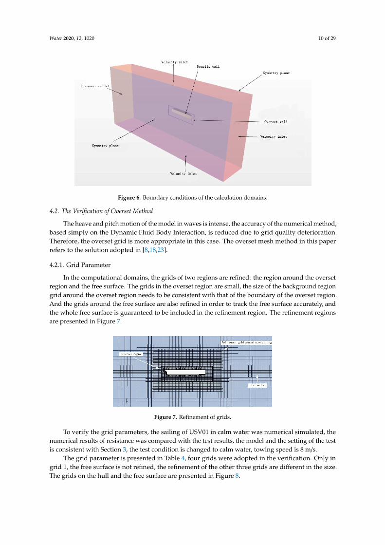
The definitions of boundary conditions in the domain are presented as follow: in the backgroundregion, the inlet, top and bottom are defined as the velocity inlet; the outlet is defined as the pressureoutlet; and the sym and side are defined as the symmetry plane. In the overset region, all the boundariesof the region are defined as the overset grid, and the surface of the hull is defined as the nonslip wall.The definition of the boundary conditions and the setting of the calculation domains are illustrated inFigure 6.

Water 2020, 12, 1020 10 of 29Water 2020, 12, x 10 of 30

Figure 6. Boundary conditions of the calculation domains.

4.2. The Verification of Overset Method

The heave and pitch motion of the model in waves is intense, the accuracy of the numerical

method, based simply on the Dynamic Fluid Body Interaction, is reduced due to grid quality

deterioration. Therefore, the overset grid is more appropriate in this case. The overset mesh method

in this paper refers to the solution adopted in [8,18,23].

4.2.1. Grid Parameter

In the computational domains, the grids of two regions are refined: the region around the overset

region and the free surface. The grids in the overset region are small, the size of the background

region grid around the overset region needs to be consistent with that of the boundary of the overset

region. And the grids around the free surface are also refined in order to track the free surface

accurately, and the whole free surface is guaranteed to be included in the refinement region. The

refinement regions are presented in Figure 7.

Figure 7. Refinement of grids.

To verify the grid parameters, the sailing of USV01 in calm water was numerical simulated, the

numerical results of resistance was compared with the test results, the model and the setting of the

test is consistent with section 3, the test condition is changed to calm water, towing speed is 8 m/s.

The grid parameter is presented in Table 4, four grids were adopted in the verification. Only in

grid 1, the free surface is not refined, the refinement of the other three grids are different in the size.

The grids on the hull and the free surface are presented in Figure 8.



The heave and pitch motion of the model in waves is intense, the accuracy of the numerical method,based simply on the Dynamic Fluid Body Interaction, is reduced due to grid quality deterioration.Therefore, the overset grid is more appropriate in this case. The overset mesh method in this paperrefers to the solution adopted in [8,18,23].


In the computational domains, the grids of two regions are refined: the region around the oversetregion and the free surface. The grids in the overset region are small, the size of the background regiongrid around the overset region needs to be consistent with that of the boundary of the overset region.And the grids around the free surface are also refined in order to track the free surface accurately, andthe whole free surface is guaranteed to be included in the refinement region. The refinement regionsare presented in Figure 7.

Water 2020, 12, x 10 of 30



The heave and pitch motion of the model in waves is intense, the accuracy of the numerical

method, based simply on the Dynamic Fluid Body Interaction, is reduced due to grid quality

deterioration. Therefore, the overset grid is more appropriate in this case. The overset mesh method

in this paper refers to the solution adopted in [8,18,23].


In the computational domains, the grids of two regions are refined: the region around the overset

region and the free surface. The grids in the overset region are small, the size of the background

region grid around the overset region needs to be consistent with that of the boundary of the overset

region. And the grids around the free surface are also refined in order to track the free surface

accurately, and the whole free surface is guaranteed to be included in the refinement region. The

refinement regions are presented in Figure 7.


To verify the grid parameters, the sailing of USV01 in calm water was numerical simulated, the

numerical results of resistance was compared with the test results, the model and the setting of the

test is consistent with section 3, the test condition is changed to calm water, towing speed is 8 m/s.

The grid parameter is presented in Table 4, four grids were adopted in the verification. Only in

grid 1, the free surface is not refined, the refinement of the other three grids are different in the size.

The grids on the hull and the free surface are presented in Figure 8.


To verify the grid parameters, the sailing of USV01 in calm water was numerical simulated, thenumerical results of resistance was compared with the test results, the model and the setting of the testis consistent with Section 3, the test condition is changed to calm water, towing speed is 8 m/s.

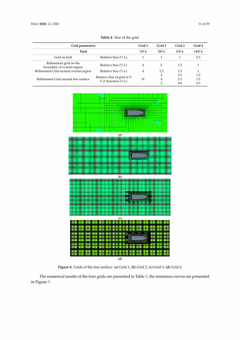
The grid parameter is presented in Table 4, four grids were adopted in the verification. Only ingrid 1, the free surface is not refined, the refinement of the other three grids are different in the size.The grids on the hull and the free surface are presented in Figure 8.

Water 2020, 12, 1020 11 of 29

Table 4. Size of the grid.

Grid parameters Grid 1 Grid 2 Grid 3 Grid 4

Total 150 k 280 k 650 k 1400 k

Grid on hull Relative Size (% L) 1 1 1 0.5

Refinement grid on theboundary of overset region Relative Size (% L) 4 2. 1.5 1

Refinement Grid around overset region Relative Size (% L) 4 2.5 1.5 1

Refinement Grid around free surface Relative Size of grid in XY Z direction (% L) N

442

2.52.50.8

1.51.50.5

Water 2020, 12, x 11 of 30

Table 4. Size of the grid.

Grid parameters Grid 1 Grid 2 Grid 3 Grid 4

Total 150 k 280 k 650 k 1400 k

Grid on hull Relative Size (% L) 1 1 1 0.5

Refinement

grid on the

boundary of

overset region

Relative Size (% L) 4 2. 1.5 1

Refinement

Grid around

overset region

Relative Size (% L) 4 2.5 1.5 1

Refinement

Grid around

free surface

Relative Size of

grid in X Y Z

direction (% L)

N

4

4

2

2.5

2.5

0.8

1.5

1.5

0.5

(a)

(b)

(c)

(d)

Figure 8. Grids of the free surface: (a) Grid 1, (b) Grid 2, (c) Grid 3, (d) Grid 4.

Figure 8. Grids of the free surface: (a) Grid 1, (b) Grid 2, (c) Grid 3, (d) Grid 4.

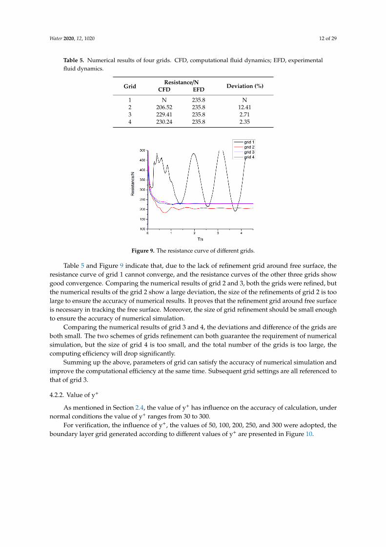
The numerical results of the four grids are presented in Table 5, the resistance curves are presentedin Figure 9.

Water 2020, 12, 1020 12 of 29

Table 5. Numerical results of four grids. CFD, computational fluid dynamics; EFD, experimentalfluid dynamics.

GridResistance/N

Deviation (%)CFD EFD

1 N 235.8 N2 206.52 235.8 12.413 229.41 235.8 2.714 230.24 235.8 2.35

Water 2020, 12, x 12 of 30

The numerical results of the four grids are presented in Table 5, the resistance curves are

presented in Figure 9.

Table 5. Numerical results of four grids. CFD, computational fluid dynamics; EFD, experimental

fluid dynamics.

Grid Resistance/N

Deviation (%) CFD EFD

1 N 235.8 N

2 206.52 235.8 12.41

3 229.41 235.8 2.71

4 230.24 235.8 2.35

Figure 9. The resistance curve of different grids.

Table 5 and Figure 9 indicate that, due to the lack of refinement grid around free surface, the

resistance curve of grid 1 cannot converge, and the resistance curves of the other three grids show

good convergence. Comparing the numerical results of grid 2 and 3, both the grids were refined, but

the numerical results of the grid 2 show a large deviation, the size of the refinements of grid 2 is too

large to ensure the accuracy of numerical results. It proves that the refinement grid around free

surface is necessary in tracking the free surface. Moreover, the size of grid refinement should be small

enough to ensure the accuracy of numerical simulation.

Comparing the numerical results of grid 3 and 4, the deviations and difference of the grids are

both small. The two schemes of grids refinement can both guarantee the requirement of numerical

simulation, but the size of grid 4 is too small, and the total number of the grids is too large, the

computing efficiency will drop significantly.

Summing up the above, parameters of grid can satisfy the accuracy of numerical simulation and

improve the computational efficiency at the same time. Subsequent grid settings are all referenced to

that of grid 3.

4.2.2. Value of y+

As mentioned in section 2.4, the value of y+ has influence on the accuracy of calculation, under

normal conditions the value of y+ ranges from 30 to 300.

For verification, the influence of y+, the values of 50, 100, 200, 250, and 300 were adopted, the

boundary layer grid generated according to different values of y+ are presented in Figure 10.

Figure 9. The resistance curve of different grids.

Table 5 and Figure 9 indicate that, due to the lack of refinement grid around free surface, theresistance curve of grid 1 cannot converge, and the resistance curves of the other three grids showgood convergence. Comparing the numerical results of grid 2 and 3, both the grids were refined, butthe numerical results of the grid 2 show a large deviation, the size of the refinements of grid 2 is toolarge to ensure the accuracy of numerical results. It proves that the refinement grid around free surfaceis necessary in tracking the free surface. Moreover, the size of grid refinement should be small enoughto ensure the accuracy of numerical simulation.

Comparing the numerical results of grid 3 and 4, the deviations and difference of the grids areboth small. The two schemes of grids refinement can both guarantee the requirement of numericalsimulation, but the size of grid 4 is too small, and the total number of the grids is too large, thecomputing efficiency will drop significantly.

Summing up the above, parameters of grid can satisfy the accuracy of numerical simulation andimprove the computational efficiency at the same time. Subsequent grid settings are all referenced tothat of grid 3.

4.2.2. Value of y+

As mentioned in Section 2.4, the value of y+ has influence on the accuracy of calculation, undernormal conditions the value of y+ ranges from 30 to 300.

For verification, the influence of y+, the values of 50, 100, 200, 250, and 300 were adopted, theboundary layer grid generated according to different values of y+ are presented in Figure 10.


(a)

(b)

(c)

(d)

(e)

Figure 10. Boundary layer grid: (a) y+ = 50, (b) y+ = 100, (c) y+ = 200, (d) y+ = 250, (e) y+ = 300. Figure 10. Boundary layer grid: (a) y+ = 50, (b) y+ = 100, (c) y+ = 200, (d) y+ = 250, (e) y+ = 300.

Water 2020, 12, 1020 14 of 29

The Figure 10 indicates that the trim motion of the planing craft leads to a great change of thewaterline of the vessel. The decrease of the waterline length makes the y+ value of hull less than thetheoretical value during the sailing.

The numerical results and the resistance curves of different y+ are presented in Table 6 andFigure 11, respectively.

Table 6. Numerical results of different y+.

y+ Resistance/NDeviation (%)CFD EFD

50 223.06 235.8 5.4100 220.82 235.8 6.35200 221.78 235.8 5.95250 229.41 235.8 2.71300 228.56 235.8 3.14

Water 2020, 12, x 14 of 30

The Figure 10 indicates that the trim motion of the planing craft leads to a great change of the

waterline of the vessel. The decrease of the waterline length makes the y+ value of hull less than the

theoretical value during the sailing.

The numerical results and the resistance curves of different y+ are presented in Table 6 and

Figure 11, respectively.

Table 6. Numerical results of different y+.

y+ Resistance/N


50 223.06 235.8 5.4

100 220.82 235.8 6.35

200 221.78 235.8 5.95

250 229.41 235.8 2.71

300 228.56 235.8 3.14

Figure 11. The resistance curve of different y+ s.

The Table 6 and Figure 11 indicate that resistance curves corresponding different y+ have similar

convergence. The deviations of different values of y+ are all less than 10%, but the deviation which y+

= 250 is the smallest. Due to the intense motion of the planing craft, the waterline length sharply

reduces. A low y+ value greatly affect the accuracy. In subsequent numerical simulations, the y+ value

was set at 250.

4.2.3. Time Step of Iteration

The ∆t (time step) of iteration should be set at the value which allows the physical field to move

no less than the distance of the minimum free surface mesh in each iteration, thus improving the

calculation efficiency, with the aim of ensuring accuracy.

To verify the value of ∆t, four values: 0.001 s, 0.002 s, 0.006 s, 0.01 s, 0.02 s were adopted and the

numerical results corresponding to different values were compared in Table 7 and the resistance

curves of different y+ are presented Figure 12.

Table 7. Numerical results of different ∆t (time steps).

∆t (s) Resistance/N


0.001 228.84 235.8 3.11

0.002 229.41 235.8 2.71

0.006 209.72 235.8 11.06

0.01 200.82 235.8 14.83

0.02 180.66 235.8 23.38

Figure 11. The resistance curve of different y+ s.

The Table 6 and Figure 11 indicate that resistance curves corresponding different y+ have similarconvergence. The deviations of different values of y+ are all less than 10%, but the deviation whichy+ = 250 is the smallest. Due to the intense motion of the planing craft, the waterline length sharplyreduces. A low y+ value greatly affect the accuracy. In subsequent numerical simulations, the y+ valuewas set at 250.

4.2.3. Time Step of Iteration

The ∆t (time step) of iteration should be set at the value which allows the physical field to moveno less than the distance of the minimum free surface mesh in each iteration, thus improving thecalculation efficiency, with the aim of ensuring accuracy.

To verify the value of ∆t, four values: 0.001 s, 0.002 s, 0.006 s, 0.01 s, 0.02 s were adopted and thenumerical results corresponding to different values were compared in Table 7 and the resistance curvesof different y+ are presented Figure 12.

Table 7. Numerical results of different ∆t (time steps).

∆t (s)Resistance/N

Deviation (%)CFD EFD

0.001 228.84 235.8 3.110.002 229.41 235.8 2.710.006 209.72 235.8 11.060.01 200.82 235.8 14.830.02 180.66 235.8 23.38


Figure 12. The resistance curve of different ∆t.

The comparison between results of different values of ∆t indicate that the convergence trends of

the five resistance curves are consistent, but different values will affect the accuracy of numerical

results. The deviations of the results become larger with the increasing of ∆t, this indicates a short

time interval between two iterations will benefit the accuracy of the numerical results. But a too small

value of ∆t can lead to a waste of computational efficiency. The results of ∆t = 0.001 s and 0.002 s are

almost the same and the accuracy is high, ∆t = 0.002 s is adopted for its better accuracy and

computational efficiency.

Summing up the above, the influence of the grid parameter, value of y+, and the time step of

iteration on the accuracy and computational efficiency are verified. The results show that the

numerical method has good convergence and high accuracy in simulating of the sailing of USV01 in

calm water. Based on the overset method which has been verified, the numerical simulation

validation for the seakeeping test of USV01 will be carried out.

4.3. Validation of Numerical Method

On the basis of the verification of overset method, the grid parameters refer to grid 3, the value

of y+ is set at 250, the ∆t is set at 0.002 s. In this way both the accuracy and computational efficiency

are guaranteed.

In the numerical simulation of seakeeping tests, the setting of calculation domains, grid

parameters, and ∆t are referenced to the section 4.1 and 4.2, meanwhile, in the wave conditions the

flow field of the free surface is more complicated, the refinement region around the free surface needs

to contain the entire wave surface and the vertical refinement grid should be not less than 10 layers.

When the motion of the model in regular wave tends to stabilize and sails at least five wave lengths,

the response amplitude operators of the model were obtained. The calculation grids of the numerical

simulations of seakeeping tests are presented in Figure 13.

Figure 12. The resistance curve of different ∆t.

The comparison between results of different values of ∆t indicate that the convergence trends ofthe five resistance curves are consistent, but different values will affect the accuracy of numerical results.The deviations of the results become larger with the increasing of ∆t, this indicates a short time intervalbetween two iterations will benefit the accuracy of the numerical results. But a too small value of ∆t canlead to a waste of computational efficiency. The results of ∆t = 0.001 s and 0.002 s are almost the sameand the accuracy is high, ∆t = 0.002 s is adopted for its better accuracy and computational efficiency.

Summing up the above, the influence of the grid parameter, value of y+, and the time step ofiteration on the accuracy and computational efficiency are verified. The results show that the numericalmethod has good convergence and high accuracy in simulating of the sailing of USV01 in calm water.Based on the overset method which has been verified, the numerical simulation validation for theseakeeping test of USV01 will be carried out.

4.3. Validation of Numerical Method

On the basis of the verification of overset method, the grid parameters refer to grid 3, the valueof y+ is set at 250, the ∆t is set at 0.002 s. In this way both the accuracy and computational efficiencyare guaranteed.

In the numerical simulation of seakeeping tests, the setting of calculation domains, grid parameters,and ∆t are referenced to the Sections 4.1 and 4.2, meanwhile, in the wave conditions the flow field ofthe free surface is more complicated, the refinement region around the free surface needs to containthe entire wave surface and the vertical refinement grid should be not less than 10 layers. When themotion of the model in regular wave tends to stabilize and sails at least five wave lengths, the responseamplitude operators of the model were obtained. The calculation grids of the numerical simulations ofseakeeping tests are presented in Figure 13.

Water 2020, 12, 1020 16 of 29

Water 2020, 12, x 16 of 30

(a)

(b)

(c)

(d)

(e)

Figure 13. Calculation grids: (a) Domain grids; (b) Medium‐profile local grids; (c) Surface grid on the

hull; (d) Grid near free surface; (e) Free surface of regular wave. Figure 13. Calculation grids: (a) Domain grids; (b) Medium-profile local grids; (c) Surface grid on thehull; (d) Grid near free surface; (e) Free surface of regular wave.

Water 2020, 12, 1020 17 of 29

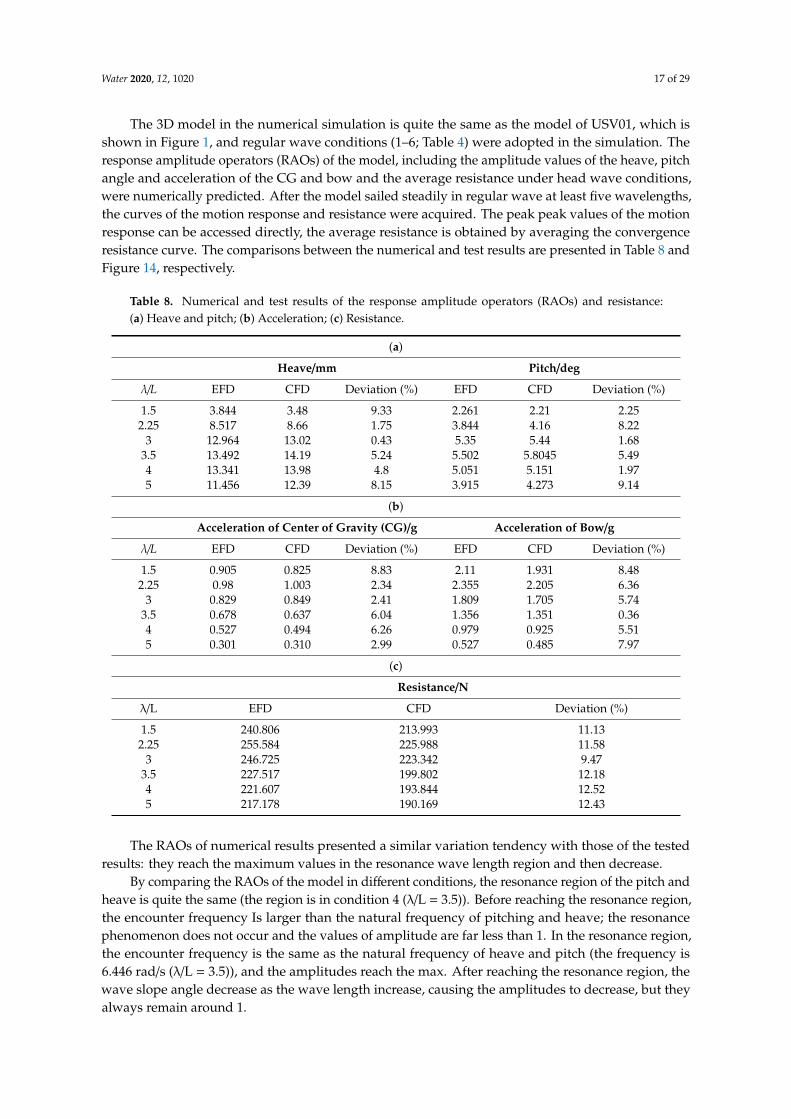
The 3D model in the numerical simulation is quite the same as the model of USV01, which isshown in Figure 1, and regular wave conditions (1–6; Table 4) were adopted in the simulation. Theresponse amplitude operators (RAOs) of the model, including the amplitude values of the heave, pitchangle and acceleration of the CG and bow and the average resistance under head wave conditions,were numerically predicted. After the model sailed steadily in regular wave at least five wavelengths,the curves of the motion response and resistance were acquired. The peak peak values of the motionresponse can be accessed directly, the average resistance is obtained by averaging the convergenceresistance curve. The comparisons between the numerical and test results are presented in Table 8 andFigure 14, respectively.

Table 8. Numerical and test results of the response amplitude operators (RAOs) and resistance:(a) Heave and pitch; (b) Acceleration; (c) Resistance.

(a)

Heave/mm Pitch/deg

λ/L EFD CFD Deviation (%) EFD CFD Deviation (%)

1.5 3.844 3.48 9.33 2.261 2.21 2.252.25 8.517 8.66 1.75 3.844 4.16 8.22

3 12.964 13.02 0.43 5.35 5.44 1.683.5 13.492 14.19 5.24 5.502 5.8045 5.494 13.341 13.98 4.8 5.051 5.151 1.975 11.456 12.39 8.15 3.915 4.273 9.14

(b)

Acceleration of Center of Gravity (CG)/g Acceleration of Bow/g

λ/L EFD CFD Deviation (%) EFD CFD Deviation (%)

1.5 0.905 0.825 8.83 2.11 1.931 8.482.25 0.98 1.003 2.34 2.355 2.205 6.36

3 0.829 0.849 2.41 1.809 1.705 5.743.5 0.678 0.637 6.04 1.356 1.351 0.364 0.527 0.494 6.26 0.979 0.925 5.515 0.301 0.310 2.99 0.527 0.485 7.97

(c)

Resistance/N

λ/L EFD CFD Deviation (%)

1.5 240.806 213.993 11.132.25 255.584 225.988 11.58

3 246.725 223.342 9.473.5 227.517 199.802 12.184 221.607 193.844 12.525 217.178 190.169 12.43

The RAOs of numerical results presented a similar variation tendency with those of the testedresults: they reach the maximum values in the resonance wave length region and then decrease.

By comparing the RAOs of the model in different conditions, the resonance region of the pitch andheave is quite the same (the region is in condition 4 (λ/L = 3.5)). Before reaching the resonance region,the encounter frequency Is larger than the natural frequency of pitching and heave; the resonancephenomenon does not occur and the values of amplitude are far less than 1. In the resonance region,the encounter frequency is the same as the natural frequency of heave and pitch (the frequency is6.446 rad/s (λ/L = 3.5)), and the amplitudes reach the max. After reaching the resonance region, thewave slope angle decrease as the wave length increase, causing the amplitudes to decrease, but theyalways remain around 1.


(a) (b)

(c) (d)

(e)

Figure 14. Comparison of the numerical and tested results: (a) Amplitudes of the heave; (b)

Amplitudes of the pitch; (c) Amplitudes of the acceleration of the CG; (d) Amplitudes of the

acceleration of the bow; (e) Average values of the resistance.

The RAOs of numerical results presented a similar variation tendency with those of the tested

results: they reach the maximum values in the resonance wave length region and then decrease.

By comparing the RAOs of the model in different conditions, the resonance region of the pitch

and heave is quite the same (the region is in condition 4 (λ/L = 3.5)). Before reaching the resonance

Figure 14. Comparison of the numerical and tested results: (a) Amplitudes of the heave; (b) Amplitudesof the pitch; (c) Amplitudes of the acceleration of the CG; (d) Amplitudes of the acceleration of the bow;(e) Average values of the resistance.

The resonance region of the acceleration of the CG and bow is different (the region is in condition2 (λ/L = 2.25)). Under the short wave length conditions (λ/L ≤ 2.25), the vertical motion of the modelis more intense due to the larger wave slope angle and wave disturbances, when the λ/L reaches 3.5,

Water 2020, 12, 1020 19 of 29

the pitch motion become more intense due to the resonance phenomenon. This indicates that theresonance region of the acceleration shifts to the shorter wave length direction compared with thatof heave and pitch, the natural frequency of the vertical motion of the vessel is larger than that ofpitch and heave, and the natural frequency of vertical motion is 9.261 rad/s (λ/L = 2.25). Under anycondition, the amplitudes of the acceleration of the bow are significantly greater than that of CG. Thisindicates that the bow will slap on the free surface during navigation, and the excessive value of bowacceleration may threaten navigation safety.

The deviation of the numerical method is mainly due to the deformation of the grid and thecomplex flow fields around the model. The relative deviations of the numerical methods are greatlyaffected by the wave conditions. Before reaching the resonance region, the deviation between thecalculated and test values is small. However, when the waves reach the resonance region, theamplitudes of the heave and pitch increased gradually, the motion of the model in the waves becomemore intense, and the deviation become larger.

The maximum deviations of the calculated heave, pitch, and acceleration of the CG and bow are9.33%, 9.14%, 8.83%, and 8.48%, respectively. The average deviations are 4.95%, 4.79%, 4.81%, and5.73%, respectively. All the deviations of the RAOs are less than 10%. The deviations of the numericalresults of the RAOs all become larger in their resonance regions. In the short wave length condition(λ/L = 1.5 and 2.25), the short encountering period increases the frequency of the vertical motion, andthe amplitudes of the acceleration increase sharply. This makes the nonlinear characteristics of thevertical motion increase sharply, and the deviation between the numerical and test results becomelarger in these conditions. As for the pitch and heave, the variation in the deviations is similar to thatof the acceleration, but the wave length of their resonance region is larger.

In terms of average resistance, the values of average resistance are similar in any condition, thedeviation between the numerical and test values is similar in different conditions, and the numericalresults of the average resistance of the vessel in regular wave are all lower than those of the test results.The maximum value is 12.54%, the average value is 11.55%. Meanwhile, compared with the RAOs,the deviation of the resistance is greater. In wave conditions, the proportion of hull wave-makingresistance in the total resistance is large as the flow field around the hull becomes more complicated bythe wave disturbance. The grids around the hull cannot accurately track the free surface, the complexflow field around the hull brings deviation to the numerical prediction of wave-making resistance, thismakes the numerical result of the resistance mean a certain deviation compared with the experimentalvalue, but the variation tendency are similar.

Summing up the above, the numerical method accurately predicted the variation trends of themodel’s motion response in regular wave. Compared with the corresponding test results, the relativedeviations of the numerical results of the RAOs are less than 10%. This shows that the numericalmethod has a high accuracy in predicting the motion response of the model in regular wave. However,increasing nonlinear characteristics of the motion will make deviation of the numerical results becomelarger. Meanwhile, the complex flow field around the hull made it difficult to predict the wave-makingresistance accurately and the deviation of the numerical results of the resistance are larger than that ofthe RAOs.

5. Numerical Simulation of Planing Craft in Regular Wave with Large Wave Height

Based on the numerical method which was been validated in Section 4, the low steaming of smallplaning craft under regular wave with large wave height is numerical analyzed.

The USV01 is designed for high-speed offshore navigation, its seakeeping is not enough to ensuresafe navigation under regular wave with large wave height. The subsequent numerical simulation inlarge wave height conditions are not suitable to take USV01 as the simulation object.

A new small planing craft with better seakeeping is selected as the object of numerical simulation.The vessel’s length is 6 m, displacement is 1.8t, the deadrise angle at the stern is 24 deg, and the model

Water 2020, 12, 1020 20 of 29

scale is set at 1:3. The vessel has a larger deadrise angle and more drafts, in pitching and heave motioncaused by wave disturbance, the hull can provide more damping.

To compare and validate the seakeeping performance of the new planing craft, the model ofUSV01 was scaled down to the same size and displacement as the new planing craft. Under the samewave conditions, the sailing of the two vessels under large wave height is predicted and compared.

The scaled model of USV01 is selected as prototype. The new vessel improved in seakeepingcompared with the prototype, the new vessel is named as improved vessel.

The hull and specific parameters of the improved vessel are presented in Figure 15 andTable 9, respectively.

Water 2020, 12, x 20 of 30

5. Numerical Simulation of Planing Craft in Regular Wave with large Wave Height

Based on the numerical method which was been validated in section 4, the low steaming of small

planing craft under regular wave with large wave height is numerical analyzed.

The USV01 is designed for high‐speed offshore navigation, its seakeeping is not enough to

ensure safe navigation under regular wave with large wave height. The subsequent numerical

simulation in large wave height conditions are not suitable to take USV01 as the simulation object.

A new small planing craft with better seakeeping is selected as the object of numerical

simulation. The vessel’s length is 6 m, displacement is 1.8t, the deadrise angle at the stern is 24 deg,

and the model scale is set at 1:3. The vessel has a larger deadrise angle and more drafts, in pitching

and heave motion caused by wave disturbance, the hull can provide more damping.

To compare and validate the seakeeping performance of the new planing craft, the model of

USV01 was scaled down to the same size and displacement as the new planing craft. Under the same

wave conditions, the sailing of the two vessels under large wave height is predicted and compared.

The scaled model of USV01 is selected as prototype. The new vessel improved in seakeeping

compared with the prototype, the new vessel is named as improved vessel.

The hull and specific parameters of the improved vessel are presented in Figure 15 and Table 9,

respectively.

Table 9. Model parameters of the improved vessel.


Model scale k 1:3

Length overall L 2 m

Beam overall B 0.54 m

Mouded depth h 0.256 m

Displacement Δ 66.67 kg

Draft d 0.147 m

Longitudinal position of the center of gravity LCG 0.82 m

Deadrise angle 𝛽 24 deg

Figure 15. Threedimensional (3D) model and line plan of the improved vessel. Figure 15. Threedimensional (3D) model and line plan of the improved vessel.

Table 9. Model parameters of the improved vessel.

Main Feature Symbol Value

Model scale k 1:3Length overall L 2 mBeam overall B 0.54 m


Draft d 0.147 mLongitudinal position of the center of gravity LCG 0.82 m


The model of USV01 is scaled down to the size shown in Table 10, but the shape remains the same.The low steaming of the two vessels in the same conditions is numerically simulated. The regular

wave conditions refer to moderate sea conditions. The wave height of the moderate sea conditionsranges from 1.25 m to 2.5 m. In the numerical simulation, the scale ratio is 1:3, the wave height ofregular wave is set at 0.45 m, and the wave length range from 2 L to 6 L. The parameters of regularwave are shown in Table 11.

Water 2020, 12, 1020 21 of 29

Table 10. Model parameters of the prototype.

Main Feature Symbol Value

Length overall L 2 mBeam overall B 0.67 m


Draft d 0.118 mLongitudinal position of the center of gravity LCG 0.82 m


Table 11. The matrix of regular wave with large wave height.

No U (m/s) Fn H (m) λ/L λ (m) ω (rad/s) H/λ

7 2 0.46 0.45 2 4 7.316 0.11258 2 0.46 0.45 3 6 5.391 0.0759 2 0.46 0.45 4 8 4.390 0.0562510 2 0.46 0.45 5 10 3.749 0.04511 2 0.46 0.45 6 12 3.324 0.0375

6. Results

6.1. The Influence of Wave Length on the Navigation Configuration

To study the seakeeping of the two vessels, the sailing of the prototype and improved vesselin conditions 7 to 11 were simulated, their motion responses were compared. The comparisons arepresented in Table 12 and Figure 16, respectively.

Table 12. RAOs of the prototype and improved vessel: (a) Heave and pitch; (b) Acceleration

(a)

Amplitude of Heave (m) Amplitude of Pitch (deg)

λ/L prototype improved vessel prototype improved vessel2 0.103 0.118 6.825 7.8953 0.213 0.209 8.764 10.6854 0.228 0.209 9.653 9.445 0.233 0.208 8.942 7.8356 0.235 0.207 7.483 6.195

(b)

Amplitude of Acceleration of CG (g) Amplitude of Acceleration of Bow (g)

λ/L prototype improved vessel prototype improved vessel2 0.574 0.651 1.017 1.2783 0.677 0.659 1.411 1.3094 0.531 0.503 0.871 0.7835 0.398 0.367 0.617 0.5496 0.272 0.251 0.451 0.347

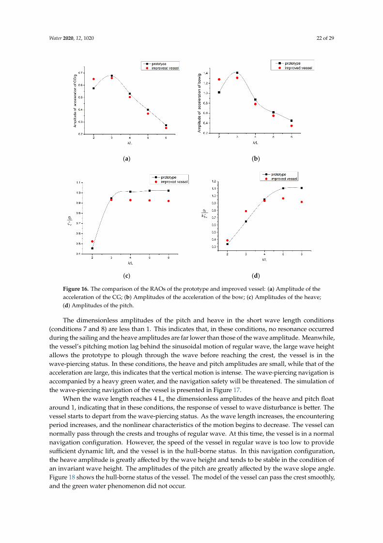
Figure 16 indicates that the motion tendency of the prototype and improved vessel are similar:As the wave length increased, the amplitudes of the pitch and acceleration began to decrease graduallyafter reaching the resonance region, while the amplitudes of heave tend to remain stable.


(a) (b)

(c) (d)

Figure 16. The comparison of the RAOs of the prototype and improved vessel: (a) Amplitude of the

acceleration of the CG; (b) Amplitudes of the acceleration of the bow; (c) Amplitudes of the heave; (d)

Amplitudes of the pitch.

Figure 16 indicates that the motion tendency of the prototype and improved vessel are similar:

As the wave length increased, the amplitudes of the pitch and acceleration began to decrease

gradually after reaching the resonance region, while the amplitudes of heave tend to remain stable.

The dimensionless amplitudes of the pitch and heave in the short wave length conditions

(conditions 7 and 8) are less than 1. This indicates that, in these conditions, no resonance occurred

during the sailing and the heave amplitudes are far lower than those of the wave amplitude.

Meanwhile, the vesselʹs pitching motion lag behind the sinusoidal motion of regular wave, the large wave height allows the prototype to plough through the wave before reaching the crest, the vessel is

in the wave‐piercing status. In these conditions, the heave and pitch amplitudes are small, while that

of the acceleration are large, this indicates that the vertical motion is intense. The wave‐piercing

navigation is accompanied by a heavy green water, and the navigation safety will be threatened. The

simulation of the wave‐piercing navigation of the vessel is presented in Figure 17.

Figure 16. The comparison of the RAOs of the prototype and improved vessel: (a) Amplitude of theacceleration of the CG; (b) Amplitudes of the acceleration of the bow; (c) Amplitudes of the heave;(d) Amplitudes of the pitch.

The dimensionless amplitudes of the pitch and heave in the short wave length conditions(conditions 7 and 8) are less than 1. This indicates that, in these conditions, no resonance occurredduring the sailing and the heave amplitudes are far lower than those of the wave amplitude. Meanwhile,the vessel’s pitching motion lag behind the sinusoidal motion of regular wave, the large wave heightallows the prototype to plough through the wave before reaching the crest, the vessel is in thewave-piercing status. In these conditions, the heave and pitch amplitudes are small, while that of theacceleration are large, this indicates that the vertical motion is intense. The wave-piercing navigation isaccompanied by a heavy green water, and the navigation safety will be threatened. The simulation ofthe wave-piercing navigation of the vessel is presented in Figure 17.

When the wave length reaches 4 L, the dimensionless amplitudes of the heave and pitch floataround 1, indicating that in these conditions, the response of vessel to wave disturbance is better. Thevessel starts to depart from the wave-piercing status. As the wave length increases, the encounteringperiod increases, and the nonlinear characteristics of the motion begins to decrease. The vessel cannormally pass through the crests and troughs of regular wave. At this time, the vessel is in a normalnavigation configuration. However, the speed of the vessel in regular wave is too low to providesufficient dynamic lift, and the vessel is in the hull-borne status. In this navigation configuration,the heave amplitude is greatly affected by the wave height and tends to be stable in the condition ofan invariant wave height. The amplitudes of the pitch are greatly affected by the wave slope angle.Figure 18 shows the hull-borne status of the vessel. The model of the vessel can pass the crest smoothly,and the green water phenomenon did not occur.

Water 2020, 12, 1020 23 of 29

Water 2020, 12, x 23 of 30

(a) (b)

(c).

Figure 17. The simulation of the sailing of the improved vessel in the wave‐piercing status: (a) Free

surface; (b) Gas–liquid phase diagram; (c) Free surface representation of the hull.

When the wave length reaches 4 L, the dimensionless amplitudes of the heave and pitch float

around 1, indicating that in these conditions, the response of vessel to wave disturbance is better. The

vessel starts to depart from the wave‐piercing status. As the wave length increases, the encountering

period increases, and the nonlinear characteristics of the motion begins to decrease. The vessel can

normally pass through the crests and troughs of regular wave. At this time, the vessel is in a normal

navigation configuration. However, the speed of the vessel in regular wave is too low to provide

sufficient dynamic lift, and the vessel is in the hull‐borne status. In this navigation configuration, the

heave amplitude is greatly affected by the wave height and tends to be stable in the condition of an

invariant wave height. The amplitudes of the pitch are greatly affected by the wave slope angle.

Figure 18 shows the hull‐borne status of the vessel. The model of the vessel can pass the crest

smoothly, and the green water phenomenon did not occur.

Figure 17. The simulation of the sailing of the improved vessel in the wave-piercing status: (a) Freesurface; (b) Gas–liquid phase diagram; (c) Free surface representation of the hull.

Water 2020, 12, x 24 of 30

(a) (b)

(c)

Figure 18. The simulation of the sailing of an improved vessel in the hull‐borne status: (a) Free surface; (b) Gas–liquid phase diagram; (c) Free surface representation of the hull.

The dimensions of the improved vessel are the same as those of the prototype, and the motion

trends are consistent in the same condition, both of which have the wave‐piercing status and hull‐

borne status.

In the wave‐piercing status, the RAOs of the improved vessel are slightly larger than those of

the prototype, and while the two vessels are similar in size, the large deadrise angle of the improved

vessel makes its pitching period shorter, allowing the vessel to better respond to wave disturbances.

Due to the large wave height and short encountering period, the improved vessel is also in the wave‐

piercing status, and because of the good response of the improved vessel to the waves, the

phenomenon of green water on deck during navigation will be greatly reduced. Therefore, the

seakeeping of the improved vessel is better than that of the prototype in wave‐piercing status.

When the vessels are in the hull‐borne status, the amplitudes of the heave and pitch become

larger, compared with those in the wave‐piercing status, and the amplitude of the acceleration

decreases sharply. Due to the better seakeeping of the improved vessel, the hull is able to provide

more pitch damping under the regular wave, compared with the prototype. After entering the hull‐

borne status, the RAOs of the improved vessel are all smaller than those of the prototype in the same

wave conditions.

Summing up the above, the improved vessel provides a better seakeeping performance in both

the wave‐piercing and hull‐borne statuses. In the wave‐piercing status, the design of the improved

vessel can effectively reduce the occurrence of wave‐piercing and green water; in the hull‐borne

status, the RAOs of the vessel sailing in regular wave are reduced.

6.2. The Influence of Speed on the Navigation Configuration

To study the influence of speed on the RAOs of improved vessel, the sailing of the improved

vessel at different speeds and with different wave lengths was simulated. Another speed (U = 3 m/s)

is selected. The wave matrix is shown in Table 13.

Figure 18. The simulation of the sailing of an improved vessel in the hull-borne status: (a) Free surface;(b) Gas–liquid phase diagram; (c) Free surface representation of the hull.

The dimensions of the improved vessel are the same as those of the prototype, and the motion trendsare consistent in the same condition, both of which have the wave-piercing status and hull-borne status.

Water 2020, 12, 1020 24 of 29

In the wave-piercing status, the RAOs of the improved vessel are slightly larger than those of theprototype, and while the two vessels are similar in size, the large deadrise angle of the improved vesselmakes its pitching period shorter, allowing the vessel to better respond to wave disturbances. Due tothe large wave height and short encountering period, the improved vessel is also in the wave-piercingstatus, and because of the good response of the improved vessel to the waves, the phenomenon ofgreen water on deck during navigation will be greatly reduced. Therefore, the seakeeping of theimproved vessel is better than that of the prototype in wave-piercing status.

When the vessels are in the hull-borne status, the amplitudes of the heave and pitch become larger,compared with those in the wave-piercing status, and the amplitude of the acceleration decreasessharply. Due to the better seakeeping of the improved vessel, the hull is able to provide more pitchdamping under the regular wave, compared with the prototype. After entering the hull-borne status,the RAOs of the improved vessel are all smaller than those of the prototype in the same wave conditions.

Summing up the above, the improved vessel provides a better seakeeping performance in boththe wave-piercing and hull-borne statuses. In the wave-piercing status, the design of the improvedvessel can effectively reduce the occurrence of wave-piercing and green water; in the hull-borne status,the RAOs of the vessel sailing in regular wave are reduced.

6.2. The Influence of Speed on the Navigation Configuration

To study the influence of speed on the RAOs of improved vessel, the sailing of the improvedvessel at different speeds and with different wave lengths was simulated. Another speed (U = 3 m/s) isselected. The wave matrix is shown in Table 13.

The sailing of the improved vessel in conditions 7–11 and 12–16 were numerically simulated andcompared. The amplitude values of the motion response of model are obtained, and a dimensionlesstreatment is also carried out. A comparison of the RAOs of the vessel at two speeds is presented inTable 14 and Figure 19, respectively.

Table 13. The parameters of regular wave, in which U = 3 m/s.


12 3 0.69 0.45 2 4 8.897 0.112513 3 0.69 0.45 3 6 6.440 0.07514 3 0.69 0.45 4 8 5.177 0.0562515 3 0.69 0.45 5 10 4.392 0.04516 3 0.69 0.45 6 12 3.845 0.0375

Table 14. RAOs of the improved vessel at different speeds and with different wave lengths: (a) Heaveand pitch; (b) Acceleration.

(a)


λ/L Fn = 0.46 Fn = 0.69 Fn = 0.46 Fn = 0.692 0.118 0.097 7.895 6.5973 0.209 0.232 10.685 10.4344 0.209 0.246 9.44 10.2255 0.208 0.244 7.835 8.6736 0.207 0.242 6.195 7.465

(b)


λ/L Fn = 0.46 Fn = 0.69 Fn = 0.46 Fn = 0.692 0.651 0.771 1.278 2.0593 0.659 0.918 1.309 2.7094 0.503 0.752 0.783 1.4035 0.367 0.612 0.549 0.7836 0.251 0.481 0.347 0.574


(a) (b)

(c) (d)

Figure 19. Comparison of the RAOs at two speeds: (a) Amplitudes of the acceleration of the CG; (b)

Amplitudes of the acceleration of the bow; (c) Amplitudes of the heave; (d) Amplitudes of the pitch.

As Figure 19 shows, there are still two kinds of navigation configurations: the wave‐piercing

and hull‐borne statuses. Comparing the RAOs of the improved vessel in the same wave condition at

different speeds, speed has an obvious effect on the RAOs of the vessel. In terms of heave, when λ/L

＞ 3, the vessel is in the hull‐borne status. Increasing the speed makes the hull generate more

dynamic lift, and this greatly increase the heave amplitudes of the vessel. However, when the wave

length decreases, the vessel goes into the wave‐piercing status, and the effect of the speed on the

heave is opposite to that in the hull‐borne status. Meanwhile, the effect of the speed on pitch is

consistent with that of the heave in any condition, but the effect is weaker. In terms of the acceleration,

the acceleration amplitudes of t vessel at 3 m/s (Fn = 0.69) are larger than that of the vessel at 2 m/s

(Fn = 0.46) in any condition, and the speed has a more obvious influence on the acceleration,

compared with the heave and pitch.

For further study, the influence of speed on the RAOs of improved vessel in the wave‐piercing

and hull‐borne statuses have been numerically predicted. The wave conditions where the wave

height is 0.45 m, λ/L = 3 and 6 are selected, λ/L = 3, the improved vessel is in the wave‐piercing status,

and when λ/L = 6, the improved vessel is in the hull‐borne status. The wave matrix is shown in Table

15. The RAOs of the improved vessel are obtained, based on the numerical method, and a comparison

of RAOs at different speeds is presented in Figure 20 and Table 16.

Figure 19. Comparison of the RAOs at two speeds: (a) Amplitudes of the acceleration of the CG;(b) Amplitudes of the acceleration of the bow; (c) Amplitudes of the heave; (d) Amplitudes of the pitch.

As Figure 19 shows, there are still two kinds of navigation configurations: the wave-piercingand hull-borne statuses. Comparing the RAOs of the improved vessel in the same wave condition atdifferent speeds, speed has an obvious effect on the RAOs of the vessel. In terms of heave, when λ/L > 3,the vessel is in the hull-borne status. Increasing the speed makes the hull generate more dynamic lift,and this greatly increase the heave amplitudes of the vessel. However, when the wave length decreases,the vessel goes into the wave-piercing status, and the effect of the speed on the heave is opposite to thatin the hull-borne status. Meanwhile, the effect of the speed on pitch is consistent with that of the heavein any condition, but the effect is weaker. In terms of the acceleration, the acceleration amplitudes of tvessel at 3 m/s (Fn = 0.69) are larger than that of the vessel at 2 m/s (Fn = 0.46) in any condition, and thespeed has a more obvious influence on the acceleration, compared with the heave and pitch.

For further study, the influence of speed on the RAOs of improved vessel in the wave-piercingand hull-borne statuses have been numerically predicted. The wave conditions where the wave heightis 0.45 m, λ/L = 3 and 6 are selected, λ/L = 3, the improved vessel is in the wave-piercing status, andwhen λ/L = 6, the improved vessel is in the hull-borne status. The wave matrix is shown in Table 15.The RAOs of the improved vessel are obtained, based on the numerical method, and a comparison ofRAOs at different speeds is presented in Figure 20 and Table 16.

Water 2020, 12, 1020 26 of 29

Table 15. The regular wave matrix at different speeds.


17 2 0.46 0.45 3 6 5.391 0.07518 3 0.69 0.45 3 6 6.440 0.07519 4 0.92 0.45 3 6 7.489 0.07520 5 1.15 0.45 3 6 8.539 0.07521 6 1.39 0.45 3 6 9.594 0.07522 2 0.46 0.45 6 12 3.324 0.037523 3 0.69 0.45 6 12 3.845 0.037524 4 0.92 0.45 6 12 4.367 0.037525 5 1.15 0.45 6 12 4.888 0.037526 6 1.39 0.45 6 12 5.411 0.0375Water 2020, 12, x 28 of 30

(a) (b)

(c) (d)

Figure 20. Comparison of the RAOs under different navigation configurations: (a) Amplitudes of the

acceleration of the CG; (b) Amplitudes of the acceleration of the bow; (c) Amplitudes of the heave; (d)

Amplitudes of the pitch.

As Figure 20 shows, the effect of increasing the speed is completely opposite to that of changing

the navigation configuration. In the conditions where the wave length is 3 L, U = 2 m/s (Fn = 0.46),

and the vessel is in the wave‐piercing status, the amplitudes of the heave and pitch decrease sharply

as the speed increases. When the wave length reaches 3 L, the period of the encounter decreases with

the increasing of the speed, while the pitch period of the vessel remains unchanged. This means that,

with the increasing of the speed, the gap between the encounter period and the resonance period

increases, and the resonance phenomenon gradually becomes weaker, the amplitudes begin to

decrease, the nonlinear characteristics of pitch increase, and the wave‐piercing phenomenon of the

vessel becomes more obvious, leading to more green water.

In the hull‐borne status (λ/L = 6), the amplitudes of the heave and pitch both increase with the

increasing of the speed. Compared with the wave‐piercing status, amplitudes of the vessel in the

hull‐borne status are much higher than those in the wave‐piercing status. With the increasing of the

speed, the lift force received by the craft gradually increases, making the RAOs of the vessel in regular

wave increase obviously.

In terms of the acceleration, the influence of the speed in different navigation configurations is

quite the same, while in the wave‐piercing status, the influence of the speed on the acceleration is

more obvious. The amplitudes of the acceleration of the vessel increase with the increasing of the

speed in any condition, and the increase will become sharp at a high speed. The amplitudes of the

acceleration of the vessel in the wave‐piercing status (λ/L = 3) are always larger than that in the hull‐

borne status (λ/L = 6). This shows that in the wave‐piercing status, the pitching motion is more

intense, and the nonlinear characteristics of the motion increase. The influence of the speed on the

Figure 20. Comparison of the RAOs under different navigation configurations: (a) Amplitudes of theacceleration of the CG; (b) Amplitudes of the acceleration of the bow; (c) Amplitudes of the heave;(d) Amplitudes of the pitch.

Water 2020, 12, 1020 27 of 29

Table 16. The RAOs of the improved vessel at different speeds: (a) Heave and pitch; (b) Acceleration.

(a)


Fn λ/L = 3 λ/L = 6 λ/L = 3 λ/L = 60.46 0.209 0.207 10.685 6.1590.69 0.232 0.242 10.434 7.4650.92 0.196 0.255 8.745 7.6511.15 0.171 0.2704 6.951 8.4081.39 0.142 0.3035 6.115 9.483

(b)


Fn λ/L = 3 λ/L = 6 λ/L = 3 λ/L = 60.46 0.659 0.251 1.309 0.3470.69 0.918 0.481 2.709 0.5740.92 1.583 0.557 4.022 0.7661.15 2.193 0.712 4.788 1.2761.39 2.436 1.038 4.871 2.381

As Figure 20 shows, the effect of increasing the speed is completely opposite to that of changingthe navigation configuration. In the conditions where the wave length is 3 L, U = 2 m/s (Fn = 0.46), andthe vessel is in the wave-piercing status, the amplitudes of the heave and pitch decrease sharply as thespeed increases. When the wave length reaches 3 L, the period of the encounter decreases with theincreasing of the speed, while the pitch period of the vessel remains unchanged. This means that, withthe increasing of the speed, the gap between the encounter period and the resonance period increases,and the resonance phenomenon gradually becomes weaker, the amplitudes begin to decrease, thenonlinear characteristics of pitch increase, and the wave-piercing phenomenon of the vessel becomesmore obvious, leading to more green water.

In the hull-borne status (λ/L = 6), the amplitudes of the heave and pitch both increase with theincreasing of the speed. Compared with the wave-piercing status, amplitudes of the vessel in thehull-borne status are much higher than those in the wave-piercing status. With the increasing of thespeed, the lift force received by the craft gradually increases, making the RAOs of the vessel in regularwave increase obviously.

In terms of the acceleration, the influence of the speed in different navigation configurations isquite the same, while in the wave-piercing status, the influence of the speed on the acceleration is moreobvious. The amplitudes of the acceleration of the vessel increase with the increasing of the speed inany condition, and the increase will become sharp at a high speed. The amplitudes of the accelerationof the vessel in the wave-piercing status (λ/L = 3) are always larger than that in the hull-borne status(λ/L = 6). This shows that in the wave-piercing status, the pitching motion is more intense, and thenonlinear characteristics of the motion increase. The influence of the speed on the acceleration of CGand bow is consistent. However, the amplitude of the acceleration of the bow increases quite sharplyas the speed continues to increase, indicating that the nonlinear characteristics of the motion of thebow at a high speed increase sharply, which will greatly endanger the navigation safety.

Summing up the above, increasing the speed will increase the nonlinear characteristics of themotion in any condition: in the wave-piercing status, the occurrence of wave-piercing and green waterwill become more serious, in the hull-borne status, the RAOs will increase sharply. This indicates thatreducing the speed is the most effective means to ensure navigation safety under regular wave withlarge wave height.

Water 2020, 12, 1020 28 of 29

7. Conclusions

This paper presents a seakeeping analysis of planing craft, based on numerical and experimentalmethods. In order to validate numerical method, the sailing of USV01 was numerically simulated,based on the RANS solver and overset method. The numerical results of the RAOs were comparedwith the corresponding test results, and the overall uncertainty was within 10%. The deviation of thenumerical method became slightly larger in the resonance region, especially for the acceleration. Theseresults indicate that the numerical method has a high accuracy in simulating the seakeeping test ofplaning craft. Additionally, the numerical prediction of wave-making resistance has a slightly largerdeviation due to complex flow field around the hull.

For further study on the seakeeping performance of vessels in regular wave with large waveheight, a new small size planing craft with better seakeeping performance is selected for numericalsimulation, and the vessel is named as improved vessel, the model of USV01 shrunk to the same size asimproved vessel and named as prototype. The low steaming of the prototype and improved vessel inthe same conditions were numerically simulated and compared. Under the influence of the large waveheight and different wave lengths, there are two navigation configurations in the sailing of the vessels:The wave-piercing and hull-borne status. In the wave-piercing status, the vessel’s pitching motion lagsbehind the sinusoidal motion of regular wave, and there is no resonance phenomenon. The pitch andheave amplitudes are small, and the vessel traverses the waves, accompanied by severely green water.In the hull-borne status, the amplitudes of the pitch and heave are affected by the wave conditions.Compared with the prototype, the improved vessel shows a better seakeeping performance in bothnavigation configurations: in the wave-piercing status, the phenomenon of green water will be greatlyreduced with the improved vessel, and in the hull-borne status, the RAOs of the improved vessel arelower than those of the prototype in the same wave conditions. For further study, the influence of thespeed on the RAOs of the improved vessel in different navigation configurations will be analyzed. Theincreasing of the speed increases the nonlinear characteristics of the vessel’s motion in regular waveand in both the wave-piercing and hull-borne statuses. However, in different navigation configurations,the effect of the speed on the RAOs will be different, and reducing speed is the most effective means toensure the navigation safety of planing craft under regular wave with large wave height.

Author Contributions: Conceptualization, X.B., J.Z. and Y.S.; Formal analysis, J.Z. and Y.S.; Methodology, X.B.;Project administration, J.Z.; Software, X.B.; Validation, X.B.; Writing—original draft, X.B.; Writing—review &editing, J.Z. and Y.S. All authors have read and agreed to the published version of the manuscript.

Funding: This research was financially funded by the National Natural Science Foundation of China (Grant No.51409054), the Foundation Research Funds for the Central Universities (Grant No. HEUCF180101).

Acknowledgments: The author would like to express his gratitude to the reviewers for their suggestions andobservations that helped in improving the present work.

Conflicts of Interest: The authors declare no conflicts of interest.

References

1. Faltinsen, O.M. Hydrodynamics of High-Speed Marine Vehicles; National Defense Industry Press: Beijing,China, 2007.

2. Dong, W.-C.; Guo, R.-X. State of the art of prediction on resistance of planing crafts. Ship Mech. 2000, 4, 68–81.3. Diez, M.; Serani, A.; Campana, E.F. CFD-based stochastic optimization of a destroyer hull form for realistic

ocean operations. In Proceedings of the 14th International Conference on Fast Sea Transportation, Nantes,France, 27–29 September 2017; pp. 1–9.

4. Campana, E.F.; Diez, M.; Liuzzi, G.; Lucidi, S.; Pellegrini, R.; Piccialli, V.; Rinaldi, F.; Serani, A. A multi-objectiveDIRECT algorithm for ship hull optimization. Comput. Optim. Appl. 2019, 71, 53–72. [CrossRef]

5. AZCUETA, R. Computational of Turbulent Free Surface Flows Around Ships and Floating Bodies; TechnicalUniversity Hamburg-Harburg: Hamburg, Germany, 2001.

6. Caponnetto, M. Practical CFD simulations for planing hulls. In Proceedings of the Second International EuroConference on High Performance Marine Vehicles, Hamburg, Germany, 2–5 May 2001; pp. 128–138.

http://dx.doi.org/10.1007/s10589-017-9955-0

Water 2020, 12, 1020 29 of 29

7. Weymouth, G.D.; Wilson, R.V.; Stern, F. RANS computational fluid dynamics predictions of pitch and heaveship motions in head seas. J. Ship Res. 2005, 49, 80–97.

8. Sun, H.; Ma, W.; Zhu, J. Research on grid factor in numerical calculation of planing craft resistance. ShipBuild. China 2015, 56, 170–178.

9. Su, Y.-m.; Zhao, J.-x.; Chen, Q.-t.; Zhu, W.; Jin, X. Numerical simulation of the planing vessel in regularwaves. Ship Mech. 2013, 17, 583–590.

10. De Marco, A.; Mancini, S.; Miranda, S.; Scognamiglio, R.; Vitiello, L. Experimental and numericalhydrodynamic analysis of a stepped planing hull. Appl. Ocean Res. 2017, 64, 135–154. [CrossRef]

11. Dashtimanesh, A.; Tavakoli, S.; Sahoo, P. A simplified method to calculate trim and resistance of a two-steppedplaning hull. Ships Offshore Struct. 2017, 12 (Suppl. 1), S317–S329. [CrossRef]

12. Ikeda, Y.; Katayama, T. Porpoising oscillations of very-high-speed marine craft. Phil. Trans. R. Soc. Lond. A2000, 358, 1905–1915. [CrossRef]

13. AZCUETA, R. Steady and unsteady ranse simulations for planing crafts. In Proceedings of the 7thInternational Conference on Fast Sea Transportation, Ischia, Italy, 7–10 October 2003; pp. 41–48.

14. Begovic, E.; Bertorello, C.; Pennino, S. Experimental seakeeping assessment of a warped planing hull modelseries. Ocean Eng. 2014, 83, 1–15. [CrossRef]

15. Begovic, E.; Bertorello, C.; Pennino, S.; Piscopo, V.; Scamardella, A. Statistical analysis of planing hull motionsand accelerations in irregular head sea. Ocean Eng. 2016, 112, 253–264. [CrossRef]

16. Jiang, Y.; Sun, H.; Zou, J.; Hu, A.; Yang, J. Experimental and numerical investigations on hydrodynamic andaerodynamic characteristics of the tunnel of planing trimaran. Appl. Ocean Res. 2017, 63, 1–10. [CrossRef]

17. Jiang, Y.; Sun, H.; Zou, J.; Hu, A.; Yang, J. Analysis of tunnel hydrodynamic characteristics for planingtrimaran by model tests and numerical simulations. Ocean Eng. 2016, 113, 101–110. [CrossRef]

18. Bi, X.; Shen, H.; Zhou, J.; Su, Y. Numerical analysis of the influence of fixed hydrofoil installation position onseakeeping of the planing craft. Appl. Ocean Res. 2019, 90, 101863. [CrossRef]

19. Menter, F.R. Improved Two-Equation Turbulence Models for Aerodynamic Flows; NASA Technical Memorandum:California, CA, USA, 1992.

20. Wang, F. Computational Fluid Dynamics Analysis-Theory and Application of CFD Software; Tsinghua UniversityPress: Beijing, China, 2005.

21. Scardovelli, R.; Zaleski, S. Direct numerical simulation of free-surface and interfacial flow. Annu. Rev. FluidMech. 1999, 31, 567–603. [CrossRef]

22. Hirt, C.W.; Nichols, B.D. Volume of Fluid (VOF) method for the dynamics of free boundary. J. Comput. Phys.1981, 39, 201–225. [CrossRef]

23. Bertorello, C.; Begovic, E.; Mancini, S. Hydrodynamic performances of small sizes swath craft. Brodogr.Shipbuild. 2015, 66, 1–22.

© 2020 by the authors. Licensee MDPI, Basel, Switzerland. This article is an open accessarticle distributed under the terms and conditions of the Creative Commons Attribution(CC BY) license (http://creativecommons.org/licenses/by/4.0/).

http://dx.doi.org/10.1016/j.apor.2017.02.004

http://dx.doi.org/10.1080/17445302.2016.1262809

http://dx.doi.org/10.1098/rsta.2000.0620

http://dx.doi.org/10.1016/j.oceaneng.2014.03.012


http://dx.doi.org/10.1016/j.apor.2016.12.009


http://dx.doi.org/10.1016/j.apor.2019.101863

http://dx.doi.org/10.1146/annurev.fluid.31.1.567

http://dx.doi.org/10.1016/0021-9991(81)90145-5

http://creativecommons.org/

http://creativecommons.org/licenses/by/4.0/.

Xiaosheng Bi, Jiayuan Zhuang * and Yumin Su

Documents

Transcript of Xiaosheng Bi, Jiayuan Zhuang * and Yumin Su