XGBOOSTAS A TIME-SERIES FORECASTING TOOL
20
XGBOOST AS A TIME-SERIES FORECASTING TOOL Filip Wójcik Objectivity Digital Transformation Specialists PhD Student on a Wroclaw University of Economics [email protected]
Transcript of XGBOOSTAS A TIME-SERIES FORECASTING TOOL

XGBOOST AS A TIME-SERIES
FORECASTING TOOL
Filip Wójcik
Objectivity Digital Transformation Specialists
PhD Student on a Wroclaw University of Economics

What is XGboost01
Rossmann – legendary competition
02
Forecasting – training challenges03
Data preparation04
Training method05
Comparison to other models06
Results analysis07
Other data sources08
Summary09
Agenda

What is XGBoost
• Primarily intended for
classification and regression
• Optimizes many different
scoring and error functions
• Supports target functions:
➢ Softmax
➢ Logit
➢ Linear
➢ Poisson
➢ Gamma
Classification & regression algorithm
• Base estimators are decision
trees
• Composite algorithm – an
ensemble
• Booting type algorithm –
increasing weight of harder
examples
• Each tree improves previous
one
Based on trees
• Trees are dependent on each
other
• Parallelization occurs at the
level of a single tree – for
building successive nodes
• XGBoost uses compressed
data format to save memory
Good parallelization

What is XGBoost
Source: http://xgboost.readthedocs.io/en/latest/model.html#tree-ensemble
𝑙 𝑥1, 𝑥2 − cost function
𝑓𝑖 𝑥 − i − th tree builing function
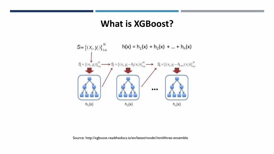
What is XGBoost?
Source: http://xgboost.readthedocs.io/en/latest/model.html#tree-ensemble

Rossmann – legendary competition
• Kaggle.com contest started in 2016r – the goal was to forecast turnover based on
historical values and data from macrosurroundings of stores
• 3303 teams took part
• A significant majority of kernels implemented the Xgboost algorithm
• Evaluation Metric – RMSPE Root mean squared percentage error
RMSPE =1
𝑛
𝑖=1
𝑛𝑦𝑖 − ෝ𝑦𝑖𝑦𝑖
2
• Best score – approx. 10% error
• Typical problem of forecasting – not classification or regression

Forecasting – training challenges
• Two types of variables
➢ Static – describing each store characteristics
➢ Time series– turnover and customer count
• Challenge in training time series forecasting model
➢ Standard cross-validation does not work
➢ Random selection ruins chronology and order
➢ OOB error is not the best estimator anymore
• Huge prediction variance between subsequent runs
• Maintaining order and chronology is crucial to teach the model
➢ Seasonal trends
➢ Autocorrelation
≠

Data preparation
Numerical time indicators
• Number representing Day-Of-week
• Month Number
• Quarter number
Day: 19, month: 3, year: 2015, Q: 1 𝝁𝒒𝟐 = 𝟑𝟖𝟑𝟓, 𝝈𝒒𝟐 = 𝟏𝟖𝟎𝟓Seasonal indices
• Seasonal means and standard
deviations
• Calculated per day-of-
week/week/month/quarter
Additional seasonal indices:
• Moving averages
• Different orders – last day/5-days/2
weeks/etc.

Data preparation
Shop DateDay of
weekMonth Quarter Shop type Promo Assortment Sales 𝜇𝑠𝑎𝑙𝑒𝑠
𝑑𝑎𝑦 𝑜𝑓 𝑤𝑒𝑒𝑘 𝜇𝑠𝑎𝑙𝑒𝑠𝑚𝑜𝑛𝑡ℎ 𝜇𝑠𝑎𝑙𝑒𝑠
𝑞𝑢𝑎𝑟𝑡𝑒𝑟
1 10-01-2016 7 1 1 A True B 1536 954 1100 950
2 15-10-2016 6 10 4 C False A 764 1005 1256 1954
Time - indicators Static variables Seasonal indicesy
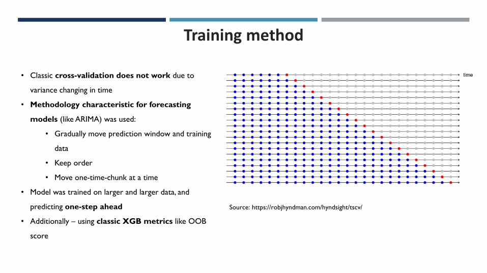
Training method
• Classic cross-validation does not work due to
variance changing in time
• Methodology characteristic for forecasting
models (like ARIMA) was used:
• Gradually move prediction window and training
data
• Keep order
• Move one-time-chunk at a time
• Model was trained on larger and larger data, and
predicting one-step ahead
• Additionally – using classic XGB metrics like OOB
score
Source: https://robjhyndman.com/hyndsight/tscv/

The goal of study and assumptions
Comparison to other models
Comparative study of different forecasting methods using exogenous
(static) variables
Research question
• Systemathic comparison of forecasts
• Is there a statistically SIGNIFICANT difference?
Statistical comparison of prediction quality
• In case of „classic” models – parameters interpretaion
• In case of XGBoost – feature importance calculation
Coefficient importance check
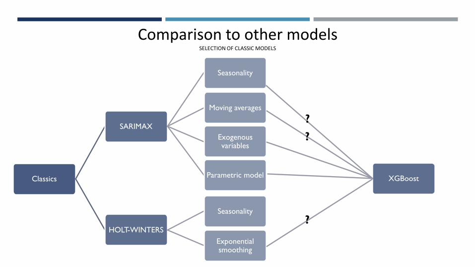
Comparison to other modelsSELECTION OF CLASSIC MODELS
Classics
SARIMAX
Seasonality
Moving averages
Exogenous variables
Parametric model
HOLT-WINTERS
Seasonality
Exponential smoothing
XGBoost
?
?
?

Comparison to other modelsTRAINING METHODS
One model per store
For each store – separate
model was trained
Automatic params tuning
Params for each model were selected
automatically using optimization techniques
(AIC, BIC, RMSPE). Random sample was
manually cross-checked
Missing values interpolation
In case of missing values – polynomial interpolation
was used
One model for full dataset
Experimental study indicated that seasonal indices +
exogenous variables are enough for model to generalize. One
model for full dataset is enough
Regression trees
Base estimators were regression trees and RMSPE – error
function
Time-series validation
One-step Ahead validation technique was used, enriched
with 1000 last observations from ordered dataset
CLASSIC MODELS XGBOOST

Results analysisMetric(median)
SARIMAX Holt-Winters XGBoost
Theil’s
coefficient0.061 0.059 0.1364
𝑅2 0.838 0.54 0.92
RMSPE
(valid.)0.17 0.18 0.13
RMSPE
(leaderboard)0.16 0.367 0.121
ModelsRMSPE
diff
Confidence
from
Confidence
toP-val
XGBoost -
SARIMAX-0.126 -0.141 -0.111 << 0.01
XGBoost - Holt-
Winters-0.218 -0.235 -0.200 << 0.01

Results analysis
0,00% 5,00% 10,00% 15,00% 20,00% 25,00% 30,00% 35,00%
CompetitionDistance
Promo
Store
meanSalesDow
CompetitionOpenSinceMonth
CompetitionOpenSinceYear
day
meanSalesMonth
Promo2SinceYear
Promo2SinceWeek
DayOfWeek
meanCustDow
month
StoreType
meanCustMonth
Promo2
Assortment
PromoInterval
year
meanSalesQ
meanCustQ
SchoolHoliday
quarter
Feature importance
Gain Cover Frequency
Results analysis
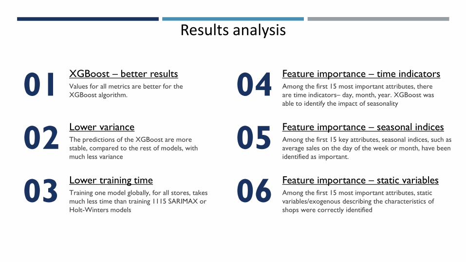
01XGBoost – better resultsValues for all metrics are better for the
XGBoost algorithm. 04Feature importance – time indicatorsAmong the first 15 most important attributes, there
are time indicators– day, month, year. XGBoost was
able to identify the impact of seasonality
02Lower varianceThe predictions of the XGBoost are more
stable, compared to the rest of models, with
much less variance
05Feature importance – seasonal indicesAmong the first 15 key attributes, seasonal indices, such as
average sales on the day of the week or month, have been
identified as important.
03Lower training timeTraining one model globally, for all stores, takes
much less time than training 1115 SARIMAX or
Holt-Winters models
06Feature importance – static variablesAmong the first 15 most important attributes, static
variables/exogenous describing the characteristics of
shops were correctly identified
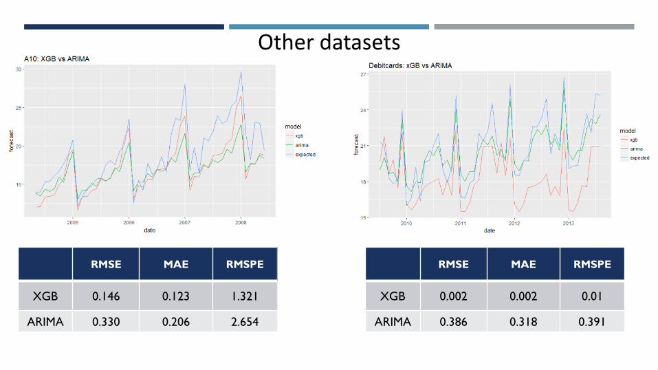
Other datasets
RMSE MAE RMSPE
XGB 0.146 0.123 1.321
ARIMA 0.330 0.206 2.654
RMSE MAE RMSPE
XGB 0.002 0.002 0.01
ARIMA 0.386 0.318 0.391

SummaryThe initial results of the study seem to indicate that XGBoost is well
suited as a tool for forecasting, both in typical time series and in mixed-
character data.
On all data sets tested, XGBoost predictions have low variance and
are stable.
Low variance
The Model is able to recognize trends and seasonal fluctuations, and
the significance of these attributes is confirmed by manual analysis.
Trend and seasonality identification
The Model can simultaneously handle variables of the nature of time
indexes and static exogenous variables
Exogenous variables handling

Papers
Chen, T. & Guestrin, C. (2016) „XGBoost: A scalable tree boosting system”, in Proceedings of the 22nd ACM
SIGKDD International Conference on Knowledge Discovery and Data Mining - KDD ’16. New York, USA:
ACM Press, p. 785–794
Ghosh, R. & Purkayastha, P. (2017) „Forecasting profitability in equity trades using random forest,
support vector machine and xgboost”, in 10th International Conference on Recent Trades in Engineering
Science and Management, p. 473–486.
Gumus, M. & Kiran, M. S. (2017) „Crude oil price forecasting using XGBoost”, in 2017 International
Conference on Computer Science and Engineering (UBMK). IEEE, p. 1100–1103.
Gurnani, M. et al. (2017) „Forecasting of sales by using fusion of machine learning techniques”, in 2017
International Conference on Data Management, Analytics and Innovation (ICDMAI). IEEE, p. 93–101

THANK YOU FOR ATTENTION