CLEARLY BETTER.

XCOR – TODAY’S APPROACH TO DETECTING COMMON PATH DISTORTION

185 AINSLEY DRIVE

SYRACUSE, NY 13210

800.448.1655 / WWW.ARCOMDIGITAL.COM

AD

VA

NC

ED

TE

CH

NO

LO

GY

CLEARLY BETTER. 2

AD

VA

NC

ED

TE

CH

NO

LO

GY

Cable networks are trending further and further towards all-or

majority-digital content. This trend has changed the way CPD

appears to the technician. The days of troubleshooting high

level CPD with a spectrum analyzer by looking for recurring

6 or 8MHz peaks are gone – CPD in today’s network manifests

simply as an elevated return path noise floor, making it

impossible to differentiate CPD from noise and ingress. For

field technicians, the only possible way to troubleshoot CPD

has been to pull pads and disrupt the network in an attempt

to track direction– not a sustainable practice in today’s

competitive market. Arcom Digital’s Xcor technology has

solved this issue by changing the way cable operators

can monitor and troubleshoot Common Path Distortion

(CPD) in the HFC network. Xcor is the ONLY technology

that can accurately identify and track down CPD and

other nonlinear distortion. It is available as part of an

integrated and unique return path monitoring system

called Hunter, or in standalone field test equipment in

the Quiver series of meters. Operationally, Xcor has

paid dividends because of its ability to quickly find the

cause of network impairments. For some operators,

Hunter has re-shaped the entire plant maintenance

methodology, allowing a major shift from Reactive

maintenance to Predictive maintenance. It saves time

and effort, provides clear visibility to impairments

that were previously difficult or impossible to

identify, and results in a better performing, more

reliable plant.

A NEED FOR CHANGE

CLEARLY BETTER. 3

CPD can be quite disruptive for cable operators, and it has been found

that the root causes of CPD sources are frequently the same root

causes of noise and ingress issues. Issues that have been discovered

with Hunter include nodes with missing seizure screws, amplifiers

with loose hardline connectors, waterlogged amplifiers and nodes,

faulty or overloaded amps, faulty terminators, internally rusted taps,

corroded F-connectors, etc., etc. Thousands of devices have been

found – all of which needed to be replaced, and all of which were

causing or would have caused network problems.

Every CPD source is inherently a source of nonlinear distortion. We

use this characteristic to our advantage. Our radar technology deter-

mines exactly where in the system the distortion is coming from.

The radar portion of the system provides the time distance to the

problem. The technician is able to quickly, efficiently, and logically

go to the offending device and fix the problem. The days of spending

weeks locating intermittent problems are gone.

For a radar system to operate within an HFC system three core

elements are required: a transmission of a probing signal in which

energy is propagated towards a target, an echo signal that will travel

back through the network to a receiver, and a relationship between

the probing and echo signal for ranging and detection processing.

THE TECHNOLOGY

CLEARLY BETTER. 4

Xcor utilizes the existing forward QAM channels as the radar probing

signal. As the channels propagate through the network and as they

come across source locations of CPD, intermodulation products are

generated. For any two QAM channels, a second order intermodulation

product will be generated at the difference between the two signals

whenever they travel through a source of CPD. These intermodulation

products that travel through the return network back to the radar

receiver are the echo signals used by the system – they are the second

of the three required elements mentioned above.

Figure 1 is a representation of the second order intermodulation

products created from the digital QAM channels propagating a CPD

source (a nonlinear junction or corrosion cell).

FORWARD PATH SPECTRUM

RETURN PATH SPECTRUM

DIGITAL QAM CHANNELSANALOG CHANNELS

Frequency (MHz)

Frequency (MHz)

48

5 6 12 18 24 30 36 42

550 860

Intermodulation productsfrom digital channels

Detects CPD echo signalsthroughout full spectrum

Return pathspectrum roll-o�

FIG

UR

E 1

CLEARLY BETTER. 5

The last remaining required element is a relationship between the

probing signal and the echo signal. Xcor creates this relationship

through a technique that Arcom Digital has called a CPD Simulator.

All the forward signals in the network are fed to the CPD Simulator.

A snapshot is then taken of the spectrum at a specific moment in

time. The CPD Simulator then calculates what the instantaneous

intermodulation products would look like given the input spectrum.

This calculated signal can be thought of as the T=0 echo. If CPD

occurred at the headend or field connection point, these are the

intermodulation products that would be generated. This process

establishes a relationship between the probing signal and the echo,

which satisfies the third and last required element of the radar system.

All that remains is the signal processing for detection and ranging.

As was mentioned, if there is a CPD source at the headend, it will

match the T=0 echo exactly. Furthermore, CPD occurring in the HFC

network generated from the same signal as used in the CPD Simulator

snapshot will appear identical to the T=0 echo, except that it will be

shifted in time. The remaining task is the process that finds what

this time shift is. The echo is compared with the signal from the CPD

Simulator in order to determine this time delay in which the two

signals are identical – which represents the time distance to the source.

A rough block diagram of the entire Xcor radar system is shown in

Figure 2, and is essentially the same for either the headend or the field

meter implementation.

The Forward signals are input into the Xcor radar through a directional

coupler, or by a network connection when using the Quiver field

meter. These signals then go through a CPD Simulator process in

which intermodulation products are created from filtered forward QAM

channels.The digitized output of the CPD Simulator appears as noise

– however it is not noise because it was generated in a certain fashion

and is not random.

On the right side of the

diagram, the return inputs

from the Hunter switches (or

just a return path test point

connection in the case of the

Quiver) are fed into the Xcor

radar. The digitized output of

these return signals is real noise

from the system – although it

has some special characteristics.

Hidden within this noise is a

particular noise-like pattern,

which is identical to that from

the CPD Simulator but shifted in

time by some unknown amount.

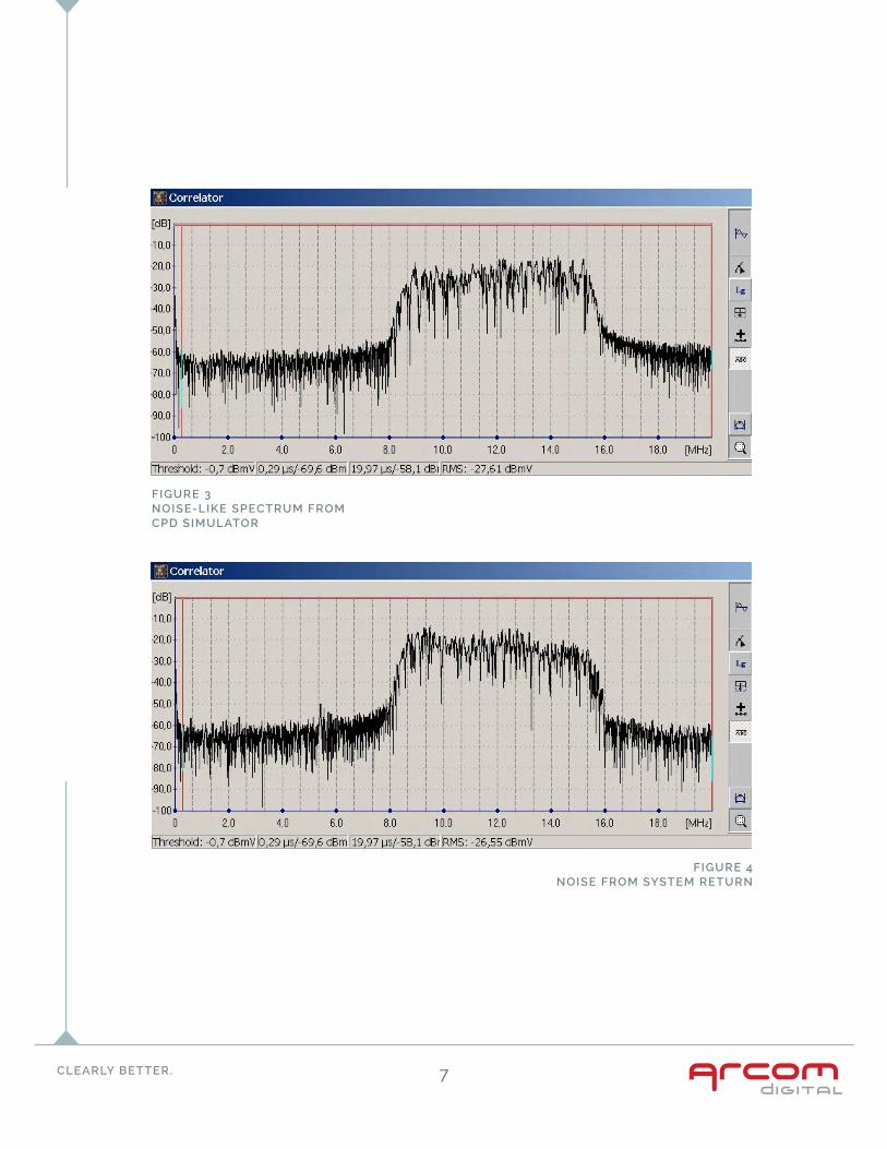
Figures 3 and 4 show the output

signals from the CPD Simulator

and the return path.

NOISE LIKE SIGNAL

Forward signal input

XCOR OUTPUT

CORRELATOR

CPD SIMULATOR

Calculate the Instaneous CPD Signature

RETURN SIGNAL INPUT (NOISE)

Compare each time shifted channel to the return noise signal

To

2 To

3 To

N To

(50 - 1,000 MHz)

SYSTEM ANALOG & DIGITAL CHANNELS

Spike is the time distance to the CPD source

HEADEND COMBINING NETWORK

-100

-90.0

-80.0

-70.0

-60.0

-50.0

-40.0

-30.0

-20.0

-10.0

[dB]

2.00 4.0 6.0 8.0 10.0 12.0 16.014.0 18.0 [MHz]

-100

-90.0

-80.0

-70.0

-60.0

-50.0

-40.0

-30.0

-20.0

-10.0

[dB]

2.00 4.0 6.0 8.0 10.0 12.0 16.014.0 18.0 [MHz]

XC

OR

HU

NT

ER

RA

DA

R

-100

-90.0

-80.0

-70.0

-60.0

-50.0

-40.0

-30.0

-20.0

-10.0

[dB]

2.00 4.0 6.0 8.0 [MHz]

-100

-90.0

-80.0

-70.0

-60.0

-50.0

-40.0

-30.0

-20.0

-10.0

[dB]

2.00 4.0 6.0 8.0 [MHz]

-100

-90.0

-80.0

-70.0

-60.0

-50.0

-40.0

-30.0

-20.0

-10.0

[dB]

2.00 4.0 6.0 8.0 [MHz]

-100

-90.0

-80.0

-70.0

-60.0

-50.0

-40.0

-30.0

-20.0

-10.0

[dB]

2.00 4.0 6.0 8.0 [MHz]

-100

-90.0

-80.0

-70.0

-60.0

-50.0

-40.0

-30.0

-20.0

-10.0

[dB]

2.00 4.0 6.0 8.0 [MHz]

-100

-90.0

-80.0

-70.0

-60.0

-50.0

-40.0

-30.0

-20.0

-10.0

[dB]

2.00 4.0 6.0 8.0 [MHz]

-100

-90.0

-80.0

-70.0

-60.0

-50.0

-40.0

-30.0

-20.0

-10.0

[dB]

2.00 4.0 6.0 8.0 [MHz]

-100

-90.0

-80.0

-70.0

-60.0

-50.0

-40.0

-30.0

-20.0

-10.0

[dB]

2.00 4.0 6.0 8.0 [MHz]

-100

-90.0

-80.0

-70.0

-60.0

-50.0

-40.0

-30.0

-20.0

-10.0

[dB]

2.00 4.0 6.0 8.0 10.0 12.0 16.014.0 18.0 [MHz]

CLEARLY BETTER. 6

FIG

UR

E 2

CLEARLY BETTER. 7

FIGURE 3 NOISE-LIKE SPECTRUM FROM CPD SIMULATOR

FIGURE 4NOISE FROM SYSTEM RETURN

CLEARLY BETTER. 8

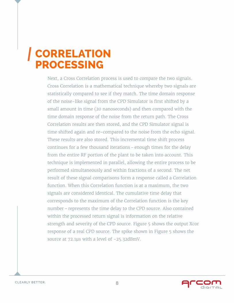
Next, a Cross Correlation process is used to compare the two signals.

Cross Correlation is a mathematical technique whereby two signals are

statistically compared to see if they match. The time domain response

of the noise-like signal from the CPD Simulator is first shifted by a

small amount in time (20 nanoseconds) and then compared with the

time domain response of the noise from the return path. The Cross

Correlation results are then stored, and the CPD Simulator signal is

time shifted again and re-compared to the noise from the echo signal.

These results are also stored. This incremental time shift process

continues for a few thousand iterations – enough times for the delay

from the entire RF portion of the plant to be taken into account. This

technique is implemented in parallel, allowing the entire process to be

performed simultaneously and within fractions of a second. The net

result of these signal comparisons form a response called a Correlation

function. When this Correlation function is at a maximum, the two

signals are considered identical. The cumulative time delay that

corresponds to the maximum of the Correlation function is the key

number – represents the time delay to the CPD source. Also contained

within the processed return signal is information on the relative

strength and severity of the CPD source. Figure 5 shows the output Xcor

response of a real CPD source. The spike shown in Figure 5 shows the

source at 72.1μs with a level of -25.32dBmV.

CORRELATION PROCESSING

CLEARLY BETTER. 9

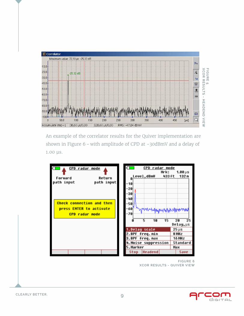
An example of the correlator results for the Quiver implementation are

shown in Figure 6 – with amplitude of CPD at -30dBmV and a delay of

1.00 μs.

FIGURE 6XCOR RESULTS - QUIVER VIEW

FIG

UR

E 5

XC

OR

RE

SU

LT

S - H

EA

DE

ND

VIE

W

CLEARLY BETTER. 10

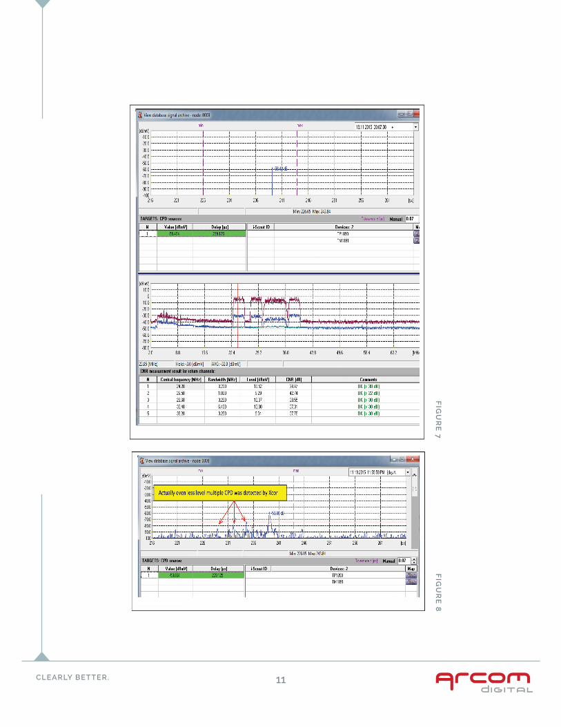
Figures 7 and 8 illustrate an example of how CPD is detected by Xcor

while the RTN spectrum is absolutely clean with the CNR upstream at

a level of >35dB. Following these images, Figures 9 and 10 illustrate

how Hunter records and displays how a small level of CPD may increase

during a short period of time – impacting service at the RTN. The top

part of the screen shows the correlator results and displays CPD events

with a corresponding amplitude and delay. The bottom portion of the

screen shows the return path spectrum and provides a weighted CNR

calculation of all the return carriers, to be used for prioritizing repair.

The first screen capture in Figure 9 shows an example of CPD that is

not yet network affecting. The second screen shot shows the same

source only two hours later, when the CPD level

increased by 26dB to the point that it became

network affecting and deteriorated the return

channel CNR.

These two images provide a great illustration

of the predictive capability of Xcor. With CPD

and the associated corrosion and network

deficiency, the only certainty is that it will

continue to deteriorate itself over time. With

the clear visibility provided by Xcor, you can

fix the impairment before it becomes network

affecting. This ability makes Xcor truly a

game-changer in how the modern network

can be maintained.

PREDICTIVE ELEMENTS

CLEARLY BETTER. 11

FIG

UR

E 7

FIG

UR

E 8

CLEARLY BETTER. 12

FIG

UR

E 9

FIG

UR

E 10

The same CPD two hours later

CLEARLY BETTER. 13

WWW.ARCOMDIGITAL.COM

FOR MORE INFORMATION CALL /800.448.1655

OUTSIDE THE U.S. DIAL / +1 .315.422.1230