WORKSHOP 1 STEADY STATE HEAT TRANSFER WORKSHOP 1 STEADY STATE HEAT TRANSFER.
20
WORKSHOP 1 STEADY STATE HEAT TRANSFER
-
Upload
kenneth-maxwell -
Category
Documents
-
view
231 -
download
0
Transcript of WORKSHOP 1 STEADY STATE HEAT TRANSFER WORKSHOP 1 STEADY STATE HEAT TRANSFER.

WORKSHOP 1
STEADY STATE HEAT TRANSFER
WORKSHOP 1
STEADY STATE HEAT TRANSFER

Mar120, Workshop 10, March 2001 WS 1-2

Mar120, Workshop 10, March 2001 WS 1-3
Model Description
In this Exercise, the following structure will be subjected to the designated thermal (temperature and convective) loading and analyzed to determine the steady-state temperature distribution.

Mar120, Workshop 10, March 2001 WS 1-4
Objective Demonstrate the use of thermal analysis with temperature loading.
Required A file named Thermal_structural.ses in your working directory
(Ask your instructor for it if you don’t see it before starting.)
Mar120, Workshop 10, March 2001 WS 1-5
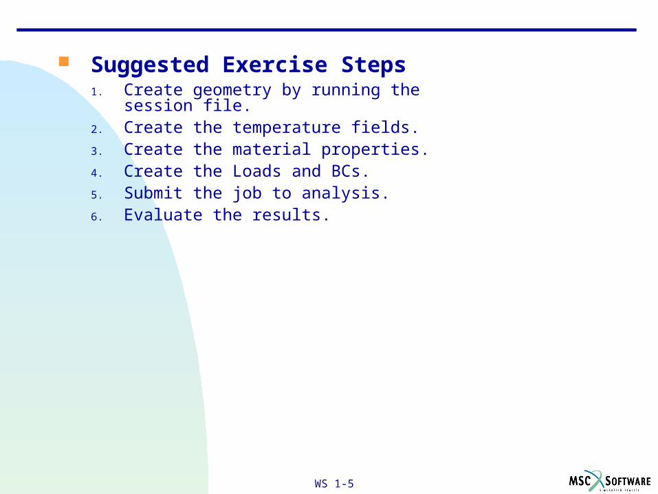
Suggested Exercise Steps1. Create geometry by running the session file.2. Create the temperature fields.3. Create the material properties.4. Create the Loads and BCs.5. Submit the job to analysis.6. Evaluate the results.

Mar120, Workshop 10, March 2001 WS 1-6
CREATE NEW DATABASE
Open a new database. Name it thermal_structural.db
a. File: New
b. Enter thermal_structural.db as the file name.
c. Click OK.d. Enter 2.00 for the Model
Dimension. e. Select MSC.Marc as the
Analysis Code. f. Select Thermal as the
Analysis Type.g. Click OK.
a
thermal_structural b
MSC.Marc e
Thermal f
g
2.00 d
c

Mar120, Workshop 10, March 2001 WS 1-7
Step 1. Run the Provided Session File
Create necessary geometry by playing the session file.
a. File: Session / Play.
b. Select Thermal_structural.ses.
c. Click Apply.
Thermal_structural
Thermal_structural.sesc
b
After clicking Apply, you will see the model being constructed automatically by the session file.
Your model should look like this.
a

Mar120, Workshop 10, March 2001 WS 1-8
Step 2. Fields: Create / Material Property / Tabular Input
Define temperature dependent material property table for conductivity.
a. Fields: Create / Material Property / Tabular Input.
b. Enter conductivity field for Field Name.
c. Select Temperature (T) for Active Independent Variables.
d. Click Input Data…Enter the following values:
e. Click OK.
f. Click Apply.
T Value100 14.6538600 22.6087
1400 31.8197 e
conductivity field
a
b
f
c
d
To modify the content of a particular cell, first click on that cell, then type number in Input Scalar Data box and press Enter.
Mar120, Workshop 10, March 2001 WS 1-9
Conductivity_fieldd
e
f
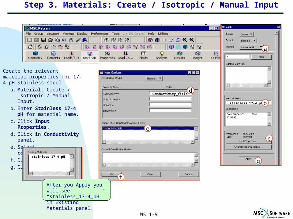
Step 3. Materials: Create / Isotropic / Manual Input
Create the relevant material properties for 17-4 pH stainless steel
a. Material: Create / Isotropic / Manual Input.
b. Enter Stainless 17-4 pH for material name.
c. Click Input Properties.
d. Click in Conductivity panel.
e. Select conductivity_field.
f. Click OK.
g. Click Apply.
stainless 17-4 pH
After you Apply you will see “stainless_17-4_pH” in Existing Materials panel.
stainless 17-4 pH
a
b
c
g

Mar120, Workshop 10, March 2001 WS 1-10
Step 4. Properties: Create / 3D / Solid
Apply the steel properties to the model
a. Properties: Create / 3D / Solid.
b. Enter Prop thermal for Property Set Name.
c. Click Input Properties.
d. Click in Material Name panel.
e. Select Stainless_17-4_PH.
f. Click OK.
g. Click in the Select Members panel.
Stainless 17-4 pH d
e
f
Prop thermal
a
b
c
g
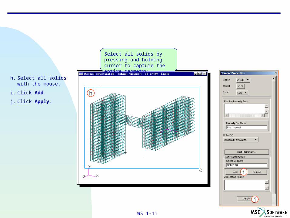
Mar120, Workshop 10, March 2001 WS 1-11
h. Select all solids with the mouse.
i. Click Add.
j. Click Apply.
h
Select all solids by pressing and holding cursor to capture the entire geometry
i
j

Mar120, Workshop 10, March 2001 WS 1-12
Create the temperature loading at the fixed end faces.
a. Loads/BCs: Create / Temp (thermal) / Nodal.
b. Enter left_edge for New Set Name.
c. Click Input Data.
d. Enter 50 for Temperature.
e. Click OK.
f. Click Select Application Region.
g. Click in Select Geometry Entities panel.
h. Select Surface or Face picking icon.
Step 5. Loads/BCs: Create / Temp (Thermal) / Nodal
left_edge
a
b
c
f
50 d
e
g
h
Mar120, Workshop 10, March 2001 WS 1-13
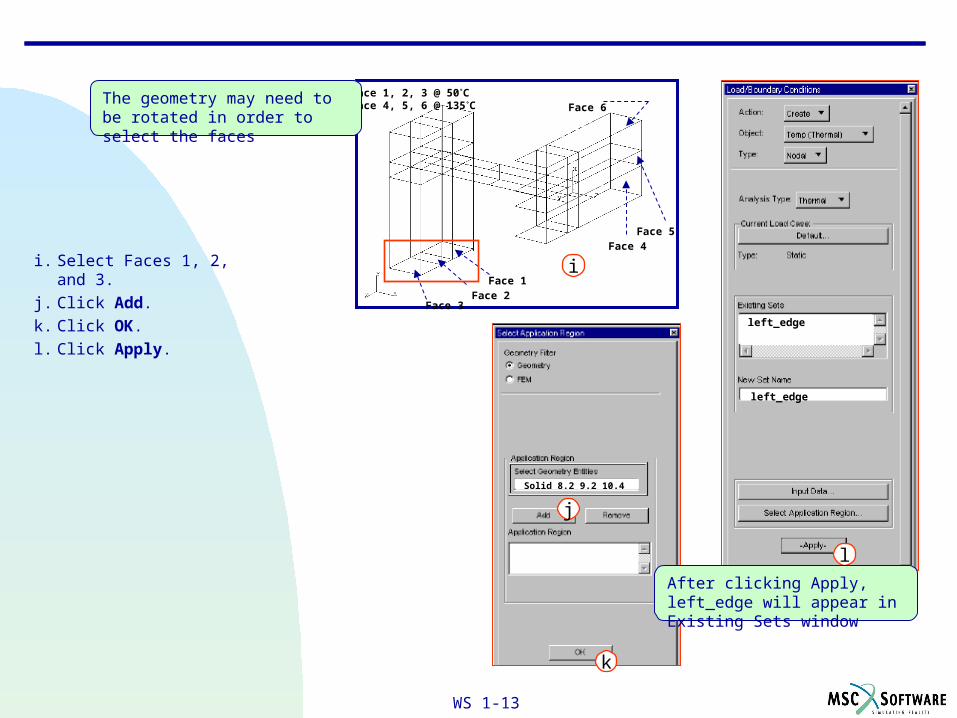
i. Select Faces 1, 2, and 3.
j. Click Add.
k. Click OK.
l. Click Apply.
left_edge
left_edge
l
Solid 8.2 9.2 10.4
j
k
Face 1, 2, 3 @ 50°CFace 4, 5, 6 @ 135°C
Face 3Face 2
Face 1
Face 4Face 5
Face 6
i
The geometry may need to be rotated in order to select the faces
After clicking Apply, left_edge will appear in Existing Sets window
Mar120, Workshop 10, March 2001 WS 1-14
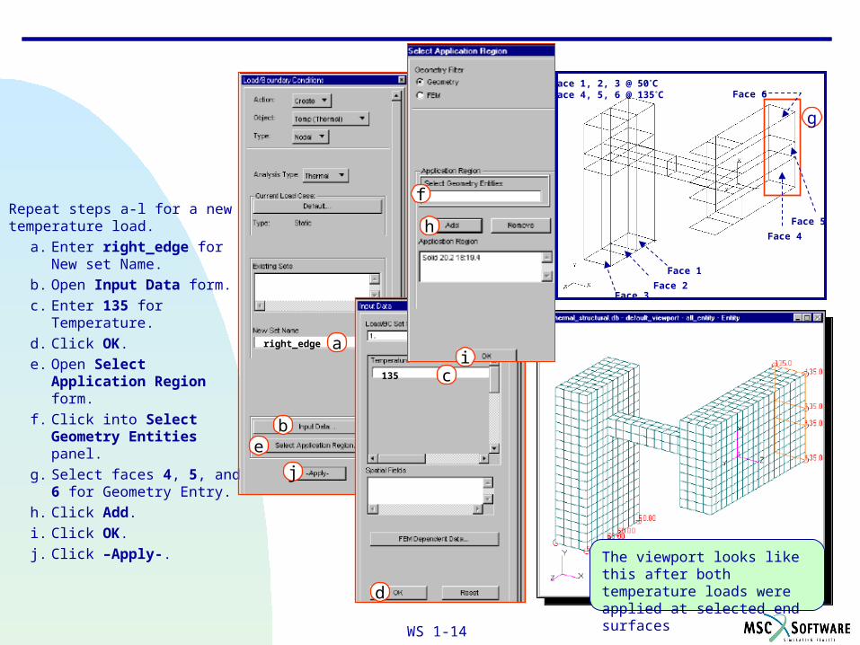
Repeat steps a-l for a new temperature load.
a. Enter right_edge for New set Name.
b. Open Input Data form.
c. Enter 135 for Temperature.
d. Click OK.
e. Open Select Application Region form.
f. Click into Select Geometry Entities panel.
g. Select faces 4, 5, and 6 for Geometry Entry.
h. Click Add.
i. Click OK.
j. Click –Apply-.
Face 1, 2, 3 @ 50°CFace 4, 5, 6 @ 135°C
Face 3Face 2
Face 1
Face 4
Face 5
Face 6
g
The viewport looks like this after both temperature loads were applied at selected end surfaces
right_edge a
be
j
135 c
d
f
i
h
Mar120, Workshop 10, March 2001 WS 1-15
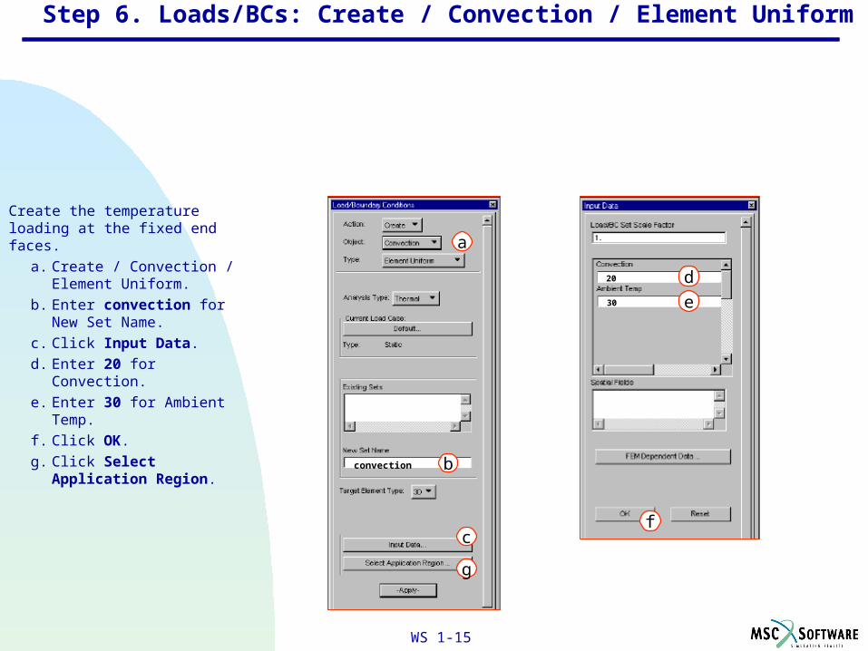
Step 6. Loads/BCs: Create / Convection / Element Uniform
Create the temperature loading at the fixed end faces.
a. Create / Convection / Element Uniform.
b. Enter convection for New Set Name.
c. Click Input Data.
d. Enter 20 for Convection.
e. Enter 30 for Ambient Temp.
f. Click OK.
g. Click Select Application Region.
30
20 d
e
f
convection
a
b
c
g

Mar120, Workshop 10, March 2001 WS 1-16
h. Click in Select Solids Faces panel.
i. Select Free face of solid picking icon.
j. Select the four outer middle bar surfaces by partly enclosing them with view corner picking.
k. Click Add.
l. Click OK.
m. Click -Apply-.
m
j
This picks the four larger surfaces bounding the central body when you use the default picking options.
Solid 1:11:10.1 1:11:10.2 1:11:10.3 1:11:10.4
hk
l
After clicking Add, the selected solid will appear in the Application Region window as shown
i

Mar120, Workshop 10, March 2001 WS 1-17
Step 7. Analysis: Analyze / Entire Model / Full Run
Submit the model for thermal analysis.
a. Analysis: Analyze / Entire Model / Full Run.
b. Enter thermal_job1 for Job Name.
c. Click Load Step Creation.
d. Enter thermal for Job Step Name.
e. Click Apply.
f. Click Cancel.
thermal_job1
a
b
c
thermal d
e f
After clicking apply, thermal will appear in the Available Job Steps window along with the “Default Static: Step”

Mar120, Workshop 10, March 2001 WS 1-18
g. Click Load Step Selection.
h. Select thermal in Existing Job Steps window.
i. Deselect Default Static Step.
j. Click OK.
k. Click Apply.
g
k
Make sure thermal is the only entry in the Selected Job Steps window. If Default Static Step shows up, remove it by clicking on it.
Once the Analysis is launched, you can monitor the progress of the job by looking at the thermal_job1.out and thermal_job1.sts files.
h
j
i
Mar120, Workshop 10, March 2001 WS 1-19
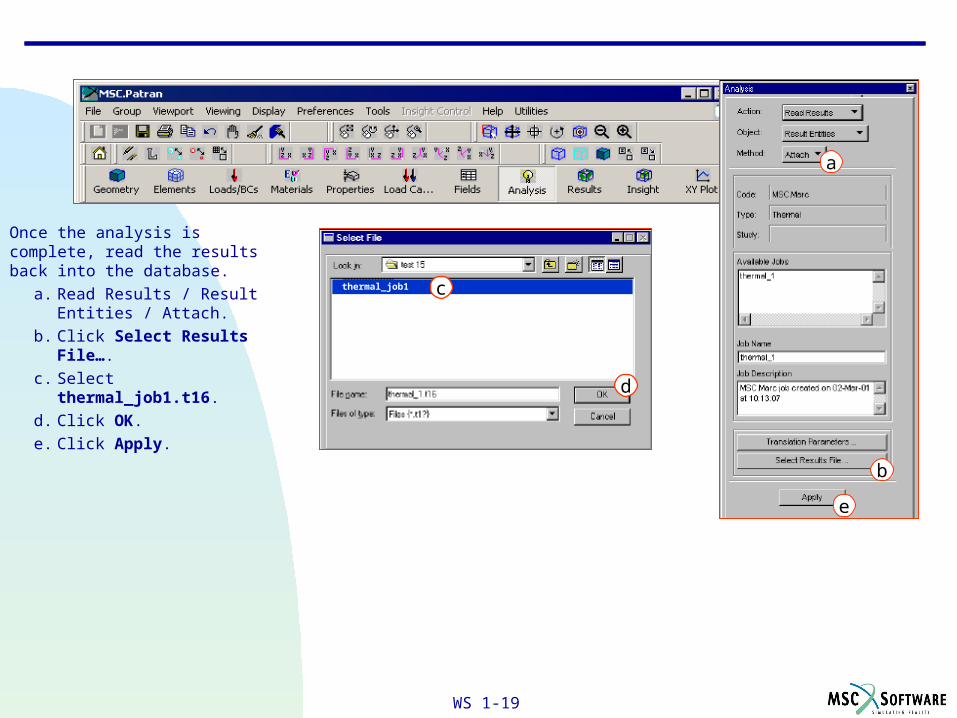
Once the analysis is complete, read the results back into the database.
a. Read Results / Result Entities / Attach.
b. Click Select Results File….
c. Select thermal_job1.t16.
d. Click OK.
e. Click Apply.
thermal_job1 c
d
a
b
e

Mar120, Workshop 10, March 2001 WS 1-20
Step 8. Results: Create / Quick Plot
Post process the results of the thermal analysis.
a. Results: Create / Quick plot.
b. Click Reset Graphics.
c. Select Temperature, Nodal in Select Fringe Result window.
d. Click Apply.
The steady state temperature distribution should look like this in the viewport window.
ba
c
d